Revealing the Ionization Properties of the Magellanic Stream using Optical Emission

Abstract

The Magellanic Stream, a gaseous tail that trails behind the Magellanic Clouds, could replenish the Milky Way with a tremendous amount of gas if it reaches the Galactic disk before it evaporates into the halo. To determine how the Magellanic Stream’s properties change along its length, we have conducted an observational study of the H$\alpha$ emission, along with other optical warm ionized gas tracers, toward $39$ sight lines. Using the Wisconsin H$\alpha$ Mapper telescope, we detect H$\alpha$ emission brighter than $30-50~{}{\rm mR}$ in $26$ of our $39$ sight lines. This H$\alpha$ emission extends more than $2\arcdeg$ away from the H i emission. By comparing $I_{\rm H\alpha}$ and $I_{\rm[O\textsc{~{}i}]}$, we find that regions with $\log N_{\rm H\textsc{~{}i}}/\,\mathrm{cm}^{-2}\approx 19.5-20.0$ are $16-67\%$ ionized. Most of the $I_{\rm H\alpha}$ along the Magellanic Stream are much higher than expected if the primary ionization source is photoionization from Magellanic Clouds, the Milky Way, and the extragalactic background. We find that the additional contribution from self ionization through a “shock cascade” that results as the Stream plows through the halo might be sufficient to reproduce the underlying level of H$\alpha$ emission along the Stream. In the sparsely sampled region below the South Galactic Pole, there exists a subset of sight lines with uncharacteristically bright emission, which suggest that gas is being ionized further by an additional source that could be a linked to energetic processes associated with the Galactic center.

1 Introduction

Star formation in galaxies is regulated by their ability to accrete and retain gas. Chemical evolution models require the inflow of low-metallicity gas to explain the observed stellar abundance patterns of the Milky Way (MW; e.g., Chiappini 2008). The star-formation rates of $L^{*}$ galaxies indicates that they will quickly exhaust their gas reservoirs making stars without external sources of gas that they accrete onto their disks (Erb 2008; Hopkins et al. 2008; Putman et al. 2012; Sánchez Almeida et al. 2014). Our own galaxy will deplete its gas supplies in only $1-2~{}{\rm Gyrs}$ at its present star-formation rate (Larson et al. 1980) of $1-3~{}{\rm M}_{\odot}~{}\,\mathrm{yr}^{-1}$ (e.g., Robitaille & Whitney 2010; Chomiuk & Povich 2011). With the MW’s long history of consistently forming stars (e.g., Rocha-Pinto et al. 2000), this rapid gas depletion time suggests that our galaxy has sustained itself by acquiring gas from external sources. These sources include primordial material that is left over from the formation of the universe and material that is ripped from nearby dwarf galaxies, such as the tidal remnants of the Magellanic Clouds (MCs). However, the recent results of Mutch et al. (2011) show that the MW’s star-formation rate could be in decline and that the Galaxy is likely in the process of transitioning from the “green valley” to the “red sequence”. Although numerous clouds surround the MW as detected in neutral (e.g., Kalberla et al. 2005, Wakker et al. 2007, 2008 and Saul et al. 2012) and ionized gas (e.g., Sembach et al. 2003, Fox et al. 2006, Hill et al. 2009, Lehner & Howk 2011, Barger et al. 2012, and Lehner et al. 2012), it is unclear how much of that gas will reach the Galactic disk to provide replenishment. Interactions with high-temperature coronal gas in the halo combined with an ionizing radiation field from a number of sources may heat and ionize inflowing gas, hindering accretion (see Putman et al. 2012 for review).

However, the MW’s gas crisis might soon be over as it has recently captured the gas-rich MCs (e.g., Besla et al. 2007), which may provide enough gas to sustain or even boost its star formation (FWB14: Fox et al. 2014). Galaxy interactions have stripped more than $2\times 10^{9}~{}{\rm M}_{\odot}$ of neutral and ionized gas from the Large and Small Magellanic Clouds (SMC & LMC; e.g., Brüns et al. 2005; Bland-Hawthorn et al. 2007; Barger et al. 2013; Fox et al. 2005, 2014). This debris spans over $200\arcdeg$ on the sky (Nidever et al. 2010) and is especially concentrated at $b<0\arcdeg$ (Putman et al. 1998). The tidal structures known as the Magellanic Stream and Leading Arm could supply the MW with $\sim 3-7~{}{M_{\odot}}~{}{\rm yr}^{-1}$ (FWB14). However, the exact amount of gas contained within these streams is uncertain due to weak constraints on their distance. Additionally, much of this material will likely evaporate into the Galactic halo before reaching the star-forming disk. Although the evaporated gas will build the halo, it could eventually condense, fall to the disk, and replenish the Milky Way’s star-formation gas reservoir on longer timescales (e.g., Joung et al. 2012).

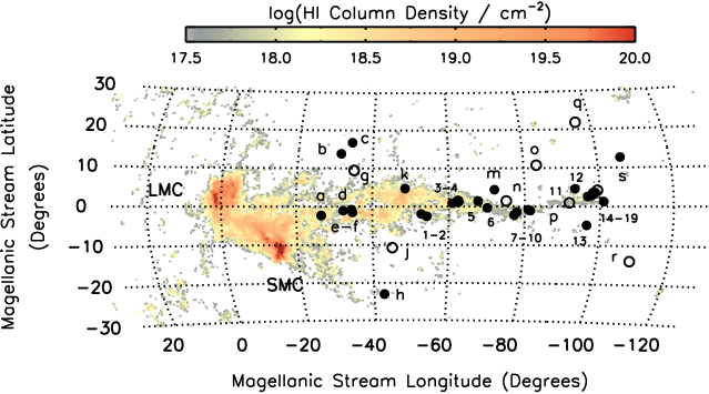
Figure 1: Locations of pointed WHAM observations along the Magellanic Stream, where the letters and numbers coincide with the sight line identifiers listed in Table 1. Filled and open circles denote H$\alpha$ detections and non-detections, respectively. The background H i column density gas map of the Magellanic System is comprised of the Gaussian decompositions of the Leiden-Argentine-Bonn (LAB) all-sky survey adapted from Nidever et al. (2008).

The trailing tidal debris, known as the Magellanic Stream, contains $\gtrsim 10^{8}~{}{M_{\odot}}$ in H i gas alone (Brüns et al. 2005) and over three times that in ionized gas (FWB14). Its elongated structure substantially increases its surface area, which increases its exposure to the surrounding coronal gas and ionizing radiation field. Further, numerous cloudlets may have splintered off of or evaporated away from the two main filaments of the Stream (Putman et al. 2003b; For et al. 2014; see Figure 1), making them even more susceptible to their environment. Bland-Hawthorn et al. (2007) and Heitsch & Putman (2009) found that clouds with H i masses of less than $10^{4.5}~{}{\rm M}_{\odot}$ may become fully ionized through Kelvin-Helmholtz instabilities within $\sim 100~{}{\rm Myr}$ due to interactions with surrounding coronal gas. Although the Stream is quite massive in its entirety, the morphology of the neutral gas is fragmented and the numerous, small offset clouds (Westmeier & Koribalski 2008 and Stanimirović et al. 2008) suggest that it is evaporating. Nigra et al. (2012) examined the H i morphology of one of the small clouds that fragmented off of the Magellanic Stream and found that it has a cold and dense core that is enclosed within a warm extended envelope. They illustrate that its diffuse skin was likely a result of turbulence that was generated by the cloud rubbing against the surrounding coronal gas and not by conductive heating. Additionally, clouds are eroded away by the ionizing radiation field of the MW, nearby galaxies, and extragalactic background (EGB). Determining the properties of both the neutral and ionized gas phases is vital for ascertaining how the Magellanic Stream is affected by its environment.

The strength of the incident ionizing radiation field and of the ram-pressure stripping effects from the surrounding coronal gas on the Magellanic Stream strongly depend on its position relative to nearby galaxies and its location within the Galactic halo. Its distance is only known where the Magellanic Stream originates at the MCs. Observationally, Lehner et al. (2012) found that the trailing end of the Stream must lie further than $20~{}\,\mathrm{kpc}$ away due to the lack of absorption seen toward stellar targets and from the abundance of absorption detected toward active galactic nuclei (AGN) in the same vicinity (Lehner & Howk 2011). Because the MCs are just past perigalacticon in their orbits (see D’Onghia & Fox 2016 for a review) and because the Magellanic Stream is a trailing Stream, the closest possible distance to the trailing gas is the present distances of the MCs (i.e., $d\gtrsim 50~{}\,\mathrm{kpc}$). Galaxy interaction models of this system predict that the trailing gas in the Stream could lie as far as $100-200~{}\,\mathrm{kpc}$ from the Galactic center (e.g., Besla et al. 2010, 2012, Diaz & Bekki 2011, 2012, and Guglielmo et al. 2014). The most recent models predict that these galaxies are on a highly elliptical orbit when accounting for (i) an increase in the measured proper motions from Hubble Space Telescope observations of the LMC and SMC by a third (Kallivayalil et al. 2006) and (ii) decreases in the total mass estimates of the Galactic halo (e.g., Kafle et al. 2012; McMillan 2017). More work is still needed to produce a physically consistent Stream as only the Guglielmo et al. (2014) simulation includes both the neutral and ionized gas contained within the Stream, the existing models exclude either the effect of ram-pressure stripping or photoionization, and only Besla et al. (2010, 2012) includes cooling (radiative only). However, it is also important to note that the further the Magellanic Stream lies from the MW, the less it will be influenced by ram-pressure stripping from the MW’s coronal halo gas and its ionizing radiation field.

Numerous studies have detected ionized gas in the Magellanic Stream along individual lines of sight, including through H$\alpha$ emission (WW96: Weiner & Williams 1996; WVW02; WVW02: Weiner et al. 2002, W03: W03: Weiner 2003, PBV03: Putman et al. 2003a, YKY12: Yagi et al. 2012, and BMS13: Bland-Hawthorn et al. 2013) and UV absorption (e.g., Sembach et al. 2003 , Lehner et al. 2012, Richter et al. 2013, and Fox et al. 2005, 2010, 2014). Because some of these H$\alpha$ detections are brighter than expected if the primary source of their ionization is the MW’s ionizing radiation field and the EGB, other ionization sources are also thought to contribute. However, previous studies have neglected the ionizing contribution from the MCs themselves, which we account for in this study.

We describe our multiline observations of the warm ionized gas emission of the Magellanic Stream in Section 2 and their reduction in Section 3. We compare the neutral gas as traced by H i emission with the ionized gas in Section 4 by examining their kinematics, emission strengths, distribution, and ionization fraction. We then discuss how well the observed H$\alpha$ emission of the Stream can be reproduced by photoionization alone from the surrounding galaxies (MW, LMC, and SMC) and the EGB, photoionization plus collisional ionization from interactions with the Galactic halo and with the Stream itself, and energetic processes that are associated with the Galactic center in Section 5. We finally summarize our major conclusions in Section 6.

2 Observations

Our $39$ pointed observations of the warm ionized gas ($\sim 10^{4}~{}{\rm K}$) in the Magellanic Stream span over $100\arcdeg$ along its length. To assess the extent of the ionized gas, many of these observations lie off the H i emission ($\log{N_{\rm H\textsc{~{}i}}/\,\mathrm{cm}^{-2}}\lesssim 18$), as illustrated in Figure 1. We preferentially aligned the observations at positions (a–s; see Figure 1 and Table 1) toward bright background quasars with existing absorption-line observations. In the complementary FWB14 study, we combined the aligned emission- and absorption-line observations to further explore how ionization conditions of the Stream vary along its length. We aligned the observations at positions (1–19; see Figure 1 and Table 1) with the main H i filamentary structures of the Magellanic Stream.

Table 1: WHAM Spectroscopic Observations

			On Target				Off Target				Notes
ID	Filter	${\rm v}_{\rm{LSR}}$	$l_{\rm MS},~{}b_{\rm MS}$	$l,~{}b$	Exposure Time		$l_{\rm MS},~{}b_{\rm MS}$	$l,~{}b$	Exposure Time
		(${\rm km\thinspace s^{-1}}$)	(degrees)	(degrees)	(s)		(degrees)	(degress)	(s)
a	H$\alpha$	$+80,+280$	$-26.6$, $-02.3$	$295.1$, $-57.8$	$10\times 60$		$-24.2$, $\phantom{-}00.8$	$288.5$, $-56.4$	$12\times 60$		FAIRALL 9
b	H$\alpha$	$+45,+245$	$-31.5$, $\phantom{-}13.8$	$262.3$, $-63.9$	$18\times 60$		$-33.8$, $\phantom{-}16.7$	$256.8$, $-02.5$	$18\times 60$		Near HE0226-4110
c	H$\alpha$	$+45,+245$	$-34.3$, $\phantom{-}16.8$	$253.9$, $-65.8$	$15\times 60$		$-32.7$, $-08.6$	$311.3$, $-60.7$	$18\times 60$		HE0226-4110
d	H$\alpha$	$+5,+205$	$-32.3$, $-01.0$	$296.4$, $-63.7$	$15\times 60$		$-32.7$, $-08.6$	$311.3$, $-60.7$	$18\times 60$		Near RBS 144
e	H$\alpha$	$+5,+205$	$-34.8$, $-01.5$	$299.5$, $-65.8$	$15\times 60$		$-32.7$, $-08.6$	$311.3$, $-60.7$	$18\times 60$		RBS 144
f	H$\alpha$	$+5,+205$	$-34.5$, $-00.8$	$297.5$, $-65.8$	$16\times 60$		$-35.1$, $-02.3$	$301.5$, $-65.8$	$16\times 60$		Near RBS 144
g	H$\alpha$	$+150,+350$	$-35.1$, $\phantom{-}09.5$	$271.8$, $-68.9$	$12\times 60$		$-32.8$, $\phantom{-}13.9$	$261.4$, $-65.1$	$14\times 60$		HE0153-4520
h	H$\alpha$	$+55,+255$	$-42.8$, $-23.0$	$343.9$, $-56.4$	$16\times 60$		$-46.6$, $-20.2$	$347.9$, $-60.4$	$15\times 60$		Near RBS 1892
j	H$\alpha$	$+100,+300$	$-45.2$, $-10.7$	$334.9$, $-68.2$	$15\times 30$		$-45.7$, $-08.7$	$332.9$, $-70.2$	$16\times 30$		ES0292-G24
k	H$\alpha$	$+45,+245$	$-48.6$, $\phantom{-}04.7$	$295.7$, $-80.9$	$16\times 30$		$-48.5$, $\phantom{-}05.0$	$293.7$, $-80.9$	$15\times 30$		Near HE0056-3622
m	H$\alpha$	$-245,-45$	$-72.0$, $\phantom{-}04.4$	$87.5$, $-75.0$	$12\times 60$		$119.9$, $-05.3$	$93.6$, $-72.4$	$12\times 60$		Near PHL2525
n	H$\alpha$	$-245,-45$	$-75.1$, $\phantom{-}01.5$	$80.7$, $-71.2$	$10\times 60$		$119.9$, $-05.3$	$93.6$, $-72.4$	$12\times 60$		PHL2525
o	H$\alpha$	$-245,-45$	$-83.4$, $\phantom{-}10.8$	$107.7$, $-64.0$	$13\times 60$		$-80.9$, $\phantom{-}09.1$	$104.1$, $-66.6$	$14\times 60$		UM239
p	H$\alpha$	$-315,-115$	$-90.8$, $-00.7$	$86.2$, $-55.6$	$17\times 60$		$-91.3$, $\phantom{-}01.5$	$90.2$, $-55.6$	$17\times 60$		Near NGC7714
q	H$\alpha$	$-295,-95$	$-95.9$, $\phantom{-}21.8$	$123.8$, $-50.2$	$15\times 60$		$-99.8$, $\phantom{-}19.3$	$118.8$, $-47.1$	$15\times 60$		MRK 1502
r	H$\alpha$	$-295,-95$	$-109.2$, $-13.9$	$76.0$, $-34.2$	$15\times 60$		$-109.7$, $-12.3$	$77.8$, $-34.2$	$16\times 60$		MRK 304
s	H$\alpha$	$-430,-230$	$-106.4$, $\phantom{-}12.6$	$108.8$, $-41.4$	$15\times 60$		$-104.9$, $\phantom{-}09.2$	$104.1$, $-42.9$	$16\times 60$		MRK 335
1	H$\alpha$	$-184,+14$	$-52.8$, $-01.9$	$342.6,-79.6$	$19\times 120$		$-54.6$, $-06.4$	$357.4$, $-75.8$	$20\times 120$		BMS13
2	H$\alpha$	$-184,+14$	$-54.3$, $-02.5$	$351.7,-79.5$	$7\times 120$		$-55.8$, $-07.2$	$2.7$, $-75.2$	$7\times 120$		BMS13
3	H$\alpha$	$-203,-3$	$-60.9$, $\phantom{-}00.9$	$37.5,-82.5$	$4\times 300$		$-63.5$, $-03.9$	$37.0$, $-77.0$	$5\times 300$		BMS13
4a	H$\alpha$	$-221,-21$	$-62.4$, $\phantom{-}01.4$	$48.6,-82.0$	$2\times 300$		$-63.1$, $\phantom{-}12.9$	$142.4$, $-82.2$	$3\times 300$		BMS13
4b	H$\alpha$	$-201,-1$	$-62.5$, $\phantom{-}01.4$	$49.0,-82.0$	$3\times 300$		$-67.9$, $\phantom{-}04.3$	$82.0$, $-79.0$	$1\times 300$		BMS13
5a	H$\alpha$	$-200,0$	$-67.7$, $\phantom{-}01.5$	$68.9,-78.0$	$3\times 300$		$-67.9$, $\phantom{-}04.3$	$82.0$, $-79.0$	$6\times 300$		BMS13
5b	H$\alpha$	$-220,-20$	$-67.7$, $\phantom{-}01.4$	$68.7,-78.0$	$2\times 300$		$-63.1$, $\phantom{-}12.9$	$142.4$, $-82.2$	$3\times 300$		BMS13
6	H$\alpha$	$-202,-2$	$-70.1$, $-00.3$	$67.5,-75.0$	$6\times 300$		$-70.6$, $-04.0$	$58.0$, $-72.5$	$6\times 300$		BMS13
7a	H$\alpha$	$-373,-173$	$-77.2$, $-02.1$	$73.5,-68.0$	$4\times 300$		$-77.0$, $-05.3$	$66.0$, $-66.5$	$4\times 300$		BMS13
7b	H$\alpha$	$-305,-105$	$-77.2$, $-02.2$	$73.3,-67.9$	$7\times 120$		$-81.0$, $-03.4$	$74.5$, $-64.0$	$13\times 120$		BMS13
8	H$\alpha$	$-306,-106$	$-77.9$, $-01.4$	$75.8,-67.6$	$7\times 120$		$-81.0$, $-03.4$	$74.5$, $-64.0$	$13\times 120$		BMS13
9	H$\alpha$	$-372,-172$	$-80.9$, $-00.8$	$80.0,-65.0$	$3\times 300$		$-67.9$, $\phantom{-}04.3$	$82.0$, $-79.0$	$3\times 300$		BMS13
10	H$\alpha$	$-373,-172$	$-81.4$, $-01.0$	$80.0,-64.5$	$4\times 300$		$-80.2$, $\phantom{-}01.8$	$85.5$, $-66.5$	$4\times 300$		BMS13
11	H$\alpha$	$-441,-241$	$-91.8$, $\phantom{-}01.0$	$89.5,-55.0$	$10\times 300$		$-91.4$, $-02.7$	$83.0$, $-54.5$	$7\times 300$		BMS13
12	H$\alpha$	$-440,-240$	$-93.4$, $\phantom{-}04.6$	$96.0,-54.0$	$10\times 300$		$-91.0$, $\phantom{-}06.2$	$98.5$, $-56.5$	$10\times 300$		BMS13
13	H$\alpha$	$-441,-241$	$-96.5$, $-04.8$	$82.3,-49.0$	$9\times 300$		$-91.4$, $-02.7$	$83.0$, $-54.5$	$7\times 300$		BMS13
14	H$\alpha$	$-439,-239$	$-96.7$, $\phantom{-}02.6$	$93.5,-50.5$	$8\times 300$		$-100.9$, $\phantom{-}04.1$	$96.5$, $-46.5$	$8\times 300$		BMS13
15	H$\alpha$	$-482,-282$	$-97.7$, $\phantom{-}02.8$	$94.0,-49.5$	$4\times 300$		$-100.7$, $\phantom{-}12.0$	$108.0$, $-47.0$	$8\times 300$		BMS13
16	H$\alpha$	$-482,-282$	$-98.3$, $\phantom{-}03.4$	$95.0,-49.0$	$4\times 300$		$-100.7$, $\phantom{-}12.0$	$108.0$, $-47.0$	$16\times 300$		BMS13
17	H$\alpha$	$-481,-281$	$-98.8$, $\phantom{-}03.6$	$95.5,-48.5$	$4\times 300$		$-100.7$, $\phantom{-}12.0$	$108.0$, $-47.0$	$16\times 300$		BMS13
18	H$\alpha$	$-481,-281$	$-99.4$, $\phantom{-}04.2$	$96.5,-48.0$	$4\times 300$		$-100.7$, $\phantom{-}12.0$	$108.0$, $-47.0$	$16\times 300$		BMS13
19	H$\alpha$	$-438,-238$	$-101.0$, $\phantom{-}01.3$	$92.5,-46.0$	$8\times 300$		$-100.9$, $\phantom{-}04.1$	$96.5$, $-46.5$	$8\times 300$		BMS13
a	H$\beta$	$+80,+280$	$-26.6$, $-02.3$	$295.1$, $-57.8$	$10\times 60$		$-24.3$, $\phantom{-}04.3$	$282.2$, $-57.1$	$11\times 60$		FAIRALL 9
e	H$\beta$	$+5,+205$	$-34.8$, $-01.5$	$299.5$, $-65.8$	$23\times 60$		$-32.7$, $-08.6$	$311.3$, $-60.7$	$23\times 60$		RBS 144
a	[S ii]$~{}\lambda 6716$	$+80,+280$	$-26.6$, $-02.3$	$295.1$, $-57.8$	$15\times 60$		$-26.2$, $-01.3$	$293.1$, $-57.8$	$16\times 60$		FAIRALL 9
e	[S ii]$~{}\lambda 6716$	$+5,+205$	$-34.8$, $-01.5$	$299.5$, $-65.8$	$5\times 60$		$-32.7$, $-08.6$	$311.3$, $-60.7$	$6\times 60$		RBS 144
1	[S ii]$~{}\lambda 6716$	$-184,+14$	$-52.8$, $-01.9$	$342.6,-79.6$	$14\times 120$		$-54.6$, $-06.4$	$357.4$, $-75.8$	$14\times 120$		BMS13
2	[S ii]$~{}\lambda 6716$	$-184,+14$	$-54.3$, $-02.5$	$351.7,-79.5$	$11\times 120$		$-55.8$, $-07.2$	$2.7$, $-75.2$	$4\times 120$		BMS13
3	[S ii]$~{}\lambda 6716$	$-175,+25$	$-60.9$, $\phantom{-}00.9$	$37.5,-82.5$	$6\times 300$		$-63.5$, $-03.9$	$37.0$, $-77.0$	$6\times 300$		BMS13
a	[N ii]$~{}\lambda 6583$	$+80,+280$	$-26.6$, $-02.3$	$295.1$, $-57.8$	$15\times 60$		$-26.2$, $-01.3$	$293.1$, $-57.8$	$16\times 60$		FAIRALL 9
e	[N ii]$~{}\lambda 6583$	$+5,+205$	$-34.8$, $-01.5$	$299.5$, $-65.8$	$15\times 60$		$-32.7$, $-08.6$	$311.3$, $-60.7$	$18\times 60$		RBS 144
1	[N ii]$~{}\lambda 6583$	$-184$ to $+14$	$-52.8$, $-01.9$	$342.6,-79.6$	$14\times 120$		$-54.6$, $-06.4$	$357.3$, $-75.8$	$14\times 120$		BMS13
2	[N ii]$~{}\lambda 6583$	$-184,+14$	$-54.3$, $-02.5$	$351.7,-79.5$	$5\times 120$		$-55.8$, $-07.2$	$2.7$, $-75.2$	$5\times 120$		BMS13
3	[N ii]$~{}\lambda 6583$	$-175,+25$	$-60.9$, $\phantom{-}00.9$	$37.5,-82.5$	$8\times 300$		$-63.5$, $-03.9$	$37.0$, $-77.0$	$8\times 300$		BMS13
a	[N ii]$~{}\lambda 5755$	$+80,+280$	$-26.6$, $-02.3$	$295.1$, $-57.8$	$11\times 60$		$-25.0$, $\phantom{-}00.6$	$289.2$, $-57.1$	$12\times 60$		FAIRALL 9
e	[N ii]$~{}\lambda 5755$	$+5,+205$	$-34.8$, $-01.5$	$299.5$, $-65.8$	$15\times 60$		$-32.7$, $-08.6$	$311.3$, $-60.7$	$16\times 60$		RBS 144
a	[O i]$~{}\lambda 6300$	$+80,+280$	$-26.6$, $-02.3$	$295.1$, $-57.8$	$11\times 60$		$-25.0$, $\phantom{-}00.6$	$289.2$, $-57.1$	$12\times 60$		FAIRALL 9
e	[O i]$~{}\lambda 6300$	$+5,+205$	$-34.8$, $-01.5$	$299.5$, $-65.8$	$14\times 60$		$-32.7$, $-08.6$	$311.3$, $-60.7$	$16\times 60$		RBS 144
1	[O i]$~{}\lambda 6300$	$-184$ to $+14$	$-52.8$, $-01.9$	$342.6,-79.6$	$25\times 120$		$-54.6$, $-06.4$	$357.4$, $-75.8$	$25\times 120$		BMS13
a	[O ii]$~{}\lambda 7320$	$+80,+280$	$-26.6$, $-02.3$	$295.1$, $-57.8$	$11\times 60$		$-25.0$, $\phantom{-}00.6$	$289.2$, $-57.1$	$12\times 60$		FAIRALL 9
e	[O ii]$~{}\lambda 7320$	$+5,+205$	$-34.8$, $-01.5$	$299.5$, $-65.8$	$15\times 60$		$-32.7$, $-08.6$	$311.3$, $-60.7$	$16\times 60$		RBS 144
1	[O ii]$~{}\lambda 7320$	$-184$ to $+14$	$-52.8$, $-01.9$	$342.6,-79.6$	$12\times 120$		$-54.6$, $-06.4$	$357.4$, $-75.8$	$12\times 120$		BMS13
a	[O iii]$~{}\lambda 5007$	$+5,+205$	$-26.6$, $-02.3$	$295.1$, $-57.8$	$11\times 60$		$-25.0$, $\phantom{-}00.6$	$289.2$, $-57.1$	$12\times 60$		FAIRALL 9
e	[O iii]$~{}\lambda 5007$	$+5,+205$	$-34.8$, $-01.5$	$299.5$, $-65.8$	$15\times 60$		$-32.7$, $-08.6$	$311.3$, $-60.7$	$16\times 60$		RBS 144
a	He i$~{}\lambda 5876$	$+80,+280$	$-26.6$, $-02.3$	$295.1$, $-57.8$	$10\times 60$		$-25.0$, $\phantom{-}00.6$	$289.2$, $-57.1$	$11\times 60$		FAIRALL 9
e	He i$~{}\lambda 5876$	$+5,+205$	$-34.8$, $-01.5$	$299.5$, $-65.8$	$15\times 60$		$-32.7$, $-08.6$	$311.3$, $-60.7$	$16\times 60$		RBS 144

Note. — Only the sight lines with $[\rm S\textsc{~{}ii}]$ and $[\rm N\textsc{~{}ii}]$ in the (a–s) set are listed for brevity. Although all of these sight lines were observed at these wavelengths for $10-15~{}{\rm minutes}$ each, no emission was detected above the $\sim 30~{}{\rm mR}$ sensitivity of the observations.

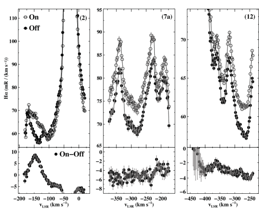
Figure 2: Sample on- and off-target WHAM spectra. The labels in the top-right corners coincide with the IDs used in Figure 1 and Table 1. The top half of the panels show an average of the on-target spectra as open circles and the average of the off-target spectra as filled circles, where the on and off observations were spaced $4\fdg 9$, $3\fdg 2$, and $2\fdg 9$ apart for the (2), (7a), and (12) sight lines, respectively. The bottom half of each panel shows the subtraction of the off-target spectra from the on-target spectra. Some of the atmospheric lines are many times brighter than the weaker emission from the Stream, such as the H$\alpha$ geocoronal line located at ${{\rm v}_{\rm{LSR}}}\approx-25~{}{\rm km\thinspace s^{-1}}$ for sight line (2).

The detection of diffuse optical-emission lines from the Stream, or from other high-velocity clouds (HVCs), requires very high surface brightness sensitivity and sufficient spectral resolution to differentiate it from local Galactic emission. The WHAM telescope is optimized to detect faint emission from diffuse, ionized sources with its high-throughput, $15~{}\,\mathrm{cm}$ diameter, dual-etalon Fabry-Pérot spectrometer that is coupled to a $0.6~{}{\rm m}$ objective lens (Reynolds et al. 1998b). We achieve a sensitivity of $\sim 30~{}{\rm mR}$, assuming a $30~{}{\rm km\thinspace s^{-1}}$ line width. Each individual exposure produces one spatially averaged spectrum that is $200~{}{\rm km\thinspace s^{-1}}$ wide with a spectral resolution of $12~{}{\rm km\thinspace s^{-1}}$ (${\rm R}\approx 25,000$) within the telescope’s $1\arcdeg$ beam. The ${\rm SF_{6}}$ pressure-controlled etalons and interference filters enable the spectra to be centered at any wavelength between $4800~{}\AA$ and $7300~{}\AA$. The WHAM telescope and its capabilities are described further in Haffner et al. (2003). Despite the large declination range, all of our observations were collected with the same facility. Positions (1)–(19) were targeted while WHAM was located at Kitt Peak National Observatory (KPNO; 1997–2007). It was then relocated to Cerro Tololo Inter-American Observatory (CTIO; 2009–present). From this current site, we observed the southern-hemisphere targets, (a)–(s).

From 2001–2008 at KPNO, we acquired $22$ targeted H$\alpha$ observations and complimentary off-target observations of the Magellanic Stream $50\arcdeg$ to $100\arcdeg$ from the MCs. These sight lines are labeled ($1-19$) under the ID column in Tables 1 and 2, which includes $3$ sight line pairs labeled “a” and “b” that substantially overlap. Figure 2 illustrates the on- and off-target observations along three sight lines and the results of their subtraction. Toward three of these $22$ sight lines, we also observed [S ii]$~{}\lambda 6716$, and [N ii] $\lambda 6583$ as well as [O ii]$~{}\lambda 7320$ and [O iii]$~{}\lambda 5007$ toward one sight line (see Table 3). These multiline spectra are shown in Figures 3–5. The H$\alpha$ intensities for these $22$ sight lines were first presented in BMS13 in their Figure 2. We have since reanalyzed their dataset and list updated values for the emission-line fits in Table 2.

We collected $17$ more targeted H$\alpha$, [S ii]$~{}\lambda 6716$, and [N ii] $\lambda 6583$ observations of the Stream from 2011–2013 at CTIO, which are labeled with IDs (a–s). Toward positions (a) and (e)—located near the MCs and only 8.2-degrees apart—we also observed the H$\beta$, [N ii]$~{}\lambda 5755$, [O i]$~{}\lambda 6300$, [O ii]$~{}\lambda 7320$, [O iii]$~{}\lambda 5007$, and He i$~{}\lambda 5876$ lines; these two sight lines probe two separate filaments of the Magellanic Stream with distinct velocities (Nidever et al. 2008) and different metallicities (Gibson et al. 2000; Fox et al. 2010, 2013; Richter et al. 2013). These multiline spectra are shown in Figures 6 and 7.

We observed each sight line for a total-integrated-exposure time of $5-50~{}{\rm minutes}$ with each filter. Each of the individual exposures lasted $60-300$ seconds (see Table 1). We alternated between on-target exposures with off-target exposures of the same length. These brief, individual exposures minimize the subtle changes in atmospheric emission that occur over short time scales. Although off-target sight lines that are positioned close to the on-target direction minimize the atmospheric differences between observations, FWB14 found that the ionized gas of the Stream can extend as much as $30\arcdeg$ off the H i emission. We therefore chose $2-3$ off-target directions per on-target, each positioned within $2-10~{}{\rm degrees}$ of the target and the H i emission; because our emission-line observations are less sensitive to low column density gas than the FWB14 absorption-line observations (our sensitivity scales as the square of the density and theirs scales linearly with density), this offset tended to be sufficient. To ensure that all of the chosen off-target directions were off of the H$\alpha$ emitting regions of the Stream, we paired and subtracted all nearby off-target observations from each other. In a few of the sight lines that were originally selected to be off positions, we detected H$\alpha$ emission with kinematics consistent with the H i gas in that region of the Stream. These serendipitous on-target observations are labeled with the “Near” prefix in the Notes column of Table 1. Additionally, all of these observations were positioned at least $0\fdg 55$ away from bright foreground stars ($m_{V}<6~{}{\rm mag}$) to avoid the distortion they cause to the continuum.

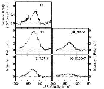
Figure 3: Multiline WHAM spectra along the BMS13 sight line labeled as (1) in Tables 1, 2, and 3. The H i spectrum is from the LAB Survey and was produced by averaging all the H i spectra within the WHAM beam.

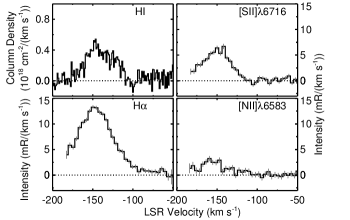
Figure 4: Same as Figure 3, but for the BMS13 sight line labeled as (2).

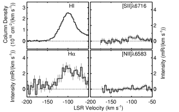
Figure 5: Same as Figure 3, but for the BMS13 sight line labeled as (3).

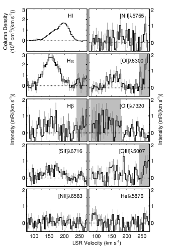
Figure 6: Same as Figure 3, but for the FAIRALL 9 sight line labeled as (a). Spectral regions highlighted in grey have diminished sensitivity due to increased residuals associated with bright atmospheric emission lines.

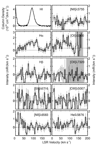
Figure 7: Same as Figure 3, but for the RBS 144 sight line labeled as (e). Spectral regions highlighted in grey have diminished sensitivity due increased residuals associated with bright atmospheric emission lines.

3 Reduction

3.1 Velocity and Intensity Calibration

We reduced the data with the WHAM pipeline (see Haffner et al. 2003). This is the same reduction procedure employed by Barger et al. (2012) in their HVC Complex A study that also utilized the WHAM telescope. Corrections to intensities were performed using synchronous observations of calibration targets, such as the North America Nebula (NGC 7000) that has an $I_{H\alpha}=850\pm 50~{}{\rm R}$ within a $50\arcmin$ beam (Scherb 1981 and Haffner et al. 2003). For the H$\alpha$ observations taken at KPNO, we also used these calibration target observations to correct for atmospheric transmission and to register the velocity frame. The procedures described below outline the velocity calibration and atmospheric line subtraction for all other data. To check for changes in instrumental throughput and to calibrate the surface brightness of the observations taken at CTIO, we compared the intensity of the H ii region surrounding $\lambda$ Orionis with data taken at both observing sites.

Roughly $20\%$ of our observations are contaminated by either the bright geocoronal H$\alpha$ line or strong OH molecular lines. These bright atmospheric lines lie at constant and well established velocities in the geocentric (GEO) frame (e.g., Hausen et al. 2002) with the geocoronal line at ${v_{\mathrm{GEO}}}=-2.3~{}{\rm km\thinspace s^{-1}}$ and a bright OH line lies at ${v_{\mathrm{GEO}}}=+272.44~{}{{\rm km\thinspace s^{-1}}}$ relative to the H$\alpha$ recombination line at $6562.8~{}\AA$. The presence of these lines enables us to calibrate the velocity extremely accurately. These bright lines also introduce more Poisson noise and typically lower our sensitivity by $10~{}{\rm mR}$, assuming a line width of $30~{}{\rm km\thinspace s^{-1}}$.

For spectra devoid of bright atmospheric contamination, we adopt an alternative method for their velocity calibration. To tune the wavelength center of WHAM’s spectroscopic window, we adjust the index of refraction of the gas located between WHAM’s Fabry-Pérot etalons by adjusting the gas pressure. The $\Delta\lambda$ varies linearly with the gas pressure (Tufte 1997). By monitoring the gas pressure, we can therefore determine the radial velocity of the emission by measuring its Doppler shift as this linear relationship is well-measured for the WHAM spectrograph. This is essentially the reverse of the tuning process described by Haffner et al. (2003) and is accurate to $\lesssim 5~{}{\rm km\thinspace s^{-1}}$ (Madsen 2004), though the relative velocities calibration of observations taken with different pressures but a the same interference order will agree within $0.1~{}{\rm km\thinspace s^{-1}}$ of each other.

3.2 Atmospheric Subtraction

When present, the bright geocoronal H$\alpha$ and OH molecular atmospheric lines dominate over the emission of the Magellanic Stream and faint atmospheric lines, with strengths that are often more than an order of magnitude greater (see Figure 3 of Barger et al. 2013). These bright lines are produced in Earth’s upper atmosphere from interactions with solar radiation. Therefore, their strength varies with both direction on the sky and the time of the observations. The difference in emission strength between these bright lines in the on- and off-target observations is much larger than the strength of the faint diffuse astronomical targets in this study. For these reasons, we first removed these bright lines from each exposure before subtracting the off-target observations from the on-target observations by modeling their shape as a single Gaussian convolved with the instrument profile of WHAM.

Once the bright atmospheric lines have been removed, we combine each set of individual ${\rm on}-{\rm off}$ target pairs by weighting their intensities and uncertainties with the number of observations in each velocity bin. Figure 2 illustrates average on- and off-target spectra as well as the resultant spectra after the on-off subtraction. Most of the observations were only affected by faint atmospheric emission lines. The surface brightness of these faint atmospheric lines exhibit spatial and temporal variations of up to $\sim 50\%$ throughout a single night, but are typically on the order of $\sim 0.1~{}{\rm R}$. Barger et al. (2013) list the atmospheric lines that contaminate the H$\alpha$ spectra at CTIO over the $-40~{}{\rm km\thinspace s^{-1}}\lesssim{v_{\mathrm{GEO}}}\lesssim+310~{}{\rm km\thinspace s^{-1}}$ velocity range in their Table 1 and they illustrate them in their Figure 3. Hausen et al. (2002) list these lines for KPNO over a shifted velocity window in their Table 3 and illustrate them in their Figures 1 and 2. Similar faint atmospheric lines contaminate all of the observations taken over the other wavelengths observed in this study. We isolate the astronomical emission by subtracting off-target observations from on-target observations, which substantially removes the fainter atmospheric contamination. We then remove the background continuum level by assuming a flat or linear background over all velocities. Slight differences in the continuum level in the reanalysis of the BMS13 dataset has resulted in a $\sim 10-20\%$ reduction in $I_{\rm H\alpha}$ from the values found in Figure 2 of their study.

3.3 Line Fitting

To measure the line strength and characteristics, we employed the Levenberg-Marquardt iteration technique (see Moré 1978) to calculate the fit parameters of a Gaussian convolved with the WHAM instrument profile using $\widetilde{\chi}^{2}$ minimization with the MPFIT IDL routine (Markwardt 2009). A second Gaussian was used only when the data could not be reasonably fit with one Gaussian such that the reduced $\widetilde{\chi}_{\rm min}^{2}$ exceeded $2.5$. For example, although a second Gaussian fit could be imposed to align with the sharp peak at $\sim 120~{}{\rm km\thinspace s^{-1}}$ along sight line (e), at an offset of only $\sim 15~{}{\rm km\thinspace s^{-1}}$ from the H i center; however, this peak is quite narrow and uncharacteristic of typical warm ionized gas emission line profiles. Although we could improve our fits further through the inclusion of more Gaussians, each spectrum represents an average of all component structure contained within the observed $1\arcdeg$ beam, which corresponds to a physical diameter of $\sim 1~{}\,\mathrm{kpc}$ near the Magellanic Clouds and up to $\sim 3.5~{}\,\mathrm{kpc}$ at the trailing tip of the Stream where its distance its predicted to lie between $55-200~{}\,\mathrm{kpc}$ from the Galactic Center (see Section 1). Additional components would not necessarily result in a disentanglement of that structure. This means that kinematically the resultant spectral lines become substantially broadened by unresolved non-thermal motions (e.g., bulk motion, larger scale turbulence, shear, rotation, etc.) of the gas contained within the large WHAM beam.

The results of the H$\alpha$ and H i data fits and their corresponding $\widetilde{\chi}_{\rm min}^{2}$ values and their corresponding $1\sigma$ statistical uncertainties are listed in Table 2 and in Table 3 for the multiline observations. In Table 2, we also include a spread of intensities that have a $\widetilde{\chi}^{2}$ that lie within $10\%$ of the $\widetilde{\chi}_{\rm min}^{2}$. This was included because for some of our spectra there was insufficient continuum surrounding the emission line to adequately anchor its level and slope, which translated to a wider range of parameters that could describe the line profile well. We represented this as ${\rm best~{}fit~{}I_{\rm H\alpha}}\pm{\rm 1\sigma}^{+\rm spread}_{-\rm spread}$ in Table 2. For example, the best fit H$\alpha$ intensity for sight line (a) is $165\pm 8~{}{\rm mR}$ with ${\widetilde{\chi}}_{\rm min}^{2}=1.0$ and the range of intensities with ${\widetilde{\chi}}^{2}\leq 1.1\widetilde{\chi}_{\rm min}^{2}$ is $104\leq I_{\rm H\alpha}\leq 190~{}{\rm mR}$.

We report upper limits for the multiline WHAM observations and H i column densities in Tables 2 and 3 if the line strength does not exceed a $3\sigma$ detection. For the H i upper limits, we equate this significance as three times the standard deviation of the scatter in the background over a fixed line width of $30~{}{\rm km\thinspace s^{-1}}$. For the WHAM dataset, we calculate this upper limit using the width of the H i emission or as $30~{}{\rm km\thinspace s^{-1}}$ in the absence of a H i detection. Note that because the gas phase traced by the WHAM observations is generally warmer than the H i gas, their actual line widths are expected to be larger than the H i. We find that FWHM of the H$\alpha$ emission in the Magellanic Stream is typically $\sim 55~{}{\rm km\thinspace s^{-1}}$ compared to $\sim 35~{}{\rm km\thinspace s^{-1}}$ for the H i (Table 2). Although the H$\alpha$ width is typically $1.6$ times that of the H i emission, there is likely unresolved multi-component substructure in the H$\alpha$ emission within the 1-degree WHAM beam ($\sim 1~{}\,\mathrm{kpc}$ at 55 $\,\mathrm{kpc}$) that would broadens the emission as suggested in spectra of sight lines (e) and (k).

3.4 Extinction Correction

Lastly, we apply the extinction correction procedure used by Barger et al. (2013) to correct the intensity attenuation caused by the foreground dust in the MW. Fox et al. (2013) found that the depletion of the low- and high-metallicity filaments of the Magellanic Stream primarily varies with the strength of the H i column density ($N_{\rm H\textsc{~{}i}}$) and not with the metallicity. Therefore, the self extinction is negligible in low H i column density regions of the Stream. Among our sample, only $5/39$ sight lines have $\log N_{\rm H\textsc{~{}i}}/\,\mathrm{cm}^{-2}\geq 20$ and for those sight lines, the self extinction correction is only $\lesssim 1-2\%$ for these sight lines.

This extinction correction is smallest when the Stream lies significantly above or below the Galactic plane ($\lvert b\rvert\gtrsim 25\arcdeg$). The correction substantially increases near the Galactic disk ($\lvert b\rvert\lesssim 25\arcdeg$). To correct the attenuated intensities, we use the excess color presented by Diplas & Savage (1994) for a warm diffuse medium:

$$E(B-V)=\frac{\langle N_{\rm H{~{}\textsc{i}}}\rangle}{4.93\times 10^{21}~{}\mathrm{atoms\cdot cm^{-2}\cdot mag^{-1}}}$$ (1)

where $N_{\rm H{~{}\textsc{i}}}$ only includes the foreground Galactic H i emission (Bohlin et al. 1978) and is calculated using the average of Leiden/Argentine/Bonn Galactic H i survey (LAB: Kalberla et al. 2005; Hartmann & Burton 1997) spectra within the WHAM 1-degree beam over the $-150\leq{{\rm v}_{\rm{LSR}}}\leq+150~{}{\rm km\thinspace s^{-1}}$ velocity range. We assume that the extinction follows the $\langle A(\mathrm{H}\alpha)/A(V)\rangle=0.909-0.282/R_{v}$ optical curve presented in Cardelli et al. (1989) for a diffuse interstellar medium, where R${}_{v}\equiv A(V)/E(B-V)=3.1$, so the expression for the total extinction becomes

$$A(\mathrm{H}\alpha)=6.3\times 10^{-22}~{}\langle N_{\rm H{~{}\textsc{i}}}\rangle~{}\mathrm{cm^{2}\cdot atoms^{-1}\cdot mag}.$$ (2)

The extinction corrected intensity for Galactic attenuation is then $I_{\mathrm{H}\alpha,~{}corr}=I_{\mathrm{H}\alpha,~{}obs}~{}e^{\ A(\mathrm{H}\alpha)/2.5}$, where $1.03\leq e^{\ A(\mathrm{H}\alpha)/2.5}\leq 1.14$ for all sight lines in this study.

Only for the sight line toward Fairall 9 at position (a), we include a correction for Magellanic Stream attenuation but only for the $I_{\rm H\alpha}/I_{\rm H\beta}$ ratio as these lines have a large difference in wavelength. Along this sight line, we detect both H$\alpha$ and H$\beta$ at $165\pm 8~{}{\rm mR}$ and $33\pm 9~{}{\rm mR}$ (non-extinction corrected; see Figure 6) yielding an extinction corrected ratio of $I_{\rm H\alpha}/I_{\rm H\beta}=5.0\pm 1.4$. As the FAIRALL 9 sight line lies along the high metallicity filament (Richter et al. 2013), we corrected for self extinction using the average LMC extinction curves of Gordon et al. (2003). As these lines trace the same ionization conditions (i.e., density and temperature) and do not depend on metallicity, their ratio is often used to measure the amount of reddening due to dust extinction. Although this value is larger than the nominal value of $\sim 3$, implying the presence of dust, slow shocks could also elevate the H$\alpha$ emission and increase this ratio beyond $4$ (Chevalier & Raymond 1978; Shull & McKee 1979; Bland-Hawthorn et al. 2007). This large ratio suggests that this gas is also being collisionally ionized. Unfortunately, due to the low signal-to-noise ratio of the H$\beta$ detection and the lack of detections toward other sight lines, we are unable to confidently determine the source of this enhancement. In the analysis below, we only correct our observations for extinction due to the foreground dust in the MW.

Table 2: H$\alpha$ and H i Line Fitting Results

	H$\alpha$					H i				position
ID	$I_{\rm H\alpha}$	${{\rm v}_{\rm{LSR}}}$	FWHM	$\widetilde{\chi}^{2}$		$\log{\rm N}_{\rm H\textsc{~{}i}}/\,\mathrm{cm}^{-2}$	${{\rm v}_{\rm{LSR}}}$	FWHM	$\widetilde{\chi}^{2}$
	(mR)	(${\rm km\thinspace s^{-1}}$)	(${\rm km\thinspace s^{-1}}$)				(${\rm km\thinspace s^{-1}}$)	(${\rm km\thinspace s^{-1}}$)
a	$165\pm 8^{+25}_{-61}$	$158\pm 1$	$67\pm 2$	$1.1$		$19.48\pm 0.01^{+0.06}_{-0.11}$	$158\pm 1$	$40\pm 1$	$1.0$	on, FAIRALL 9
a						$19.85\pm 0.01^{+0.07}_{-0.02}$	$200\pm 1$	$38\pm 1$	$1.0$	on, FAIRALL 9
b	$69\pm 5^{+26}_{-65}$	$135\pm 5$	$79\pm 5$	$1.0$		$<18.67$	$+135$	$\cdots$	$\cdots$	edge, Near HE0226-4110
c	$53\pm 9^{+24}_{-19}$	$150\pm 6$	$74\pm 12$	$1.4$		$17.05\pm 0.04$	$+165$	$\cdots$	$\cdots$	off, HE0226-4110
d	$53\pm 10^{+15}_{-24}$	$102\pm 3$	$54\pm 6$	$1.6$		$19.38\pm 0.01^{+0.01}_{-0.01}$	$135\pm 1$	$28\pm 1$	$1.0$	on-small, Near RBS 144
e	$101\pm 9^{+19}_{-22}$	$87\pm 3$	$79\pm 5$	$1.0$		$19.93\pm 0.01^{+0.01}_{-0.01}$	$93\pm 1$	$26\pm 1$	$1.0$	off, RBS 144
e						$18.95\pm 0.02^{+0.12}_{-0.07}$	$117\pm 1$	$25\pm 1$	$1.0$	off, RBS 144
f	$57\pm 11^{+16}_{-12}$	$99\pm 3$	$50\pm 3$	$1.2$		$19.06\pm 0.02^{+0.01}_{-0.01}$	$94\pm 1$	$29\pm 1$	$1.1$	edge, Near RBS 144
g	$<45$	$\cdots$	$\cdots$	$\cdots$		$<18.59$	$+210$	$\cdots$	$\cdots$	off, HE0153-4520
h	$105\pm 21^{+42}_{-40}$	$109\pm 2$	$61\pm 6$	$1.9$		$18.63\pm 0.04^{+0.01}_{-0.01}$	$92\pm 2$	$32\pm 2$	$1.1$	off, Near RBS 1892
j	$<49$	$\cdots$	$\cdots$	$\cdots$		$<18.78$	$+200$	$\cdots$	$\cdots$	off, ESO292-G24
k	$101\pm 22^{+35}_{-48}$	$117\pm 6$	$80\pm 7$	$1.0$		$18.76\pm 0.01$	$+125\pm 1$	$34\pm 7$	$1.3$	edge, Near HE0056-3622
m	$69\pm 3^{+16}_{-21}$	$-133\pm 2$	$52\pm 1$	$1.0$		$18.74\pm 0.04^{+0.01}_{-0.01}$	$-132\pm 2$	$47\pm 3$	$1.0$	off, Near PHL2525
n	$<37$	$\cdots$	$\cdots$	$\cdots$		$<18.83$	$-135$	$\cdots$	$\cdots$	edge-small, PHL2525
o	$<25$	$\cdots$	$\cdots$	$\cdots$		$<18.83$	$-150$	$\cdots$	$\cdots$	off, UM239
p	$<30$	$\cdots$	$\cdots$	$\cdots$		$<18.82$	$-250$	$\cdots$	$\cdots$	edge, NEAR NGC7714
q	$<31$	$\cdots$	$\cdots$	$\cdots$		$<18.85$	$-200$	$\cdots$	$\cdots$	off, MRK 1502
r	$<34$	$\cdots$	$\cdots$	$\cdots$		$<18.76$	$-200$	$\cdots$	$\cdots$	off, MRK 304
s	$162\pm 31^{+62}_{-84}$	$-328\pm 3$	$92\pm 8$	$1.9$		$16.67\pm 0.02$	$-300$	$\cdots$	$\cdots$	off, MRK 335
1						$18.78\pm 0.01^{+0.11}_{-0.09}$	$-146\pm 1$	$26\pm 1$	$1.0$	on
1	$417\pm 1^{+17}_{-14}$	$-121\pm 1$	$50\pm 1$	$2.1$		$19.14\pm 0.01^{+0.10}_{-0.05}$	$-118\pm 1$	$30\pm 1$	$1.0$	on
2	$574\pm 17^{+1}_{-21}$	$-141\pm 1$	$52\pm 1$	$1.1$		$19.17\pm 0.02^{+0.09}_{-0.05}$	$-148\pm 1$	$30\pm 1$	$1.3$	edge
2						$18.83\pm 0.02^{+0.12}_{-0.09}$	$-121\pm 1$	$18\pm 1$	$1.1$	edge
3	$108\pm 27^{+53}_{-102}$	$-100\pm 4$	$64\pm 4$	$1.0$		$20.03\pm 0.01^{+0.01}_{-0.01}$	$-101\pm 1$	$40\pm 1$	$1.0$	on
4a	$<50$	$\cdots$	$\cdots$	$\cdots$		$20.02\pm 0.01^{+0.01}_{-0.04}$	$-109\pm 1$	$34\pm 1$	$1.0$	on
4b	$66\pm 18^{+17}_{-12}$	$-107\pm 3$	$44\pm 6$	$1.0$		$20.01\pm 0.01^{+0.03}_{-0.04}$	$-110\pm 1$	$34\pm 1$	$1.0$	on
5a	$138\pm 23^{+50}_{-45}$	$-163\pm 2$	$82\pm 9$	$1.1$		$19.65\pm 0.01^{+0.09}_{-0.04}$	$-155\pm 1$	$45\pm 1$	$1.0$	on
5b	$122\pm 6^{+19}_{-27}$	$-173\pm 2$	$45\pm 1$	$1.0$		$19.56\pm 0.01^{+0.04}_{-0.12}$	$-159\pm 1$	$34\pm 1$	$1.0$	on
6	$110\pm 11^{+26}_{-24}$	$-134\pm 2$	$75\pm 6$	$1.4$		$19.73\pm 0.01^{+0.08}_{-0.04}$	$-158\pm 1$	$56\pm 1$	$1.0$	on
7a	$77\pm 16^{+17}_{-13}$	$-202\pm 2$	$45\pm 3$	$1.5$		$19.96\pm 0.01^{+0.01}_{-0.01}$	$-211\pm 1$	$29\pm 1$	$1.5$	edge
7a						$19.06\pm 0.02^{+0.07}_{-0.08}$	$-179\pm 1$	$27\pm 1$	$1.5$	edge
7b	$112\pm 19^{+19}_{-21}$	$-189\pm 2$	$72\pm 3$	$1.2$		$19.93\pm 0.01^{+0.01}_{-0.01}$	$-211\pm 1$	$31\pm 1$	$1.0$	edge
7b						$19.49\pm 0.01^{+0.05}_{-0.03}$	$-182\pm 1$	$35\pm 1$	$1.5$	edge
8	$50\pm 6^{+24}_{-36}$	$-197\pm 5$	$78\pm 8$	$1.0$		$19.58\pm 0.02^{+0.01}_{-0.02}$	$-217\pm 1$	$29\pm 1$	$1.9$	on
8						$18.97\pm 0.02^{+0.06}_{-0.03}$	$-219\pm 3$	$27\pm 2$	$1.0$	on
9	$104\pm 22^{+23}_{-47}$	$-238\pm 2$	$49\pm 1$	$1.0$		$19.60\pm 0.01^{+0.13}_{-0.01}$	$-227\pm 1$	$63\pm 1$	$1.0$	on
10	$152\pm 5^{+32}_{-69}$	$-231\pm 1$	$61\pm 1$	$1.0$		$19.68\pm 0.01^{+0.08}_{-0.06}$	$-231\pm 1$	$45\pm 1$	$1.0$	on
11	$<30$	$\cdots$	$\cdots$	$\cdots$		$19.22\pm 0.01^{+0.07}_{-0.09}$	$-300\pm 1$	$32\pm 1$	$1.4$	on
12	$64\pm 10^{+9}_{-11}$	$-354\pm 3$	$66\pm 5$	$1.3$		$19.49\pm 0.01^{+0.05}_{-0.05}$	$-361\pm 1$	$35\pm 1$	$1.5$	on
13	$30\pm 5^{+15}_{-30}$	$-317\pm 4$	$49\pm 6$	$1.0$		$19.07\pm 0.02^{+0.09}_{-0.16}$	$-317\pm 2$	$64\pm 3$	$1.0$	on
14	$59\pm 5^{+25}_{-27}$	$-332\pm 4$	$74\pm 5$	$1.0$		$19.17\pm 0.02^{+0.06}_{-0.10}$	$-322\pm 1$	$24\pm 1$	$1.0$	on
14						$19.14\pm 0.01^{+0.08}_{-0.09}$	$-354\pm 1$	$22\pm 1$	$1.0$	on
15	$34\pm 6^{+13}_{-39}$	$-319\pm 4$	$46\pm 2$	$1.0$		$19.23\pm 0.01^{+0.06}_{-0.03}$	$-323\pm 1$	$27\pm 1$	$1.2$	on
15						$18.77\pm 0.03^{+0.06}_{-0.11}$	$-351\pm 1$	$27\pm 1$	$2.4$	on
16	$<50$	$\cdots$	$\cdots$	$\cdots$		$18.92\pm 0.01^{+0.08}_{-0.04}$	$-321\pm 1$	$31\pm 1$	$1.0$	edge
17	$<34$	$\cdots$	$\cdots$	$\cdots$		$<18.85$	$-320$	$\cdots$	$\cdots$	off
18	$<50$	$\cdots$	$\cdots$	$\cdots$		$<18.82$	$-320$	$\cdots$	$\cdots$	off
19	$60\pm 9^{+12}_{-18}$	$-331\pm 2$	$59\pm 2$	$1.0$		$19.13\pm 0.01^{+0.10}_{-0.06}$	$-335\pm 1$	$26\pm 1$	$1.0$	on

Table 3: WHAM Multiline Fitting Results

ID	Line	I	${{\rm v}_{\rm{LSR}}}$	FWHM	$\widetilde{\chi}^{2}$
		(mR)	(${\rm km\thinspace s^{-1}}$)	(${\rm km\thinspace s^{-1}}$)
a	$\rm H\beta$	$33\pm 9$	$+158\pm 27$	$55\pm 25$	$0.9$
a	[S ii]$~{}\lambda 6716$	$36\pm 6$	$+164\pm 12$	$70\pm 14$	$85$
a	[N ii]$~{}\lambda 6583$	$<22$	$\cdots$	$\cdots$	$\cdots$
a	[N ii]$~{}\lambda 5755$	$<43$	$\cdots$	$\cdots$	$\cdots$
a	[O i]$~{}\lambda 6300$	$33\pm 8$	$+163\pm 14$	$56\pm 17$	$0.71$
a	[O ii]$~{}\lambda 7320$	$<39$	$\cdots$	$\cdots$	$\cdots$
a	[O iii]$~{}\lambda 5007$	$<36$	$\cdots$	$\cdots$	$\cdots$
a	He i	$<31$	$\cdots$	$\cdots$	$\cdots$
b–d	[S ii]$~{}\lambda 6716$	$\lesssim 40$	$\cdots$	$\cdots$	$\cdots$
b–d	[N ii]$~{}\lambda 6583$	$\lesssim 40$	$\cdots$	$\cdots$	$\cdots$
e	$\rm H\beta$	$<47$	$\cdots$	$\cdots$	$\cdots$
e	[S ii]$~{}\lambda 6716$	$<53$	$\cdots$	$\cdots$	$\cdots$
e	[N ii]$~{}\lambda 6583$	$<28$	$\cdots$	$\cdots$	$\cdots$
e	[N ii]$~{}\lambda 5755$	$<24$	$\cdots$	$\cdots$	$\cdots$
e	[O i]$~{}\lambda 6300$	$45\pm 8$	$+81\pm 15$	$54\pm 30$	$1.7$
e	[O ii]$~{}\lambda 7320$	$<38$	$\cdots$	$\cdots$	$\cdots$
e	[O iii]$~{}\lambda 5007$	$<52$	$\cdots$	$\cdots$	$\cdots$
e	He i$~{}\lambda 5876$	$<33$	$\cdots$	$\cdots$	$\cdots$
f–s	[S ii]$~{}\lambda 6716$	$\lesssim 40$	$\cdots$	$\cdots$	$\cdots$
f–s	[N ii]$~{}\lambda 6583$	$\lesssim 40$	$\cdots$	$\cdots$	$\cdots$
1	[S ii]$~{}\lambda 6716$	$140\pm 7$	$-130\pm 2$	$51\pm 3\phantom{0}$	$1.8$
1	[N ii]$~{}\lambda 6583$	$74\pm 10$	$-136\pm 6$	$67\pm 12$	$1.5$
1	[O i]$~{}\lambda 6300$	$<40$	$\cdots$	$\cdots$	$\cdots$
1	[O iii]$~{}\lambda 5007$	$<25$	$\cdots$	$\cdots$	$\cdots$
2	[S ii]$~{}\lambda 6716$	$230\pm 21$	$-151\pm 2$	$51\pm 3\phantom{0}$	$1.8$
2	[N ii]$~{}\lambda 6583$	$77\pm 16$	$-156\pm 4$	$45\pm 6\phantom{0}$	$1.0$
3	[S ii]$~{}\lambda 6716$	$<28$	$\cdots$	$\cdots$	$\cdots$
3	[N ii]$~{}\lambda 6583$	$<22$	$\cdots$	$\cdots$	$\cdots$

4 Comparison of Neutral and Ionized Gas

In this section, we compare the strength and velocity distribution of the H i and H$\alpha$ emission. The large and small scale similarities and differences between the neutral and ionized gas phases provide clues as to which astrophysical processes are affecting the Magellanic Stream. Some of these processes include photoionization from the surrounding radiation field and ram-pressure stripping from the Galactic halo, among others. Understanding their influence is critical to predict whether the neutral gas contained within the Stream can reach the disk and replenish the MW before it evaporates into the halo.

The Magellanic Stream extends over $165\arcdeg$ evident by its widespread H i emission that decreases steadily along its length (see Figures 1 and Figure 10 of Nidever et al. 2010). This Stream is composed of two spatially (Putman et al. 2003b) and kinematically (see Figure 13b of Nidever et al. 2008) distinct filaments. Each of these filaments has a different metallicity with one measured at $50\%~{}{\rm solar}$ toward only the FAIRALL 9 sight line (S ii/H=0.27 solar: Gibson et al. 2000; S/H=0.5 and N/H=0.07 solar: Richter et al. 2013) and the other at $10\%~{}{\rm solar}$ toward eight sight lines (Gibson et al. 2000; Fox et al. 2010, 2013). A gap between these two filaments is visible right above the (e-f) label in Figure 1.

Our targets lie on and off these two H i filaments. The right panels of Figures 8–11 include examples of the H i distribution surrounding $9$ of our $39$ sight lines. The locations of the WHAM observations within these representative gas distribution maps are marked with black hollow circles that are the size of our $1\arcdeg$ beam. The corresponding H$\alpha$ and H i spectra at these locations are displayed in the left panels of these figures. The Appendix includes the H$\alpha$ and H i spectra along all of our sight lines and two ${N}_{\rm H\textsc{~{}i}}$ maps showing distribution of the neutral gas around most of the sight lines that are not included in Figures 8–11.

4.1 $\rm H\alpha$ and $\rm H\textsc{~{}i}$ Emission Strengths and Kinematics

The strength of the H$\alpha$ emission along the Magellanic Stream does not vary with the H i column density (Figure 12). Differences in path lengths or filling factors between the neutral and ionized gas, as well as changes in the ionization fraction along these sight lines, could result in uncorrelated H i and H$\alpha$ emission strengths. On the other hand, the line centers of the H i and the H$\alpha$ emission are tightly correlated with an average separation of only $\langle|\Delta{\rm v}|\rangle=9.3~{}{\rm km\thinspace s^{-1}}$, though the H$\alpha$ emission tends to be $1.6\times$ broader than the H i emission (Figure 13). This correlation in their line centers suggests that the warm ionized and warm neutral gas responsible for the H$\alpha$ and H i emission are physically associated. If a single ionization process along the Stream were producing mixed, co-spatial regions of ionized and neutral gas, we would expect to see a correlation between the H$\alpha$ and H i emission. In this scenario, differences between the path lengths and/or densities along each sight lines would produce a range of intensities but the emission lines would be generally correlated. However, in regions studied so far, the strength of the H$\alpha$ and H i emission do not appear correlated despite having similar velocity centroids. In this case, the neutral and ionized phases are likely not well-mixed but are occurring within a distinct kinematic (and likely physical) region of the Stream. This behavior is also seen in IVCs and HVCs in the Milky Way that tend to have uncorrelated H$\alpha$ and H i emission strengths and correlated line centers (e.g., Haffner et al. 2001, Putman et al. 2003a, Haffner 2005, Hill et al. 2009, Barger et al. 2012, 2013). One straightforward configuration that may give rise to a kinematic association and lack of intensity correlation is if the ionization is occurring on the outside of a neutral cloud or on a side of neutral sheets. We discuss the source of the ionization in more detail in Section 5 below.

The sight lines with the largest offsets in H i and H$\alpha$ line centers tend to be toward regions faint in H i as is the case with sight line (d), which is illustrated in Figure 8; however, regions with low H i column densities do not always equate to large offsets as is the case with the sight line (b) as shown in Figure 10. Below we discuss a few representative examples of the differences and similarities between the H i and H$\alpha$ emission strengths and line centers along high and low H i column density regions.

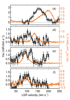
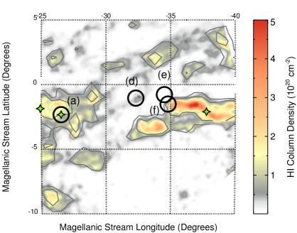
Figure 8: The H i column density map on the right shows the neutral gas distribution for the regions surrounding the FAIRALL 9 (a) and RBS 144 (e) sight lines. The H i (orange) and H$\alpha$ (black) spectra along the three targeted sight lines (a) and (d–f) are included on the left. The map and spectra labels coincide with the ones used in Figure 1 and Table 1. The binning of the H$\alpha$ spectra has been reduced from $2~{}{\rm km\thinspace s^{-1}}$ to $4~{}{\rm km\thinspace s^{-1}}$ to reduce residual systematics from very faint atmospheric lines in the spectra. The black circles in the H i map (right panel) represent the positions and coverage area of pointed WHAM observations used to produce the spectra in the left panel. The H i spectra within $1\arcdeg$ have been averaged together to match the WHAM observations. The H i spectra displayed in the left figure is from the LAB survey and was produced by averaging all the spectra within the WHAM beam. The map in the right figure displays the H i column density over the $+50\leq{{\rm v}_{\rm{LSR}}}\leq+250~{}{\rm km\thinspace s^{-1}}$ range from the GASS H i Survey with contour levels at $5\times 10^{19}$ and $10^{20}~{}{\,\mathrm{cm}^{-2}}$. The three green stars mark the locations of H$\alpha$ observations from PBV03.

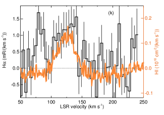
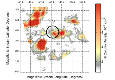
Figure 9: Same as Figure 8, but for the region surrounding the Near HE0056-3622 sight line labeled as (k). The map displays the H i column density from the GASS H i Survey over the $+100\leq{{\rm v}_{\rm{LSR}}}\leq+150~{}{\rm km\thinspace s^{-1}}$ range with contour levels at $10^{18}$ and $5\times 10^{18}~{}{\,\mathrm{cm}^{-2}}$.

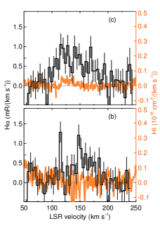
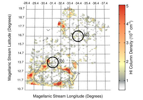
Figure 10: Same as Figure 8, but for the region surrounding the HE0226-4110 sight line labeled as (c). The map displays the H i column density from the GASS H i Survey over the range $+100\leq{{\rm v}_{\rm{LSR}}}\leq+200~{}{\rm km\thinspace s^{-1}}$ with contour levels at $1.5\times 10^{18}$ and $7\times 10^{18}~{}{\,\mathrm{cm}^{-2}}$. Although there is no detectable H i emission along these sight lines when averaged together to match the angular resolution of WHAM, only $2\arcdeg$ from the HE0226-4110 sight line (c) at $(-32\fdg 6,-17\fdg 9)$ there is emission with strength $4.5\times 10^{18}~{}\,\mathrm{cm}^{-2}$ centered at ${{\rm v}_{\rm{LSR}}}\approx+165~{}{\rm km\thinspace s^{-1}}$ and emission with strength $6\times 10^{18}~{}\,\mathrm{cm}^{-2}$ only $0.6\arcdeg$ away from sight line (b) at $(-30\fdg 9,-13\fdg 9)$ centered at ${{\rm v}_{\rm{LSR}}}\approx+135~{}{\rm km\thinspace s^{-1}}$ at the angular resolution of the GASS observations.

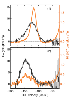
Figure 11: Same as Figure 8, but for the region surrounding the (1) and (2) BMS13 sight lines. The two green stars mark the locations of H$\alpha$ observations from PBV03 and the small light blue squares indicate the positions of the WVW02 and W03 observations. The map displays the H i column density from the GASS H i Survey over the $-250\leq{{\rm v}_{\rm{LSR}}}\leq-50~{}{\rm km\thinspace s^{-1}}$ range with contour levels at $10^{18}$ and $10^{19}~{}{\,\mathrm{cm}^{-2}}$.

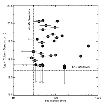
Figure 12: Comparison of the H$\alpha$ and H i (LAB H i Survey) emission, where H i spectra located within the 1-degree beam have been averaged together to yield same angular resolution. Error bars are shown in gray, with an arrow denoting the upper limit of a non-detection. The dashed lines denote the sensitivity of each survey to emission having $width=30~{}{\rm km\thinspace s^{-1}}$: WHAM, $I_{\rm H\alpha}\approx 30~{}{\rm mR}$ and $N_{\rm H{\textsc{~{}i}}}\approx 4.9\times 10^{18}~{}\,\mathrm{cm}^{-2}$.

Near the LMC at positions (e) and (f), we detect bright H$\alpha$ emission along the edge of the low metallicity Stream filament (see Figure 8). The H i and H$\alpha$ emission along these sight lines peak at roughly the same velocity. Sight line (e) lies off of the $\log{\rm N_{\rm H\textsc{~{}i}}/\,\mathrm{cm}^{-2}}=19$ contour and has an ${\rm N_{\rm H\textsc{~{}i}}}$ that is factor of seven less than sight line (f), which straddles the edge of this filament; however, the H$\alpha$ intensity decrease much more gradually, reducing only by a factor of $2$ (see Table 2). This small change in H$\alpha$ intensity with such a large change in H i column density suggests that the ionized gas extends much further than the neutral gas. This is consistent with the results of the Fox et al. (2014), which found that the ionized gas extends up to $30\arcdeg$ of the $\log{\rm N_{\rm H\textsc{~{}i}}/\,\mathrm{cm}^{-2}}=18$ gas when traced by UV absorption.

Numerous H i cloudlets are offset and moving with the main Magellanic Stream filaments, including one that intersects with sight line (d). The H$\alpha$ emission along this sight line lags behind the H i emission by roughly $30~{}{\rm km\thinspace s^{-1}}$ (see Figure 8 and Table 2), whereas the neutral and ionized gas at the nearby sight line (f), only 2-degrees away and on the edge of the H i filament, have a very similar velocity. However, as the kinematic span of the H$\alpha$ emission along the (d) and (f) sight lines is very similar, the large offset in the H i and H$\alpha$ line centroids along sight line (d) may indicate that the ionized and neutral gas are not well mixed.

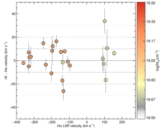
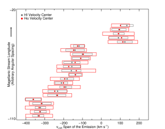
Figure 13: H$\alpha$ and H i kinematics. (Top) The offset of the H$\alpha$ line center from the H i with the symbol color representing the strength of the $N_{\rm H\textsc{~{}i}}$ emission. The horizontal lines at $0,~{}\pm 10,~{}\pm 20,and~{}\pm 30~{}{\rm km\thinspace s^{-1}}$ are provided for reference. (Bottom) The H$\alpha$ and H i LSR centroid position and the velocity spread of the lines. The vertical displacement follows the Magellanic Stream longitude at an arbitrary angular separation. The vertical sizes of the H$\alpha$ and H i rectangles are different only so that they are easier to visualize. The fit parameters of the H i lines were measured from LAB H i Survey spectra that were averaged together to match the WHAM angular resolution.

Toward a similarly detached cloud probed by sight line (k) positioned roughly $15\arcdeg$ downstream, we find that the kinematics of the neutral and ionized gas phase track each other well (see Figures 9 and 1). Though, it is also important to note that the cloud at position (k) might not actually be associated with the Magellanic Stream. The Sculptor Group of galaxies also lies in this general direction and at a similar velocity (e.g., Putman et al. 2003b). Fox et al. (2013) also detected this cloud at ${{\rm v}_{\rm{LSR}}}=+150~{}{\rm km\thinspace s^{-1}}$ through UV absorption and measured its oxygen abundance to be roughly a tenth solar; this abundance is very similar to the values they measure throughout the low metallicity filament of the Magellanic Stream. The ${{\rm v}_{\rm{LSR}}}=+125~{}{\rm km\thinspace s^{-1}}$ H$\alpha$ and H i emission along this sight line could therefore be associated with either the Magellanic Stream or the Sculptor Group.

Like the cloud at position (k), the sight lines at positions (1) and (2) also lie near $l_{\rm MS}=-50\arcdeg$, but on an offset cloud positioned at the low Magellanic Stream Latitude edge of an H i filament (see Figures 11 and 1). These two sight lines have an $I_{\rm H\alpha}$ that is $\sim 4-6$ times greater than sight line (k) positioned $8\arcdeg$ away and are over $200~{}{\rm mR}$ brighter than any of the other (a-s) and (3-19) sight lines presented in this study. Kinematically resolved mapped observations of the warm ionized gas in the Magellanic Stream are needed to ascertain why this portion of the Stream is so bright compared to the rest of the Stream and how well the neutral and ionized gas phases are mixed.

Although we generally detect H$\alpha$ emission on or near bright H i structures, we also detect ionized gas many degrees from the H i. Sight line (b) lies on the edge of multiple small H i clouds (Figure 10). At this location, the H i column density is below the sensitivity of the GASS H i survey, which is $N_{\rm H{\textsc{~{}i}}}=1.6\times 10^{18}~{}\,\mathrm{cm}^{-2}$ at a width of $30~{}{\rm km\thinspace s^{-1}}$ (McClure-Griffiths et al. 2009), but we detect warm ionized gas emission with $I_{\rm H\alpha}=69\pm 5~{}{\rm mR}$. Although this sight line lies $0\fdg 6$ from an H i cloud at $(l_{\rm MS},~{}b_{\rm MS})=(-30\fdg 9,-13\fdg 9)$, the H$\alpha$ emission lines up exceedingly well with the nearest sight line with detectible H i emission at ${{\rm v}_{\rm{LSR}}}\approx+135~{}{\rm km\thinspace s^{-1}}$ (see Table 2). Even further off these H i clouds, we detect H$\alpha$ emission along sight line (c) at $I_{\rm H\alpha}=53\pm 9~{}{\rm mR}$. Using H i Lyman series absorption, Fox et al. (2005) measured $\log{N_{\rm H\textsc{~{}i}}/\,\mathrm{cm}^{-2}}=17.05\pm 0.10$ over the $+80\leq{{\rm v}_{\rm{LSR}}}\leq+230~{}{\rm km\thinspace s^{-1}}$ velocity range using Far Ultraviolet Space Explorer (FUSE) observations with a pencil beam angular resolution; through photoionization modeling, they found that the Stream is more than $97\%$ ionized along this direction. At $2\arcdeg$ from this sight line at $(l_{\rm MS},~{}b_{\rm MS})=(-32\fdg 6,-17\fdg 9)$, the H i emission peaks $10~{}{\rm km\thinspace s^{-1}}$ from H$\alpha$ emission (${\rm v}_{\rm LSR,~{}H\alpha}\approx+155$ and ${\rm v}_{\rm LSR,~{}H\textsc{~{}i}}\approx+165~{}{\rm km\thinspace s^{-1}}$).

Overall, we find that the H$\alpha$ emission spatially tracks the H i emission of the Magellanic Stream well. In $4$ sight lines, we only detect H$\alpha$ emission, which indicates that the ionized gas has a larger cross section at the sensitivity of the WHAM ($\sim 30~{}{\rm mR}$) observations and the H i surveys (LAB: $4.9\times 10^{18}~{}\,\mathrm{cm}^{-2}$; GASS: $1.6\times 10^{18}~{}\,\mathrm{cm}^{-2}$). We also find that the strengths of these lines are not correlated (Figure 12), which suggests that the warm ionized gas phase ($10^{4}~{}{\rm K}$) is predominantly photoionized (see the discussion in this section above). The H i and H$\alpha$ velocity centroids agree well on the main H i Stream filaments, but less so for sight lines positioned off or on the cloudlets away from the main body of the Stream. This may indicate that clouds on the edge of the Stream are less shielded from their environment. However, the overall kinematic difference between the H i and H$\alpha$ centroids is centered at $\sim 0~{}{\rm km\thinspace s^{-1}}$ (see Figure 13).

4.2 Properties of the Ionized Gas

Table 4: Ionization Fraction from $N_{\rm H\textsc{~{}i}}$ and $I_{\rm H\alpha}$

	Observed			Modeled				Derived
ID	$\log N_{\rm H\textsc{~{}i}}/\,\mathrm{cm}^{-2}$	$I_{\rm H\alpha}$		$L$	$\chi_{\rm H\textsc{~{}ii}}$			$f_{\rm H\textsc{~{}ii}}$
		(mR)		($\,\mathrm{kpc}$)
a	$19.56\pm 0.01$ ($20.01\pm$0.01)	$165\pm 8$		$4$	$0.36$			$0.08-0.11$ $(0.15-0.22)\tablenotemark{c}$
e	$19.89\pm 0.01$ ($19.98\pm$0.02)	$101\pm 9$		$23$	$0.47$			$0.08-0.11$ $(0.09-0.13)\tablenotemark{c}$

To constrain how much H ii gas fills the WHAM beam and the fraction of ionized gas in the Magellanic Stream, we compared the H i, H$\alpha$, and [O i] emission with the UV absorption from the FWB14 study.

4.2.1 Filling Factor of the H ii Gas

The intensity of the H$\alpha$ emission is directly proportional to the rate of the recombination (Reynolds 1991):

$$I_{\rm H\alpha}=\frac{1}{2.75}~{}T_{4}^{-0.924}\left(\frac{\int{n_{e}^{2}}dl}{\rm cm^{-6}\ \,\mathrm{pc}}\right)~{}R,$$ (3)

where $T_{4}=\left(T_{e}/10^{4}~{}{\rm K}\right)$ with $T_{e}$ being the electron temperature of the gas. The $2.75^{-1}T_{4}^{-0.924}$ factor accounts for the rate of recombination and the subsequent probability of producing an H$\alpha$ photon in a gas optically thick to Lyman Continuum radiation (see Martin 1988 for these recombination coefficients). The integral term is known as the emission measure ($EM\equiv\int n_{e}^{2}dl$), where we have assumed that $n_{\rm H\textsc{~{}ii}}\approx n_{e}$. Here $n_{e}$ is the electron density and $dl$ is the line-of-sight path length over which the electrons are recombining.

Unfortunately, distribution of the electrons along the line of sight is unknown. A common approach is to parameterize the emission measure as $EM=n_{c}^{2}f_{\rm H\textsc{~{}ii}}L$, where $n_{c}$ now represents a characteristic electron density and $L$ is the path length of the emitting gas along the line of sight (e.g., Reynolds 1991). The fraction of the beam that is filled with gas is known as the filling factor ($f$) and is a dimensionless quantity that varies between $0\leq f\leq 1$. The product $fL$ is known the occupation length, which is the average portion of the line-of-sight depth that harbors gas. For a sight line in which the H i column density is known, we define the ionization fraction of hydrogen as $\chi_{\rm H\textsc{~{}ii}}=N_{\rm H\textsc{~{}ii}}/(N_{\rm H\textsc{~{}i}}+N_{\rm H\textsc{~{}ii}})$. Here, the column density of ionized hydrogen is then $N_{\rm H\textsc{~{}ii}}=\sqrt{EMf_{\rm H\textsc{~{}ii}}L}$, or $N_{\rm H\textsc{~{}ii}}=\sqrt{2.75I_{\rm H\alpha}T_{4}^{+0.924}f_{\rm H\textsc{~{}ii}}L}$ with equation (3) and assuming that $n_{p}\approx n_{e}$.

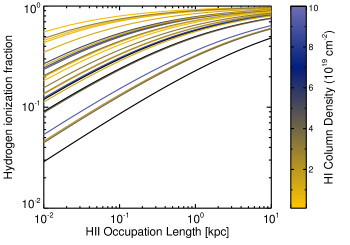
Figure 14: The $\chi_{\rm H\textsc{~{}ii}}$ trends (yellow-blue lines) for the $25$ sight lines (out of $39$) with detected H$\alpha$ and H i emission as a function of the H ii occupation length ($fL$), assuming $T_{4}=1$. The color of these lines illustrates the strength of the ${N_{\rm H\textsc{~{}i}}}$.

With the $N_{\rm H\textsc{~{}i}}$ and $I_{\rm H\alpha}$ detections alone, the occupation length is unconstrained. To illustrate how the occupation length varies with hydrogen ionization faction for our measured $N_{\rm H\textsc{~{}i}}$ and $I_{\rm H\alpha}$ along the Magellanic Stream, we assume $-2\leq\log\left(f_{\rm H\textsc{~{}ii}}L\right)\leq 1$ in Figure 14 such that the values span the $f_{\rm H\textsc{~{}ii}}=0.01$ and $L=1~{}\,\mathrm{kpc}$ to $f_{\rm H\textsc{~{}ii}}=1$ and $L=10~{}\,\mathrm{kpc}$ parameter space. For reference, at the distance of the Magellanic Clouds ($d_{\odot}\approx 55~{}\,\mathrm{kpc}$) the width of the $1\arcdeg$ WHAM beam corresponds to a projected physical width of $\sim 1~{}\,\mathrm{kpc}$; at the tip, the Stream might lie as far as $d_{\odot}\approx 100-200~{}\,\mathrm{kpc}$ as discussed in Section 1, which would correspond to a projected width of $\sim 1.7-3.5~{}\,\mathrm{kpc}$ for the WHAM beam. We find that over this $f_{\rm H\textsc{~{}ii}}L$ range, the $\chi_{\rm H\textsc{~{}ii}}$ would vary by factor of $10$ or more for small occupation lengths of $f_{\rm H\textsc{~{}ii}}L\lesssim 0.1~{}\,\mathrm{kpc}$ (Figure 14 and Table 2). The hydrogen ionization fraction begins to converge to $\chi_{\rm H\textsc{~{}ii}}\approx 1$ at $f_{\rm H\textsc{~{}ii}}L\gtrsim 100~{}\,\mathrm{kpc}$. Therefore, the combination of $N_{\rm H\textsc{~{}i}}$ and $I_{\rm H\alpha}$ is especially insensitive to the hydrogen ionization fraction at small occupation lengths. This is not too surprising that the combination of H i-21 $\,\mathrm{cm}$ and H$\alpha$ emission is inadequate for determining $f_{\rm H\textsc{~{}ii}}$ as the H i and H$\alpha$ emission are uncorrelated as illustrated in Figure 12. For comparison, FWB14 found that the hydrogen ionization fraction tends to increase with decreasing $N_{\rm H\textsc{~{}i}}$ for the low-ionization gas phase.

However, by combining our measurements of the H$\alpha$ and H i emission with UV absorption-line results on the Stream’s $L$ and $\chi_{\rm H\textsc{~{}ii}}$ from the FWB14 study, we can constrain the filling fraction of the ionized hydrogen:

$$f_{\rm H\textsc{~{}ii}}=\frac{1}{2.75I_{\rm H\alpha}T_{4}^{+0.924}L}\left(\frac{N_{\rm H\textsc{~{}i}}~{}\chi_{\rm H\textsc{~{}ii}}}{1-\chi_{\rm H\textsc{~{}ii}}}\right)^{2}$$ (4)

The FAIRALL 9 and RBS 144 sight lines at positions (a) and (e) overlap with the FWB14 sample. Table 4 lists the $\chi_{\rm H\textsc{~{}ii}}$ and $L$ found in the FWB14 study and the measured $I_{\rm H\alpha}$ and $N_{\rm H\textsc{~{}i}}$ values from this study for sight lines (a) and (e). Assuming a typical electron temperature of $[0.8-1.2]\times 10^{4}~{}{\rm K}$ in H$\alpha$ emitting regions (e.g., Madsen & Reynolds 2005; Madsen et al. 2006; FWB14 found that $T_{4}\approx 1$ through CLOUDY radiative transfer modeling), we find that $f_{\rm H\textsc{~{}ii}}=0.08-0.11$ along both sight lines. Table 4 summarizes these results.

Table 5: Ionization Fraction from $I_{\rm O\textsc{~{}i}}/I_{\rm H\alpha}$

	Observed				Derived		Modeled
ID	$\log N_{\rm H\textsc{~{}i}}/\,\mathrm{cm}^{-2}$	$I_{\rm H\alpha}$	$I_{\rm O\textsc{~{}i}}$		$\chi_{\rm H\textsc{~{}ii}}$		$\chi_{\rm H\textsc{~{}ii}}$
		(mR)	(mR)
a	$19.48\pm 0.01$	$165\pm 8$	$33\pm 8$		$0.16$, $0.32$, $0.47$		$0.30$
e	$19.93\pm 0.01$	$101\pm 9$	$45\pm 8$		$0.31$, $0.51$, $0.67$		$0.43$
1	$19.14\pm 0.02$	$417\pm 1$	$<40$		$<0.67$, $<0.83$, $<0.90$		$\cdots$

4.2.2 Ionization Fractions through $\rm H\alpha$ and $[\rm O\textsc{~{}i}]$

Unlike the $N_{\rm H\textsc{~{}i}}$ and $I_{\rm H\alpha}$ combination, the $\chi_{\rm H\textsc{~{}ii}}$ does not depend on the geometry of the emitting cloud when solved for using H$\alpha$ and [O i]$~{}\lambda 6300$. This is because the H$\alpha$ recombination line and collisionally excited [O i]$~{}\lambda 6300$ emission lines both trace the $n_{e}^{2}$ along the line of sight (i.e., $EM$). Assuming that this emission is from the same gas, their $f_{\rm H\textsc{~{}ii}}L$ and $n_{e}^{2}$ dependency cancels when taking their ratio (see Reynolds et al. 1998a; Hausen et al. 2002). As oxygen and hydrogen have very similar first ionization potentials, there is a strong charge-exchange reaction between the ground and first excited state of these elements. This couples their emission-line ratio to the ionization fraction of hydrogen (Field & Steigman 1971, Finkenthal et al. 1987, Domgorgen & Mathis 1994) such that $\chi_{\rm H\textsc{~{}ii}}$ is roughly inversely proportional to $I_{\rm[O\textsc{~{}i}]}/I_{\rm H\alpha}$ (Reynolds et al. 1998a and Hausen et al. 2002):

$$I_{\rm[O\textsc{~{}i}]}/I_{\rm H\alpha}= 2.74\times 10^{4}\frac{T_{4}^{1.854}}{1+0.605~{}T_{4}^{1.105}}e^{-2.284/T_{4}}$$

$$\times\left(\frac{\rm O}{\rm H}\right)\frac{1+n_{\rm H\textsc{~{}ii}}/n_{\rm H\textsc{~{}i}}}{[1+8/9n_{\rm H\textsc{~{}ii}}/n_{\rm H\textsc{~{}i}}]~{}n_{\rm H\textsc{~{}ii}}/n_{\rm H\textsc{~{}i}}}.$$ (5)

We detected both [O i] and H$\alpha$ along the low and high metallicity filament (see Figures 6 and 7). To determine the $\chi_{\rm H\textsc{~{}ii}}$ of the Stream, we assume that the oxygen gas phase abundance is $0.5~{}{\rm solar}$ for the FAIRALL 9 sight line at position (a) (Gibson et al. 2000; Richter et al. 2013) and $0.1~{}{\rm solar}$ for the RBS 144 sight line at position (e) and position (1) (Gibson et al. 2000; Fox et al. 2010, 2013) and electron gas temperatures of $T_{4}=[0.8,1,1.2]$. We also use the solar photospheric abundances of Asplund et al. (2009). Using equation 4.2.2, we find that $0.16\leq\chi_{\rm H\textsc{~{}ii}}\leq 0.47$ and $0.31\leq\chi_{\rm H\textsc{~{}ii}}\leq 0.67$ for FAIRALL 9 and RBS 144, respectively; these results are summarized in Table 5. These $\chi_{\rm H\textsc{~{}ii}}$ values closely agree with those found by FWB14 if $T_{4}\approx 1$, resulting in differences of only $6\%$ and $17\%$, suggesting the drastically different beam sizes sample similar ionization fractions even though the $N_{\rm H\textsc{~{}i}}$ varies within the WHAM beam.

5 Ionization Source of the Stream

The Magellanic Stream contains a substantial amount of ionized gas (e.g., Weiner & Williams 1996, Putman et al. 2003a, and Fox et al. 2005, 2014). Both photoionization and collisional ionization processes might contribute to the ionization of this structure. Sources of photoionization include the EGB (Bland-Hawthorn & Maloney 1999; Weymann et al. 2001; Haardt & Madau 2012), hot stars in the Milky Way and the Magellanic Clouds (i.e., MW: Fox et al. 2005; MCs: Barger et al. 2013), and potentially the Galactic Center. Sources of collisional ionization may include shocks, turbulent mixing, and conductive heating, which all may occur as the Stream interacts with the surrounding halo gas (e.g., Bland-Hawthorn et al. 2007; Putman et al. 2011; Joung et al. 2012). The region of the Stream that is below the South Galactic Pole (SGP) could also be susceptible to energetic events associated with the Galactic center, such as Fermi Bubbles (e.g., Su et al. 2010; Ackermann et al. 2014; Fox et al. 2015) and short lived Seyfert activity (see BMS13 and J. Bland-Hawthorn et al. 2017, in preparation).

5.1 Photoionization

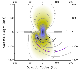
Figure 15: Ionizing radiation field ($\log{\left[\phi_{\rm{LC}}/{\rm photons}\ {\rm cm}^{-2}\ {\rm s}^{-1}\right]}$) for the MW (Fox et al. 2005) and the MCs (Barger et al. 2013) for a $400\times 400~{}\,\mathrm{kpc}$ slice through the center of the MW and LMC. The grayscale tracks assume that the Magellanic Stream is anchored at the center of the LMC ($d=50~{}\,\mathrm{kpc}$, $l_{\rm MS}=0\arcdeg$, $b_{\rm MS}=0\arcdeg$) and that it extends to $(d=50,~{}75,~{}100,~{}150~{}\,\mathrm{kpc},~{}l_{\rm MS}=-57\fdg 6,~{}b_{\rm MS}=0\arcdeg)$ below the SGP with a constant $\Delta d/\Delta l_{\rm MS}$ along its length. The purple line traces the Model 2 track from Besla et al. (2012), which places the Stream at $(l_{\rm MS},~{}b_{\rm MS},~{}d)=(-57\fdg 6,~{}0\arcdeg,~{}63~{}\,\mathrm{kpc}$) below the SGP and at $(-120\arcdeg,~{}0\arcdeg,~{}210~{}\,\mathrm{kpc}$) its tip.

As H$\alpha$ emission arises from the recombination of electrons and protons, the $I_{\rm H\alpha}$ is directly proportional to the rate of hydrogen ionizations per surface area of the emitting gas in local thermal dynamic equilibrium conditions (see Barger et al. 2012 for more details):

$$\phi_{\rm H\textsc{~{}i}\rightarrow H\textsc{~{}ii}}=2.1\times 10^{5}\left(\frac{{I_{\rm{H}\alpha}}}{0.1{\rm R}}\right)~{}T_{4}^{+0.118}~{}{\rm cm}^{-2}\ {\rm s}^{-1}.$$ (6)

If the ionization of an optically thick cloud is dominated by photoionization, then the incident Lyman Continuum flux ($\phi_{\rm LC}$) will be approximately equal to $\phi_{\rm H\textsc{~{}i}\rightarrow H\textsc{~{}ii}}$.

Weymann et al. (2001) predict that the background of ionizing radiation escaping from distant galaxies has a strength of $\phi_{\rm EGB}\approx 10^{4}~{}{\rm ionizing~{}photons}~{}\,\mathrm{cm}^{-2}~{}\,\mathrm{s}^{-1}$ at $z=0$. We approximate this ionizing background radiation as a constant flux along the entire Magellanic Stream, which produces enough ionization to elevate the H$\alpha$ emission of the Stream by $I_{\rm H\alpha}\approx 5~{}{\rm mR}$ (see Equation 6).

The amount of incident ionizing radiation along the Stream from nearby galaxies varies with its position with respect to those galaxies. The intensity of the ionizing radiation field of disk galaxies is generally expected to be greatest at their center where their stellar production is typically most intense. The amount of ionizing radiation escaping from the centers of these galaxies tends to decrease as the polar angle increases because the photons must travel through more interstellar medium to escape the galaxy. Therefore clouds positioned directly above or below the poles will experience the strongest ionizing flux. To estimate the contribution of ionizing photons that the Galaxy irradiates the Stream with, we use the Fox et al. (2005) model (an updated version of the Bland-Hawthorn & Maloney 1999, 2001 model), which has a vertical escape fraction ($f_{\rm esc}$) of $\sim 6\%$ over the poles and $\sim 1-2\%$ when averaged over a sphere. Although we also incorporated updated parameters for the Galactic corona from Miller & Bregman (2015), the UV emission from the halo remains negligible (i.e., a few percent at most) compared to the Galactic disk ($\phi_{\rm{LC}}\approx 10^{5}~{}{\rm photons}\ {\rm cm}^{-2}\ {\rm s}^{-1}$ at $50~{}\,\mathrm{kpc}$ along the SGP, corresponding to $I_{\rm H\alpha}\approx 50~{}{\rm mR}$ for $T_{4}=1$).

Near the MCs ($l_{\rm MS}>-30\arcdeg$), the ionizing radiation from the SMC and LMC cannot be neglected. We use the Barger et al. (2013) model of the ionizing radiation field emitted by the SMC and LMC to estimate their contribution. Based on an H$\alpha$ survey of the Magellanic Bridge, Barger et al. (2013) showed that the UV radiation from the Magellanic Clouds is sufficient to ionize the Magellanic Bridge, estimating $f_{\rm esc}\leq 5.5\%$ for the SMC and $f_{\rm esc}\leq 4.0\%$ for the LMC. Most of the ionizing flux that the Stream receives from these galaxies is from the LMC.

Due to the poorly constrained distance of the Magellanic Stream, its relative position with respect to the LMC, SMC, and MW is uncertain except for where the Stream originates (see Section 1). As the strength of the incident ionizing radiation field onto the Stream from these galaxies greatly depends its position, we compare the $I_{\rm H\alpha}$ with the Lyman continuum radiation field models over a wide range of distances. We therefore explore five different position tracks for the Stream that position it between $50-150~{}\,\mathrm{kpc}$ below the SGP at $l_{\rm MS}=-57\fdg 3$. Although it is well known that the Magellanic Stream originates from the MCs, it is uncertain where amongst these galaxies the longer of the two H i filament begins. Nidever et al. (2008) kinematically identified these two coherent filaments through component fitting of the H i emission spectra, but they were unable to determine if the longer filament traced back to the SMC, Magellanic Bridge, or the LMC. They were, however, able to determine that the shorter filament traces back to $30$ Doradus. We anchor four of our position tracks at the LMC ($d=50~{}\,\mathrm{kpc}$, $l=283\fdg 3$, $b=-32\fdg 4$), or ($d=50~{}\,\mathrm{kpc}$, $l_{\rm MS}=0\arcdeg$, $b_{\rm MS}=0\arcdeg$). For these tracks, we assume that the distance along the Stream changes linearly with angular distance; this assumption agrees well with galaxy interaction models for scenarios where the MCs are on their first-infall or are bound to the MW (e.g., Figure 3: Connors et al. 2006; Figure 10: Besla et al. 2012). We include a fifth track that follows the Stream positions that resulted from the $2^{\rm nd}$ LMC and SMC interaction model in Besla et al. (2012), which has the beginning of the Stream anchored at the Magellanic Bridge and not the LMC. The combined ionizing radiation field models for the MW, MCs, and EGB is shown in Figure 15 along with these five different position tracks for the Stream.

In Figure 16, we show how the strength of the $I_{\rm H\alpha}$ varies along the length of the Magellanic Stream. The horizontal axis indicates the angular distance from the LMC in Magellanic Stream coordinates (see Nidever et al. 2008), where $l_{\rm MS}=0\arcdeg$ crosses through the center of the LMC, $l_{\rm MS}\approx-17\arcdeg$ passes through the center of the SMC, and the grey shaded region spanning $-33\arcdeg\lesssim l_{\rm MS}\lesssim-81\arcdeg$ corresponds to cone with a half-opening angle of $\theta_{1/2}\approx 25\arcdeg$ which flares out from the Galactic center and is centered on the SGP at $(l_{\rm MS},~{}b_{\rm MS})=(-57\fdg 3,~{}+7\fdg 5)$. The right-hand y-axis includes an estimate for the rate of hydrogen ionizations per surface area of the Stream (see Equation 6). To test how well photoionization from the MW, MCs, and EGB alone can reproduce the H$\alpha$ emission in the Magellanic Stream, we illustrate the total $I_{\rm H\alpha}$ that is predicted from these ionization sources for our five position tracks shown in Figure 15. We show the ionizing contribution for the MW, MCs, and EGB separately in Figure 17. The ionizing contribution from the MCs drops off steeply between $-40\arcdeg\leq l_{\rm MS}\leq-20\arcdeg$, the MW’s contribution dominates above $l_{\rm MS}\geq-40\arcdeg$, while ionization from the EGB only produces a meager $I_{\rm H\alpha}\approx 5~{}{\rm mR}$ increase along the Stream. For all of the assumed distances, the average H$\alpha$ emission is roughly $50~{}{\rm mR}$ higher than anticipated from photoionization from these sources alone.

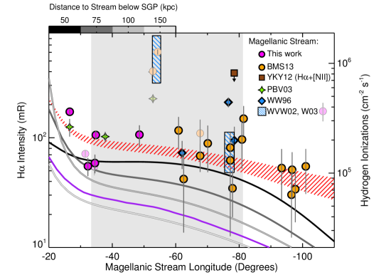
Figure 16: The H$\alpha$ intensities along the Magellanic Stream from this and the BMS13, YKY12, PBV03, WW96, WVW02, and W03 studies (detections only). The blue shaded polygons mark the ${\rm median}\pm{\rm average~{}deviation~{}from~{}the~{}median}$ for the WVW02 and W03 detections. Sight lines off of the H i filaments are colored in a lighter shade than indicated by the legend. The grey shaded region marks the portion of the Stream that lies within a $\theta_{1/2}=25\arcdeg$ cone that projects out from the Galactic Center along the SGP. The right-hand vertical axis marks the rate of hydrogen ionizations per surface area of the Stream that are needed to reproduce the H$\alpha$ emission (see Equation 6 for photoionization). The four black to light grey lines trace predicted photoionization due to the MW (Fox et al. 2005), LMC (Barger et al. 2013), and EGB (Weymann et al. 2001) for a Stream positioned at $(d=50,~{}75,~{}100,~{}150~{}\,\mathrm{kpc},~{}l_{\rm MS}=-57\fdg 6,~{}b_{\rm MS}=0\arcdeg)$ distance tracks as shown in Figure 15. The purple trace shows the predicted photoionization for Model 2 of Besla et al. (2012). The combined contribution from MW, MCs, and EGB photoionization and negligible halo-gas interactions (maximum contribution of $3~{}{\rm mR}$; BMS13) and shock-cascade self interactions (Tepper-García et al. 2015) is shown as a dashed red envelope for $n_{\rm halo}=2\times 10^{-4}~{}\,\mathrm{cm}^{-3}$ for the $d=75~{}\,\mathrm{kpc}$ track.

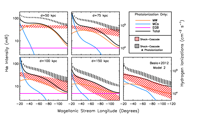
Figure 17: A breakdown of the anticipated H$\alpha$ intensity that results from each of the major sources of photoionization and collisional ionization for the five distance tracks shown in Figures 15 and 16. The corresponding number of hydrogen ionization from these sources is indicated in the right vertical axis (Figure 6). The photoionization contribution from the MCs is shown by the blue lines (Barger et al. 2013), the Milky Way by the orange lines (Fox et al. 2005), and the EGB by the pink lines (Weymann et al. 2001). The combined photoionization contribution from these three sources are the solid black lines. The estimated $I_{\rm H\alpha}$ that results from shock-cascade self interactions (Tepper-García et al. 2015) and halo-gas interactions (BMS13), respectively, for $n_{\rm halo}=2\times 10^{-4}~{}\,\mathrm{cm}^{-3}$ are shown as the red envelopes. The projected $I_{\rm H\alpha}$ that results from both the photoionization and collisional ionization combined are indicated by the black envelopes.

This leads us to a clear conclusion: photoionization from the MW, MCs, and the EGB alone is insufficient for producing the observed ionization in the Magellanic Stream.

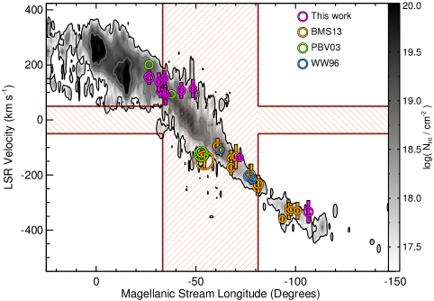
Figure 18: Position-velocity diagram of the H$\alpha$ detections along the Magellanic Stream. Symbol colors represent different studies, as in Figure 16. The size of the circles scale with the strength of the H$\alpha$ emission. The extent of the vertical colored bars signifying the width of the line (see Table 2), assuming a Gaussian distribution. The background map displays the H i column density of the Stream as a function of LSR velocity from the Nidever et al. (2008) Gaussian decompositions of the LAB survey. The vertical red shaded region spans the locations of the Stream positioned below the Galactic pole at $b\leq-65\arcdeg$ for $b_{\rm MS}=0\arcdeg$. The horizontal purple shaded region marks the velocities where confusion between the Magellanic Stream and MW is greatest.

5.2 Collisional Ionization

Collisional ionization from interactions with the Galactic halo and the Stream itself might be the cause of some of the elevated H$\alpha$ emission. Figure 18 illustrates how the H$\alpha$ emission varies along the Magellanic Stream with longitude and LSR velocity. The size of the multicolored circles in this figure scales with the $I_{\rm H\alpha}$ strength and the vertical bars signify the kinematic extent of the emission. The sight lines that are positioned spatially or kinematically off the two main H i filaments of the Stream are roughly $25~{}{\rm mR}$ brighter on average, excluding the brightest detections at $l_{\rm MS}\approx-55\arcdeg$ that will be discussed in Section 5.3 below. These sight lines probe locations on the Stream that are less shielded from their environment and are more exposed to the surrounding coronal gas and radiation field. In addition, limb brightening may result in a slightly higher $I_{\rm H\alpha}$ for sight lines that are projected spatially on the edge of the Stream.

There is now general concordance that the orbit of the Magellanic System is highly elliptical, which would place all but the portions of the Stream that are nearest to the MCs much further away (e.g., Besla et al. 2007; Jin & Lynden-Bell 2008; Guglielmo et al. 2014). Through ram-pressure modeling of the H i density profile of LMC’s disk, Salem et al. (2015) found that ${\rm n}_{\rm halo}\approx 10^{-4}~{}\,\mathrm{cm}^{-3}$ at $d\approx 50~{}\,\mathrm{kpc}$ would reproduce the observed compression in the disk’s leading edge. This density presumably drops with distance from the Milky Way, which will decrease the collisional interaction rate between the gas in the Stream with the surrounding coronal gas. Following the procedure employed in BMS13, we predict that halo-gas interactions will only marginally elevate the ionization in the Stream such that the $I_{\rm H\alpha}$ increases by $\leq 3~{}{\rm mR}$ (see their Equations 13 and A7-A12) when we spatially smooth their model to match the $1\arcdeg$ resolution of WHAM for a Stream positioned $d=75~{}\,\mathrm{kpc}$ below the SGP and assume ${\rm n}_{\rm halo}=2\times 10^{-4}~{}\,\mathrm{cm}^{-3}$ at $d\approx 50~{}\,\mathrm{kpc}$.

Bland-Hawthorn et al. (2007) predict that in addition to direct ionization through halo-gas interactions, self interactions amongst the gas in the Stream could also result in ionization. These authors show that a slow “shock cascade” arises if sufficient gas is stripped from the Stream as it flows through the halo such that the trailing clouds collide with the ablated material. Tepper-García et al. (2015) presented an updated shock-cascade model for Stream gas at distance $d=75~{}\,\mathrm{kpc}$ from the Galactic center. We have slightly modified the Tepper-García et al. (2015) model to account for the distance gradient along the length of the Stream. By interpolating this model for our five distance tracks, we find that if the trailing gas in the Magellanic Stream lies at $d=75~{}\,\mathrm{kpc}$ below the SGP, then a shock cascade could elevate the H$\alpha$ emission by upwards of $50~{}{\rm mR}$ at the start of the Stream at $l_{\rm MS}=-20\arcdeg$ and by $20~{}{\rm mR}$ at its tail at $l_{\rm MS}=-120\arcdeg$ as illustrated in Figure 17 for a spatial resolution of $1\arcdeg$ to match the WHAM beam size. The red envelope in Figure 17 encloses our shock-cascade solutions for thermal ratios of the virial “temperature” of the dark matter halo to the halo-gas temperature ($\tau_{\rm thermal}=T_{\rm DM}/T_{\rm halo}$) of $0.5$, $1.0$, and $1.5$ at $n_{\rm halo}=2\times 10^{-4}~{}\,\mathrm{cm}^{-3}$. The black envelope in this figure illustrates the total ionization that is predicted for photoionization from the MW, MCs, EGB and collisional ionization from the shock-cascade and halo-gas interactions for the $50$, $75$, $100$, and $150~{}\,\mathrm{kpc}$ distance tracks.

The additional ionization from shock cascade self ionization—along with the photoionization from the MW, MCs, and EGB—comes close to matching the general underlying H$\alpha$ emission trend for the sight lines that are on the Magellanic Stream H i filaments for the $d=75~{}\,\mathrm{kpc}$ position track as shown in Figure 16 as a red envelope. Additionally, For et al. (2014) found that many of the cloudlets that fragmented off of the main body of the Magellanic Stream had a head-tail structure that pointed in random directions. The orientation of the head-tail clouds could been randomized from Kelvin-Helmholtz instabilities that are generated as the Stream rubs against the surrounding coronal gas, which is consistent with a shock cascade scenario. However, the portion of the Stream that spans over $-90\arcdeg\leq l_{\rm MS}\leq-75\arcdeg$ deviates by $30~{}{\rm mR}$ on average for the combined photoionization and collisional ionization predictions. As the explored photoionization and collisional ionization models have large uncertainties, this is a minor deviation.

5.3 Galactic Center Ionization

Directly below the SGP, the observed $I_{\rm H\alpha}$ is much higher than the rest of the Stream (see Figure 16) with some sight lines more than $\sim 200$ to $500~{}{\rm mR}$ brighter. Their position below the SGP suggests that energetic processes associated with the Galactic center could be ionizing the gas. As seen in the FWB14 UV absorption-line study, the Stream has unusual ionization characteristics (e.g., Si iii/Si ii, C iv/C ii) along its length that require photons with up to $50~{}{\rm eV}$ energies. If this ionization is coming from the Galactic center, than the cone axis would need to be tilted by $15\arcdeg$ with respect to the SGP in the opposite direction from the LMC to reproduce these ratios (J. Bland-Hawthorn et al. 2017, in preparation). This tilt has not been detected in the Fermi Bubbles, which appear to lie along the Galactic polar axis. A putative jet that originates from the Galactic Center does lie along this tilted projection as seen in both radio and X-ray (Bower & Backer 1998; Su & Finkbeiner 2012; Yusef-Zadeh et al. 2012). A tilted cone could account for the hard ionization seen in UV absorption along the length of the Magellanic Stream (FWB14; J. Bland-Hawthorn et al. 2017, in preparation).

BMS13 explored how well Seyfert activity could produce this elevated ionization. Large-scale bipolar bubbles from the Galactic Center have been observed in hard X-rays (Bland-Hawthorn & Cohen 2003) and gamma rays (Su et al. 2010). Most models and observations now agree that the AGN event that drove the bubbles took place in the last $2-6$ million years (e.g., models: Guo & Mathews 2012; Miller & Bregman 2016; observations: Fox et al. 2015; Bordoloi et al. 2017). The luminosity of MW’s central black hole is a fraction of the Eddington limit with bursts in luminosity arising from stochastic accretion events (Hopkins & Hernquist 2006). BMS13 show that a Seyfert flare with an AGN spectrum that is 10% of the Eddington luminosity ($f_{\rm Edd}=0.1$) for a $4\times 10^{6}~{}{\rm M}_{\odot}$ black hole can easily produce sufficient UV radiation to ionize the Magellanic Stream if it crosses $50\leq d\leq 100~{}\,\mathrm{kpc}$ below the SGP. As Sgr A* is quiescent today, the H$\alpha$ emission would have significantly faded since the flare. This is because the H ii recombination with electrons is faster than the gas cooling time for Magellanic Stream densities (${\rm n}_{\rm e}\approx 0.1$ to $1~{}\,\mathrm{cm}^{-3}$; FWB14) and metallicity ($Z\approx 0.1~{}Z_{\odot}$; Gibson et al. 2000; Fox et al. 2010, 2013). BMS13 found that the event must have happened within the last few million years to be consistent with jet-driven models of the $10~{}\,\mathrm{kpc}$ bipolar bubbles. This timescale includes the crossing time (the time for the flare radiation to reach the Stream) plus the recombination timescale.

However, an important cautionary note is that these bright H$\alpha$ detections all lie within $\sim 2\arcdeg$ of each other as illustrated in Figure 11. The two bright observations from PBV03 have angular resolutions between $5-10\arcmin$ and the bright observations from WVW02 and W03 have an angular resolution of $25\arcmin$. The PBV03 observations and most of the WVW02, and W03 observations lie within the much larger $1\arcdeg$ WHAM beam of sight line (1). The two bright BMS13 observations at sight lines (1) and (2) confirm that this region is much brighter in H$\alpha$ than sight lines $l_{\rm MS}\gtrsim\lvert 5\rvert\arcdeg$ away. These sight lines lie on the kinematic edge of the Stream (see Figure 18), which may slightly elevate their emission due to limb brightening and their increased exposure to their environment, but not enough to produce H$\alpha$ emission that is this bright. Although this small $\sim 2\arcdeg$ region of the Stream is sampled well, it may not be representative of the $I_{\rm H\alpha}$ below the SGP. Mapped H$\alpha$ observations of this region are vital to ascertain the distribution of this elevated ionization to constrain its source. Mapped multiline observations could further aid in identifying the source by determining the hardness of the ionization.

6 Summary

We observed the emission from the warm ionized gas in the Magellanic Stream with WHAM toward $39$ sight lines in H$\alpha$, 19 sight lines in [S ii] and [N ii], and a handful of sight lines in other lines (see Tables 1 and 3). We detected H$\alpha$ emission in $26$ of these sight lines, [S ii] in four sight lines, and [N ii] in three sight lines. We further observed two sight lines with extremely different metallicities (FAIRALL 9 at position (a) with $Z/Z_{\odot}=0.5$; RBS 144 at position (e) with $Z/Z_{\odot}=0.1$) in seven additional lines, detecting [O i] in both, H$\beta$ in one of these directions; [O ii]$~{}\lambda 7320$, [O iii]$~{}\lambda 5007$, [N ii]$~{}\lambda 5755$, and He i$~{}\lambda 5876$ was not detected. These kinematically resolved observations span over $100\arcdeg$ along the Stream and substantially increase the number of detections of warm ionized gas along the Magellanic Stream. We also compared our observations of the warm ionized gas phase with H$\alpha$ observations from other studies and with H i 21-$\,\mathrm{cm}$ emission from the LAB and GASS H i surveys. We finish with the main conclusions of our study:

1. Ionized Gas Morphology. The ionized gas spatially tracks the H i emission well with $80\%$ (or $22/27$) of the 21-cm emitting sight lines detected in H$\alpha$ emission. The strength of the neutral and ionized gas emission are uncorrelated (see Figure 12). The H$\alpha$ emission often extends many degrees off the two main H i filaments. Five of our $39$ sight lines are only detected in H$\alpha$ and with velocities that are consistent with the Magellanic Stream at their position.

2. Ionized Gas Kinematics. The H$\alpha$ line centers for sight lines positioned on the main H i Magellanic Stream filaments agree within $10~{}{\rm km\thinspace s^{-1}}$ of the H i emission, but the sight lines located on the edge or a few degrees away from the H i line have profiles that are misaligned from the H i gas by as much as $\sim 30~{}{\rm km\thinspace s^{-1}}$ (see Figures 13 and 18). The offset velocity centers, combined with H i morphologies, suggests that the low H i column density gas could be more exposed to the surrounding sources of ionization and rapidly evaporating into the Galactic halo.

3. Ionization Fraction. The Magellanic Stream contains a substantial amount of ionized gas. Using the $I_{\rm[O\textsc{~{}i}]}/{I_{\rm H\alpha}}$ of sight lines, we find that regions with $\log N_{\rm H\textsc{~{}i}}/\,\mathrm{cm}^{-2}\approx 19.5-20.0$ have $\chi_{\rm H\textsc{~{}ii}}\approx 0.16-0.67$. These ionization fractions are in close agreement with those found by the FWB14 absorption-line study for the same directions and provide the first direct comparison between values inferred from emission and absorption studies. Due to this similarity, we conclude that the ionization conditions of the gas change very little from the small pencil beam scales to the $1\arcdeg$ scales for these compared directions.

4. Ionization Source. We explored the ionizing contribution of photoionization and collisional ionization along five different distance tracks along the Magellanic Stream that ranged from $50$ to $150~{}\,\mathrm{kpc}$ below the SGP. For all the assumed distances, most of the H$\alpha$ detections are much higher than expected if the primary ionization source is photoionization from MW (Fox et al. 2005), MCs (Barger et al. 2013), and the EGB (Weymann et al. 2001) as shown in Figure 16. We find that although halo-gas interactions interactions likely affect the morphology of the Stream, they only produce a negligible amount of ionization that would result in a $I_{\rm H\alpha}<3~{}{\rm mR}$ increase. However, the Stream may become self ionized through a shock-cascade process that results from ram-pressure stripped gas colliding with trailing gas down stream. For a Stream positioned at $75~{}\,\mathrm{kpc}$ above the SGP, we find that this process could elevate the H$\alpha$ emission by upwards of $50~{}{\rm mR}$ near the LMC and by $20~{}{\rm mR}$ at $l_{\rm MS}=-120\arcdeg$ (see Figure 17), which could produce enough ionization to match the underlying H$\alpha$ emission along the entire Stream. The elevated H$\alpha$ emission directly below the SGP suggests that this region is susceptible to other energetic processes associated with the Galactic center, such as a short lived Seyfert flares (e.g., Bland-Hawthorn et al. 2013). However, only $\sim 2\arcdeg$ region below the SGP has been sampled well and mapped observations are needed to ascertain the distribution of this elevated ionization to constrain its source.

7 Appendix

The following figures include two zoomed in H i maps of the $-60\arcdeg\leq l_{\rm MS}\leq-85\arcdeg$ and $-87.5\fdg 5\leq l_{\rm MS}\leq-105\arcdeg$ regions with the location and the size of the WHAM beam indicated (Figure 19) and of the LAB H i and WHAM H$\alpha$ spectra for each of the $39$ sight lines in our study. The locations within the maps and the spectra are labeled according to IDs in Tables 1 and 2. Each of the H i spectra shown was produced by averaging all of the spectra enclosed within the same $1\arcdeg$ angular coverage as the WHAM observations. In these figures, the vertical dashed and dotted lines mark the centroid positions of H i and H$\alpha$ Magellanic Stream components, respectively (see Table 2). Spectra with a vertical dashed line and no corresponding H i emission mark the average velocity for that region of the Stream (see Figure 18). To reduce small variations in intensity, we increased the bin size of the WHAM spectra by a factor of two. For sight line HE0056-3622 at position (5), we display the GASS H i survey spectrum (increased bin size by almost three), which enabled us to detect H i from the Stream emission at this location due to higher sensitivity of this survey compared to the LAB H i Survey.

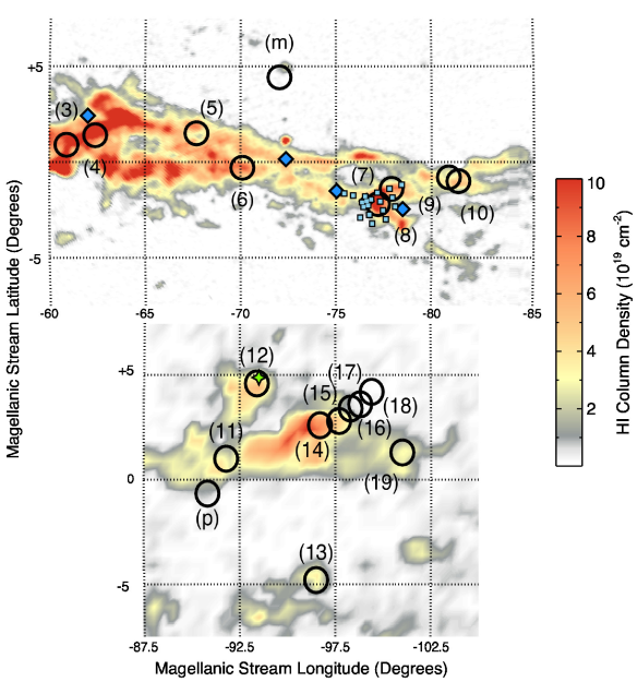
Figure 19: The H i column density map shows the neutral gas distribution from $-60\arcdeg\leq l_{\rm MS}\leq-85\arcdeg$ (Top) and from $-87.5\fdg 5\leq l_{\rm MS}\leq-105\arcdeg$ (Bottom) over $-7\fdg 5\leq b_{\rm MS}\leq+7\fdg 5$. The map and spectra labels coincide with the ones used in Figure 1 and Table 1. The black circles in the H i map represent the positions and coverage area of pointed WHAM observations. The top map displays the H i column density over the range $-375\leq{{\rm v}_{\rm{LSR}}}\leq-175~{}{\rm km\thinspace s^{-1}}$ with H i from GASS H i Survey. The locations of WW96 observations are shown as dark blue diamonds and the positions of the WVW02 and W03 observations are mark with light blue squares. The bottom map over the range $-250\leq{{\rm v}_{\rm{LSR}}}\leq-75~{}{\rm km\thinspace s^{-1}}$ with H i from the LAB H i Survey and the green star marks the location of an PBV03 observation.

Our observations include three sight line pairs that substantially overlap with each other at only $0\fdg 1$ apart (small compared to the $1\arcdeg$ beam size): (4a & 4b), (5a & 5b), and (7a & 7b). The H i distribution of sight lines pairs is pretty constant, as is the H$\alpha$ distribution for (7a & 7b) for the $\sim 100~{}{\rm km\thinspace s^{-1}}$ that they overlap. Along the (4a & 4b) sight lines, the “a” spectrum is enhanced at ${{\rm v}_{\rm{LSR}}}\approx-180$ and $-75~{}{\rm km\thinspace s^{-1}}$. Although the H$\alpha$ spectrum at position (4a) seems to trace emission from the Magellanic Stream over the $-150\leq{{\rm v}_{\rm{LSR}}}\leq-50~{}{\rm km\thinspace s^{-1}}$ range, the large difference between the H i and H$\alpha$ spectra at $-250\leq{{\rm v}_{\rm{LSR}}}\leq-150~{}{\rm km\thinspace s^{-1}}$ preclude us from confidently identifying this as emission. For this reason, we only report an upper limit of ${\rm I}_{\rm H\alpha}<40~{}{\rm mR}$ for the (4a) sight line.

Sight line (5b) has a similar H$\alpha$ enhancement at ${{\rm v}_{\rm{LSR}}}=-175~{}{\rm km\thinspace s^{-1}}$ compared to its (5a) pair. These sight lines lie $\sim 5\arcdeg$ away and $-45~{}{\rm km\thinspace s^{-1}}$ from the (4a & 4b) pair. Unlike the (4a & 4b) pair, the H$\alpha$ between $-200\leq{{\rm v}_{\rm{LSR}}}\leq-100~{}{\rm km\thinspace s^{-1}}$ overlaps substantially with the H i emission at $-175\leq{{\rm v}_{\rm{LSR}}}\leq-125~{}{\rm km\thinspace s^{-1}}$. Therefore we treat the emission along both of the 5a and 5b sight lines as real with aligned H i emission at ${{\rm v}_{\rm{LSR}}}\approx-156~{}{\rm km\thinspace s^{-1}}$ and misaligned H$\alpha$ emission at ${{\rm v}_{\rm{LSR}}}\approx-139~{}{\rm km\thinspace s^{-1}}$ and ${{\rm v}_{\rm{LSR}}}\approx-173~{}{\rm km\thinspace s^{-1}}$, respectively. This velocity offset in these nearby sight lines suggest that there is small scale variation in the Stream. However, H i and H$\alpha$ match up very well for sight lines (7a & 7b), positioned another $10\arcdeg$ down stream. To confidently probe the small scale variation of this tidal remnant, higher spatial resolution observations are needed.

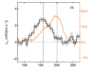
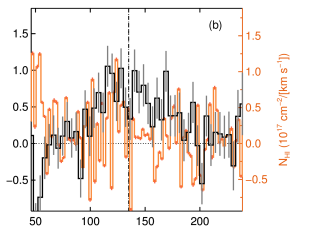
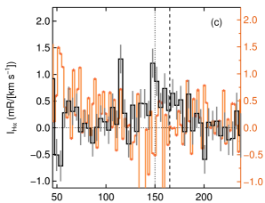
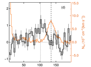
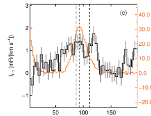
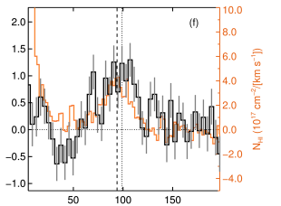
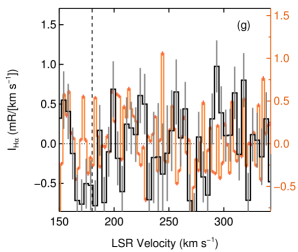
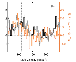
Figure 20: The LAB H i and WHAM H$\alpha$ spectra for all $39$ sight lines, where the letters and numbers coincide with the sight line identifiers listed in Table 1. The vertical dash and dotted lines mark the center of the H i and H$\alpha$ emission, respectively. To reduce small variations in H i column density and the H$\alpha$ intensity, we increased the bin size of the spectra by a factor of two.

References

- Ackermann et al. (2014) Ackermann, M., Albert, A., Atwood, W. B., et al. 2014, ApJ, 793, 64
- Asplund et al. (2009) Asplund, M., Grevesse, N., Sauval, A. J., & Scott, P. 2009, ARA&A, 47, 481
- Barger et al. (2013) Barger, K. A., Haffner, L. M., & Bland-Hawthorn, J. 2013, ApJ, 771, 132
- Barger et al. (2012) Barger, K. A., Haffner, L. M., Wakker, B. P., et al. 2012, ApJ, 761, 145
- Besla et al. (2007) Besla, G., Kallivayalil, N., Hernquist, L., et al. 2007, ApJ, 668, 949
- Besla et al. (2010) —. 2010, ApJ, 721, L97
- Besla et al. (2012) —. 2012, MNRAS, 421, 2109
- Bland-Hawthorn & Cohen (2003) Bland-Hawthorn, J., & Cohen, M. 2003, ApJ, 582, 246
- Bland-Hawthorn & Maloney (1999) Bland-Hawthorn, J., & Maloney, P. R. 1999, ApJ, 510, L33
- Bland-Hawthorn & Maloney (2001) —. 2001, ApJ, 550, L231
- Bland-Hawthorn et al. (2013) Bland-Hawthorn, J., Maloney, P. R., Sutherland, R. S., & Madsen, G. J. 2013, ApJ, 778, 58