The rational SPDE approach for Gaussian random fields with general smoothness

Abstract.

A popular approach for modeling and inference in spatial statistics is to represent Gaussian random fields as solutions to stochastic partial differential equations (SPDEs) of the form $L^{\beta}u=\mathcal{W}$, where $\mathcal{W}$ is Gaussian white noise, $L$ is a second-order differential operator, and $\beta>0$ is a parameter that determines the smoothness of $u$. However, this approach has been limited to the case $2\beta\in\mathbb{N}$, which excludes several important models and makes it necessary to keep $\beta$ fixed during inference.

We propose a new method, the rational SPDE approach, which in spatial dimension $d\in\mathbb{N}$ is applicable for any $\beta>d/4$, and thus remedies the mentioned limitation. The presented scheme combines a finite element discretization with a rational approximation of the function $x^{-\beta}$ to approximate $u$. For the resulting approximation, an explicit rate of convergence to $u$ in mean-square sense is derived. Furthermore, we show that our method has the same computational benefits as in the restricted case $2\beta\in\mathbb{N}$. Several numerical experiments and a statistical application are used to illustrate the accuracy of the method, and to show that it facilitates likelihood-based inference for all model parameters including $\beta$.

1. Introduction

One of the main challenges in spatial statistics is to handle large data sets. A reason for this is that the computational cost for likelihood evaluation and spatial prediction is in general cubic in the number $N$ of observations of a Gaussian random field. A tremendous amount of research has been devoted to coping with this problem and various methods have been suggested (see Heaton et al., 2018, for a recent review).

A common approach is to define an approximation $u_{h}$ of a Gaussian random field $u$ on a spatial domain $\mathcal{D}$ via a basis expansion,

$$u_{h}({\boldsymbol{\mathrm{s}}})=\sum_{j=1}^{n}u_{j}\,\varphi_{j}({\boldsymbol{\mathrm{s}}}),\qquad{\boldsymbol{\mathrm{s}}}\in\mathcal{D},$$ (1.1)

where $\varphi_{j}\colon\mathcal{D}\to\mathbb{R}$ are fixed basis functions and ${\boldsymbol{\mathrm{u}}}=(u_{1},\ldots,u_{n})^{\top}\sim\mathsf{N}({\boldsymbol{\mathrm{0}}},{\boldsymbol{\mathrm{\Sigma}}}_{{\boldsymbol{\mathrm{u}}}})$ are stochastic weights. The computational effort can then be reduced by choosing $n\ll N$. However, methods based on such low-rank approximations tend to remove fine-scale variations of the process. For this reason, methods which instead exploit sparsity for reducing the computational cost have gained popularity in recent years. One can construct sparse approximations either of the covariance matrix of the measurements (Furrer et al., 2006), or of the inverse of the covariance matrix (Datta et al., 2016). Alternatively, one can let the precision matrix ${\boldsymbol{\mathrm{\Sigma}}}_{{\boldsymbol{\mathrm{u}}}}^{-1}$ of the weights in (1.1) be sparse, as in the stochastic partial differential equation (SPDE) approach by Lindgren et al. (2011), where usually $n\approx N$. To increase the accuracy further, several combinations of the methods mentioned above have been considered (e.g., Sang and Huang, 2012) and multiresolution approximations of the process have been exploited (Nychka et al., 2015; Katzfuss, 2017). However, theoretical error bounds have not been derived for most of these methods, which necessitates tuning these approximations for each specific model.

In this work we propose a new class of approximations, whose members we refer to as rational stochastic partial differential equation approximations or rational approximations for short. Our approach is similar to some of the above methods in the sense that an expansion (1.1) with compactly supported basis functions is exploited. The main novelty is that neither the covariance matrix ${\boldsymbol{\mathrm{\Sigma}}}_{{\boldsymbol{\mathrm{u}}}}$ nor the precision matrix ${\boldsymbol{\mathrm{\Sigma}}}_{{\boldsymbol{\mathrm{u}}}}^{-1}$ of the weights ${\boldsymbol{\mathrm{u}}}$ is assumed to be sparse. The covariance matrix is instead a product ${\boldsymbol{\mathrm{\Sigma}}}_{{\boldsymbol{\mathrm{u}}}}={\boldsymbol{\mathrm{P}}}{\boldsymbol{\mathrm{Q}}}^{-1}{\boldsymbol{\mathrm{P}}}^{\top}$, where ${\boldsymbol{\mathrm{P}}}$ and ${\boldsymbol{\mathrm{Q}}}$ are sparse matrices and the sparsity pattern of ${\boldsymbol{\mathrm{P}}}$ is a subset of that of ${\boldsymbol{\mathrm{Q}}}$. We show that the resulting approximation facilitates inference and prediction at the same computational cost as a Markov approximation with ${\boldsymbol{\mathrm{\Sigma}}}_{{\boldsymbol{\mathrm{u}}}}^{-1}={\boldsymbol{\mathrm{Q}}}$, and at a higher accuracy.

For the theoretical framework of our approach, we consider a Gaussian random field on a bounded domain $\mathcal{D}\subset\mathbb{R}^{d}$ which can be represented as the solution $u$ to the SPDE

$$L^{\beta}u=\mathcal{W}\quad\text{in }\mathcal{D},$$ (1.2)

where $\mathcal{W}$ is Gaussian white noise on $\mathcal{D}$, and $L^{\beta}$ is a fractional power of a second-order differential operator $L$ which determines the covariance structure of $u$. Our rational approximations are based on two components: (i) a finite element method (FEM) with continuous and piecewise polynomial basis functions $\{\varphi_{j}\}_{j=1}^{n}$, and (ii) a rational approximation of the function $x^{-\beta}$. We explain how to perform these two steps in practice in order to explicitly compute the matrices ${\boldsymbol{\mathrm{P}}}$ and ${\boldsymbol{\mathrm{Q}}}$. Furthermore, we derive an upper bound for the strong mean-square error of the rational approximation. This bound provides an explicit rate of convergence in terms of the mesh size of the finite element discretization, which facilitates tuning the approximation without empirical tests for each specific model.

Examples of random fields which can be expressed as solutions to SPDEs of the form (1.2) include approximations of Gaussian Matérn fields (Matérn, 1960). Specifically, if $\mathcal{D}:=\mathbb{R}^{d}$ a zero-mean Gaussian Matérn field can be viewed as a solution $u$ to

$$(\kappa^{2}-\Delta)^{\beta}\,(\tau u)=\mathcal{W},$$ (1.3)

where $\Delta$ denotes the Laplacian (Whittle, 1963). The constant parameters $\kappa,\tau>0$ determine the practical correlation range and the variance of $u$. The exponent $\beta$ defines the smoothness parameter $\nu$ of the Matérn covariance function via the relation $2\beta=\nu+d/2$ and, thus, the differentiability of the field. For applications, variance, range and differentiability typically are the most important properties of a Gaussian field. For this reason, the Matérn model is highly popular in spatial statistics and has become the standard choice for Gaussian process priors in machine learning (Rasmussen and Williams, 2006). Since (1.3) is a special case of (1.2) we believe that the outcomes of this work will be of great relevance for many statistical applications, see also §7.

In contrast to covariance-based models, the SPDE approach additionally has the advantage that it allows for a number of generalizations of stationary Matérn fields including (i) non-stationary fields generated by non-stationary differential operators (e.g., Fuglstad et al., 2015), (ii) fields on more general domains such as the sphere (e.g., Lindgren et al., 2011), and (iii) non-Gaussian models (e.g., Wallin and Bolin, 2015).

Lindgren et al. (2011) showed that, if $2\beta\in\mathbb{N}$, one can construct accurate approximations of the form (1.1) for Gaussian Matérn fields on bounded domains $\mathcal{D}\subsetneq\mathbb{R}^{d}$, such that ${\boldsymbol{\mathrm{\Sigma}}}_{{\boldsymbol{\mathrm{u}}}}^{-1}$ is sparse. To this end, (1.3) is considered on $\mathcal{D}$ and the differential operator $\kappa^{2}-\Delta$ is augmented with appropriate boundary conditions. The resulting SPDE is then solved approximately by means of a FEM. Due to the implementation in the R-INLA software, this approach has become widely used, see (Bakka et al., 2018) for a comprehensive list of recent applications.

However, the restriction $2\beta\in\mathbb{N}$ implies a significant limitation for the flexibility of the method. In particular, it is therefore not directly applicable to the important special case of exponential covariance ($\nu=1/2$) on $\mathbb{R}^{2}$, where $\beta=3/4$. In addition, restricting the value of $\beta$ complicates estimating the smoothness of the process from data. In fact, $\beta$ typically is fixed when the method is used in practice, since identifying the value of $2\beta\in\mathbb{N}$ with the highest likelihood requires a separate estimation of all the other parameters in the model for each value of $\beta$. A common justification for fixing $\beta$ is to argue that it is not practicable to estimate the smoothness of a random field from data. However, there are certainly applications for which it is feasible to estimate the smoothness. We provide an example of this in §7. Furthermore, having the correct smoothness of the model is particularly important for interpolation, and the fact that the Matérn model allows for estimating the smoothness from data was the main reason for why Stein (1999) recommended the model.

The rational SPDE approach presented in this work facilitates an estimation of $\beta$ from data by providing an approximation of $u$ which is computable for all fractional powers $\beta>d/4$ (i.e., $\nu>0$), where $d\in\mathbb{N}$ is the dimension of the spatial domain $\mathcal{D}\subset\mathbb{R}^{d}$. It thus enables to include this parameter in likelihood-based (or Bayesian) parameter estimation for both stationary and non-stationary models. Although the SPDE approach has been considered in the non-fractional case also for non-stationary models, Lindgren et al. (2011) showed convergence of the approximation only for the stationary model (1.3). Our analysis in §3 closes this gap since we consider the general model (1.2) which covers the non-stationary case and several other previously proposed generalizations of the Matérn model.

The structure of this article is as follows: We briefly review existing methods for the SPDE approach in the fractional case in §2. In §3 the rational SPDE approximation is introduced and a result on its strong convergence is stated. The procedure of applying the rational SPDE approach to statistical inference is addressed in §4. §5 contains numerical experiments which illustrate the accuracy of the proposed method. The identifiability of the parameters in the Matérn SPDE model (1.3) is discussed in §6, where we derive necessary and sufficient conditions for equivalence of the induced Gaussian measures. In §7 we present an application to climate data, where we consider fractional and non-fractional models for both stationary and non-stationary covariances. We conclude with a discussion in §8. Finally, the supplementary material contains four appendices providing details about (A) the finite element discretization, (B) the convergence analysis, (C) a comparison with the quadrature method by Bolin et al. (2018a), and (D) the equivalence of Gaussian measures. The method developed in this work has been implemented in the R (R Core Team, 2017) package rSPDE (Bolin, 2019).

2. The SPDE approach in the fractional case until now

A reason for why the approach by Lindgren et al. (2011) only works for integer values of $2\beta$ is given by Rozanov (1977), who showed that a Gaussian random field on $\mathbb{R}^{d}$ is Markov if and only if its spectral density can be written as the reciprocal of a polynomial, $\widetilde{S}(\mathbf{k})=(2\pi)^{-d}(\sum_{j=0}^{m}b_{j}\|\mathbf{k}\|^{2j})^{-1}$. Since the spectrum of a Gaussian Matérn field is

$$S(\mathbf{k})=\frac{1}{(2\pi)^{d}}\frac{1}{(\kappa^{2}+\|\mathbf{k}\|^{2})^{2\beta}},\qquad\mathbf{k}\in\mathbb{R}^{d},$$ (2.1)

the precision matrix ${\boldsymbol{\mathrm{Q}}}$ will therefore not be sparse unless $2\beta\in\mathbb{N}$. For $2\beta\notin\mathbb{N}$, Lindgren et al. (2011) suggested to compute a Markov approximation by choosing $m=\lceil 2\beta\rceil$ and selecting the coefficients ${\boldsymbol{\mathrm{b}}}=(b_{1},\ldots,b_{m})^{\top}$ so that the deviation between the spectral densities $\int_{\mathbb{R}^{d}}w(\mathbf{k})(S(\mathbf{k})-\widetilde{S}(\mathbf{k}))^{2}\,\mathrm{d}\mathbf{k}$ is minimized. For this measure of deviation, $w$ is some suitable weight function which should be chosen to get a good approximation of the covariance function. For the method to be useful in practice, the coefficients $b_{j}$ should be given explicitly in terms of the parameters $\kappa$ and $\nu$. Because of this, Lindgren et al. (2011) proposed a weight function that enables an analytical evaluation of the integral,

$$\int_{\kappa^{2}}^{\infty}\Bigl{[}z^{2\beta}-\sum_{j=0}^{m}b_{j}(z-\kappa^{2})^{j}\Bigr{]}^{2}z^{-2m-1-\theta}\,\mathrm{d}z,$$

where $\theta>0$ is a tuning parameter. By differentiating this integral with respect to the parameters and setting the differentials equal to zero, a system of linear equations is obtained, which can be solved to find the coefficients ${\boldsymbol{\mathrm{b}}}$. The resulting approximation depends strongly on $\theta$, and one could use numerical optimization to find a good value of $\theta$ for a specific value of $\beta$, or use the choice $\theta=2\beta-\lfloor 2\beta\rfloor$, which approximately minimizes the maximal distance between the covariance functions (Lindgren et al., 2011). This method was used for the comparison in (Heaton et al., 2018), and we will use it as a baseline method when analyzing the accuracy of the rational SPDE approximations in later sections.

Another Markov approximation based on the spectral density was proposed by Roininen et al. (2018). These Markov approximations may be sufficient in certain applications; however, any approach based on the spectral density or the covariance function is difficult to generalize to models on more general domains than $\mathbb{R}^{d}$, non-stationary models, or non-Gaussian models. Thus, such methods cannot be used if the full potential of the SPDE approach should be kept for fractional values of $\beta$.

There is a rich literature on methods for solving deterministic fractional PDEs (e.g., Bonito and Pasciak, 2015; Gavrilyuk et al., 2004; Jin et al., 2015; Nochetto et al., 2015), and some of the methods that have been proposed could be used to compute approximations of the solution to the SPDE (1.3). However, any deterministic problem becomes more sophisticated when randomness is included. Even methods developed specifically for sampling solutions to SPDEs like (1.3) may be difficult to use directly for statistical applications, when likelihood evaluations, spatial predictions or posterior sampling are needed. For instance, it has been unclear if the sampling approach by Bolin et al. (2018a), which is based on a quadrature approximation for an integral representation of the fractional inverse $L^{-\beta}$, could be used for statistical inference. In Appendix C we show that it can be viewed as a (computationally less efficient) version of the rational SPDE approximations developed in this work. Consequently, the results in §4 on how to use the rational SPDE approach for inference apply also to that method. In §5.1 we compare the performance of the two methods in practice within the scope of a numerical experiment.

3. Rational approximations for fractional SPDEs

In this section we propose an explicit scheme for approximating solutions to a class of SPDEs including (1.3). Specifically, in §3.1–§3.2 we introduce the fractional order equation of interest as well as its finite element discretization. In §3.3 we propose a non-fractional equation, whose solution after specification of certain coefficients approximates the random field of interest. For this approximation, we provide a rigorous error bound in §3.4. Finally, in §3.5 we address the computation of the coefficients in the rational approximation.

3.1. The fractional order equation

With the objective of allowing for more general Gaussian random fields than the Matérn class, we consider the fractional order equation (1.2), where $\mathcal{D}\subset\mathbb{R}^{d}$, $d\in\{1,2,3\}$, is an open, bounded, convex polytope, with closure $\overline{\mathcal{D}}$, and $\mathcal{W}$ is Gaussian white noise in $L_{2}(\mathcal{D})$. Here and below, $L_{2}(\mathcal{D})$ is the Lebesgue space of square-integrable real-valued functions, which is equipped with the inner product $(w,v)_{L_{2}(\mathcal{D})}:=\int_{\mathcal{D}}w({\boldsymbol{\mathrm{s}}})v({\boldsymbol{\mathrm{s}}})\,\mathrm{d}{\boldsymbol{\mathrm{s}}}$. The Sobolev space of order $k\in\mathbb{N}$ is denoted by $H^{k}(\mathcal{D}):=\left\{w\in L_{2}(\mathcal{D}):D^{\gamma}w\in L_{2}(\mathcal{D})\ \forall\,|\gamma|\leq k\right\}$ and $H^{1}_{0}(\mathcal{D})$ is the subspace of $H^{1}(\mathcal{D})$ containing functions with vanishing trace.

We assume that the operator $L\colon\mathscr{D}(L)\subset L_{2}(\mathcal{D})\to L_{2}(\mathcal{D})$ is a linear second-order differential operator in divergence form,

$$Lu=-\nabla\cdot({\boldsymbol{\mathrm{H}}}\nabla u)+\kappa^{2}u,$$ (3.1)

whose domain of definition $\mathscr{D}(L)$ depends on the choice of boundary conditions on $\partial\mathcal{D}$. Specifically, we impose homogeneous Dirichlet or Neumann boundary conditions and set $V=H^{1}_{0}(\mathcal{D})$ or $V=H^{1}(\mathcal{D})$, respectively. Furthermore, we let the functions ${\boldsymbol{\mathrm{H}}}$ and $\kappa$ in (3.1) satisfy the following assumptions:

1. ${\boldsymbol{\mathrm{H}}}\colon\overline{\mathcal{D}}\to\mathbb{R}^{d\times d}$ is symmetric, Lipschitz continuous on the closure $\overline{\mathcal{D}}$, i.e.,

   $$\exists C_{\operatorname{Lip}}>0:\quad|H_{ij}({\boldsymbol{\mathrm{s}}})-H_{ij}({\boldsymbol{\mathrm{s^{\prime}}}})|\leq C_{\operatorname{Lip}}\|{\boldsymbol{\mathrm{s}}}-{\boldsymbol{\mathrm{s^{\prime}}}}\|\qquad\forall{\boldsymbol{\mathrm{s}}},{\boldsymbol{\mathrm{s^{\prime}}}}\in\overline{\mathcal{D}},\quad\forall i,j\in\{1,\ldots,d\},$$

   and uniformly positive definite, i.e.,

   $$\exists C_{0}>0:\quad\operatorname{ess}\inf_{{\boldsymbol{\mathrm{s}}}\in\mathcal{D}}\boldsymbol{\xi}^{\top}{\boldsymbol{\mathrm{H}}}({\boldsymbol{\mathrm{s}}})\boldsymbol{\xi}\geq C_{0}\|\boldsymbol{\xi}\|^{2}\qquad\forall\boldsymbol{\xi}\in\mathbb{R}^{d};$$

2. $\kappa\colon\mathcal{D}\to\mathbb{R}$ is essentially bounded, $\kappa\in L_{\infty}(\mathcal{D})$. Furthermore, if Neumann boundary conditions are imposed, then $\operatorname{ess}\inf_{{\boldsymbol{\mathrm{s}}}\in\mathcal{D}}\kappa({\boldsymbol{\mathrm{s}}})\geq\kappa_{0}>0$ holds.

If I.–II. are satisfied, the differential operator $L$ in (3.1) induces a symmetric, continuous and coercive bilinear form $a_{L}$ on $V$,

$$a_{L}\colon V\times V\to\mathbb{R},\qquad a_{L}(u,v):=({\boldsymbol{\mathrm{H}}}\nabla u,\nabla v)_{L_{2}(\mathcal{D})}+(\kappa^{2}u,v)_{L_{2}(\mathcal{D})},$$ (3.2)

and its domain is given by $\mathscr{D}(L)=H^{2}(\mathcal{D})\cap V$. Furthermore, Weyl’s law (see, e.g., Davies, 1995, Thm. 6.3.1) shows that the eigenvalues $\{\lambda_{j}\}_{j\in\mathbb{N}}$ of the elliptic differential operator $L$ in (3.1), in nondecreasing order, satisfy the spectral asymptotics

$$\lambda_{j}\eqsim j^{2/d}\qquad\text{as }j\to\infty.$$ (3.3)

Thus, existence and uniqueness of the solution $u$ to (1.2) readily follow from Lemma 2.1 and Proposition 2.3 of Bolin et al. (2018a). We formulate this as a proposition.

Proposition 3.1.

Let $L$ be given by (3.1) where ${\boldsymbol{\mathrm{H}}}$ and $\kappa$ satisfy the assumptions I.–II. above and assume $\beta>d/4$. Then (1.2) has a unique solution $u$ in $L_{2}(\Omega;L_{2}(\mathcal{D}))$.

The assumptions I.–II. on the differential operator $L$ are satisfied, e.g., by the Matérn operator $L=\kappa^{2}-\Delta$, in which case the condition $\beta>d/4$ on the fractional exponent in (1.2) corresponds to a positive smoothness parameter $\nu$, i.e., to a non-degenerate field. Moreover, the equation (1.2) as considered in our work includes several previously proposed non-fractional non-stationary models as special cases, such as the non-stationary Matérn models by Lindgren et al. (2011), the models with locally varying anisotropy by Fuglstad et al. (2015), and the barrier models by Bakka et al. (2019). Thus, Proposition 3.1 shows existence and uniqueness of the fractional versions of all these models, which can be treated in practice by using the results of the following sections.

3.2. The discrete model

In order to discretize the problem, we assume that $V_{h}\subset V$ is a finite element space with continuous piecewise linear basis functions $\{\varphi_{j}\}_{j=1}^{n_{h}}$ defined with respect to a triangulation $\mathcal{T}_{h}$ of the domain $\overline{\mathcal{D}}$ indexed by the mesh width $h:=\max_{T\in\mathcal{T}_{h}}h_{T}$, where $h_{T}:=\operatorname{diam}(T)$ is the diameter of the element $T\in\mathcal{T}_{h}$. Furthermore, the family $(\mathcal{T}_{h})_{h\in(0,1)}$ of triangulations inducing the finite-dimensional subspaces $(V_{h})_{h\in(0,1)}$ of $V$ is supposed to be quasi-uniform, i.e., there exist constants $C_{1},C_{2}>0$ such that $\rho_{T}\geq C_{1}h_{T}$ and $h_{T}\geq C_{2}h$ for all $T\in\mathcal{T}_{h}$ and $h\in(0,1)$. Here, $\rho_{T}>0$ is radius of largest ball inscribed in $T\in\mathcal{T}_{h}$.

The discrete operator $L_{h}\colon V_{h}\to V_{h}$ is defined in terms of the bilinear form $a_{L}$ in (3.2) via the relation $(L_{h}\phi_{h},\psi_{h})_{L_{2}(\mathcal{D})}=a_{L}(\phi_{h},\psi_{h})$ which holds for all $\phi_{h},\psi_{h}\in V_{h}$. We then consider the following SPDE on the finite-dimensional state space $V_{h}$,

$$L_{h}^{\beta}u_{h}=\mathcal{W}_{h}\quad\text{in }\mathcal{D},$$ (3.4)

where $\mathcal{W}_{h}$ is Gaussian white noise in $V_{h}$, i.e., $\mathcal{W}_{h}=\sum_{j=1}^{n_{h}}\xi_{j}e_{j,h}$ for a basis $\{e_{j,h}\}_{j=1}^{n_{h}}$ of $V_{h}$ which is orthonormal in $L_{2}(\mathcal{D})$ and $\xi_{j}\sim\mathsf{N}(0,1)$ i.i.d. for $j=1,\ldots,n_{h}$.

We note that the assumptions I.–II. from §3.1 on the functions ${\boldsymbol{\mathrm{H}}}$ and $\kappa$ combined with the convexity of $\mathcal{D}$ imply that the operator $L$ in (3.1) is $H^{2}(\mathcal{D})$-regular, i.e., if $f\in L_{2}(\mathcal{D})$, then the weak solution $u\in V$ to $Lu=f$ satisfies $u\in H^{2}(\mathcal{D})\cap V$, see, e.g., (Grisvard, 2011, Thm. 3.2.1.2) for the case of Dirichlet boundary conditions. By combining this observation with the spectral asymptotics (3.3) we see that the assumptions in Lemmata 3.1 and 3.2 of Bolin et al. (2018a) are satisfied (since then, in their notation, $r=s=q=2$ and $\alpha=2/d$) and we obtain an error estimate for the finite element approximation $u_{h}=L_{h}^{-\beta}\mathcal{W}_{h}$ in (3.4) for all $\beta\in(d/4,1)$. Furthermore, since their derivation requires only that $\beta>d/4$, we can formulate this result for all such values of $\beta$ in the following proposition.

Proposition 3.2.

Suppose that $\beta>d/4$ and that $L$ is given by (3.1) where ${\boldsymbol{\mathrm{H}}}$ and $\kappa$ satisfy the assumptions I.–II. from §3.1. Let $u$, $u_{h}$ be the solutions to (1.2) and (3.4), respectively. Then, there exists a constant $C>0$ such that, for sufficiently small $h$,

$${\color[rgb]{0,0,0}\|u-u_{h}\|_{L_{2}(\Omega;L_{2}(\mathcal{D}))}\leq Ch^{\min\{2\beta-d/2,\,2\}}.}$$

3.3. The rational approximation

Proposition 3.2 shows that the mean-square error between $u$ and $u_{h}$ in $L_{2}(\mathcal{D})$ converges to zero as $h\to 0$. It remains to describe how an approximation of the random field $u_{h}$ with values in the finite-dimensional state space $V_{h}$ can be constructed.

For $\beta\in\mathbb{N}$ one can use, e.g., the iterated finite element method presented in Appendix A to compute $u_{h}$ in (3.4) directly. In the following, we construct approximations of $u_{h}$ if $\beta\not\in\mathbb{N}$ is a fractional exponent. For this purpose, we aim at finding a non-fractional equation

$$P_{\ell,h}u_{h,m}^{R}=P_{r,h}\mathcal{W}_{h}\quad\text{in }\mathcal{D},$$ (3.5)

such that $u_{h,m}^{R}$ is a good approximation of $u_{h}$, and where the operator $P_{j,h}:=p_{j}(L_{h})$ is defined in terms of a polynomial $p_{j}$ of degree $m_{j}\in\mathbb{N}_{0}$, for $j\in\{\ell,r\}$. Since the so-defined operators $P_{\ell,h}$, $P_{r,h}$ commute, this will lead to a nested SPDE model of the form

$$\begin{split}P_{\ell,h}x_{h,m}&=\mathcal{W}_{h}\hskip 32.72049pt\text{in }\mathcal{D},\\ u^{R}_{h,m}&=P_{r,h}x_{h,m}\quad\text{in }\mathcal{D},\end{split}$$ (3.6)

which facilitates efficient computations, see §4 and Appendix A.

Comparing the initial equation (1.2) with

$$P_{\ell}u_{m}^{R}=P_{r}\mathcal{W}\quad\text{in }\mathcal{D},$$ (3.7)

where $P_{j}:=p_{j}(L)$, $j\in\{\ell,r\}$, motivates the choice $m_{\ell}-m_{r}\approx\beta$ in order to obtain a similar smoothness of $u_{m}^{R}=(P_{r}^{-1}P_{\ell})^{-1}\mathcal{W}$ and $u=L^{-\beta}\mathcal{W}$ in (1.2). In practice, we first choose a degree $m\in\mathbb{N}$ and then set

$$m_{r}:=m\qquad\text{and}\qquad m_{\ell}:=m+m_{\beta},\qquad\text{where}\qquad m_{\beta}:=\max\{1,\lfloor\beta\rfloor\}.$$ (3.8)

In this case, the solution $u_{m}^{R}$ of (3.7) has the same smoothness as the solution $v$ of the non-fractional equation $L^{\lfloor\beta\rfloor}v=\mathcal{W}$, if $\beta\geq 1$, and as $v$ in $Lv=\mathcal{W}$, if $\beta<1$. Note that, for fixed $h$, the degree $m$ controls the accuracy of the approximation $u_{h,m}^{R}$.

We now turn to the problem of defining the non-fractional operators $P_{\ell,h}$ and $P_{r,h}$ in (3.5). In order to compute $u_{h}$ in (3.4) directly, one would have to apply the discrete fractional inverse $L_{h}^{-\beta}$ to the noise term $\mathcal{W}_{h}$ on the right-hand side. Therefore, a first idea would be to approximate the function $x^{-\beta}$ on the spectrum of $L_{h}$ by a rational function $\widetilde{r}$ and to use $\widetilde{r}(L_{h})\mathcal{W}_{h}$ as an approximation of $u_{h}$. This is, in essence, the approach proposed by Harizanov et al. (2018) to find optimal solvers for the problem ${\boldsymbol{\mathrm{L}}}^{\beta}{\boldsymbol{\mathrm{x}}}={\boldsymbol{\mathrm{f}}}$, where ${\boldsymbol{\mathrm{L}}}$ is a sparse symmetric positive definite matrix. However, the spectra of $L$ and of $L_{h}$ as $h\to 0$ (considered as operators on $L_{2}(\mathcal{D})$) are unbounded and, thus, it would be necessary to normalize the spectrum of $L_{h}$ for every $h$, since it is not feasible to construct the rational approximation $\widetilde{r}$ on an unbounded interval. We aim at an approximation $L_{h}^{-\beta}\approx p_{\ell}(L_{h})^{-1}p_{r}(L_{h})$, where in practice the choice of $p_{\ell}$ and $p_{r}$ can be made independent of $L_{h}$ and $h$. Thus, we pursue another idea.

In contrast to the differential operator $L$ in (3.1), its inverse $L^{-1}\colon L_{2}(\mathcal{D})\to L_{2}(\mathcal{D})$ is compact and, thus, the spectra of $L^{-1}$ and of $L_{h}^{-1}$ are bounded subsets of the intervals $J:=\bigl{[}0,\lambda_{1}^{-1}\bigr{]}$ and $J_{h}:=\bigl{[}\lambda_{n_{h},h}^{-1},\lambda_{1,h}^{-1}\bigr{]}\subset J$, respectively, where $\lambda_{1,h},\lambda_{n_{h},h}>0$ are the smallest and the largest eigenvalue of $L_{h}$. This motivates a rational approximation $r$ of the function $f(x):=x^{\beta}$ on $J$ and to deduce the non-fractional equation (3.5) from $u_{h,m}^{R}=r(L_{h}^{-1})\mathcal{W}_{h}$.

In order to achieve our envisaged choice (3.8) of different polynomial degrees $m_{\ell}$ and $m_{r}$, we decompose $f$ via $f(x)=\hat{f}(x)x^{m_{\beta}}$, where $\hat{f}(x):=x^{\beta-m_{\beta}}$. We approximate $\hat{f}\approx\hat{r}:=\frac{q_{1}}{q_{2}}$ on $J_{h}$, where $q_{1}(x):=\sum_{i=0}^{m}c_{i}x^{i}$ and $q_{2}(x):=\sum_{j=0}^{m+1}b_{j}x^{j}$ are polynomials of degree $m$ and $m+1$, respectively, and use $r(x):=\hat{r}(x)x^{m_{\beta}}$ as an approximation for $f$. This construction leads (after expanding the fraction with $x^{m}$) to a rational approximation $\frac{p_{r}}{p_{\ell}}$ of $x^{-\beta}$,

$$x^{-\beta}=f(x^{-1})\approx\hat{r}(x^{-1})x^{-m_{\beta}}=\frac{q_{1}(x^{-1})}{q_{2}(x^{-1})x^{m_{\beta}}}=\frac{\sum_{i=0}^{m}c_{i}x^{m-i}}{\sum_{j=0}^{m+1}b_{j}x^{m+m_{\beta}-j}},$$ (3.9)

where the polynomials $p_{r}(x):=\sum_{i=0}^{m}c_{i}x^{m-i}$ and $p_{\ell}(x):=\sum_{j=0}^{m+1}b_{j}x^{m+m_{\beta}-j}$ are of degree $m$ and $m+m_{\beta}$, respectively, i.e., (3.8) is satisfied.

The operators $P_{\ell,h}$, $P_{r,h}$ in (3.5) are defined accordingly,

$$P_{\ell,h}:=p_{\ell}(L_{h})=\sum_{j=0}^{m+1}b_{j}L_{h}^{m+m_{\beta}-j},\qquad P_{r,h}:=p_{r}(L_{h})=\sum_{i=0}^{m}c_{i}L_{h}^{m-i}.$$ (3.10)

Their continuous counterparts in (3.7) are $P_{\ell}:=p_{\ell}(L)$ and $P_{r}:=p_{r}(L)$. We note that, for (3.8) to hold, any choice $m_{2}\in\{0,1,\ldots,m+m_{\beta}\}$ would have been permissible for the polynomial degree of $q_{2}$, if $m$ is the degree of $q_{1}$. The reason for setting $m_{2}=m+1$ is that this is the maximal choice which is universally applicable for all values of $\beta>d/4$.

In the following we refer to $u_{h,m}^{R}$ in (3.5) with $P_{\ell,h}$, $P_{r,h}$ defined by (3.10) as the rational SPDE approximation of degree $m$. We emphasize that this approximation relies (besides the finite element discretization) only on the rational approximation of the function $\hat{f}$. In particular, no information about the operator $L$ except for a lower bound of the eigenvalues is needed. In the Matérn case, we have $L=\kappa^{2}-\Delta$ (with certain boundary conditions) and an obvious lower bound of the eigenvalues is therefore given by $\kappa^{2}$.

3.4. An error bound for the rational approximation

In this subsection we justify the approach proposed in §3.2–§3.3 by providing an upper bound for the strong mean-square error $\|u-u_{h,m}^{R}\|_{L_{2}(\Omega;L_{2}(\mathcal{D}))}$. Here $u$ and $u_{h,m}^{R}$ are the solutions of (1.2) and (3.5) and the rational approximation $u_{h,m}^{R}$ is constructed as described in §3.3, assuming that $\hat{r}=\hat{r}_{h}$ is the $L_{\infty}$-best rational approximation of $\hat{f}(x)=x^{\beta-m_{\beta}}$ on the interval $J_{h}$ for each $h$. This means that $\hat{r}_{h}$ minimizes the error in the supremum norm on $J_{h}$ among all rational approximations of the chosen degrees in numerator and denominator. How such approximations can be computed is discussed in §3.5.

The theoretical analysis presented in Appendix B results in the following theorem, showing strong convergence of the rational approximation $u_{h,m}^{R}$ to the exact solution $u$.

Theorem 3.3.

Suppose that $\beta>d/4$ and that $L$ is given by (3.1) where ${\boldsymbol{\mathrm{H}}}$ and $\kappa$ satisfy the assumptions I.–II. from §3.1. Let $u$, $u_{h,m}^{R}$ be the solutions to (1.2) and (3.5), respectively. Then, there is a constant $C>0$, independent of $h,m$, such that, for sufficiently small $h$,

$${\color[rgb]{0,0,0}\|u-u_{h,m}^{R}\|_{L_{2}(\Omega;L_{2}(\mathcal{D}))}\leq C\Bigl{(}h^{\min\{2\beta-d/2,\,2\}}+\mathbbm{1}_{\beta\notin\mathbb{N}}h^{\min\{2(\beta-1),\,0\}-d/2}e^{-2\pi\sqrt{|\beta-m_{\beta}|m}}\Bigr{)}.}$$

Remark 3.4.

In order to calibrate the accuracy of the rational approximation with the finite element error, one can choose $m\in\mathbb{N}$ such that $e^{-2\pi\sqrt{|\beta-m_{\beta}|m}}\propto h^{2\max\{\beta,\,1\}}$. The strong rate of mean-square convergence is then $\min\{2\beta-d/2,\,2\}$.

Remark 3.5.

If the functions ${\boldsymbol{\mathrm{H}}}$ and $\kappa$ of the operator $L$ in (3.1) are smooth, ${\boldsymbol{\mathrm{H}}}\in C^{\infty}(\overline{\mathcal{D}})^{d\times d}$ and $\kappa\in C^{\infty}(\overline{\mathcal{D}})$ (as, e.g., in the Matérn case) and if the domain $\mathcal{D}$ has a smooth boundary, the higher-order strong mean-square convergence rate $\min\{2\beta-d/2,\,p+1\}$ can be proven for a finite element method with continuous basis functions which are piecewise polynomial of degree at most $p\in\mathbb{N}$. Thus, for $\beta>1$, finite elements with $p>1$ may be meaningful.

3.5. Computing the coefficients of the rational approximation

As explained in §3.3, the coefficients $\{c_{i}\}_{i=0}^{m}$ and $\{b_{j}\}_{j=0}^{m+1}$ needed for defining the operators $P_{\ell,h}$, $P_{r,h}$ in (3.10) are obtained from a rational approximation $\hat{r}=\hat{r}_{h}$ of $\hat{f}(x)=x^{\beta-m_{\beta}}$ on $J_{h}$. For each $h$, this approximation can, e.g., be computed with the second Remez algorithm (Remez, 1934), which generates the coefficients of the $L_{\infty}$-best approximation. The error analysis for the resulting approximation $u_{h,m}^{R}$ in (3.5) was performed in §3.4. Despite the theoretical benefit of generating the $L_{\infty}$-best approximation, the Remez algorithm is often unstable in computations and, therefore, we use a different method in our simulations. However, versions of the Remez scheme were used, e.g., by Harizanov et al. (2018).

A simpler and computationally more stable way of choosing the rational approximation is, for instance, the Clenshaw–Lord Chebyshev–Padé algorithm (Baker and Graves-Morris, 1996). To further improve the stability of the method, we will rescale the operator $L$ so that its eigenvalues are bounded from below by one, which for the Matérn case corresponds to reformulating the SPDE (1.3) as $(\mathrm{Id}-\kappa^{-2}\Delta)^{\beta}(\widetilde{\tau}u)=\mathcal{W}$ and using $L=\mathrm{Id}-\kappa^{-2}\Delta$, where $\mathrm{Id}$ denotes the identity on $L_{2}(\mathcal{D})$ and $\widetilde{\tau}:=\kappa^{2\beta}\tau$.

In order to avoid computing a different rational approximation $\hat{r}$ for each finite element mesh width $h$, in practice we compute the approximation $\hat{r}$ only once on the interval $J_{*}:=[\delta,1]$, where $\delta\in(0,1)$ should ideally be chosen such that $J_{h}\subset J_{*}$ for all considered mesh sizes $h$. For the numerical experiments later, we will use $\delta=10^{-(5+m)/2}$ when computing rational approximations of order $m$, which gives acceptable results for all values of $\beta$. As an example, the coefficients computed with the Clenshaw–Lord Chebyshev–Padé algorithm on $J_{*}$ for the case of exponential covariance on $\mathbb{R}^{2}$ are shown in Table 1.

$m$	$b_{0}$	$c_{0}$	$b_{1}$	$c_{1}$	$b_{2}$	$c_{2}$	$b_{3}$	$c_{3}$	$b_{4}$
1	1.69e-2	7.69e-2	8.06e-1	1	2.57e-1
2	8.08e-4	5.30e-3	1.98e-1	4.05e-1	1.07	1	1.41e-1
3	3.72e-5	3.27e-4	3.03e-2	8.57e-2	6.84e-1	1.00	1.28	1	9.17e-2

Table 1. Coefficients of the rational approximation for $\beta=3/4$ (exponential covariance on $\mathbb{R}^{2}$) for $m=1,2,3$, normalized so that $c_{m}=1$.

4. Computational aspects of the rational approximation

In the non-fractional case, the sparsity of the precision matrix for the weights ${\boldsymbol{\mathrm{u}}}$ in (1.1) facilitates fast computation of samples, likelihoods, and other quantities of interest for statistical inference. The purpose of this section is to show that the rational SPDE approximation proposed in §3 preserves these good computational properties.

The representation (3.6) shows that $u_{h,m}^{R}$ can be seen as a Markov random field $x_{h,m}$, transformed by the operator $P_{r,h}$. Solving this latent model as explained in Appendix A, yields an approximation of the form (1.1), where ${\boldsymbol{\mathrm{\Sigma}}}_{{\boldsymbol{\mathrm{u}}}}=\mathbf{P}_{r}{\boldsymbol{\mathrm{Q}}}^{-1}\mathbf{P}_{r}^{\top}$. Here $\mathbf{P}_{\ell},\mathbf{P}_{r}\in\leavevmode\nobreak\ \mathbb{R}^{n_{h}\times n_{h}}$ correspond to the discrete operators $P_{\ell,h}$ and $P_{r,h}$ in (3.10), respectively. The matrix ${\boldsymbol{\mathrm{Q}}}:=\mathbf{P}_{\ell}^{\top}{\boldsymbol{\mathrm{C}}}^{-1}\mathbf{P}_{\ell}$ is sparse if the mass matrix ${\boldsymbol{\mathrm{C}}}$ with respect to the finite element basis $\{\varphi_{j}\}_{j=1}^{n_{h}}$ is replaced by the diagonal lumped mass matrix $\widetilde{{\boldsymbol{\mathrm{C}}}}$, see Appendix A. By defining ${\boldsymbol{\mathrm{x}}}\sim\mathsf{N}({\boldsymbol{\mathrm{0}}},{\boldsymbol{\mathrm{Q}}}^{-1})$, we have ${\boldsymbol{\mathrm{u}}}=\mathbf{P}_{r}{\boldsymbol{\mathrm{x}}}$, which is a transformed Gaussian Markov random field (GMRF). Choosing ${\boldsymbol{\mathrm{x}}}$ as a latent variable instead of ${\boldsymbol{\mathrm{u}}}$ thus enables us to use all computational methods, which are available for GMRFs (see Rue and Held, 2005), also for the rational SPDE approximation.

As an illustration, we consider the following hierarchical model, with a latent field $u$ which is a rational approximation of (1.2),

$$\begin{split}y_{i}&=u(\mathbf{s}_{i})+\varepsilon_{i},\quad i=1,\ldots,N,\\ P_{\ell}u&=P_{r}\mathcal{W}\qquad\quad\,\,\,\text{in }\mathcal{D},\end{split}$$ (4.1)

where $u$ is observed under i.i.d. Gaussian measurement noise $\varepsilon_{i}\sim\mathsf{N}(0,\sigma^{2})$. Given that one can treat this case, one can easily adapt the method to be used for inference in combination with MCMC or INLA (Rue et al., 2009) for models with more sophisticated likelihoods.

Defining the matrix ${\boldsymbol{\mathrm{A}}}$ with elements $A_{ij}=\varphi_{j}(\mathbf{s}_{i})$ and the vector ${\boldsymbol{\mathrm{y}}}=(y_{1},\ldots,y_{N})^{\top}$ gives us the discretized model

$$\begin{split}{\boldsymbol{\mathrm{y}}}|{\boldsymbol{\mathrm{x}}}&\sim\mathsf{N}({\boldsymbol{\mathrm{A}}}\mathbf{P}_{r}{\boldsymbol{\mathrm{x}}},\sigma^{2}{\boldsymbol{\mathrm{I}}}),\\ {\boldsymbol{\mathrm{x}}}&\sim\mathsf{N}({\boldsymbol{\mathrm{0}}},{\boldsymbol{\mathrm{Q}}}^{-1}).\end{split}$$ (4.2)

In this way, the problem has been reduced to a standard latent GMRF model and a sparse Cholesky factorization of ${\boldsymbol{\mathrm{Q}}}$ can be used for sampling ${\boldsymbol{\mathrm{x}}}$ from $\mathsf{N}({\boldsymbol{\mathrm{0}}},{\boldsymbol{\mathrm{Q}}}^{-1})$ as well as to evaluate its log-density $\log\pi_{x}({\boldsymbol{\mathrm{x}}})$. Samples of ${\boldsymbol{\mathrm{u}}}$ can then be obtained from samples of ${\boldsymbol{\mathrm{x}}}$ via ${\boldsymbol{\mathrm{u}}}=\mathbf{P}_{r}{\boldsymbol{\mathrm{x}}}$. For evaluating the log-density of ${\boldsymbol{\mathrm{u}}}$, $\log\pi_{u}({\boldsymbol{\mathrm{u}}})$, the relation $\log\pi_{u}({\boldsymbol{\mathrm{u}}})=\log\pi_{x}(\mathbf{P}_{r}^{-1}{\boldsymbol{\mathrm{u}}})$ can be exploited. Furthermore, the posterior distribution of ${\boldsymbol{\mathrm{x}}}$ is given by ${\boldsymbol{\mathrm{x}}}|{\boldsymbol{\mathrm{y}}}\sim\mathsf{N}\bigl{(}{\boldsymbol{\mathrm{\mu}}}_{{\boldsymbol{\mathrm{x}}}|{\boldsymbol{\mathrm{y}}}},{\boldsymbol{\mathrm{Q}}}_{{\boldsymbol{\mathrm{x}}}|{\boldsymbol{\mathrm{y}}}}^{-1}\bigr{)}$, where ${\boldsymbol{\mathrm{\mu}}}_{{\boldsymbol{\mathrm{x}}}|{\boldsymbol{\mathrm{y}}}}=\sigma^{-2}{\boldsymbol{\mathrm{Q}}}_{{\boldsymbol{\mathrm{x}}}|{\boldsymbol{\mathrm{y}}}}^{-1}\mathbf{P}_{r}^{\top}{\boldsymbol{\mathrm{A}}}^{\top}{\boldsymbol{\mathrm{y}}}$ and ${\boldsymbol{\mathrm{Q}}}_{{\boldsymbol{\mathrm{x}}}|{\boldsymbol{\mathrm{y}}}}={\boldsymbol{\mathrm{Q}}}+\sigma^{-2}\mathbf{P}_{r}^{\top}{\boldsymbol{\mathrm{A}}}^{\top}{\boldsymbol{\mathrm{A}}}\mathbf{P}_{r}$ is a sparse matrix. Thus, simulations from the distribution of ${\boldsymbol{\mathrm{x}}}|{\boldsymbol{\mathrm{y}}}$, and evaluations of the corresponding log-density $\log\pi_{x|y}({\boldsymbol{\mathrm{x}}})$, can be performed efficiently via a sparse Cholesky factorization of ${\boldsymbol{\mathrm{Q}}}_{{\boldsymbol{\mathrm{x}}}|{\boldsymbol{\mathrm{y}}}}$. Finally, the marginal data log-likelihood is proportional to

$$\log|\mathbf{P}_{\ell}|-\frac{1}{2}\log|{\boldsymbol{\mathrm{Q}}}_{{\boldsymbol{\mathrm{x}}}|{\boldsymbol{\mathrm{y}}}}|-N\log\sigma-\frac{1}{2}\left({\boldsymbol{\mathrm{\mu}}}_{{\boldsymbol{\mathrm{x}}}|{\boldsymbol{\mathrm{y}}}}^{\top}{\boldsymbol{\mathrm{Q}}}\,{\boldsymbol{\mathrm{\mu}}}_{{\boldsymbol{\mathrm{x}}}|{\boldsymbol{\mathrm{y}}}}+\sigma^{-2}\left\|{\boldsymbol{\mathrm{y}}}-{\boldsymbol{\mathrm{A}}}\mathbf{P}_{r}{\boldsymbol{\mathrm{\mu}}}_{{\boldsymbol{\mathrm{x}}}|{\boldsymbol{\mathrm{y}}}}\right\|^{2}\right).$$

We therefore conclude that all computations needed for statistical inference can be facilitated by sparse Cholesky factorizations of $\mathbf{P}_{\ell}$ and ${\boldsymbol{\mathrm{Q}}}_{{\boldsymbol{\mathrm{x}}}|{\boldsymbol{\mathrm{y}}}}$.

Remark 4.1.

From the specific form of the matrices $\mathbf{P}_{\ell}$ and $\mathbf{P}_{r}$ addressed in Appendix A, we can infer that the number of non-zero elements in ${\boldsymbol{\mathrm{Q}}}_{{\boldsymbol{\mathrm{x}}}|{\boldsymbol{\mathrm{y}}}}$ for a rational SPDE approximation of degree $m$ will be the same as the number of non-zero elements in ${\boldsymbol{\mathrm{Q}}}_{{\boldsymbol{\mathrm{x}}}|{\boldsymbol{\mathrm{y}}}}$ for the standard (non-fractional) SPDE approach with $\beta=m+m_{\beta}$. Thus, also the computational cost will be comparable for these two cases.

Remark 4.2.

The matrix ${\boldsymbol{\mathrm{Q}}}_{{\boldsymbol{\mathrm{x}}}|{\boldsymbol{\mathrm{y}}}}$ can be ill-conditioned for $m>1$ if a FEM approximation with piecewise linear basis functions is used. The numerical stability for large values of $m$ can likely be improved by increasing the polynomial degree of the FEM basis functions, see also Remark 3.5.

5. Numerical experiments

5.1. The Matérn covariance on $\mathbb{R}^{2}$

As a first test, we investigate the performance of the rational SPDE approach for Gaussian Matérn fields, without including the finite element discretization in space.

The spectral density $S$ of the solution to (1.3) on $\mathbb{R}^{2}$ is given by (2.1), whereas the spectral density for the non-discretized rational SPDE approximation $u_{m}^{R}$ in (3.7) is

$$S_{R}({\boldsymbol{\mathrm{k}}})\propto\kappa^{4\beta}\left(\frac{\sum_{i=1}^{m}c_{i}(1+\kappa^{-2}\|{\boldsymbol{\mathrm{k}}}\|^{2})^{m-i}}{\sum_{j=1}^{m+1}b_{j}(1+\kappa^{-2}\|{\boldsymbol{\mathrm{k}}}\|^{2})^{m+m_{\beta}-j}}\right)^{2}.$$ (5.1)

We compute the coefficients as described in §3.5. To this end, we apply an implementation of the Clenshaw–Lord Chebyshev–Padé algorithm provided by the Matlab package Chebfun (Driscoll et al., 2014). By performing a partial fraction decomposition of (5.1), expanding the square, transforming to polar coordinates, and using the equality

$$\int_{0}^{\infty}\frac{\omega J_{0}(\omega h)}{(\omega^{2}+a^{2})(\omega^{2}+b^{2})}\,\mathrm{d}\omega=\frac{1}{(b^{2}-a^{2})}(K_{0}(ah)-K_{0}(bh)),$$

we are able to compute the corresponding covariance function $C_{R}(h)$ analytically. Here, $J_{0}$ is a Bessel function of the first kind and $K_{0}$ is a modified Bessel function of the second kind. To measure the accuracy of the approximation, we compare $C_{R}(h)$ to the true Matérn covariance function $C(h)$ for different values of $\nu$, where $\kappa=\sqrt{8\nu}$ is chosen such that the practical correlation range $r=\sqrt{8\nu}/\kappa$ equals one in all cases.

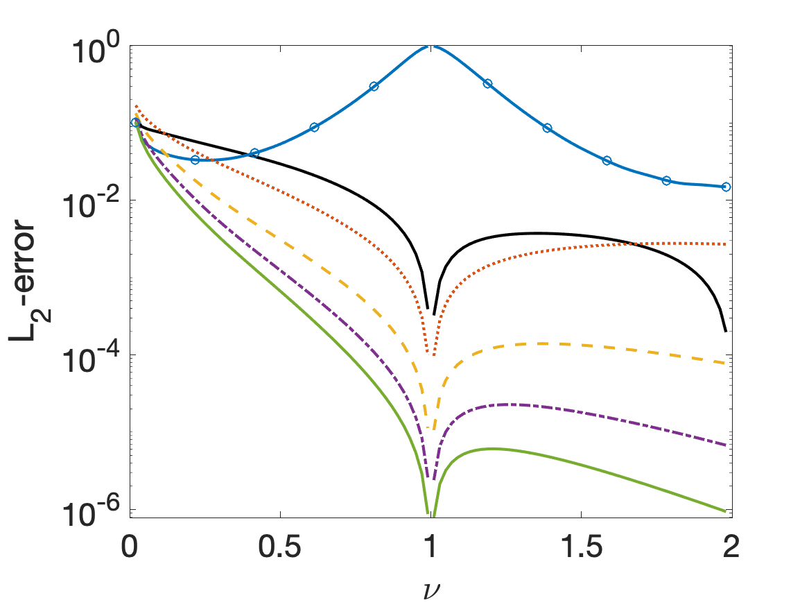
Figure 1. The $L_{2}$- and $L_{\infty}$-errors of the covariance functions for different values of $\nu$ for the different approximation methods. When $\nu=1$, all methods are exact.

To put the accuracy of the rational approximation in context, the Markov approximation by Lindgren et al. (2011) and the quadrature method by Bolin et al. (2018a) are also shown. For the quadrature method, $K=12$ quadrature nodes are used, which results in an approximation with the same computational cost as a rational approximation of degree $m=11$, see Appendix C. Figure 1 shows the normalized error in the $L_{2}$-norm and the error with respect to $L_{\infty}$-norm for different values of $\nu$, both with respect to the interval $[0,2]$ of length twice the practical correlation range, i.e.,

$$\left(\frac{\int_{0}^{2}(C(h)-C_{a}(h))^{2}\,\mathrm{d}h}{\int_{0}^{2}C(h)^{2}\,\mathrm{d}h}\right)^{1/2}\quad\text{and}\quad\sup_{h\in[0,2]}|C(h)-C_{a}(h)|.$$

Here, $C_{a}$ is the covariance function obtained by the respective approximation method.

Already for $m=3$, the rational approximation performs better than both the Markov approximation and the quadrature approximation for all values of $\nu$. It also decreases the error for the case of an exponential covariance by several orders of magnitude.

All methods are exact when $\nu=1$, since this is the non-fractional case. The Markov and rational methods show errors decreasing to zero as $\nu=1$, whereas the error of the quadrature method has a singularity at $\nu=1$. The performance of the quadrature method can be improved (although not the behavior near $\nu=1$) by increasing the number of quadrature nodes, see Appendix C. This is reasonable if the method is needed only for sampling from the model, but implementing this method for statistical applications, which require kriging or likelihood evaluations, is not feasible since the computational costs then are comparable to the standard SPDE approach with $\beta=K$.

Finally, it should be noted that the Markov method also is exact at $\nu=2$ ($\beta=1.5$) since the spectrum of the process then is the reciprocal of a polynomial. The rational and quadrature methods cannot exploit this fact, since these approximations are based on the corresponding differential operator instead of the spectral density. This is the prize that has to be paid in order to formulate a method which works not only for the stationary Matérn fields but also for non-stationary and non-Gaussian models.

5.2. Computational cost and the finite element error

From the study in the previous subsection, we infer that the rational SPDE approach performs well for Matérn fields with arbitrary smoothness. However, as for the standard SPDE approach, we need to discretize the problem in order to be able to use the method in practice, e.g., for inference. This induces an additional error source, which means that one should balance the two errors by choosing the degree $m$ of the rational approximation appropriately with respect to the FEM error. A calibration based on the theoretical results has been suggested in Remark 3.4. In this section we address this issue in practice and investigate the computational cost of the rational SPDE approximation.

As a test case, we compute approximations of a Gaussian Matérn field with unit variance and practical correlation range $r=0.1$ on the unit square in $\mathbb{R}^{2}$. We assume homogeneous Neumann boundary conditions for the Matérn operator $\kappa^{2}-\Delta$ in (1.3). For the discretization, we use a FEM with a nodal basis of continuous piecewise linear functions with respect to a mesh induced by a Delaunay triangulation of a regular lattice on the domain, with a total of $n_{h}$ nodes. We consider three different meshes with $n_{h}=57^{2},85^{2},115^{2}$, which corresponds to $h\approx r/4,r/6,r/8$.

In order to measure the accuracy, we compute the covariances between the midpoint of the domain $\tilde{{\boldsymbol{\mathrm{s}}}}_{*}$ and all other nodes in the lattice $\{\tilde{{\boldsymbol{\mathrm{s}}}}_{j}\}_{j=1}^{n_{h}}$ for the Matérn field and the rational SPDE approximations and calculate the error similarly to the $L_{2}$-error in §5.1,

$$\left(\frac{\sum_{j=1}^{n_{h}}(C(\|\tilde{{\boldsymbol{\mathrm{s}}}}_{*}-\tilde{{\boldsymbol{\mathrm{s}}}}_{j}\|)-\Sigma^{{\boldsymbol{\mathrm{u}}}}_{j,*})^{2}}{\sum_{j=1}^{n_{h}}C(\|\tilde{{\boldsymbol{\mathrm{s}}}}_{*}-\tilde{{\boldsymbol{\mathrm{s}}}}_{j}\|)^{2}}\right)^{1/2},$$

where ${\boldsymbol{\mathrm{\Sigma}}}^{{\boldsymbol{\mathrm{u}}}}=\mathbf{P}_{r}\mathbf{P}_{\ell}^{-1}{\boldsymbol{\mathrm{C}}}\mathbf{P}_{\ell}^{-\top}\mathbf{P}_{r}^{\top}$ is the covariance matrix of ${\boldsymbol{\mathrm{u}}}$, see Appendix A. As a consequence of imposing boundary conditions, the error of the covariance is larger close to the boundary of the domain. However, we compare this error to the error of the non-fractional SPDE approach, which has the same boundary effects. As measures of the computational cost, we consider the time it takes to sample ${\boldsymbol{\mathrm{u}}}$ and to evaluate $\log|{\boldsymbol{\mathrm{Q}}}_{{\boldsymbol{\mathrm{x}}}|{\boldsymbol{\mathrm{y}}}}|$ for the model (4.2) with $\sigma=1$, when ${\boldsymbol{\mathrm{y}}}$ is a vector of noisy observations of the latent field at $1000$ locations, drawn at random in the domain (a similar computation time is needed to evaluate ${\boldsymbol{\mathrm{\mu}}}_{{\boldsymbol{\mathrm{x}}}|{\boldsymbol{\mathrm{y}}}}$).

		Rational SPDE approximation			Standard SPDE approach
$n$		$m=1$	$m=2$	$m=3$	$\beta=2$	$\beta=3$	$\beta=4$
$57^{2}$	Error	1.849	1.339	1.415	2.259	2.173	2.147
	Time	1.5 (3.2)	1.8 (5.2)	2.7 (8.7)	1.7 (2.6)	1.7 (3.9)	2.2 (6.3)
$85^{2}$	Error	1.720	0.757	0.807	0.953	0.928	0.921
	Time	3.1 (8.4)	5.0 (14)	7.6 (25)	3.0 (8.2)	5.8 (13)	7.9 (22)
$115^{2}$	Error	1.559	0.526	0.501	0.509	0.498	0.494
	Time	7.6 (22)	11 (34)	18 (57)	6.3 (18)	11 (35)	18 (53)

Table 2. Covariance errors ($\times 100$) and computing times in seconds ($\times 100$) for sampling from the rational SPDE approximation ${\boldsymbol{\mathrm{u}}}$ (with $\beta=3/4$) and, in parentheses, for evaluating $\log|{\boldsymbol{\mathrm{Q}}}_{{\boldsymbol{\mathrm{x}}}|{\boldsymbol{\mathrm{y}}}}|$. These values are also given for the standard SPDE approach with $\beta=2,3,4$.

The results for rational SPDE approximations of different degrees for the case $\beta=3/4$ (exponential covariance) are shown in Table 2. Furthermore, we perform the same experiment when the standard (non-fractional) SPDE approach is used for $\beta=2,3,4$. As previously mentioned in Remark 4.1, the computational cost of the rational SPDE approximation of degree $m$ should be comparable to the standard SPDE approach with $\beta=m+1$. Table 2 validates this claim. One can also note that the errors of the rational SPDE approximations are similar to those of the standard SPDE approach, and that the reduction in error when increasing from $m=2$ to $m=3$ is small for all cases, indicating that the error induced by the rational approximation is small compared to the FEM error, even for a low degree $m$. This is also the reason for why, in particular in the pre-asymptotic region, one can in practice choose the degree $m$ smaller than the value suggested in Remark 3.4, which gives $m\approx 6,7,8$ for $\beta=3/4$ and the three considered finite element meshes.

6. Likelihood-based inference of Matérn parameters

The computationally efficient evaluation of the likelihood of the rational SPDE approximation facilitates likelihood-based inference for all parameters of the Matérn model, including $\nu$ which until now had to be fixed when using the SPDE approach. In this section we first discuss the identifiability of the model parameters and then investigate the accuracy of this approach within the scope of a simulation study.

6.1. Parameter identifiability

A common reason for fixing the smoothness in Gaussian Matérn models is the result by Zhang (2004) which shows that all three Matérn parameters cannot be estimated consistently under infill asymptotics. More precisely, for a fixed smoothness parameter $\nu$, one cannot estimate both the variance of the field, $\phi^{2}$, and the scale parameter, $\kappa$, consistently. However, the quantity $\phi^{2}\kappa^{2\nu}$ can be estimated consistently. The derivation of this result relies on the equivalence of Gaussian measures corresponding to Matérn fields (Zhang, 2004, Theorem 2). The following theorem provides the analogous result for the Gaussian measures induced by the class of random fields specified via (1.3) on a bounded domain. Its proof can be found in Appendix D.

Theorem 6.1.

Let $\mathcal{D}\subset\mathbb{R}^{d}$, $d\in\{1,2,3\}$, be bounded, open and connected. For $i\in\{1,2\}$, let $\beta_{i}>d/4$, $\kappa_{i},\tau_{i}>0$, and consider the centered Gaussian measure $\mu_{i}:=\mathsf{N}(0,\mathcal{Q}_{i}^{-1})$ on $L_{2}(\mathcal{D})$ with precision operator $\mathcal{Q}_{i}:=\tau_{i}^{2}L_{i}^{2\beta_{i}}$, where the operators $L_{i}:=\kappa_{i}^{2}-\Delta$, $i\in\{1,2\}$, are augmented with the same homogeneous Neumann or Dirichlet boundary conditions. Then, $\mu_{1}$ and $\mu_{2}$ are equivalent if and only if $\beta_{1}=\beta_{2}$ and $\tau_{1}=\tau_{2}$.

Note that, for $\mathcal{D}:=\mathbb{R}^{d}$, the parameter $\tau$ is related to the variance of the Gaussian random field via $\phi^{2}=\Gamma(\nu)(\tau^{2}\Gamma(2\beta)(4\pi)^{d/2}\kappa^{2\nu})^{-1}$. Thus, $\tau^{-2}\propto\phi^{2}\kappa^{2\nu}$, which means that Theorem 6.1 is in accordance with the result by Zhang (2004). Since the Gaussian measures induced by the operators $L_{1}=\tau(\kappa_{1}+\Delta)^{\beta}$ and $L_{2}=\tau(\kappa_{2}+\Delta)^{\beta}$ are equivalent, we will not be able to consistently estimate $\kappa$ under infill asymptotics. Yet, Theorem 6.1 suggests that it is possible to estimate $\tau$ and $\beta$ consistently. In fact, with Theorem 6.1 available, it is straightforward to show that $\tau$ can be estimated consistently for a fixed $\nu$ by exploiting the same arguments as in the proof of (Zhang, 2004, Theorem 3). However, it is beyond the scope of this article to show that both $\nu$ and $\tau$ can be estimated consistently which would also extend the results by Zhang (2004).

6.2. Simulation study

To numerically investigate the accuracy of likelihood-based parameter estimation using the rational SPDE approach, we again assume homogeneous Neumann boundary conditions for the Matérn operator in (1.3) and consider the standard latent model (4.1) from §4. We take the unit square as the domain of interest, set $\sigma^{2}=0.1$, $\nu=0.5$ and choose $\kappa$ and $\tau$ so that the latent field has variance $\phi^{2}=1$ and practical correlation range $r=0.2$. For the FEM, we take a mesh based on a regular lattice on the domain, extended by twice the correlation range in each direction to reduce boundary effects, yielding a mesh with approximately $3500$ nodes.

As a first test case, we use simulated data from the discretized model. We simulate $50$ replicates of the latent field, each with corresponding noisy observations at $1000$ measurement locations drawn at random in the domain. This results in a total of $50000$ observations, which we use to estimate the parameters of the model. We draw initial values for the parameters at random and then numerically optimize the likelihood of the model with the function fminunc in Matlab. This procedure is repeated $100$ times, each time with a new simulated data set.

As a second test case, we repeat the simulation study, but this time we simulate the data from a Gaussian Matérn field with an exponential covariance function instead of from the discretized model. For the estimation, we compute the rational SPDE approximation for the same finite element mesh as in the first test case. To investigate the effect of the mesh resolution on the parameter estimates, we also estimate the parameters using a uniformly refined mesh with twice as many nodes. The average computation time for evaluating the likelihood is approximately $0.16s$ for the coarse mesh and $0.4s$ for the fine mesh. This computation time is affine with respect to the number of replicates, and with only one replicate it is $0.09s$ for the coarse mesh and $0.2s$ for the fine mesh.

		Rational samples	Matérn samples
	Truth	Estimate	Coarse mesh	Fine mesh
$\kappa$	10	10.026 (0.5661)	10.966 (1.8060)	10.864 (0.4414)
$\phi^{2}$	1.0	1.0014 (0.0228)	1.1089 (0.6155)	0.9743 (0.0210)
$\sigma^{2}$	0.1	0.1001 (0.0009)	0.3016 (0.0036)	0.2320 (0.0044)
$\nu$	0.5	0.5011 (0.0168)	0.5554 (0.0991)	0.5462 (0.0138)

Table 3. Results of the parameter estimation. For each parameter estimate, the mean of 100 different estimates is shown, with the corresponding standard deviation in parentheses.

The results of the parameter estimation can be seen in Table 3, where the true parameter values are shown together with the mean and standard deviations of the $100$ estimates for each case. Notably, we are able to estimate all parameters accurately in the first case. For the second case, the finite element discretization seems to induce a small bias, especially for the nugget estimate ($\sigma^{2}$) that depends on the resolution of the mesh. The bias in the nugget estimate is not surprising since the increased nugget compensates for the FEM error. The bias could be decreased by choosing the mesh more carefully, also taking the measurement locations into account. In practice, however, this bias will not be of great importance, since the optimal nugget for the discretized model should be used.

It should be noted that there are several other methods for decreasing the computational cost of likelihood-based inference for stationary Matérn models. The major advantage of the rational SPDE approach is that it is directly applicable to more complicated non-stationary models, which we will use in the next section when analyzing real data.

7. Application

In this section we illustrate for the example of a climate reanalysis data set how the rational SPDE approach can be used for spatial modeling.

Climate reanalysis data is generated by combining a climate model with observations in order to obtain a description of the recent climate. We use reanalysis data generated with the Experimental Climate Prediction Center Regional Spectral Model (ECPC-RSM) which was originally prepared for the North American Regional Climate Change Assessment Program (NARCCAP) by means of NCEP/DOE Reanalysis (Mearns et al., 2014, 2009). As variable we consider average summer precipitation over the conterminous U.S. for a 26 year period from 1979 to 2004. The average value for each grid cell and year is computed as the average of the corresponding daily values for the days in June, July, and August. In order to obtain data which can be modelled by a Gaussian distribution, we follow Genton and Kleiber (2015) and transform the data by taking the cube root. We then subtract the mean over the 26 years from each grid cell so that we can assume that the data has zero mean and focus on the correlation structure of the residuals. The resulting residuals for the year 1979 are shown in Figure 2.

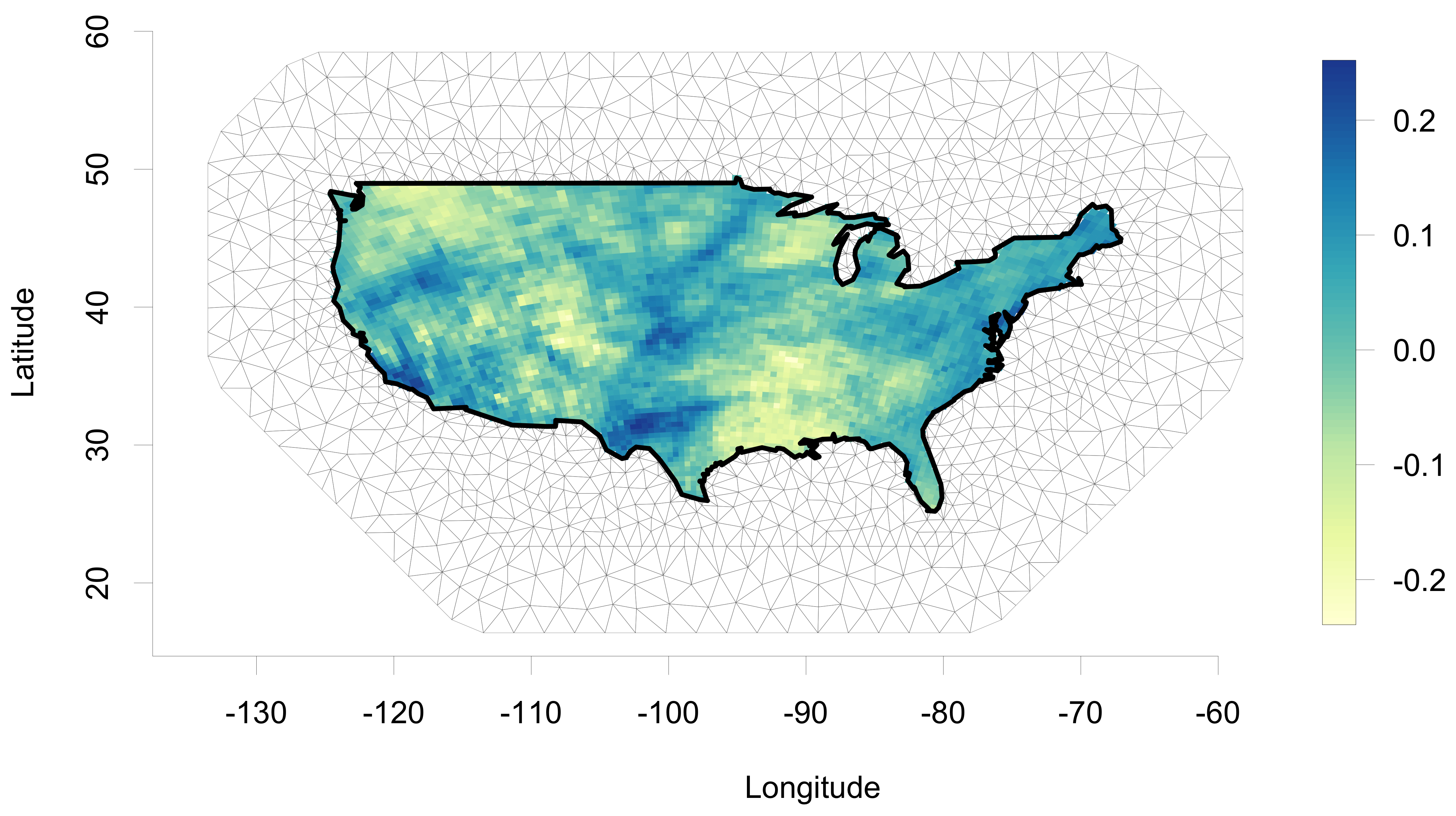
Figure 2. Average summer precipitation residuals (in cm) for 1979 and the FEM mesh.

The 4112 observed residuals for each year are modeled as independent realizations of a zero-mean Gaussian random field with a nugget effect. That is, the measurement $Y_{ij}$ at spatial location ${\boldsymbol{\mathrm{s}}}_{i}$ for year $j$ is modeled as $Y_{ij}=u_{j}({\boldsymbol{\mathrm{s}}}_{i})+\varepsilon_{ij}$, where $\varepsilon_{ij}\sim\mathsf{N}(0,\sigma^{2})$ are independent, and $\{u_{j}({\boldsymbol{\mathrm{s}}})\}_{j}$ are independent realizations of a zero-mean Gaussian random field $u({\boldsymbol{\mathrm{s}}})$. The analysis of Genton and Kleiber (2015) revealed that an exponential covariance model is suitable for a subset of this data set. Because of this, a natural first choice is to use a stationary Matérn model (1.3), either with $\beta=0.75$ (exponential covariance) or with a general $\beta$ which we estimate from the data. However, since we have data for a larger spatial region than Genton and Kleiber (2015), one would suspect that a non-stationary model for $u({\boldsymbol{\mathrm{s}}})$ might be needed. The standard non-stationary model for the SPDE approach, as first suggested by Lindgren et al. (2011) and used in many applications since then, is

$$(\kappa({\boldsymbol{\mathrm{s}}})^{2}-\Delta)^{\beta}\,(\tau({\boldsymbol{\mathrm{s}}})u({\boldsymbol{\mathrm{s}}}))=\mathcal{W}({\boldsymbol{\mathrm{s}}}),\quad{\boldsymbol{\mathrm{s}}}\in\mathcal{D},$$ (7.1)

where $\beta=1$ is fixed. Until now, it has not been possible to use the model (7.1) with fractional smoothness. Therefore, our main question is now: What is more important for this data—the fractional smoothness $\beta$ or the non-stationary parameters? We thus consider four different SPDE models for $u({\boldsymbol{\mathrm{s}}})$. Two of them are non-fractional models, where $\beta=1$ is fixed, and for the other two (fractional) models, we estimate the fractional order $\beta$ jointly with the other parameters from the data. For both cases, we consider stationary Matérn and non-stationary models, where the latter are formulated via (7.1) with

$$\log\kappa({\boldsymbol{\mathrm{s}}})=\kappa_{0}+\kappa_{\rm a}\psi_{\rm a}({\boldsymbol{\mathrm{s}}})+\sum_{i,j=1}^{2}\sum_{k,\ell=1}^{2}\kappa_{ij}^{k\ell}\,\psi_{i}^{k}(\widetilde{s}_{1})\,\psi_{j}^{\ell}(\widetilde{s}_{2}),$$

and the same model is used for $\tau({\boldsymbol{\mathrm{s}}})$. Here, $\psi_{j}^{1}(\widetilde{s}):=\sin(j\pi\widetilde{s})$, $\psi_{j}^{2}(\widetilde{s}):=\cos(j\pi\widetilde{s})$, $\psi_{\rm a}({\boldsymbol{\mathrm{s}}})$ is the altitude at location ${\boldsymbol{\mathrm{s}}}$, and $\widetilde{{\boldsymbol{\mathrm{s}}}}=(\widetilde{s}_{1},\widetilde{s}_{2})$ denotes the spatial coordinate after rescaling so that the observational domain is mapped to the unit square. Thus, $\log\kappa({\boldsymbol{\mathrm{s}}})$ and $\log\tau({\boldsymbol{\mathrm{s}}})$ are modelled by the altitude covariate and 16 additional Fourier basis functions to capture large-scale trends in the parameters. The altitude covariate and the eight Fourier basis functions $\left\{\psi_{1}^{k}(\widetilde{s}_{1})\psi_{j}^{\ell}(\widetilde{s}_{2}):j,k,\ell=1,2\right\}$ are shown in Figure 3.

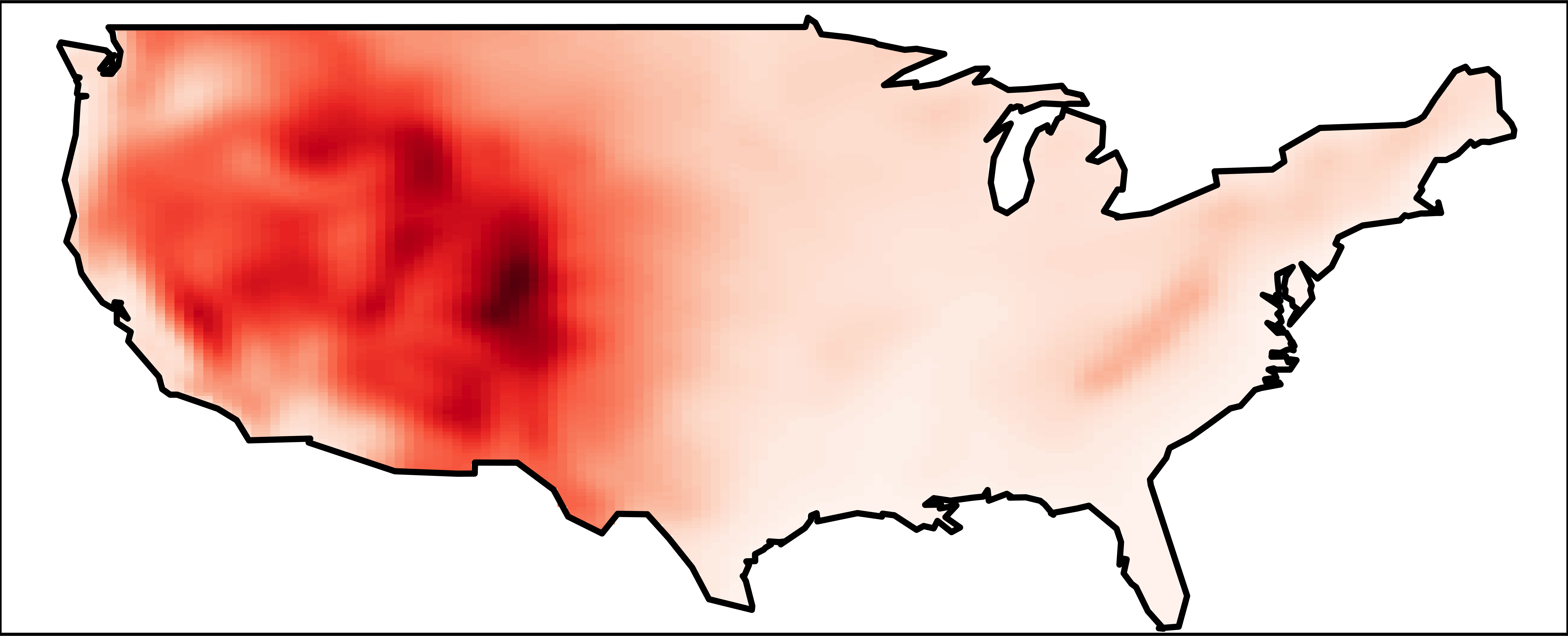
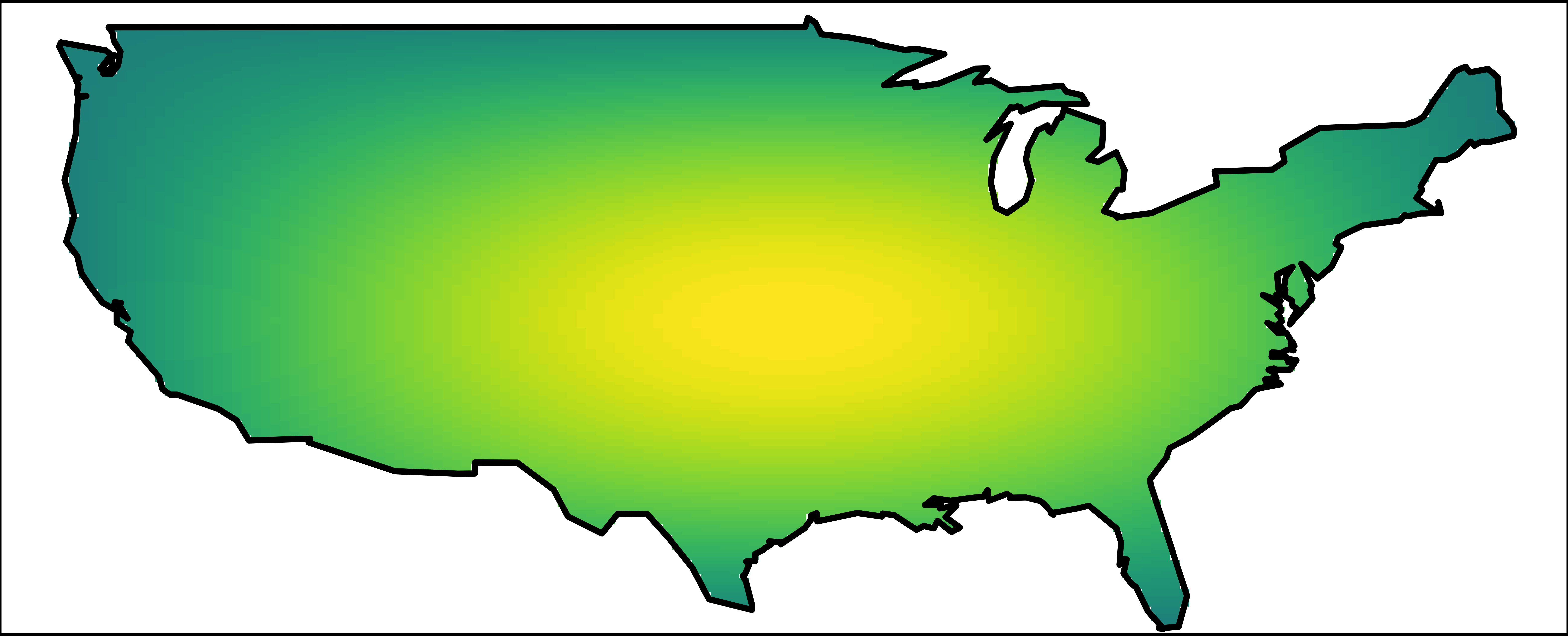
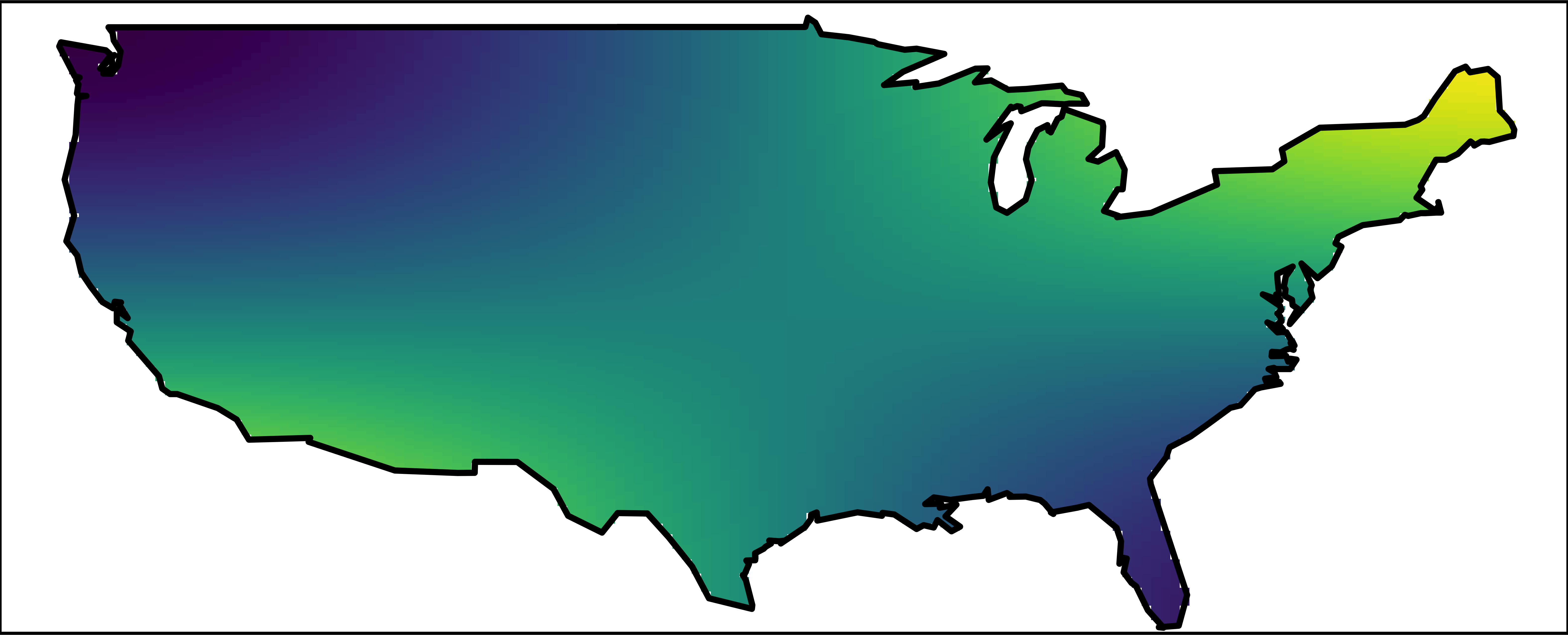
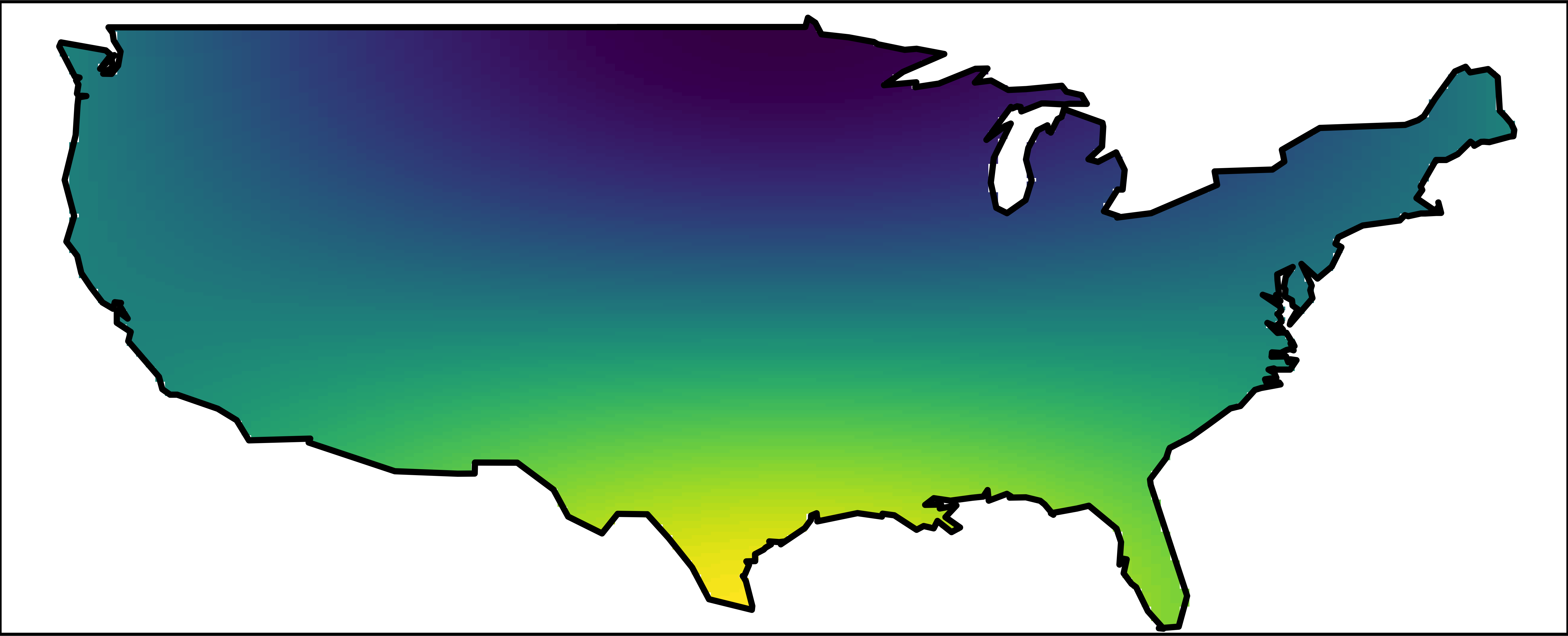
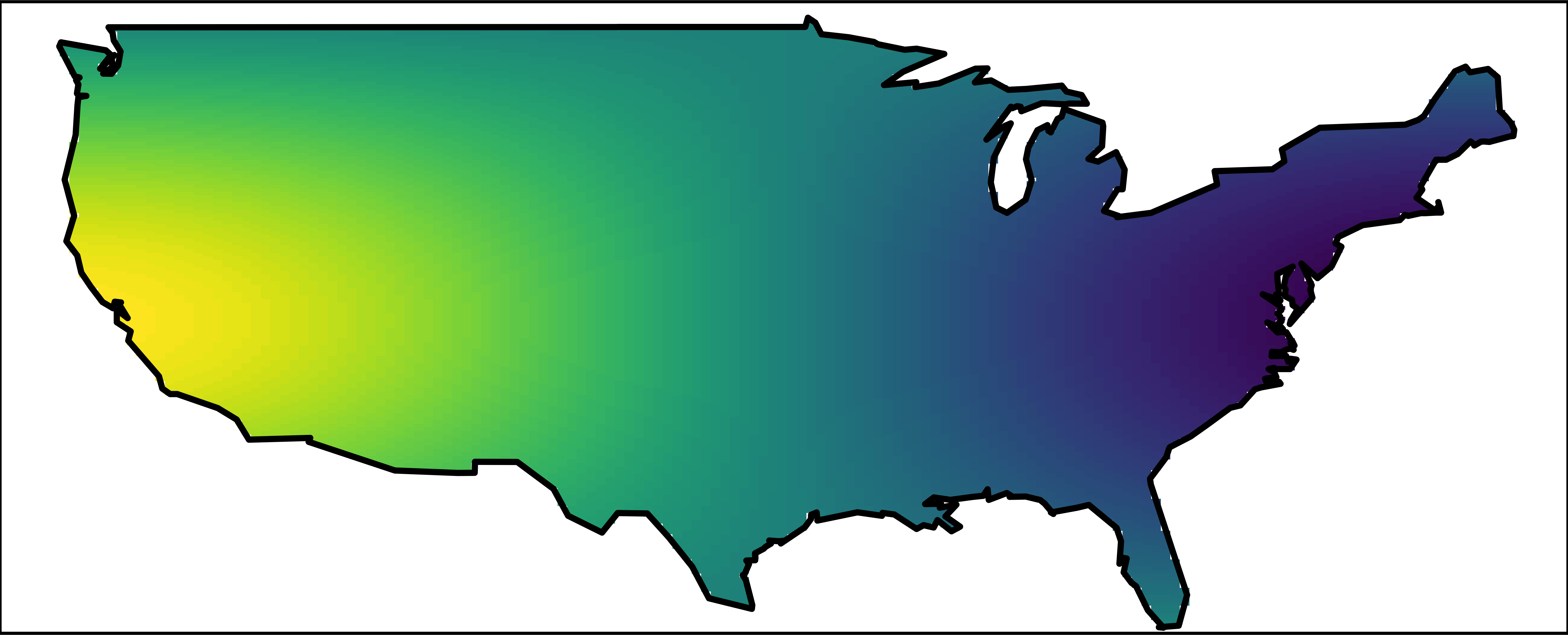
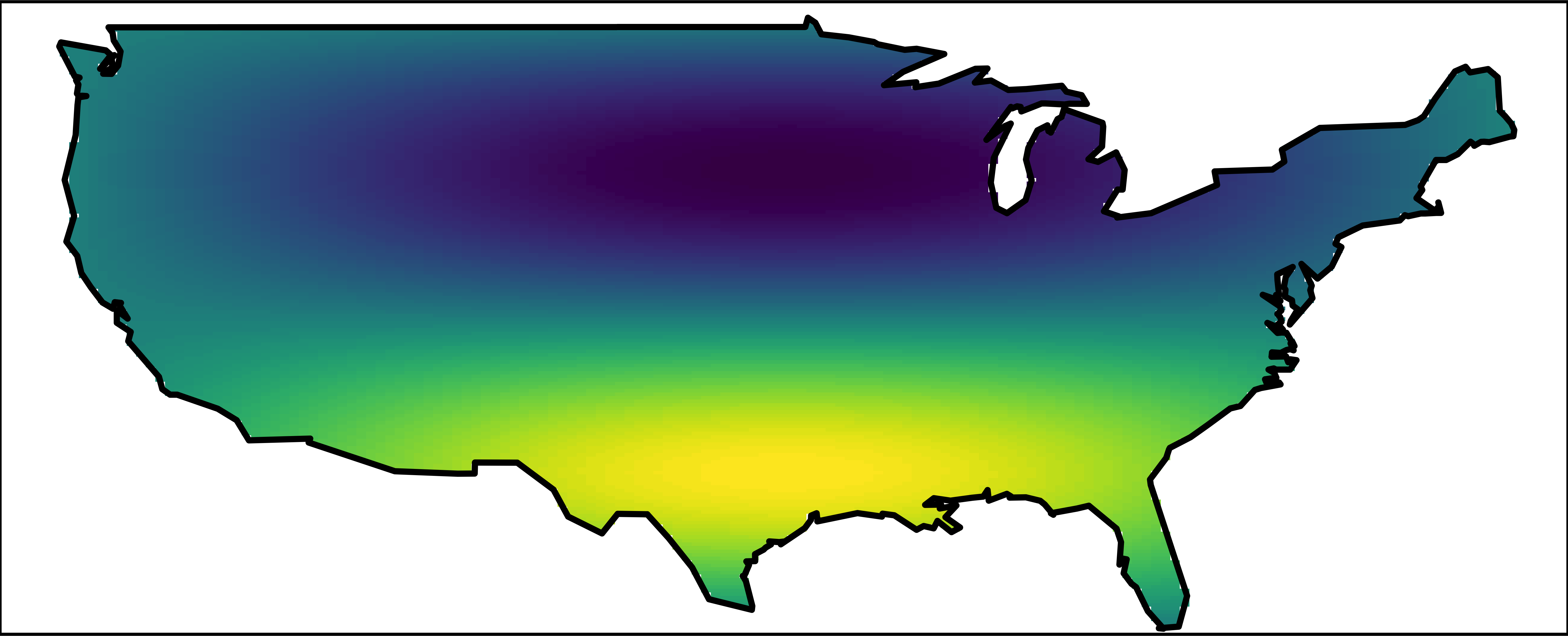
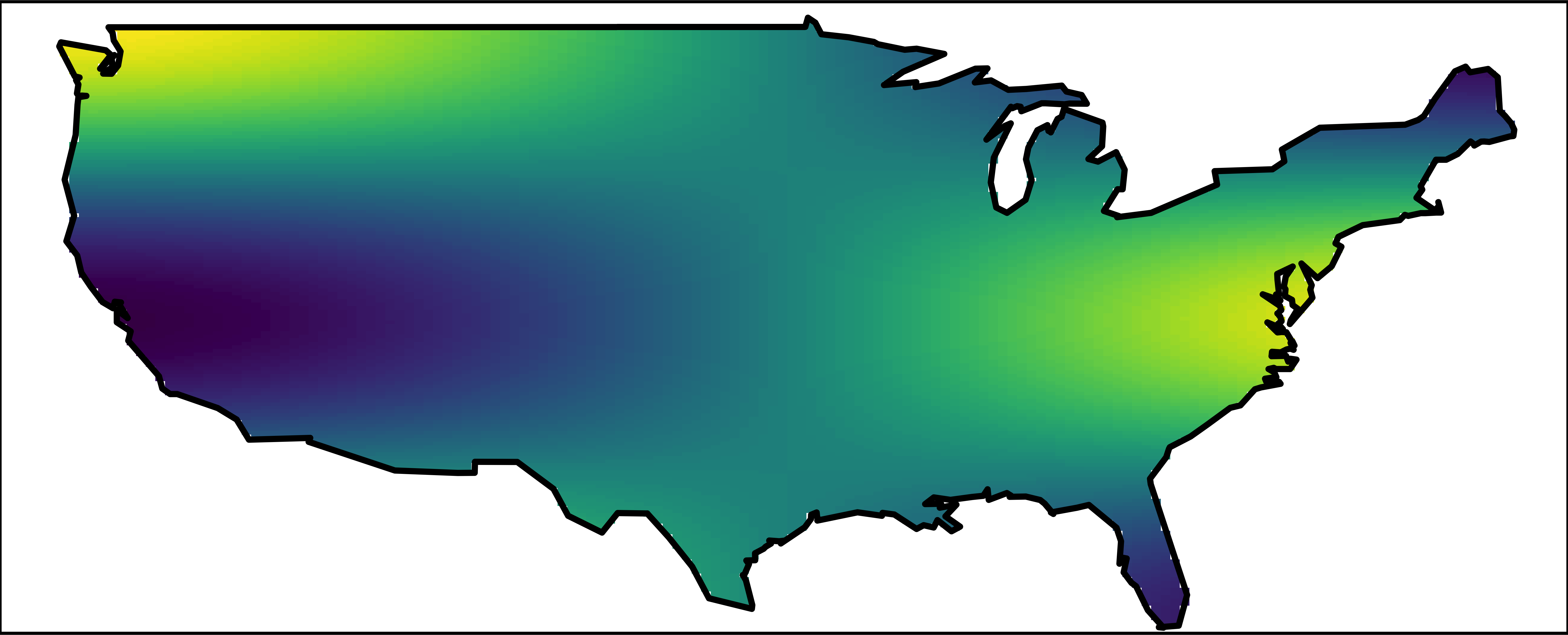
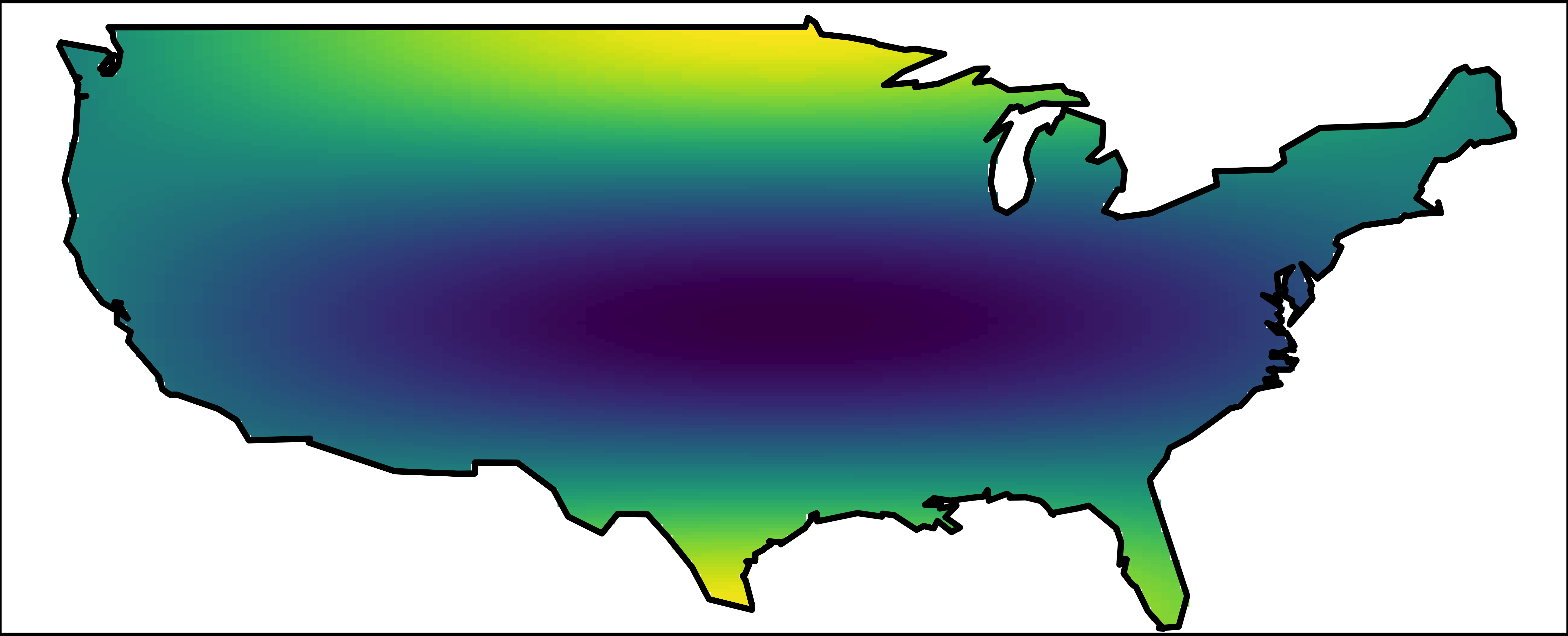
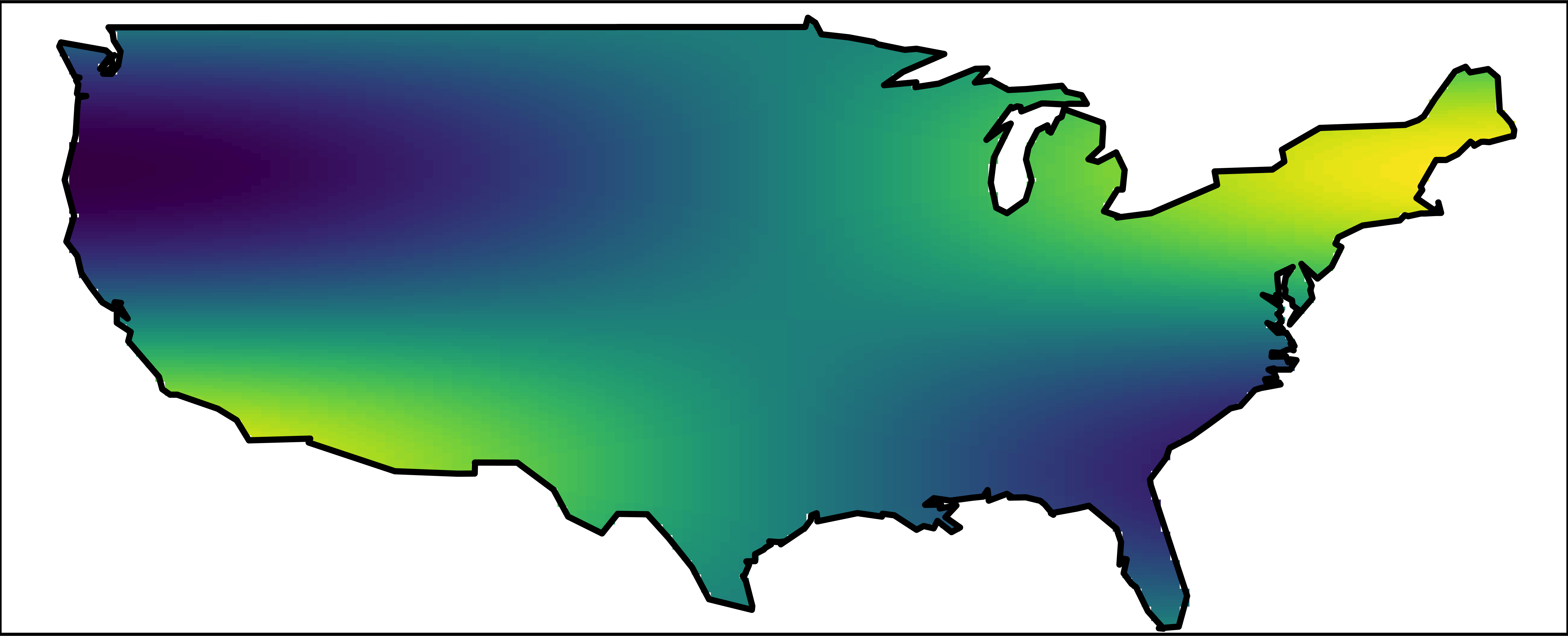
Figure 3. Nine basis functions modeling the parameters for the non-stationary models.

We discretize each model with respect to the finite element mesh shown in Figure 2, assuming homogeneous Neumann boundary conditions. The mesh has $5021$ nodes and was computed using R-INLA (Lindgren and Rue, 2015). For the fractional models, we set $m=1$ in the rational approximation and, for each model, the model parameters are estimated by numerical optimization of the log-likelihood as described in §4.

The log-likelihood values for the four models can be seen in Table 4. The parameter estimates for the stationary non-fractional ($\beta=\nu=1$) model are $\kappa=0.67$, $\tau=5.44$, and $\sigma=0.014$, which implies a standard deviation $\phi=0.077$ and a practical range $\rho=4.21$. The estimates for the fractional model are $\kappa=0.20$, $\tau=10.58$, $\sigma=0.012$, and $\beta=0.72$, corresponding to $\phi=0.081$, $\rho=9.21$, and a smoothness parameter $\nu=0.44$. We note that the fractional model has a longer correlation range. This is likely to be caused by the non-fractional model underestimating the range $\rho$ in order to compensate for the wrong local behavior of the covariance function induced by the smoothness parameter $\nu=1$.

Figure 4 shows the estimated marginal standard deviation $\phi({\boldsymbol{\mathrm{s}}})$ for the two non-stationary models (computed using the estimates of the parameters for $\kappa({\boldsymbol{\mathrm{s}}})$ and $\tau({\boldsymbol{\mathrm{s}}})$) and $0.7$ contours of the correlation function for selected locations in the domain. The estimate of $\beta$ for the non-stationary fractional model is $0.723$. Also for the non-stationary models, we observe a slightly longer practical correlation range $\rho({\boldsymbol{\mathrm{s}}})$ for the fractional model.

Fractional model

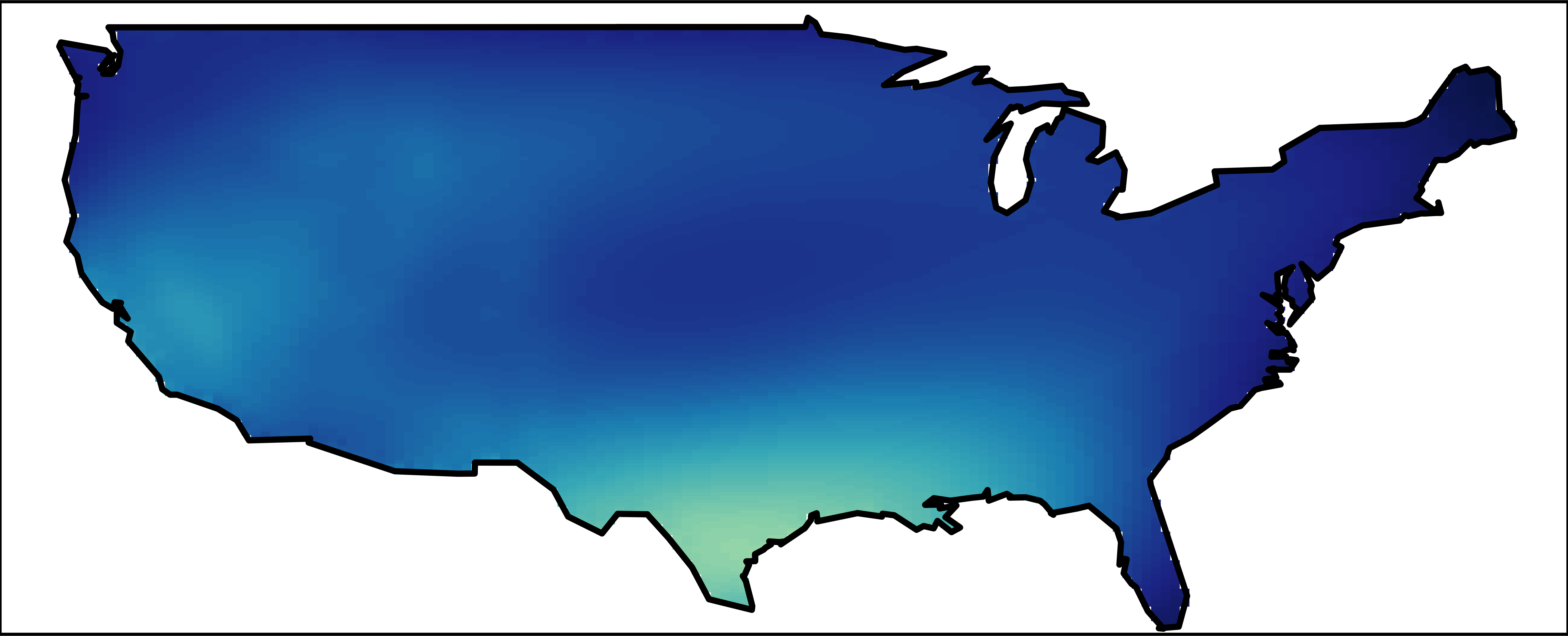
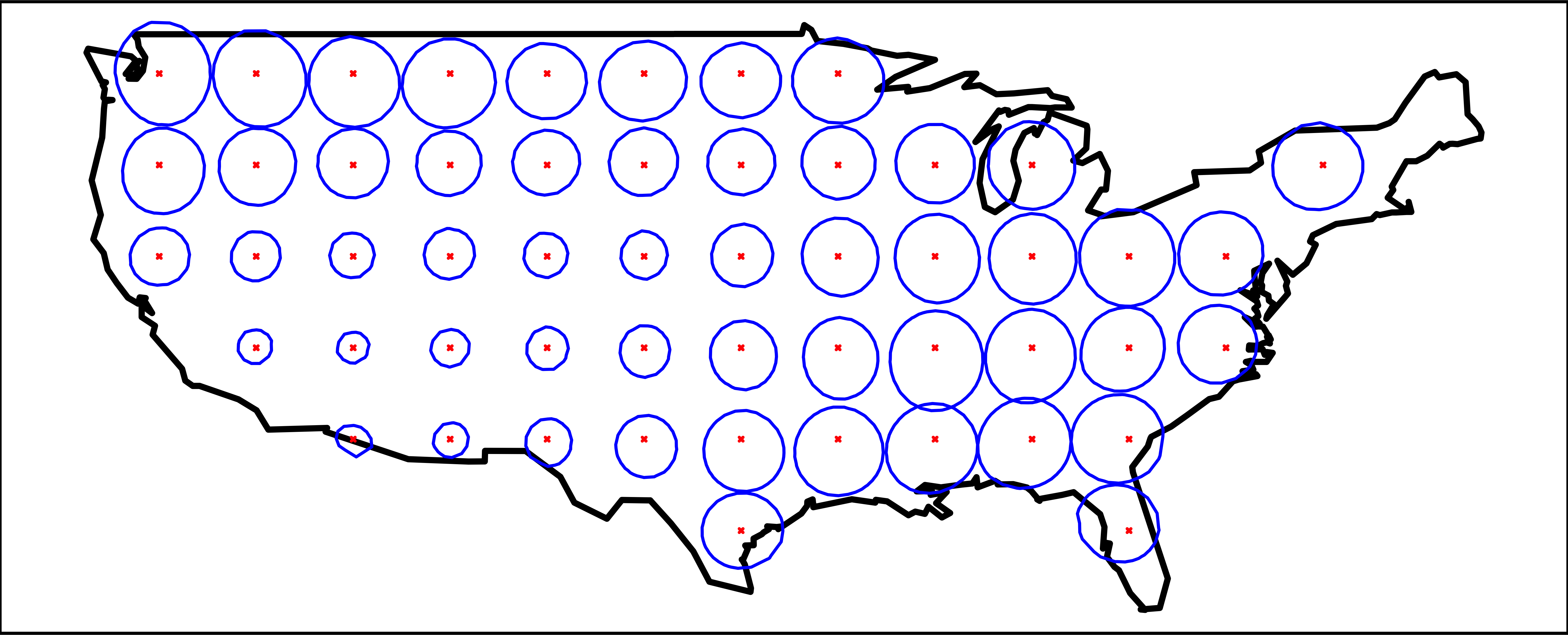
$\beta=1$ model

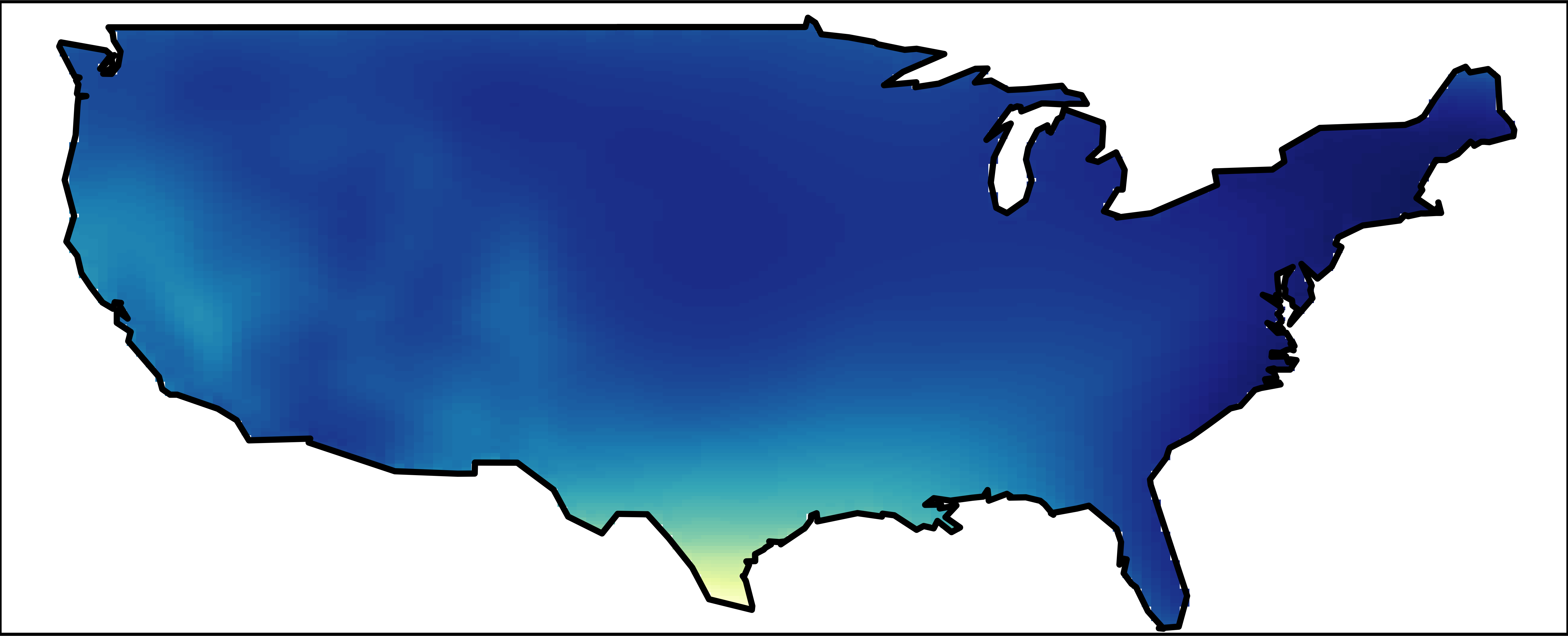
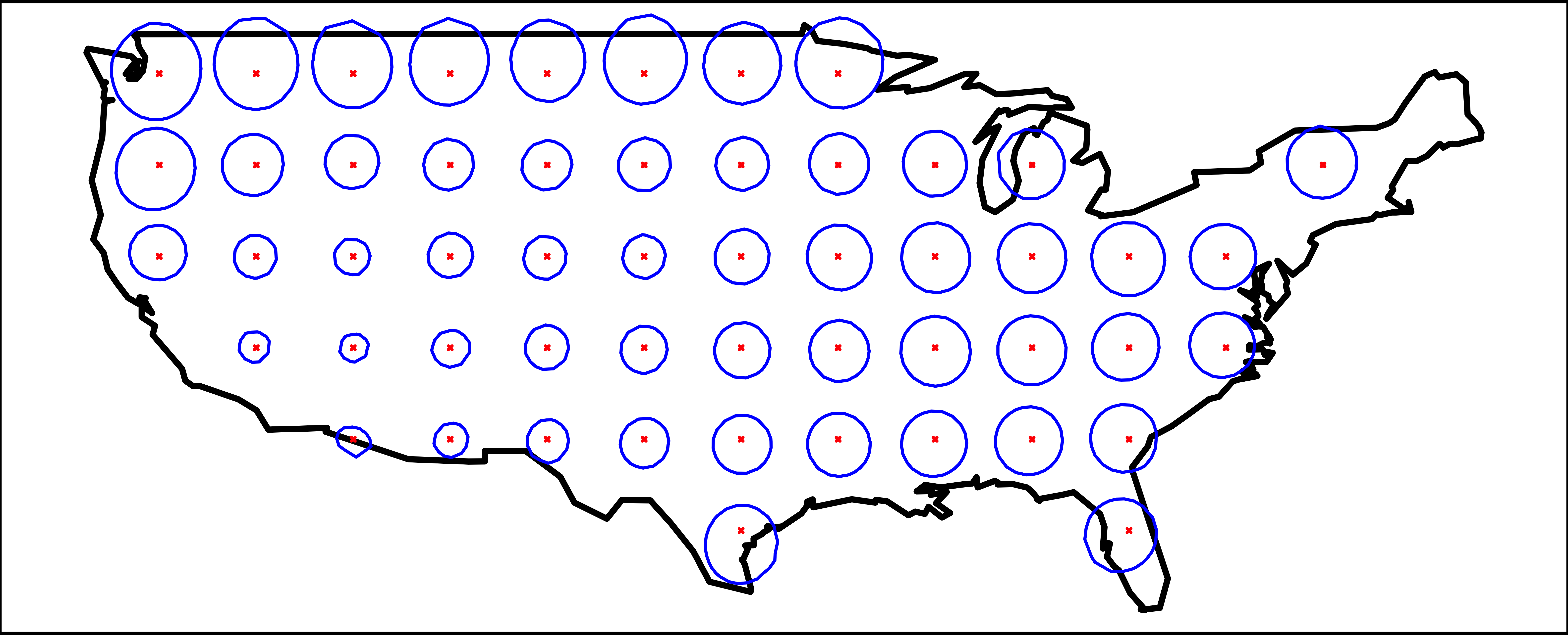
Figure 4. Estimated marginal standard deviations (top row) and contours of $0.7$ correlation of the correlation function for selected locations (bottom row), for the fractional (left column) and $\beta=1$ (right column) models.

	Log-likelihood	RMSE	CRPS	LS	Time
Stationary $\beta=1$	219773	4.206	2.295	177.2	0.125
Stationary fractional	220255	4.167	2.274	178.2	0.412
Non-stationary $\beta=1$	225969	4.194	2.266	182.1	0.121
Non-stationary fractional	226095	4.170	2.254	182.4	0.416

Table 4. Model-dependent results for (i) the log-likelihood, (ii) the pseudo cross-validation scores (RMSE, CRPS, LS, each $\times 100$) averaged over ten replicates, and (iii) the computational time for one evaluation of the likelihood averaged over $100$ computations.

To investigate the predictive accuracy of the models, a pseudo cross-validation study is performed. We choose $10\%$ of the spatial observation locations at random, and use the corresponding observations for each year to predict the values at the remaining locations. The accuracy of the four models is measured by the root mean square error (RMSE), the average continuous ranked probability score (CRPS), and the average log-score (LS). This procedure is repeated ten times, where in each iteration new locations are chosen at random to base the predictions on. The average scores for the ten iterations are shown in Table 4. Recall that low RMSE and CRPS values resp. high LS values correspond to good scores.

We observe that the predictive performance of the non-stationary non-fractional ($\beta=1$) model is similar to the stationary fractional model in terms of CRPS, and actually worse in terms of RMSE. This clearly indicates that the data should be analyzed by a fractional model. Although the non-stationary fractional model has a better performance in terms of CRPS and LS than the stationary fractional model, the difference is quite small given that the non-stationary model has $38$ parameters, compared to $4$ for the stationary model. Thus, the fractional smoothness seems to be the most important aspect for this data. The fact that the rational SPDE approach allows us to make these comparisons and to verify the smoothness parameter, for stationary and non-stationary models, is one of its most important features.

8. Discussion

We have introduced the rational SPDE approach providing a new type of computationally efficient approximations for a class of Gaussian random fields. These are based on an extension of the SPDE approach by Lindgren et al. (2011) to models with general second-order differential operators of arbitrary order $\beta>d/4$ For these approximations, explicit rates of strong convergence have been derived and we have shown how to calibrate the degree of the rational approximation with the mesh size of the FEM to achieve these rates. The results can also be combined with the results in (Bolin et al., 2018b) to obtain explicit rates of weak convergence (convergence of functionals of the random field).

Our approach can, e.g., be used to approximate stationary Matérn fields with general smoothness, and it is also directly applicable to more complicated non-stationary models, where the covariance function may be unknown. A general fractional order of the differential operator opens up for new applications of the SPDE approach, such as to Gaussian fields with exponential covariances on $\mathbb{R}^{2}$. For the Matérn model and its extensions, it furthermore facilitates likelihood-based (or Bayesian) inference of all model parameters. The specific structure of the approximation then in turn enables a combination with INLA or MCMC in situations where the Gaussian model is a part of a more complicated non-Gaussian hierarchical model.

We have illustrated the rational SPDE approach for stationary and non-stationary Matérn models. A topic for future research is to apply the approach to other random field models in statistics which are difficult to approximate by GMRFs, such as to models with long-range dependence (Lilly et al., 2017) based on the fractional Brownian motion. Another topic for future research is to modify the fractional SPDE approach by replacing the FEM basis by a multiresolution basis and to compare this approach to other multiresolution approaches such as (Katzfuss, 2017). Finally, it is also of interest to extend the method to non-Gaussian versions of the SPDE-based Matérn models (Wallin and Bolin, 2015), since the Markov approximation considered by Wallin and Bolin (2015) is only computable under the restrictive requirement $\beta\in\mathbb{N}$.

Appendix A Iterated finite element method

The rational approximation $u_{h,m}^{R}$ of the solution $u$ to (1.2) introduced in §3.3 is defined in terms of the discrete operators $P_{\ell,h}=p_{\ell}(L_{h})$ and $P_{r,h}=p_{r}(L_{h})$ via (3.5). Since the differential operator $L$ in (3.1) is of second order, their continuous counterparts $P_{\ell}=p_{\ell}(L)$ and $P_{r}=p_{r}(L)$ in (3.7) are differential operators of order $2(m+m_{\beta})$ and $2m$, respectively. Using a standard Galerkin approach for solving (3.7) would therefore require finite element basis functions $\{\varphi_{j}\}$ in the Sobolev space $H^{m+m_{\beta}}(\mathcal{D})$, which are difficult to construct in more than one space dimension. This can be avoided by using a modified version of the iterated Hilbert space approximation method by Lindgren et al. (2011), and in this section we give the details of this procedure.

Recall from §3.2 that $V_{h}\subset V$ is a finite element space with continuous piecewise linear basis functions $\{\varphi_{j}\}_{j=1}^{n_{h}}$ defined with respect to a regular triangulation $\mathcal{T}_{h}$ of the domain $\overline{\mathcal{D}}$ with mesh width $h:=\max_{T\in\mathcal{T}_{h}}\operatorname{diam}(T)$.

For computing the finite element approximation, we start by factorizing the polynomials $q_{1}$ and $q_{2}$ in the rational approximation $\hat{r}$ of $\hat{f}(x)=x^{\beta-m_{\beta}}$ in terms of their roots,

$$q_{1}(x)=\sum_{i=1}^{m}c_{i}x^{i}=c_{m}\prod_{i=1}^{m}(x-r_{1i})\quad\text{and}\quad q_{2}(x)=\sum_{j=1}^{m+1}b_{j}x^{j}=b_{m+1}\prod_{j=1}^{m+1}(x-r_{2j}).$$

We use these expressions to reformulate (3.9) as

$$x^{-\beta}=f(x^{-1})\approx\hat{r}(x^{-1})x^{-m_{\beta}}=\frac{c_{m}\prod_{i=1}^{m}(1-r_{1i}x)}{b_{m+1}x^{m_{\beta}-1}\prod_{j=1}^{m+1}(1-r_{2i}x)},$$

where, again, we have expanded the fraction with $x^{m}$. This representation shows that we can equivalently define the rational SPDE approximation $u_{h,m}^{R}$ as the solution to (3.5) with $P_{\ell,h},P_{r,h}$ redefined as $P_{\ell,h}=b_{m+1}L_{h}^{m_{\beta}-1}\prod_{j=1}^{m+1}({\color[rgb]{0,0,0}\mathrm{Id}_{h}}-r_{2j}L_{h})$ and $P_{r,h}=c_{m}\prod_{i=1}^{m}({\color[rgb]{0,0,0}\mathrm{Id}_{h}}-r_{1i}L_{h})$, where $\mathrm{Id}_{h}$ denotes the identity on $V_{h}$.

We use the formulation of (3.5) as a system outlined in (3.6): First we solve $P_{\ell,h}x_{h,m}=\mathcal{W}_{h}$ and we then compute $u_{h,m}^{R}=P_{r,h}x_{h,m}$. To this end, we define the functions $x_{k}\in L_{2}(\Omega;V_{h})$ for $k\in\{1,\ldots,m+m_{\beta}\}$ iteratively by

$$b_{m+1}({\color[rgb]{0,0,0}\mathrm{Id}_{h}}-r_{21}L_{h})x_{1} =\mathcal{W}_{h},$$

$$({\color[rgb]{0,0,0}\mathrm{Id}_{h}}-r_{2k}L_{h})x_{k} =x_{k-1},\qquad k=2,\ldots,m+1,$$

$$L_{h}x_{k} =x_{k-1},\qquad k=m+2,\ldots,m+m_{\beta},\quad\mbox{if $m_{\beta}\geq 2$,}$$

noting that $x_{m+m_{\beta}}=x_{h,m}$.

By recalling the bilinear form $a_{L}$ from (3.2) and expanding $x_{k}=\sum_{j=1}^{n_{h}}x_{kj}\varphi_{j}$ with respect to the finite element basis, we find that the stochastic weights ${\boldsymbol{\mathrm{x}}}_{k}=(x_{k1},\ldots,x_{k{n_{h}}})^{\top}$ satisfy

$$\sum_{j=1}^{n_{h}}x_{1j}\,b_{m+1}\left((\varphi_{j},\varphi_{i})_{L_{2}(\mathcal{D})}-r_{21}\,a_{L}(\varphi_{j},\varphi_{i})\right)=(\mathcal{W}_{h},\varphi_{i})_{L_{2}(\mathcal{D})},$$

$$\sum_{j=1}^{n_{h}}x_{kj}\left((\varphi_{j},\varphi_{i})_{L_{2}(\mathcal{D})}-r_{2k}\,a_{L}(\varphi_{j},\varphi_{i})\right)=\sum_{j=1}^{n_{h}}x_{k-1,j}\,(\varphi_{j},\varphi_{i})_{L_{2}(\mathcal{D})},\,\,2\leq k\leq m+1,$$

$$\sum_{j=1}^{n_{h}}x_{kj}\,a_{L}(\varphi_{j},\varphi_{i})=\sum_{j=1}^{n_{h}}x_{k-1,j}\,(\varphi_{j},\varphi_{i})_{L_{2}(\mathcal{D})},\quad k=m+2,\ldots,m+m_{\beta},$$

where each of these equations hold for $i=1,\ldots,n_{h}$. Recall from §3.2 that $\mathcal{W}_{h}$ is white noise in $V_{h}$. This entails the distribution $\bigl{(}(\mathcal{W}_{h},\varphi_{i})_{L_{2}(\mathcal{D})}\bigr{)}_{i=1}^{n_{h}}\sim\mathsf{N}({\boldsymbol{\mathrm{0}}},{\boldsymbol{\mathrm{C}}})$, where ${\boldsymbol{\mathrm{C}}}$ is the mass matrix with elements $C_{ij}=(\varphi_{j},\varphi_{i})_{L_{2}(\mathcal{D})}$ and, therefore, ${\boldsymbol{\mathrm{x}}}_{k}\sim\mathsf{N}\bigl{(}{\boldsymbol{\mathrm{0}}},{\boldsymbol{\mathrm{P}}}_{\ell,k}^{-1}{\boldsymbol{\mathrm{C}}}{\boldsymbol{\mathrm{P}}}_{\ell,k}^{-\top}\bigr{)}$ for every $k\in\{1,...,m+m_{\beta}\}$. Here, the matrix ${\boldsymbol{\mathrm{P}}}_{\ell,k}$ is defined by

$${\boldsymbol{\mathrm{P}}}_{\ell,k}=\begin{cases}b_{m+1}{\boldsymbol{\mathrm{C}}}\,{\boldsymbol{\mathrm{L}}}_{k},&k=1,\ldots,m+1,\\ b_{m+1}{\boldsymbol{\mathrm{C}}}\left({\boldsymbol{\mathrm{C}}}^{-1}{\boldsymbol{\mathrm{L}}}\right)^{k-m-1}{\boldsymbol{\mathrm{L}}}_{m+1},&k=m+2,\ldots,m+m_{\beta},\end{cases}$$

where ${\boldsymbol{\mathrm{L}}}_{k}:=\prod_{j=1}^{k}\left({\boldsymbol{\mathrm{I}}}-r_{2j}{\boldsymbol{\mathrm{C}}}^{-1}{\boldsymbol{\mathrm{L}}}\right)$, with identity matrix ${\boldsymbol{\mathrm{I}}}\in\mathbb{R}^{n_{h}\times n_{h}}$, and the entries of ${\boldsymbol{\mathrm{L}}}$ are given by

$$L_{ij}:=a_{L}(\varphi_{j},\varphi_{i})=({\boldsymbol{\mathrm{H}}}\nabla\varphi_{j},\nabla\varphi_{i})_{L_{2}(\mathcal{D})}+\left(\kappa^{2}\varphi_{j},\varphi_{i}\right)_{L_{2}(\mathcal{D})},\qquad i,j=1,\ldots,n_{h},$$

cf. (3.1)–(3.2). In particular, the weights ${\boldsymbol{\mathrm{x}}}$ of $x_{h,m}$ have distribution

$${\boldsymbol{\mathrm{x}}}\sim\mathsf{N}\left({\boldsymbol{\mathrm{0}}},{\boldsymbol{\mathrm{P}}}_{\ell}^{-1}{\boldsymbol{\mathrm{C}}}{\boldsymbol{\mathrm{P}}}_{\ell}^{-\top}\right),\qquad\text{where}\qquad{\boldsymbol{\mathrm{P}}}_{\ell}:={\boldsymbol{\mathrm{P}}}_{\ell,m+m_{\beta}}.$$ (A.1)

Note also that for the Matérn case, i.e., $L=\kappa^{2}-\Delta$, we have ${\boldsymbol{\mathrm{L}}}=\kappa^{2}{\boldsymbol{\mathrm{C}}}+{\boldsymbol{\mathrm{G}}}$, where ${\boldsymbol{\mathrm{G}}}$ is the stiffness matrix with elements $G_{ij}=(\nabla\varphi_{j},\nabla\varphi_{i})_{L_{2}(\mathcal{D})}$.

To calculate the final approximation $u_{h,m}^{R}=P_{r,h}x_{h,m}$, we apply a similar iterative procedure. Let $u_{1},\ldots,u_{m}$ be defined by

$$u_{1} =c_{m}({\color[rgb]{0,0,0}\mathrm{Id}_{h}}-r_{11}L_{h})x_{h,m},$$

$$u_{k} =({\color[rgb]{0,0,0}\mathrm{Id}_{h}}-r_{1k}L_{h})u_{k-1},\qquad\quad k=2,\ldots,m.$$

Then $u_{h,m}^{R}=c_{m}\bigl{(}\prod_{i=1}^{m}(\mathrm{Id}-r_{1i}L_{h})\bigr{)}x_{h,m}=u_{m}$ and the weights ${\boldsymbol{\mathrm{u}}}_{k}$ of $u_{k}$ can be obtained from the weights of $x_{h,m}$ via ${\boldsymbol{\mathrm{u}}}_{k}={\boldsymbol{\mathrm{P}}}_{r,k}\,{\boldsymbol{\mathrm{x}}}$, where

$${\boldsymbol{\mathrm{P}}}_{r,k}:=c_{m}\prod_{i=1}^{k}\left({\boldsymbol{\mathrm{I}}}-r_{1i}{\boldsymbol{\mathrm{C}}}^{-1}{\boldsymbol{\mathrm{L}}}\right).$$

By (A.1), the distribution of the weights ${\boldsymbol{\mathrm{u}}}$ of the final rational approximation $u_{h,m}^{R}$ is thus given by

$${\boldsymbol{\mathrm{u}}}\sim\mathsf{N}\left({\boldsymbol{\mathrm{0}}},{\boldsymbol{\mathrm{P}}}_{r}{\boldsymbol{\mathrm{P}}}_{\ell}^{-1}{\boldsymbol{\mathrm{C}}}{\boldsymbol{\mathrm{P}}}_{\ell}^{-\top}{\boldsymbol{\mathrm{P}}}_{r}^{\top}\right),\qquad\text{where}\qquad{\boldsymbol{\mathrm{P}}}_{r}:={\boldsymbol{\mathrm{P}}}_{r,m}.$$

To obtain sparse matrices ${\boldsymbol{\mathrm{P}}}_{\ell}$ and ${\boldsymbol{\mathrm{P}}}_{r}$, we approximate the mass matrix ${\boldsymbol{\mathrm{C}}}$ by a diagonal matrix $\widetilde{{\boldsymbol{\mathrm{C}}}}$ with diagonal elements $\widetilde{C}_{ii}=\sum_{j=1}^{n_{h}}C_{ij}$. The effect of this “mass lumping” was motivated theoretically by Lindgren et al. (2011), and was empirically shown to be small by Bolin and Lindgren (2013).

Appendix B Convergence analysis

In this section we give the details of the convergence result stated in Theorem 3.3. As mentioned in §3.4, we choose $\hat{r}=\hat{r}_{h}$ as the $L_{\infty}$-best rational approximation of $\hat{f}(x)=x^{\beta-m_{\beta}}$ on the interval $J_{h}$ for each $h$. We furthermore assume that the operator $L$ in (3.1) is normalized such that $\lambda_{1}\geq 1$ and, thus, $J_{h}\subset J\subset[0,1]$.

Recall that Proposition 3.2 provides a bound for $\|u-u_{h}\|_{L_{2}(\Omega;L_{2}(\mathcal{D}))}$. Therefore, it remains is to estimate the strong error between $u_{h,m}^{R}$ and $u_{h}$ induced by the rational approximation of $f(x)=x^{\beta}$. To this end, recall the construction of the rational approximation $u_{h,m}^{R}$ from §3.3: We first decomposed $f$ as $f(x)=\hat{f}(x)x^{m_{\beta}}$, where $\hat{f}(x)=x^{\beta-m_{\beta}}$, and then used a rational approximation $\hat{r}=\frac{q_{1}}{q_{2}}$ of $\hat{f}$ on the interval $J_{h}=\bigl{[}\lambda_{n_{h},h}^{-1},\lambda_{1,h}^{-1}\bigr{]}$ with $q_{1}\in\mathcal{P}^{m}(J_{h})$ and $q_{2}\in\mathcal{P}^{m+1}(J_{h})$ to define the approximation $r(x):=\hat{r}(x)x^{m_{\beta}}$ of $f$. Here, $\mathcal{P}^{m}(J_{h})$ denotes the set of polynomials $q\colon J_{h}\to\mathbb{R}$ of degree $\deg(q)=m$. In the following, we assume that $\hat{r}=\hat{r}_{h}$ is the best rational approximation of $\hat{f}$ of this form, i.e.,

$$\|\hat{f}-\hat{r}_{h}\|_{C(J_{h})}=\inf\left\{\|\hat{f}-\hat{\rho}\|_{C(J_{h})}:\hat{\rho}=\tfrac{q_{1}}{q_{2}},\ q_{1}\in\mathcal{P}^{m}(J_{h}),\ q_{2}\in\mathcal{P}^{m+1}(J_{h})\right\},$$

where $\|g\|_{C(J)}:=\sup_{x\in J}|g(x)|$.

For the analysis, we treat the two cases $\beta\in(0,1)$ and $\beta\geq 1$ separately. If $\beta\geq 1$, then $\hat{\beta}:=\beta-m_{\beta}\in[0,1)$. Thus, if $\hat{r}_{*}$ denotes the best rational approximation of $\hat{f}$ on the interval $[0,1]$, we find (Stahl, 2003, Theorem 1)

$$\|\hat{f}-\hat{r}_{h}\|_{C(J_{h})}\leq\sup_{x\in[0,1]}|\hat{f}(x)-\hat{r}_{*}(x)|\leq\hat{C}e^{-2\pi\sqrt{\hat{\beta}m}},$$

where the constant $\hat{C}>0$ is continuous in $\hat{\beta}$ and independent of $h$ and the degree $m$. Since $x^{m_{\beta}}\leq 1$ for all $x\in J_{h}$, we obtain for $r_{h}(x):=\hat{r}_{h}(x)x^{m_{\beta}}$ the same bound,

$$\|f-r_{h}\|_{C(J_{h})}\leq\sup_{x\in J_{h}}|\hat{f}(x)-\hat{r}_{h}(x)|\leq\hat{C}e^{-2\pi\sqrt{\hat{\beta}m}}.$$ (B.1)

If $\beta\in(0,1)$, then $\hat{\beta}\in(-1,0)$ and we let $\widetilde{r}$ be the best approximation of $\widetilde{f}(x):=x^{|\hat{\beta}|}$ on $[0,1]$. A rational approximation of $\widetilde{f}$ on the different interval $\widetilde{J}_{h}:=[\lambda_{1,h},\lambda_{n_{h},h}]$ is then given by $\widetilde{R}_{h}(\widetilde{x}):=\lambda_{n_{h},h}^{|\hat{\beta}|}\widetilde{r}(\lambda_{n_{h},h}^{-1}\widetilde{x})$ with error

$$\sup_{\widetilde{x}\in\widetilde{J}_{h}}|\widetilde{f}(\widetilde{x})-\widetilde{R}_{h}(\widetilde{x})|\leq\lambda_{n_{h},h}^{|\hat{\beta}|}\sup_{x\in[0,1]}|\widetilde{f}(x)-\widetilde{r}(x)|\leq\widetilde{C}\lambda_{n_{h},h}^{|\hat{\beta}|}e^{-2\pi\sqrt{|\hat{\beta}|m}},$$

where the constant $\widetilde{C}>0$ depends only on $|\hat{\beta}|$. On $J_{h}=\bigl{[}\lambda_{n_{h},h}^{-1},\lambda_{1,h}^{-1}\bigr{]}$ the function $\widetilde{R}_{h}(x^{-1})$ is an approximation of $\hat{f}(x)=x^{\hat{\beta}}=\widetilde{f}(x^{-1})$ and

$$\|\hat{f}-\hat{r}_{h}\|_{C(J_{h})}\leq\sup_{x\in J_{h}}|\hat{f}(x)-\widetilde{R}_{h}(x^{-1})|\leq\sup_{\widetilde{x}\in\widetilde{J}_{h}}|\widetilde{f}(\widetilde{x})-\widetilde{R}_{h}(\widetilde{x})|\leq\widetilde{C}\lambda_{n_{h},h}^{|\hat{\beta}|}e^{-2\pi\sqrt{|\hat{\beta}|m}}.$$

Finally, we use again the estimate $x^{m_{\beta}}\leq 1$ on $J_{h}$ to derive

$$\|f-r_{h}\|_{C(J_{h})}\leq\|\hat{f}-\hat{r}_{h}\|_{C(J_{h})}\leq\widetilde{C}\lambda_{n_{h},h}^{|\hat{\beta}|}e^{-2\pi\sqrt{|\hat{\beta}|m}}.$$ (B.2)

Proposition 3.2 and the estimates (B.1)–(B.2) yield Theorem 3.3, which is proven below.

Proof of Theorem 3.3.

By Proposition 3.2, it suffices to bound $\mathbb{E}\|u_{h}-u_{h,m}^{R}\|_{L_{2}(\mathcal{D})}^{2}$. To this end, let $\mathcal{W}_{h}=\sum_{j=1}^{n_{h}}\xi_{j}e_{j,h}$ be a Karhunen–Loève expansion of $\mathcal{W}_{h}$, where $\{e_{j,h}\}_{j=1}^{n_{h}}$ are $L_{2}(\mathcal{D})$-orthonormal eigenvectors of $L_{h}$ corresponding to the eigenvalues $\{\lambda_{j,h}\}_{j=1}^{n_{h}}$ and $\xi_{j}\sim\mathsf{N}(0,1)$ i.i.d..

By construction and owing to boundedness and invertibility of $L_{h}$, we have for $u_{h,m}^{R}$ in (3.5) that $u_{h,m}^{R}=P_{\ell,h}^{-1}P_{r,h}\mathcal{W}_{h}=r_{h}(L_{h}^{-1})\mathcal{W}_{h}$ and we estimate

$$\mathbb{E}\|u_{h}-u_{h,m}^{R}\|_{L_{2}(\mathcal{D})}^{2} =\mathbb{E}\sum_{j=1}^{n_{h}}\xi_{j}^{2}\left(\lambda_{j,h}^{-\beta}-r_{h}(\lambda_{j,h}^{-1})\right)^{2}\leq n_{h}\max_{1\leq j\leq n_{h}}\bigl{|}\lambda_{j,h}^{-\beta}-r_{h}(\lambda_{j,h}^{-1})\bigr{|}^{2}.$$

By (B.1) and (B.2), we can bound the last term by

$$\max_{1\leq j\leq n_{h}}\bigl{|}\lambda_{j,h}^{-\beta}-r_{h}(\lambda_{j,h}^{-1})\bigr{|}^{2} \leq\left(\sup_{x\in J_{h}}|f(x)-r_{h}(x)|\right)^{2}\lesssim\lambda_{n_{h},h}^{2\max\{(1-\beta),0\}}e^{-4\pi\sqrt{|\beta-m_{\beta}|m}}.$$

By (Strang and Fix, 2008, Theorem 6.1) we have $\lambda_{n_{h},h}\lesssim\lambda_{n_{h}}\lesssim n_{h}^{2/d}$, for sufficiently small $h\in(0,1)$, where the last bound follows from the Weyl asymptotic (3.3). Finally, $n_{h}\lesssim h^{-d}$ by quasi-uniformity of the triangulation $\mathcal{T}_{h}$. Thus, we conclude

$$\mathbb{E}\|u_{h}-u_{h,m}^{R}\|_{L_{2}(\mathcal{D})}^{2} \lesssim h^{-4\max\{(1-\beta),\,0\}-d}e^{-4\pi\sqrt{|\beta-m_{\beta}|m}},$$

which combined with Proposition 3.2 proves Theorem 3.3. ∎

Appendix C A comparison to the quadrature approach

Bolin et al. (2018a) proposed another method which can be applied to simulate the solution $u$ to (1.2) numerically. The approach therein is to express the discretized equation (3.4) as $L_{h}^{\tilde{\beta}}L_{h}^{\lfloor\beta\rfloor}u_{h}=\mathcal{W}_{h}$, where $\tilde{\beta}=\beta-\lfloor\beta\rfloor\in[0,1)$. Since $L_{h}^{\lfloor\beta\rfloor}u_{h}=f$ can be solved by using non-fractional methods, the focus was on the fractional case $\beta\in(0,1)$ when constructing the approximative solution. From the Dunford–Taylor calculus (Yosida, 1995, §IX.11) one has in this case the following representation of the discrete inverse,

$$L_{h}^{-\beta} =\frac{\sin(\pi\beta)}{\pi}\int_{0}^{\infty}\lambda^{-\beta}\left(\lambda\,{\color[rgb]{0,0,0}\mathrm{Id}_{h}}+L_{h}\right)^{-1}\,\mathrm{d}\lambda.$$

Bonito and Pasciak (2015) introduced a quadrature approximation $Q_{h,k}^{\beta}$ of this integral after a change of variables $\lambda=e^{-2y}$ and based on an equidistant grid for $y$ with step size $k>0$, i.e.,

$$Q_{h,k}^{\beta}:=\frac{2k\sin(\pi\beta)}{\pi}\sum_{j=-K^{-}}^{K^{+}}e^{2\beta y_{j}}\left({\color[rgb]{0,0,0}\mathrm{Id}_{h}}+e^{2y_{j}}L_{h}\right)^{-1},\quad\text{where}\quad y_{j}:=jk.$$

Exponential convergence of order $\mathcal{O}\bigl{(}e^{-\pi^{2}/(2k)}\bigr{)}$ of the operator $Q_{h,k}^{\beta}$ to the discrete fractional inverse $L_{h}^{-\beta}$ was proven for $K^{-}:=\left\lceil\frac{\pi^{2}}{4\beta k^{2}}\right\rceil$ and $K^{+}:=\left\lceil\frac{\pi^{2}}{4(1-\beta)k^{2}}\right\rceil$.

By calibrating the number of quadrature nodes with the number of basis functions in the FEM, an explicit rate of convergence for the strong error of the approximation $u_{h,k}^{Q}=Q_{h,k}^{\beta}\mathcal{W}_{h}$ was derived (Bolin et al., 2018a, Theorem 2.10). Motivated by the asymptotic convergence of the method, it was suggested to choose $k\leq-\tfrac{\pi^{2}}{4\beta\ln(h)}$ in order to balance the errors induced by the quadrature and by a FEM of mesh size $h$ (Bolin et al., 2018a, Table 1). This corresponds to a total number of $K=K^{-}+K^{+}+1>\tfrac{4\beta\ln(h)^{2}}{\pi^{2}(1-\beta)}$ quadrature nodes. The analogous result for the degree $m$ of the approximation $u_{h,m}^{R}$ is given in Remark 3.4, suggesting the lower bound $m\geq\tfrac{\ln(h)^{2}}{\pi^{2}(1-\beta)}$, i.e., $K=4\beta m$ asymptotically.

Furthermore, if we let $c_{j}:=e^{2y_{j}}$ and

$$P_{\ell,h}^{Q}:=\prod_{j=-K^{-}}^{K^{+}}c_{j}^{-\beta}\left(\mathrm{Id}_{h}+c_{j}L_{h}\right),\quad P_{r,h}^{Q}:=\frac{2k\sin(\pi\beta)}{\pi}\sum_{i=-K^{-}}^{K^{+}}\prod_{j\neq i}c_{j}^{-\beta}\left(\mathrm{Id}_{h}+c_{j}L_{h}\right),$$

we find that the quadrature-based approximation $u_{h,k}^{Q}$ can equivalently be defined as the solution to the non-fractional SPDE

$$P_{\ell,h}^{Q}u_{h,k}^{Q}=P_{r,h}^{Q}\mathcal{W}_{h}\quad\text{in }\mathcal{D}.$$ (C.1)

Remark C.1.

A comparison of (C.1) with (3.5) illustrates that $u_{h,k}^{Q}$ can be seen as a rational approximation of degree $K^{-}+K^{+}$, where the specific choice of the coefficients is implied by the quadrature. In combination with the remark above that $K=4\beta m$ quadrature nodes are needed to balance the errors, this shows that the computational cost for achieving a given accuracy with the rational approximation from §3.3 is lower than with the quadrature method, since $\beta>d/4$.

Appendix D Parameter identifiability

This section contains the proof of Theorem 6.1. For the proof, we will use the Feldman–Hájek theorem which we restate here from (Da Prato and Zabczyk, 2014, Theorem 2.25) for convenience.

Theorem D.1 (Felman–Hájek).

Two Gaussian measures $\mu_{1}=\mathsf{N}(m_{1},\mathcal{C}_{1})$ and $\mu_{2}=\mathsf{N}(m_{2},\mathcal{C}_{2})$ on a Hilbert space $\mathcal{H}$ are either singular or equivalent. They are equivalent if and only if the following three conditions are satisfied:

1. $\operatorname{Im}\bigl{(}\mathcal{C}_{1}^{1/2}\bigr{)}=\operatorname{Im}\bigl{(}\mathcal{C}_{2}^{1/2}\bigr{)}:=E$,

2. $m_{1}-m_{2}\in E$,

3. the operator $T:=\bigl{(}\mathcal{C}_{1}^{-1/2}\mathcal{C}_{2}^{1/2}\bigr{)}\bigl{(}\mathcal{C}_{1}^{-1/2}\mathcal{C}_{2}^{1/2}\bigr{)}^{*}-I$ is Hilbert-Schmidt in $\bar{E}$, where $*$ denotes the $\mathcal{H}$-adjoint operator, and $I$ the identity on $\mathcal{H}$.

Proof of Theorem 6.1.

Since the two Gaussian measures have the same mean, we only have to verify conditions I. and III. of Theorem D.1.

We first prove that condition I. can hold only if $\beta_{1}=\beta_{2}$. To this end, we use the equivalence of condition I. with the existence of two constants $c^{\prime},c^{\prime\prime}>0$ such that

$$(v,\mathcal{C}_{1}v)_{L_{2}(\mathcal{D})}\leq c^{\prime}(v,\mathcal{C}_{2}v)_{L_{2}(\mathcal{D})}\quad\text{and}\quad(v,\mathcal{C}_{2}v)_{L_{2}(\mathcal{D})}\leq c^{\prime\prime}(v,\mathcal{C}_{1}v)_{L_{2}(\mathcal{D})},$$ (D.1)

see, e.g., (Stuart, 2010, Lemma 6.15), where in our case

$$\mathcal{C}_{i}:=\mathcal{Q}_{i}^{-1}=\tau_{i}^{-2}(\kappa_{i}^{2}-\Delta)^{-2\beta_{i}},\qquad i\in\{1,2\}.$$

Let $\lambda_{j}^{\Delta}$, $j\in\mathbb{N}$, denote the positive eigenvalues (in nondecreasing order, counting multiplicity) of the Dirichlet or Neumann Laplacian $-\Delta\colon\mathscr{D}(\Delta)\to L_{2}(\mathcal{D})$, where the type of homogeneous boundary conditions is the same as for $L_{1}$ and $L_{2}$. By Weyl’s law (3.3), there exist constants $\underline{c},\bar{C}>0$ such that

$$\underline{c}\,j^{2/d}\leq\lambda_{j}^{\Delta}\leq\bar{C}j^{2/d}\qquad\forall j\in\mathbb{N}.$$

Furthermore, we let $\{e_{j}\}_{j\in\mathbb{N}}$ denote a system of eigenfunctions corresponding to $\bigl{\{}\lambda_{j}^{\Delta}\bigr{\}}_{j\in\mathbb{N}}$ which is orthonormal in $L_{2}(\mathcal{D})$.

Now assume that $\beta_{2}>\beta_{1}$ and let $j_{0}\in\mathbb{N}$ be sufficiently large such that $\kappa_{1}^{2}<\bar{C}j_{0}^{2/d}$. Then, we have

$$\frac{(\kappa_{2}^{2}+\lambda_{j}^{\Delta})^{2\beta_{2}}}{(\kappa_{1}^{2}+\lambda_{j}^{\Delta})^{2\beta_{1}}}>\frac{\underline{c}^{2\beta_{2}}}{(2\bar{C})^{2\beta_{1}}}\,j^{4(\beta_{2}-\beta_{1})/d}\qquad\forall j\in\mathbb{N},\ j\geq j_{0}.$$

For any $N\in\mathbb{N}$, we can thus choose $j_{*}=j_{*}(N)\in\mathbb{N}$ sufficiently large such that

$$(e_{j_{*}},\mathcal{C}_{1}e_{j_{*}})_{L_{2}(\mathcal{D})}=\tau_{1}^{-2}(\kappa_{1}^{2}+\lambda_{j_{*}}^{\Delta})^{-2\beta_{1}}>N\tau_{2}^{-2}(\kappa_{2}^{2}+\lambda_{j_{*}}^{\Delta})^{-2\beta_{2}}=N(e_{j_{*}},\mathcal{C}_{2}e_{j_{*}})_{L_{2}(\mathcal{D})},$$

in contradiction with the first relation in (D.1), and $\mu_{1},\mu_{2}$ are not equivalent if $\beta_{1}\neq\beta_{2}$. Furthermore, condition I. is satisfied if $\beta_{1}=\beta_{2}=\beta>d/4$, since then, for all $v\in L_{2}(\mathcal{D})$,

$$(v,\mathcal{C}_{1}v)_{L_{2}(\mathcal{D})} =\sum_{j\in\mathbb{N}}\tau_{1}^{-2}(\kappa_{1}^{2}+\lambda_{j}^{\Delta})^{-2\beta}(v,e_{j})_{L_{2}(\mathcal{D})}^{2}$$

$$\leq\tau_{1}^{-2}\tau_{2}^{2}\left(\min\left\{1,\kappa_{1}^{2}\kappa_{2}^{-2}\right\}\right)^{-2\beta}\sum_{j\in\mathbb{N}}\tau_{2}^{-2}(\kappa_{2}^{2}+\lambda_{j}^{\Delta})^{-2\beta}(v,e_{j})_{L_{2}(\mathcal{D})}^{2}$$

$$=\tau_{1}^{-2}\tau_{2}^{2}\max\left\{1,\kappa_{1}^{-4\beta}\kappa_{2}^{4\beta}\right\}(v,\mathcal{C}_{2}v)_{L_{2}(\mathcal{D})},$$

and, similarly, $(v,\mathcal{C}_{2}v)_{L_{2}(\mathcal{D})}\leq\tau_{2}^{-2}\tau_{1}^{2}\max\bigl{\{}1,\kappa_{2}^{-4\beta}\kappa_{1}^{4\beta}\bigr{\}}(v,\mathcal{C}_{1}v)_{L_{2}(\mathcal{D})}$. Thus, (D.1) and condition I. of Theorem D.1 hold.

Assuming that $\beta_{1}=\beta_{2}=\beta>d/4$, it remains now to show that condition III. of Theorem D.1 is satisfied if and only if $\tau_{1}=\tau_{2}$. To this end, we first note that the operator $T:=\mathcal{C}_{1}^{-1/2}\mathcal{C}_{2}\mathcal{C}_{1}^{-1/2}-I$ has eigenfunctions $\{e_{j}\}_{j\in\mathbb{N}}$ and eigenvalues

$$\tau_{1}^{2}\tau_{2}^{-2}(\kappa_{1}^{2}+\lambda_{j}^{\Delta})^{2\beta}(\kappa_{2}^{2}+\lambda_{j}^{\Delta})^{-2\beta}-1,\qquad j\in\mathbb{N}.$$

Therefore, $T$ is Hilbert–Schmidt in $\bar{E}$ if and only if

$$\sum_{j\in\mathbb{N}}\left(\tau_{1}^{2}\tau_{2}^{-2}(\kappa_{1}^{2}+\lambda_{j}^{\Delta})^{2\beta}(\kappa_{2}^{2}+\lambda_{j}^{\Delta})^{-2\beta}-1\right)^{2}<\infty.$$ (D.2)

Since $x\mapsto(1+x)^{1/(2\beta)}$ is monotonically increasing in $x>0$, again by the Weyl asymptotic, for any $\varepsilon_{0}>0$, we can find an index $j_{0}\in\mathbb{N}$ such that

$$\frac{\kappa_{2}^{2}}{\lambda_{j}^{\Delta}}+1\leq(1+\varepsilon_{0})^{1/(2\beta)}\qquad\forall j\in\mathbb{N},\ j\geq j_{0}.$$ (D.3)

Assume that $\tau_{1}\neq\tau_{2}$ and without loss of generality let $\tau_{1}>\tau_{2}$. Then pick $\varepsilon_{0}>0$ such that $\tau_{1}^{2}\tau_{2}^{-2}\geq 1+2\varepsilon_{0}$, and $j_{0}\in\mathbb{N}$ such that (D.3) holds. These choices give

$$\tau_{1}^{2}\tau_{2}^{-2}\left(\frac{\kappa_{1}^{2}+\lambda_{j}^{\Delta}}{\kappa_{2}^{2}+\lambda_{j}^{\Delta}}\right)^{2\beta}\geq\tau_{1}^{2}\tau_{2}^{-2}(\kappa_{2}^{2}/\lambda_{j}^{\Delta}+1)^{-2\beta}\geq(1+2\varepsilon_{0})(1+\varepsilon_{0})^{-1}>1,$$

for all $j\in\mathbb{N}$ with $j\geq j_{0}$. Thus, the series in (D.2) is unbounded,

$$\sum_{j\in\mathbb{N}}\left(\tau_{1}^{2}\tau_{2}^{-2}(\kappa_{1}^{2}+\lambda_{j}^{\Delta})^{2\beta}(\kappa_{2}^{2}+\lambda_{j}^{\Delta})^{-2\beta}-1\right)^{2} \geq\sum_{j\geq j_{0}}\left((1+2\varepsilon_{0})(1+\varepsilon_{0})^{-1}-1\right)^{2}$$

$$=\sum_{j\geq j_{0}}\varepsilon_{0}^{2}\left(1+\varepsilon_{0}\right)^{-2}=\infty.$$

We conclude that condition III. of Theorem D.1 is not satisfied if $\tau_{1}\neq\tau_{2}$.

Finally, let $\beta_{1}=\beta_{2}=\beta$, $\tau_{1}=\tau_{2}$ and assume without loss of generality that $\kappa_{2}>\kappa_{1}$ (if $\kappa_{1}=\kappa_{2}$, (D.2) is evident). By the mean value theorem, applied for the function $x\mapsto x^{2\beta}$, for every $j\in\mathbb{N}$, there exists $\widetilde{\kappa}_{j}\in(\kappa_{1},\kappa_{2})$ such that

$$(\kappa_{2}^{2}+\lambda_{j}^{\Delta})^{2\beta}-(\kappa_{1}^{2}+\lambda_{j}^{\Delta})^{2\beta}=2\beta(\widetilde{\kappa}_{j}^{2}+\lambda_{j}^{\Delta})^{2\beta-1}(\kappa_{2}^{2}-\kappa_{1}^{2}).$$

Hence, we can bound the series in (D.2) as follows,

$$\sum_{j\in\mathbb{N}} \left(\frac{(\kappa_{1}^{2}+\lambda_{j}^{\Delta})^{2\beta}-(\kappa_{2}^{2}+\lambda_{j}^{\Delta})^{2\beta}}{(\kappa_{2}^{2}+\lambda_{j}^{\Delta})^{2\beta}}\right)^{2}=4\beta^{2}(\kappa_{2}^{2}-\kappa_{1}^{2})^{2}\sum_{j\in\mathbb{N}}\left(\frac{(\widetilde{\kappa}_{j}^{2}+\lambda_{j}^{\Delta})^{2\beta-1}}{(\kappa_{2}^{2}+\lambda_{j}^{\Delta})^{2\beta}}\right)^{2}$$

$$\leq 4\beta^{2}(\kappa_{2}^{2}-\kappa_{1}^{2})^{2}\sum_{j\in\mathbb{N}}(\widetilde{\kappa}_{j}^{2}+\lambda_{j}^{\Delta})^{-2}\leq 4\beta^{2}(\kappa_{2}^{2}-\kappa_{1}^{2})^{2}\underline{c}^{-2}\sum_{j\in\mathbb{N}}j^{-4/d}<\infty.$$

Here, $\sum_{j\in\mathbb{N}}j^{-4/d}$ converges, since $4/d>1$ for $d\in\{1,2,3\}$. This proves equivalence of the Gaussian measures if $\beta_{1}=\beta_{2}$ and $\tau_{1}=\tau_{2}$. ∎

References

- Baker and Graves-Morris (1996) Baker, Jr., G. A. and Graves-Morris, P. (1996). Padé approximants, volume 59 of Encyclopedia of Mathematics and its Applications. Cambridge University Press, second edition.
- Bakka et al. (2018) Bakka, H., Rue, H., Fuglstad, G.-A., Riebler, A., Bolin, D., Illian, J., Krainski, E., Simpson, D., and Lindgren, F. (2018). Spatial modelling with R-INLA: A review. WIREs Comput. Stat., 10(6):e1443.
- Bakka et al. (2019) Bakka, H., Vanhatalo, J., Illian, J. B., Simpson, D., and Rue, H. (2019). Non-stationary Gaussian models with physical barriers. Spat. Stat., 29:268–288.
- Bolin (2019) Bolin, D. (2019). rSPDE: Rational approximations of fractional SPDEs. R package version 0.4.6, https://CRAN.R-project.org/package=rSPDE.
- Bolin et al. (2018a) Bolin, D., Kirchner, K., and Kovács, M. (2018a). Numerical solution of fractional elliptic stochastic PDEs with spatial white noise. IMA J. Numer. Anal., n/a:n/a–n/a. Electronic.
- Bolin et al. (2018b) Bolin, D., Kirchner, K., and Kovács, M. (2018b). Weak convergence of galerkin approximations for fractional elliptic stochastic pdes with spatial white noise. BIT Numer. Math., 58(4):881–906.
- Bolin and Lindgren (2013) Bolin, D. and Lindgren, F. (2013). A comparison between Markov approximations and other methods for large spatial data sets. Comput. Statist. Data Anal., 61:7–21.