Neural Natural Language Inference Models Enhanced with
External Knowledge

Abstract

Modeling natural language inference is a very challenging task. With the availability of large annotated data, it has recently become feasible to train complex models such as neural-network-based inference models, which have shown to achieve the state-of-the-art performance. Although there exist relatively large annotated data, can machines learn all knowledge needed to perform natural language inference (NLI) from these data? If not, how can neural-network-based NLI models benefit from external knowledge and how to build NLI models to leverage it? In this paper, we enrich the state-of-the-art neural natural language inference models with external knowledge. We demonstrate that the proposed models improve neural NLI models to achieve the state-of-the-art performance on the SNLI and MultiNLI datasets.

1 Introduction

Reasoning and inference are central to both human and artificial intelligence. Natural language inference (NLI), also known as recognizing textual entailment (RTE), is an important NLP problem concerned with determining inferential relationship (e.g., entailment, contradiction, or neutral) between a premise p and a hypothesis h. In general, modeling informal inference in language is a very challenging and basic problem towards achieving true natural language understanding.

In the last several years, larger annotated datasets were made available, e.g., the SNLI (Bowman et al., 2015) and MultiNLI datasets (Williams et al., 2017), which made it feasible to train rather complicated neural-network-based models that fit a large set of parameters to better model NLI. Such models have shown to achieve the state-of-the-art performance (Bowman et al., 2015, 2016; Yu and Munkhdalai, 2017b; Parikh et al., 2016; Sha et al., 2016; Chen et al., 2017a, b; Tay et al., 2018).

While neural networks have been shown to be very effective in modeling NLI with large training data, they have often focused on end-to-end training by assuming that all inference knowledge is learnable from the provided training data. In this paper, we relax this assumption and explore whether external knowledge can further help NLI. Consider an example:

• p: A lady standing in a wheat field.

• h: A person standing in a corn field.

In this simplified example, when computers are asked to predict the relation between these two sentences and if training data do not provide the knowledge of relationship between “wheat” and “corn” (e.g., if one of the two words does not appear in the training data or they are not paired in any premise-hypothesis pairs), it will be hard for computers to correctly recognize that the premise contradicts the hypothesis.

In general, although in many tasks learning tabula rasa achieved state-of-the-art performance, we believe complicated NLP problems such as NLI could benefit from leveraging knowledge accumulated by humans, particularly in a foreseeable future when machines are unable to learn it by themselves.

In this paper we enrich neural-network-based NLI models with external knowledge in co-attention, local inference collection, and inference composition components. We show the proposed model improves the state-of-the-art NLI models to achieve better performances on the SNLI and MultiNLI datasets. The advantage of using external knowledge is more significant when the size of training data is restricted, suggesting that if more knowledge can be obtained, it may bring more benefit. In addition to attaining the state-of-the-art performance, we are also interested in understanding how external knowledge contributes to the major components of typical neural-network-based NLI models.

2 Related Work

Early research on natural language inference and recognizing textual entailment has been performed on relatively small datasets (refer to MacCartney (2009) for a good literature survey), which includes a large bulk of contributions made under the name of RTE, such as (Dagan et al., 2005; Iftene and Balahur-Dobrescu, 2007), among many others.

More recently the availability of much larger annotated data, e.g., SNLI  (Bowman et al., 2015) and MultiNLI (Williams et al., 2017), has made it possible to train more complex models. These models mainly fall into two types of approaches: sentence-encoding-based models and models using also inter-sentence attention. Sentence-encoding-based models use Siamese architecture (Bromley et al., 1993). The parameter-tied neural networks are applied to encode both the premise and the hypothesis. Then a neural network classifier is applied to decide relationship between the two sentences. Different neural networks have been utilized for sentence encoding, such as LSTM (Bowman et al., 2015), GRU (Vendrov et al., 2015), CNN (Mou et al., 2016), BiLSTM and its variants (Liu et al., 2016c; Lin et al., 2017; Chen et al., 2017b; Nie and Bansal, 2017), self-attention network (Shen et al., 2017, 2018), and more complicated neural networks (Bowman et al., 2016; Yu and Munkhdalai, 2017a, b; Choi et al., 2017). Sentence-encoding-based models transform sentences into fixed-length vector representations, which may help a wide range of tasks (Conneau et al., 2017).

The second set of models use inter-sentence attention (Rocktäschel et al., 2015; Wang and Jiang, 2016; Cheng et al., 2016; Parikh et al., 2016; Chen et al., 2017a). Among them, Rocktäschel et al. (2015) were among the first to propose neural attention-based models for NLI. Chen et al. (2017a) proposed an enhanced sequential inference model (ESIM), which is one of the best models so far and is used as one of our baselines in this paper.

In this paper we enrich neural-network-based NLI models with external knowledge. Unlike early work on NLI (Jijkoun and de Rijke, 2005; MacCartney et al., 2008; MacCartney, 2009) that explores external knowledge in conventional NLI models on relatively small NLI datasets, we aim to merge the advantage of powerful modeling ability of neural networks with extra external inference knowledge. We show that the proposed model improves the state-of-the-art neural NLI models to achieve better performances on the SNLI and MultiNLI datasets. The advantage of using external knowledge is more significant when the size of training data is restricted, suggesting that if more knowledge can be obtained, it may have more benefit. In addition to attaining the state-of-the-art performance, we are also interested in understanding how external knowledge affect major components of neural-network-based NLI models.

In general, external knowledge has shown to be effective in neural networks for other NLP tasks, including word embedding (Chen et al., 2015; Faruqui et al., 2015; Liu et al., 2015; Wieting et al., 2015; Mrksic et al., 2017), machine translation (Shi et al., 2016; Zhang et al., 2017b), language modeling (Ahn et al., 2016), and dialogue systems (Chen et al., 2016b).

3 Neural-Network-Based NLI Models with External Knowledge

In this section we propose neural-network-based NLI models to incorporate external inference knowledge, which, as we will show later in Section 5, achieve the state-of-the-art performance. In addition to attaining the leading performance we are also interested in investigating the effects of external knowledge on major components of neural-network-based NLI modeling.

Figure 1 shows a high-level general view of the proposed framework. While specific NLI systems vary in their implementation, typical state-of-the-art NLI models contain the main components (or equivalents) of representing premise and hypothesis sentences, collecting local (e.g., lexical) inference information, and aggregating and composing local information to make the global decision at the sentence level. We incorporate and investigate external knowledge accordingly in these major NLI components: computing co-attention, collecting local inference information, and composing inference to make final decision.

3.1 External Knowledge

As discussed above, although there exist relatively large annotated data for NLI, can machines learn all inference knowledge needed to perform NLI from the data? If not, how can neural network-based NLI models benefit from external knowledge and how to build NLI models to leverage it?

We study the incorporation of external, inference-related knowledge in major components of neural networks for natural language inference. For example, intuitively knowledge about synonymy, antonymy, hypernymy and hyponymy between given words may help model soft-alignment between premises and hypotheses; knowledge about hypernymy and hyponymy may help capture entailment; knowledge about antonymy and co-hyponyms (words sharing the same hypernym) may benefit the modeling of contradiction.

In this section, we discuss the incorporation of basic, lexical-level semantic knowledge into neural NLI components. Specifically, we consider external lexical-level inference knowledge between word $w_{i}$ and $w_{j}$, which is represented as a vector ${\bm{r}}_{ij}$ and is incorporated into three specific components shown in Figure 1. We will discuss the details of how ${\bm{r}}_{ij}$ is constructed later in the experiment setup section (Section 4) but instead focus on the proposed model in this section. Note that while we study lexical-level inference knowledge in the paper, if inference knowledge about larger pieces of text pairs (e.g., inference relations between phrases) are available, the proposed model can be easily extended to handle that. In this paper, we instead let the NLI models to compose lexical-level knowledge to obtain inference relations between larger pieces of texts.

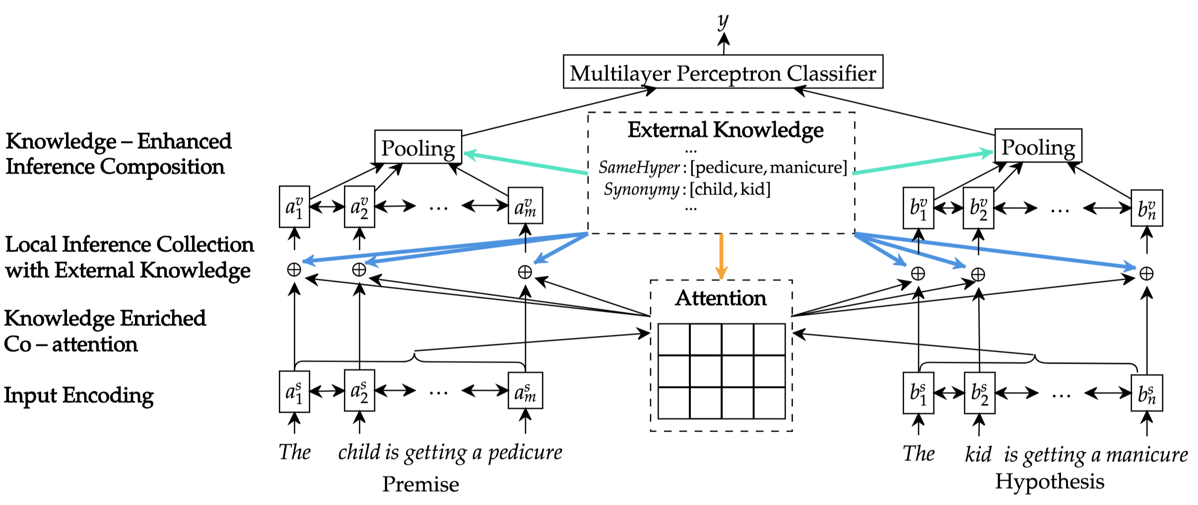
Figure 1: A high-level view of neural-network-based NLI models enriched with external knowledge in co-attention, local inference collection, and inference composition.

3.2 Encoding Premise and Hypothesis

Same as much previous work (Chen et al., 2017a, b), we encode the premise and the hypothesis with bidirectional LSTMs (BiLSTMs). The premise is represented as $\bm{a}=(a_{1},\dots,a_{m})$ and the hypothesis is $\bm{b}=(b_{1},\dots,b_{n})$, where $m$ and $n$ are the lengths of the sentences. Then $\bm{a}$ and $\bm{b}$ are embedded into $d_{e}$-dimensional vectors $[{\bf{E}}(a_{1}),\dots,{\bf{E}}(a_{m})]$ and $[{\bf{E}}(b_{1}),\dots,{\bf{E}}(b_{n})]$ using the embedding matrix ${\bf{E}}\in\mathbb{R}^{d_{e}\times|V|}$, where $|V|$ is the vocabulary size and ${\bf{E}}$ can be initialized with the pre-trained word embedding. To represent words in its context, the premise and the hypothesis are fed into BiLSTM encoders (Hochreiter and Schmidhuber, 1997) to obtain context-dependent hidden states ${\bm{a}}^{s}$ and ${\bm{b}}^{s}$:

$${\bm{a}}^{s}_{i} =\mathrm{Encoder}({\bf{E}}(\bm{a}),i)\,,$$ (1)

$${\bm{b}}^{s}_{j} =\mathrm{Encoder}({\bf{E}}(\bm{b}),j)\,.$$ (2)

where $i$ and $j$ indicate the $i$-th word in the premise and the $j$-th word in the hypothesis, respectively.

3.3 Knowledge-Enriched Co-Attention

As discussed above, soft-alignment of word pairs between the premise and the hypothesis may benefit from knowledge-enriched co-attention mechanism. Given the relation features ${\bm{r}}_{ij}\in\mathbb{R}^{d_{r}}$ between the premise’s $i$-th word and the hypothesis’s $j$-th word derived from the external knowledge, the co-attention is calculated as:

$$e_{ij}=({\bm{a}}^{s}_{i})^{\mathrm{T}}{\bm{b}}^{s}_{j}+F({\bm{r}}_{ij})\,.$$ (3)

The function $F$ can be any non-linear or linear functions. In this paper, we use $F({\bm{r}}_{ij})=\lambda\mathds{1}({\bm{r}}_{ij})$, where $\lambda$ is a hyper-parameter tuned on the development set and $\mathds{1}$ is the indication function as follows:

$$\mathds{1}({\bm{r}}_{ij})=\begin{cases}1&\quad\text{if }{\bm{r}}_{ij}\text{ is not a zero vector}\,;\\ 0&\quad\text{if }{\bm{r}}_{ij}\text{ is a zero vector}\,.\end{cases}$$ (4)

Intuitively, word pairs with semantic relationship, e.g., synonymy, antonymy, hypernymy, hyponymy and co-hyponyms, are probably aligned together. We will discuss how we construct external knowledge later in Section 4. We have also tried a two-layer MLP as a universal function approximator in function $F$ to learn the underlying combination function but did not observe further improvement over the best performance we obtained on the development datasets.

Soft-alignment is determined by the co-attention matrix ${\bf{e}}\in\mathbb{R}^{m\times n}$ computed in Equation (3), which is used to obtain the local relevance between the premise and the hypothesis. For the hidden state of the $i$-th word in the premise, i.e., ${\bm{a}}^{s}_{i}$ (already encoding the word itself and its context), the relevant semantics in the hypothesis is identified into a context vector ${\bm{a}}^{c}_{i}$ using $e_{ij}$, more specifically with Equation (5).

$$\alpha_{ij} =\frac{\exp(e_{ij})}{\sum_{k=1}^{n}\exp(e_{ik})}\,,~{}{\bm{a}}^{c}_{i}=\sum_{j=1}^{n}\alpha_{ij}{\bm{b}}^{s}_{j}\,,$$ (5)

$$\beta_{ij} =\frac{\exp(e_{ij})}{\sum_{k=1}^{m}\exp(e_{kj})}\,,~{}{\bm{b}}^{c}_{j}=\sum_{i=1}^{m}\beta_{ij}{\bm{a}}^{s}_{i}\,,$$ (6)

where ${\bm{\alpha}}\in\mathbb{R}^{m\times n}$ and ${\bm{\beta}}\in\mathbb{R}^{m\times n}$ are the normalized attention weight matrices with respect to the $2$-axis and $1$-axis. The same calculation is performed for each word in the hypothesis, i.e., ${\bm{b}}^{s}_{j}$, with Equation (6) to obtain the context vector ${\bm{b}}^{c}_{j}$.

3.4 Local Inference Collection with External Knowledge

By way of comparing the inference-related semantic relation between ${\bm{a}}_{i}^{s}$ (individual word representation in premise) and ${\bm{a}}_{i}^{c}$ (context representation from hypothesis which is align to word ${\bm{a}}^{s}_{i}$), we can model local inference (i.e., word-level inference) between aligned word pairs. Intuitively, for example, knowledge about hypernymy or hyponymy may help model entailment and knowledge about antonymy and co-hyponyms may help model contradiction. Through comparing ${\bm{a}}^{s}_{i}$ and ${\bm{a}}^{c}_{i}$, in addition to their relation from external knowledge, we can obtain word-level inference information for each word. The same calculation is performed for ${\bm{b}}_{j}^{s}$ and ${\bm{b}}_{j}^{c}$. Thus, we collect knowledge-enriched local inference information:

$${\bm{a}}^{m}_{i} =G([{\bm{a}}^{s}_{i};{\bm{a}}^{c}_{i};{\bm{a}}^{s}_{i}-{\bm{a}}^{c}_{i};{\bm{a}}^{s}_{i}\circ{\bm{a}}^{c}_{i};\sum_{j=1}^{n}\alpha_{ij}{\bm{r}}_{ij}])\,,$$ (7)

$${\bm{b}}^{m}_{j} =G([{\bm{b}}^{s}_{j},{\bm{b}}^{c}_{j};{\bm{b}}^{s}_{j}-{\bm{b}}^{c}_{j};{\bm{b}}^{s}_{j}\circ{\bm{b}}^{c}_{j};\sum_{i=1}^{m}\beta_{ij}{\bm{r}}_{ji}])\,,$$ (8)

where a heuristic matching trick with difference and element-wise product is used (Mou et al., 2016; Chen et al., 2017a). The last terms in Equation (7)(8) are used to obtain word-level inference information from external knowledge. Take Equation (7) as example, ${\bm{r}}_{ij}$ is the relation feature between the $i$-th word in the premise and the $j$-th word in the hypothesis, but we care more about semantic relation between aligned word pairs between the premise and the hypothesis. Thus, we use a soft-aligned version through the soft-alignment weight $\alpha_{ij}$. For the $i$-th word in the premise, the last term in Equation (7) is a word-level inference information based on external knowledge between the $i$-th word and the aligned word. The same calculation for hypothesis is performed in Equation (8). $G$ is a non-linear mapping function to reduce dimensionality. Specifically, we use a 1-layer feed-forward neural network with the ReLU activation function with a shortcut connection, i.e., concatenate the hidden states after ReLU with the input $\sum_{j=1}^{n}\alpha_{ij}{\bm{r}}_{ij}$ (or $\sum_{i=1}^{m}\beta_{ij}{\bm{r}}_{ji}$) as the output ${\bm{a}}^{m}_{i}$ (or ${\bm{b}}^{m}_{j}$).

3.5 Knowledge-Enhanced Inference Composition

In this component, we introduce knowledge-enriched inference composition. To determine the overall inference relationship between the premise and the hypothesis, we need to explore a composition layer to compose the local inference vectors (${\bm{a}}^{m}$ and ${\bm{b}}^{m}$) collected above:

$${\bm{a}}^{v}_{i} =\mathrm{Composition}({\bm{a}}^{m},i)\,,$$ (9)

$${\bm{b}}^{v}_{j} =\mathrm{Composition}({\bm{b}}^{m},j)\,.$$ (10)

Here, we also use BiLSTMs as building blocks for the composition layer, but the responsibility of BiLSTMs in the inference composition layer is completely different from that in the input encoding layer. The BiLSTMs here read local inference vectors (${\bm{a}}^{m}$ and ${\bm{b}}^{m}$) and learn to judge the types of local inference relationship and distinguish crucial local inference vectors for overall sentence-level inference relationship. Intuitively, the final prediction is likely to depend on word pairs appearing in external knowledge that have some semantic relation. Our inference model converts the output hidden vectors of BiLSTMs to the fixed-length vector with pooling operations and puts it into the final classifier to determine the overall inference class. Particularly, in addition to using mean pooling and max pooling similarly to ESIM (Chen et al., 2017a), we propose to use weighted pooling based on external knowledge to obtain a fixed-length vector as in Equation (11)(12).

$${\bm{a}}^{\mathrm{w}} =\sum_{i=1}^{m}\frac{\exp(H(\sum_{j=1}^{n}\alpha_{ij}{\bm{r}}_{ij}))}{\sum_{i=1}^{m}\exp(H(\sum_{j=1}^{n}\alpha_{ij}{\bm{r}}_{ij}))}{\bm{a}}^{v}_{i}\,,$$ (11)

$${\bm{b}}^{\mathrm{w}} =\sum_{j=1}^{n}\frac{\exp(H(\sum_{i=1}^{m}\beta_{ij}{\bm{r}}_{ji}))}{\sum_{j=1}^{n}\exp(H(\sum_{i=1}^{m}\beta_{ij}{\bm{r}}_{ji}))}{\bm{b}}^{v}_{j}\,.$$ (12)

In our experiments, we regard the function $H$ as a 1-layer feed-forward neural network with ReLU activation function. We concatenate all pooling vectors, i.e., mean, max, and weighted pooling, into the fixed-length vector and then put the vector into the final multilayer perceptron (MLP) classifier. The MLP has one hidden layer with tanh activation and softmax output layer in our experiments. The entire model is trained end-to-end, through minimizing the cross-entropy loss.

4 Experiment Set-Up

4.1 Representation of External Knowledge

Lexical Semantic Relations

As described in Section 3.1, to incorporate external knowledge (as a knowledge vector ${\bm{r}}_{ij}$) to the state-of-the-art neural network-based NLI models, we first explore semantic relations in WordNet (Miller, 1995), motivated by MacCartney (2009). Specifically, the relations of lexical pairs are derived as described in 1-4 below. Instead of using Jiang-Conrath WordNet distance metric (Jiang and Conrath, 1997), which does not improve the performance of our models on the development sets, we add a new feature, i.e., co-hyponyms, which consistently benefit our models.

1. Synonymy: It takes the value $1$ if the words in the pair are synonyms in WordNet (i.e., belong to the same synset), and $0$ otherwise. For example, [felicitous, good] = $1$, [dog, wolf] = $0$.

2. Antonymy: It takes the value $1$ if the words in the pair are antonyms in WordNet, and $0$ otherwise. For example, [wet, dry] = $1$.

3. Hypernymy: It takes the value $1-n/8$ if one word is a (direct or indirect) hypernym of the other word in WordNet, where $n$ is the number of edges between the two words in hierarchies, and $0$ otherwise. Note that we ignore pairs in the hierarchy which have more than 8 edges in between. For example, [dog, canid] = $0.875$, [wolf, canid] = $0.875$, [dog, carnivore] = $0.75$, [canid, dog] = $0$

4. Hyponymy: It is simply the inverse of the hypernymy feature. For example, [canid, dog] = $0.875$, [dog, canid] = $0$.

5. Co-hyponyms: It takes the value $1$ if the two words have the same hypernym but they do not belong to the same synset, and $0$ otherwise. For example, [dog, wolf] = $1$.

As discussed above, we expect features like synonymy, antonymy, hypernymy, hyponymy and co-hyponyms would help model co-attention alignment between the premise and the hypothesis. Knowledge of hypernymy and hyponymy may help capture entailment; knowledge of antonymy and co-hyponyms may help model contradiction. Their final contributions will be learned in end-to-end model training. We regard the vector ${\bm{r}}\in\mathbb{R}^{d_{r}}$ as the relation feature derived from external knowledge, where $d_{r}$ is $5$ here. In addition, Table 1 reports some key statistics of these features.

Feature	#Words	#Pairs
Synonymy	84,487	237,937
Antonymy	6,161	6,617
Hypernymy	57,475	753,086
Hyponymy	57,475	753,086
Co-hyponyms	53,281	3,674,700

Table 1: Statistics of lexical relation features.

In addition to the above relations, we also use more relation features in WordNet, including instance, instance of, same instance, entailment, member meronym, member holonym, substance meronym, substance holonym, part meronym, part holonym, summing up to 15 features, but these additional features do not bring further improvement on the development dataset, as also discussed in Section  5.

Relation Embeddings

In the most recent years graph embedding has been widely employed to learn representation for vertexes and their relations in a graph. In our work here, we also capture the relation between any two words in WordNet through relation embedding. Specifically, we employed TransE (Bordes et al., 2013), a widely used graph embedding methods, to capture relation embedding between any two words. We used two typical approaches to obtaining the relation embedding. The first directly uses 18 relation embeddings pretrained on the WN18 dataset (Bordes et al., 2013). Specifically, if a word pair has a certain type relation, we take the corresponding relation embedding. Sometimes, if a word pair has multiple relations among the 18 types; we take an average of the relation embedding. The second approach uses TransE’s word embedding (trained on WordNet) to obtain relation embedding, through the objective function used in TransE, i.e., ${\bm{l}}\approx{\bm{t}}-{\bm{h}}$, where ${\bm{l}}$ indicates relation embedding, ${\bm{t}}$ indicates tail entity embedding, and ${\bm{h}}$ indicates head entity embedding.

Note that in addition to relation embedding trained on WordNet, other relational embedding resources exist; e.g., that trained on Freebase (WikiData) (Bollacker et al., 2007), but such knowledge resources are mainly about facts (e.g., relationship between Bill Gates and Microsoft) and are less for commonsense knowledge used in general natural language inference (e.g., the color yellow potentially contradicts red).

4.2 NLI Datasets

In our experiments, we use Stanford Natural Language Inference (SNLI) dataset (Bowman et al., 2015) and Multi-Genre Natural Language Inference (MultiNLI) (Williams et al., 2017) dataset, which focus on three basic relations between a premise and a potential hypothesis: the premise entails the hypothesis (entailment), they contradict each other (contradiction), or they are not related (neutral). We use the same data split as in previous work  (Bowman et al., 2015; Williams et al., 2017) and classification accuracy as the evaluation metric. In addition, we test our models (trained on the SNLI training set) on a new test set (Glockner et al., 2018), which assesses the lexical inference abilities of NLI systems and consists of 8,193 samples. WordNet 3.0 (Miller, 1995) is used to extract semantic relation features between words. The words are lemmatized using Stanford CoreNLP 3.7.0 (Manning et al., 2014). The premise and the hypothesis sentences fed into the input encoding layer are tokenized.

4.3 Training Details

For duplicability, we release our code. All our models were strictly selected on the development set of the SNLI data and the in-domain development set of MultiNLI and were then tested on the corresponding test set. The main training details are as follows: the dimension of the hidden states of LSTMs and word embeddings are $300$. The word embeddings are initialized by 300D GloVe 840B (Pennington et al., 2014), and out-of-vocabulary words among them are initialized randomly. All word embeddings are updated during training. Adam (Kingma and Ba, 2014) is used for optimization with an initial learning rate of $0.0004$. The mini-batch size is set to $32$. Note that the above hyperparameter settings are same as those used in the baseline ESIM (Chen et al., 2017a) model. ESIM is a strong NLI baseline framework with the source code made available at https://github.com/lukecq1231/nli (the ESIM core code has also been adapted to summarization (Chen et al., 2016a) and question-answering tasks (Zhang et al., 2017a)).

The trade-off $\lambda$ for calculating co-attention in Equation (3) is selected in $[0.1,0.2,0.5,1,2,5,10,20,50]$ based on the development set. When training TransE for WordNet, relations are represented with vectors of $20$ dimension.

5 Experimental Results

5.1 Overall Performance

Table 2 shows the results of state-of-the-art models on the SNLI dataset. Among them, ESIM (Chen et al., 2017a) is one of the previous state-of-the-art systems with an 88.0% test-set accuracy. The proposed model, namely Knowledge-based Inference Model (KIM), which enriches ESIM with external knowledge, obtains an accuracy of 88.6%, the best single-model performance reported on the SNLI dataset. The difference between ESIM and KIM is statistically significant under the one-tailed paired $t$-test at the 99% significance level. Note that the KIM model reported here uses five semantic relations described in Section 4. In addition to that, we also use 15 semantic relation features, which does not bring additional gains in performance. These results highlight the effectiveness of the five semantic relations described in Section 4. To further investigate external knowledge, we add TransE relation embedding, and again no further improvement is observed on both the development and test sets when TransE relation embedding is used (concatenated) with the semantic relation vectors. We consider this is due to the fact that TransE embedding is not specifically sensitive to inference information; e.g., it does not model co-hyponyms features, and its potential benefit has already been covered by the semantic relation features used.

Model	Test
LSTM Att. (Rocktäschel et al., 2015)	83.5
DF-LSTMs (Liu et al., 2016a)	84.6
TC-LSTMs (Liu et al., 2016b)	85.1
Match-LSTM (Wang and Jiang, 2016)	86.1
LSTMN (Cheng et al., 2016)	86.3
Decomposable Att. (Parikh et al., 2016)	86.8
NTI (Yu and Munkhdalai, 2017b)	87.3
Re-read LSTM (Sha et al., 2016)	87.5
BiMPM (Wang et al., 2017)	87.5
DIIN (Gong et al., 2017)	88.0
BCN + CoVe (McCann et al., 2017)	88.1
CAFE (Tay et al., 2018)	88.5
ESIM (Chen et al., 2017a)	88.0
KIM (This paper)	88.6

Table 2: Accuracies of models on SNLI.

Table 3 shows the performance of models on the MultiNLI dataset. The baseline ESIM achieves 76.8% and 75.8% on in-domain and cross-domain test set, respectively. If we extend the ESIM with external knowledge, we achieve significant gains to 77.2% and 76.4% respectively. Again, the gains are consistent on SNLI and MultiNLI, and we expect they would be orthogonal to other factors when external knowledge is added into other state-of-the-art models.

Model	In	Cross
CBOW (Williams et al., 2017)	64.8	64.5
BiLSTM (Williams et al., 2017)	66.9	66.9
DiSAN (Shen et al., 2017)	71.0	71.4
Gated BiLSTM (Chen et al., 2017b)	73.5	73.6
SS BiLSTM (Nie and Bansal, 2017)	74.6	73.6
DIIN * (Gong et al., 2017)	77.8	78.8
CAFE (Tay et al., 2018)	78.7	77.9
ESIM (Chen et al., 2017a)	76.8	75.8
KIM (This paper)	77.2	76.4

Table 3: Accuracies of models on MultiNLI. * indicates models using extra SNLI training set.

5.2 Ablation Results

Figure 2 displays the ablation analysis of different components when using the external knowledge. To compare the effects of external knowledge under different training data scales, we randomly sample different ratios of the entire training set, i.e., 0.8%, 4%, 20% and 100%. “A” indicates adding external knowledge in calculating the co-attention matrix as in Equation (3), “I” indicates adding external knowledge in collecting local inference information as in Equation (7)(8), and “C” indicates adding external knowledge in composing inference as in Equation (11)(12). When we only have restricted training data, i.e., 0.8% training set (about 4,000 samples), the baseline ESIM has a poor accuracy of 62.4%. When we only add external knowledge in calculating co-attention (“A”), the accuracy increases to 66.6% (+ absolute 4.2%). When we only utilize external knowledge in collecting local inference information (“I”), the accuracy has a significant gain, to 70.3% (+ absolute 7.9%). When we only add external knowledge in inference composition (“C”), the accuracy gets a smaller gain to 63.4% (+ absolute 1.0%). The comparison indicates that “I” plays the most important role among the three components in using external knowledge. Moreover, when we compose the three components (“A,I,C”), we obtain the best result of 72.6% (+ absolute 10.2%). When we use more training data, i.e., 4%, 20%, 100% of the training set, only “I” achieves a significant gain, but “A” or “C” does not bring any significant improvement. The results indicate that external semantic knowledge only helps co-attention and composition when limited training data is limited, but always helps in collecting local inference information. Meanwhile, for less training data, $\lambda$ is usually set to a larger value. For example, the optimal $\lambda$ on the development set is $20$ for 0.8% training set, $2$ for the 4% training set, $1$ for the 20% training set and $0.2$ for the 100% training set.

Figure 3 displays the results of using different ratios of external knowledge (randomly keep different percentages of whole lexical semantic relations) under different sizes of training data. Note that here we only use external knowledge in collecting local inference information as it always works well for different scale of the training set. Better accuracies are achieved when using more external knowledge. Especially under the condition of restricted training data (0.8%), the model obtains a large gain when using more than half of external knowledge.

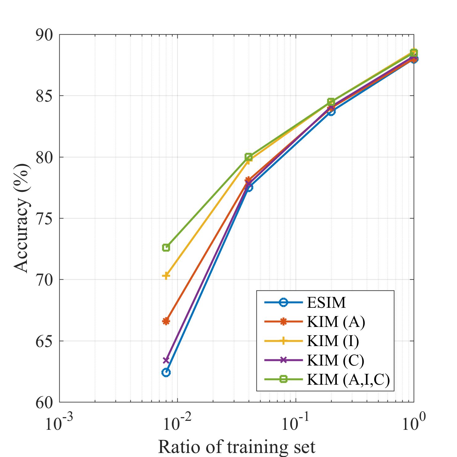
Figure 2: Accuracies of models of incorporating external knowledge into different NLI components, under different sizes of training data (0.8%, 4%, 20%, and the entire training data).

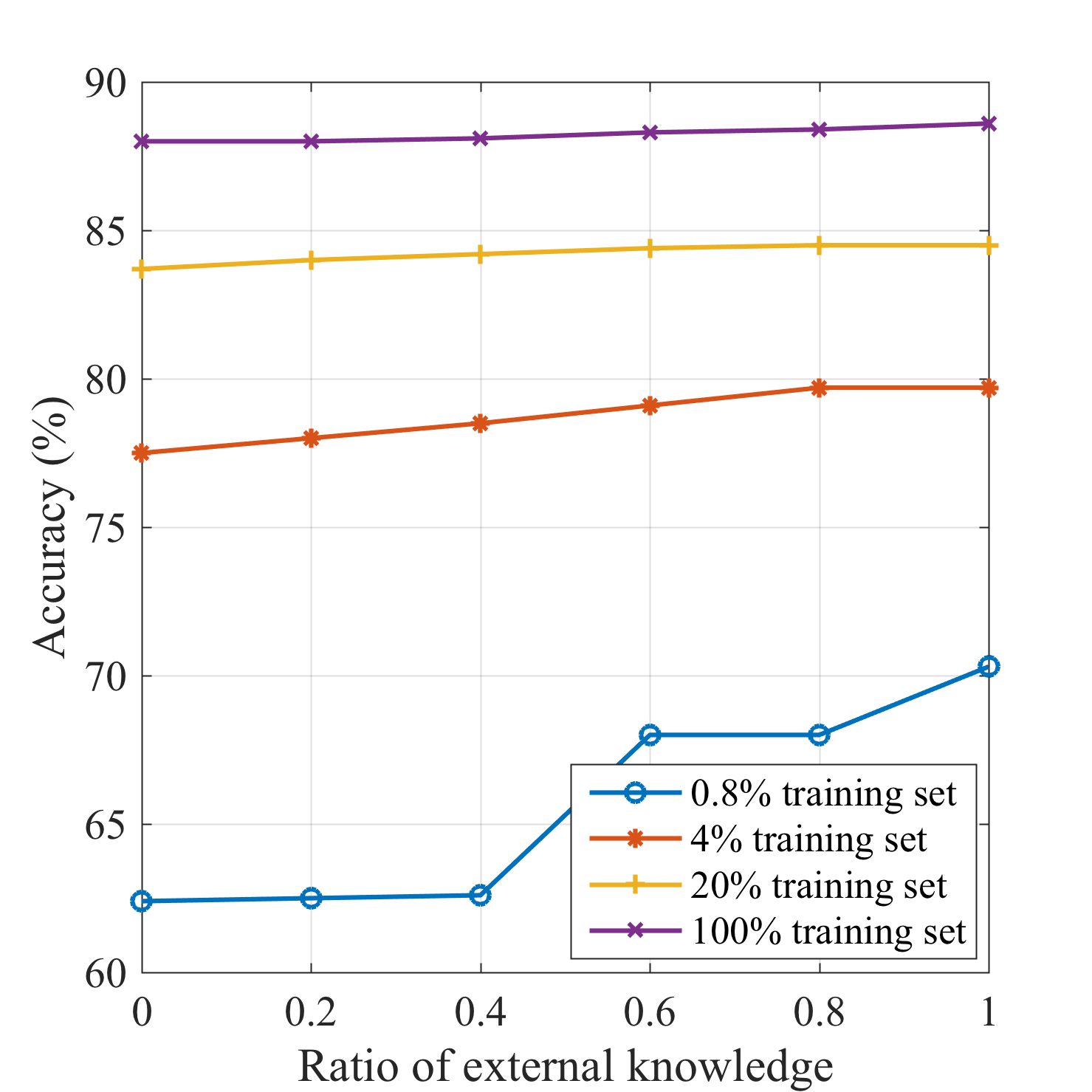
Figure 3: Accuracies of models under different sizes of external knowledge. More external knowledge corresponds to higher accuracies.

5.3 Analysis on the  (Glockner et al., 2018) Test Set

In addition, Table 4 shows the results on a newly published test set (Glockner et al., 2018). Compared with the performance on the SNLI test set, the performance of the three baseline models dropped substantially on the (Glockner et al., 2018) test set, with the differences ranging from 22.3% to 32.8% in accuracy. Instead, the proposed KIM achieves 83.5% on this test set (with only a 5.1% drop in performance), which demonstrates its better ability of utilizing lexical level inference and hence better generalizability.

Figure 5 displays the accuracy of ESIM and KIM in each replacement-word category of the (Glockner et al., 2018) test set. KIM outperforms ESIM in 13 out of 14 categories, and only performs worse on synonyms.

Model	SNLI	Glockner’s($\Delta$)
(Parikh et al., 2016)*	84.7	51.9 (-32.8)
(Nie and Bansal, 2017)*	86.0	62.2 (-23.8)
ESIM *	87.9	65.6 (-22.3)
KIM (This paper)	88.6	83.5 (  -5.1)

Table 4: Accuracies of models on the SNLI and  (Glockner et al., 2018) test set. * indicates the results taken from (Glockner et al., 2018).

Category	Instance	ESIM	KIM
Antonyms	1,147	70.4	86.5
Cardinals	759	75.5	93.4
Nationalities	755	35.9	73.5
Drinks	731	63.7	96.6
Antonyms WordNet	706	74.6	78.8
Colors	699	96.1	98.3
Ordinals	663	21.0	56.6
Countries	613	25.4	70.8
Rooms	595	69.4	77.6
Materials	397	89.7	98.7
Vegetables	109	31.2	79.8
Instruments	65	90.8	96.9
Planets	60	3.3	5.0
Synonyms	894	99.7	92.1
Overall	8,193	65.6	83.5

Table 5: The number of instances and accuracy per category achieved by ESIM and KIM on the (Glockner et al., 2018) test set.

5.4 Analysis by Inference Categories

We perform more analysis (Table 6) using the supplementary annotations provided by the MultiNLI dataset (Williams et al., 2017), which have 495 samples (about 1/20 of the entire development set) for both in-domain and out-domain set. We compare against the model outputs of the ESIM model across 13 categories of inference. Table 6 reports the results. We can see that KIM outperforms ESIM on overall accuracies on both in-domain and cross-domain subset of development set. KIM outperforms or equals ESIM in 10 out of 13 categories on the cross-domain setting, while only 7 out of 13 categories on in-domain setting. It indicates that external knowledge helps more in cross-domain setting. Especially, for antonym category in cross-domain set, KIM outperform ESIM significantly (+ absolute 5.0%) as expected, because antonym feature captured by external knowledge would help unseen cross-domain samples.

Category	In-domain		Cross-domain
	ESIM	KIM	ESIM	KIM
Active/Passive	93.3	93.3	100.0	100.0
Antonym	76.5	76.5	70.0	75.0
Belief	72.7	75.8	75.9	79.3
Conditional	65.2	65.2	61.5	69.2
Coreference	80.0	76.7	75.9	75.9
Long sentence	82.8	78.8	69.7	73.4
Modal	80.6	79.9	77.0	80.2
Negation	76.7	79.8	73.1	71.2
Paraphrase	84.0	72.0	86.5	89.2
Quantity/Time	66.7	66.7	56.4	59.0
Quantifier	79.2	78.4	73.6	77.1
Tense	74.5	78.4	72.2	66.7
Word overlap	89.3	85.7	83.8	81.1
Overall	77.1	77.9	76.7	77.4

Table 6: Detailed Analysis on MultiNLI.

5.5 Case Study

Table 7 includes some examples from the SNLI test set, where KIM successfully predicts the inference relation and ESIM fails. In the first example, the premise is “An African person standing in a wheat field” and the hypothesis “A person standing in a corn field”. As the KIM model knows that “wheat” and “corn” are both a kind of cereal, i.e, the co-hyponyms relationship in our relation features, KIM therefore predicts the premise contradicts the hypothesis. However, the baseline ESIM cannot learn the relationship between “wheat” and “corn” effectively due to lack of enough samples in the training sets. With the help of external knowledge, i.e., “wheat” and “corn” having the same hypernym “cereal”, KIM predicts contradiction correctly.

P/G	Sentences
e/c	p: An African person standing in a wheat field.
	h: A person standing in a corn field.
e/c	p: Little girl is flipping an omelet in the kitchen.
	h: A young girl cooks pancakes.
c/e	p: A middle eastern marketplace.
	h: A middle easten store.
c/e	p: Two boys are swimming with boogie boards.
	h: Two boys are swimming with their floats.

Table 7: Examples. Word in bold are key words in making final prediction. P indicates a predicted label and G indicates gold-standard label. e and c denote entailment and contradiction, respectively.

6 Conclusions

Our neural-network-based model for natural language inference with external knowledge, namely KIM, achieves the state-of-the-art accuracies. The model is equipped with external knowledge in its main components, specifically, in calculating co-attention, collecting local inference, and composing inference. We provide detailed analyses on our model and results. The proposed model of infusing neural networks with external knowledge may also help shed some light on tasks other than NLI.

References

- Ahn et al. (2016) Sungjin Ahn, Heeyoul Choi, Tanel Pärnamaa, and Yoshua Bengio. 2016. A neural knowledge language model. CoRR, abs/1608.00318.
- Bollacker et al. (2007) Kurt D. Bollacker, Robert P. Cook, and Patrick Tufts. 2007. Freebase: A shared database of structured general human knowledge. In Proceedings of the Twenty-Second AAAI Conference on Artificial Intelligence, July 22-26, 2007, Vancouver, British Columbia, Canada, pages 1962–1963.
- Bordes et al. (2013) Antoine Bordes, Nicolas Usunier, Alberto García-Durán, Jason Weston, and Oksana Yakhnenko. 2013. Translating embeddings for modeling multi-relational data. In Advances in Neural Information Processing Systems 26: 27th Annual Conference on Neural Information Processing Systems 2013. Proceedings of a meeting held December 5-8, 2013, Lake Tahoe, Nevada, United States., pages 2787–2795.
- Bowman et al. (2015) Samuel R. Bowman, Gabor Angeli, Christopher Potts, and Christopher D. Manning. 2015. A large annotated corpus for learning natural language inference. In Proceedings of the 2015 Conference on Empirical Methods in Natural Language Processing, EMNLP 2015, Lisbon, Portugal, September 17-21, 2015, pages 632–642.
- Bowman et al. (2016) Samuel R. Bowman, Jon Gauthier, Abhinav Rastogi, Raghav Gupta, Christopher D. Manning, and Christopher Potts. 2016. A fast unified model for parsing and sentence understanding. In Proceedings of the 54th Annual Meeting of the Association for Computational Linguistics, ACL 2016, August 7-12, 2016, Berlin, Germany, Volume 1: Long Papers.
- Bromley et al. (1993) Jane Bromley, Isabelle Guyon, Yann LeCun, Eduard Säckinger, and Roopak Shah. 1993. Signature verification using a siamese time delay neural network. In Advances in Neural Information Processing Systems 6, [7th NIPS Conference, Denver, Colorado, USA, 1993], pages 737–744.
- Chen et al. (2016a) Qian Chen, Xiaodan Zhu, Zhen-Hua Ling, Si Wei, and Hui Jiang. 2016a. Distraction-based neural networks for modeling document. In Proceedings of the Twenty-Fifth International Joint Conference on Artificial Intelligence, IJCAI 2016, New York, NY, USA, 9-15 July 2016, pages 2754–2760.
- Chen et al. (2017a) Qian Chen, Xiaodan Zhu, Zhen-Hua Ling, Si Wei, Hui Jiang, and Diana Inkpen. 2017a. Enhanced LSTM for natural language inference. In Proceedings of the 55th Annual Meeting of the Association for Computational Linguistics, ACL 2017, Vancouver, Canada, July 30 - August 4, Volume 1: Long Papers, pages 1657–1668.
- Chen et al. (2017b) Qian Chen, Xiaodan Zhu, Zhen-Hua Ling, Si Wei, Hui Jiang, and Diana Inkpen. 2017b. Recurrent neural network-based sentence encoder with gated attention for natural language inference. In Proceedings of the 2nd Workshop on Evaluating Vector Space Representations for NLP, RepEval@EMNLP 2017, Copenhagen, Denmark, September 8, 2017, pages 36–40.
- Chen et al. (2016b) Yun-Nung Chen, Dilek Z. Hakkani-Tür, Gökhan Tür, Asli Çelikyilmaz, Jianfeng Gao, and Li Deng. 2016b. Knowledge as a teacher: Knowledge-guided structural attention networks. CoRR, abs/1609.03286.
- Chen et al. (2015) Zhigang Chen, Wei Lin, Qian Chen, Xiaoping Chen, Si Wei, Hui Jiang, and Xiaodan Zhu. 2015. Revisiting word embedding for contrasting meaning. In Proceedings of the 53rd Annual Meeting of the Association for Computational Linguistics and the 7th International Joint Conference on Natural Language Processing of the Asian Federation of Natural Language Processing, ACL 2015, July 26-31, 2015, Beijing, China, Volume 1: Long Papers, pages 106–115.
- Cheng et al. (2016) Jianpeng Cheng, Li Dong, and Mirella Lapata. 2016. Long short-term memory-networks for machine reading. In Proceedings of the 2016 Conference on Empirical Methods in Natural Language Processing, EMNLP 2016, Austin, Texas, USA, November 1-4, 2016, pages 551–561.
- Choi et al. (2017) Jihun Choi, Kang Min Yoo, and Sang-goo Lee. 2017. Unsupervised learning of task-specific tree structures with tree-lstms. CoRR, abs/1707.02786.
- Conneau et al. (2017) Alexis Conneau, Douwe Kiela, Holger Schwenk, Loïc Barrault, and Antoine Bordes. 2017. Supervised learning of universal sentence representations from natural language inference data. In Proceedings of the 2017 Conference on Empirical Methods in Natural Language Processing, EMNLP 2017, Copenhagen, Denmark, September 9-11, 2017, pages 670–680.
- Dagan et al. (2005) Ido Dagan, Oren Glickman, and Bernardo Magnini. 2005. The PASCAL recognising textual entailment challenge. In Machine Learning Challenges, Evaluating Predictive Uncertainty, Visual Object Classification and Recognizing Textual Entailment, First PASCAL Machine Learning Challenges Workshop, MLCW 2005, Southampton, UK, April 11-13, 2005, Revised Selected Papers, pages 177–190.
- Faruqui et al. (2015) Manaal Faruqui, Jesse Dodge, Sujay Kumar Jauhar, Chris Dyer, Eduard H. Hovy, and Noah A. Smith. 2015. Retrofitting word vectors to semantic lexicons. In NAACL HLT 2015, The 2015 Conference of the North American Chapter of the Association for Computational Linguistics: Human Language Technologies, Denver, Colorado, USA, May 31 - June 5, 2015, pages 1606–1615.
- Glockner et al. (2018) Max Glockner, Vered Shwartz, and Yoav Goldberg. 2018. Breaking nli systems with sentences that require simple lexical inferences. In The 56th Annual Meeting of the Association for Computational Linguistics (ACL), Melbourne, Australia.
- Gong et al. (2017) Yichen Gong, Heng Luo, and Jian Zhang. 2017. Natural language inference over interaction space. CoRR, abs/1709.04348.
- Hochreiter and Schmidhuber (1997) Sepp Hochreiter and Jürgen Schmidhuber. 1997. Long short-term memory. Neural Computation, 9(8):1735–1780.
- Iftene and Balahur-Dobrescu (2007) Adrian Iftene and Alexandra Balahur-Dobrescu. 2007. Proceedings of the ACL-PASCAL Workshop on Textual Entailment and Paraphrasing, chapter Hypothesis Transformation and Semantic Variability Rules Used in Recognizing Textual Entailment. Association for Computational Linguistics.
- Jiang and Conrath (1997) Jay J. Jiang and David W. Conrath. 1997. Semantic similarity based on corpus statistics and lexical taxonomy. In Proceedings of the 10th Research on Computational Linguistics International Conference, ROCLING 1997, Taipei, Taiwan, August 1997, pages 19–33.
- Jijkoun and de Rijke (2005) Valentin Jijkoun and Maarten de Rijke. 2005. Recognizing textual entailment using lexical similarity. In Proceedings of the PASCAL Challenges Workshop on Recognising Textual Entailment.
- Kingma and Ba (2014) Diederik P. Kingma and Jimmy Ba. 2014. Adam: A method for stochastic optimization. CoRR, abs/1412.6980.
- Lin et al. (2017) Zhouhan Lin, Minwei Feng, Cícero Nogueira dos Santos, Mo Yu, Bing Xiang, Bowen Zhou, and Yoshua Bengio. 2017. A structured self-attentive sentence embedding. CoRR, abs/1703.03130.
- Liu et al. (2016a) Pengfei Liu, Xipeng Qiu, Jifan Chen, and Xuanjing Huang. 2016a. Deep fusion lstms for text semantic matching. In Proceedings of the 54th Annual Meeting of the Association for Computational Linguistics, ACL 2016, August 7-12, 2016, Berlin, Germany, Volume 1: Long Papers.
- Liu et al. (2016b) Pengfei Liu, Xipeng Qiu, Yaqian Zhou, Jifan Chen, and Xuanjing Huang. 2016b. Modelling interaction of sentence pair with coupled-lstms. In Proceedings of the 2016 Conference on Empirical Methods in Natural Language Processing, EMNLP 2016, Austin, Texas, USA, November 1-4, 2016, pages 1703–1712.
- Liu et al. (2015) Quan Liu, Hui Jiang, Si Wei, Zhen-Hua Ling, and Yu Hu. 2015. Learning semantic word embeddings based on ordinal knowledge constraints. In Proceedings of the 53rd Annual Meeting of the Association for Computational Linguistics and the 7th International Joint Conference on Natural Language Processing of the Asian Federation of Natural Language Processing, ACL 2015, July 26-31, 2015, Beijing, China, Volume 1: Long Papers, pages 1501–1511.
- Liu et al. (2016c) Yang Liu, Chengjie Sun, Lei Lin, and Xiaolong Wang. 2016c. Learning natural language inference using bidirectional LSTM model and inner-attention. CoRR, abs/1605.09090.
- MacCartney (2009) Bill MacCartney. 2009. Natural Language Inference. Ph.D. thesis, Stanford University.
- MacCartney et al. (2008) Bill MacCartney, Michel Galley, and Christopher D. Manning. 2008. A phrase-based alignment model for natural language inference. In 2008 Conference on Empirical Methods in Natural Language Processing, EMNLP 2008, Proceedings of the Conference, 25-27 October 2008, Honolulu, Hawaii, USA, A meeting of SIGDAT, a Special Interest Group of the ACL, pages 802–811.
- Manning et al. (2014) Christopher D. Manning, Mihai Surdeanu, John Bauer, Jenny Rose Finkel, Steven Bethard, and David McClosky. 2014. The stanford corenlp natural language processing toolkit. In Proceedings of the 52nd Annual Meeting of the Association for Computational Linguistics, ACL 2014, June 22-27, 2014, Baltimore, MD, USA, System Demonstrations, pages 55–60.
- McCann et al. (2017) Bryan McCann, James Bradbury, Caiming Xiong, and Richard Socher. 2017. Learned in translation: Contextualized word vectors. In Advances in Neural Information Processing Systems 30: Annual Conference on Neural Information Processing Systems 2017, 4-9 December 2017, Long Beach, CA, USA, pages 6297–6308.
- Miller (1995) George A. Miller. 1995. Wordnet: A lexical database for english. Commun. ACM, 38(11):39–41.
- Mou et al. (2016) Lili Mou, Rui Men, Ge Li, Yan Xu, Lu Zhang, Rui Yan, and Zhi Jin. 2016. Natural language inference by tree-based convolution and heuristic matching. In Proceedings of the 54th Annual Meeting of the Association for Computational Linguistics, ACL 2016, August 7-12, 2016, Berlin, Germany, Volume 2: Short Papers.
- Mrksic et al. (2017) Nikola Mrksic, Ivan Vulic, Diarmuid Ó Séaghdha, Ira Leviant, Roi Reichart, Milica Gasic, Anna Korhonen, and Steve J. Young. 2017. Semantic specialisation of distributional word vector spaces using monolingual and cross-lingual constraints. CoRR, abs/1706.00374.
- Nie and Bansal (2017) Yixin Nie and Mohit Bansal. 2017. Shortcut-stacked sentence encoders for multi-domain inference. In Proceedings of the 2nd Workshop on Evaluating Vector Space Representations for NLP, RepEval@EMNLP 2017, Copenhagen, Denmark, September 8, 2017, pages 41–45.
- Parikh et al. (2016) Ankur P. Parikh, Oscar Täckström, Dipanjan Das, and Jakob Uszkoreit. 2016. A decomposable attention model for natural language inference. In Proceedings of the 2016 Conference on Empirical Methods in Natural Language Processing, EMNLP 2016, Austin, Texas, USA, November 1-4, 2016, pages 2249–2255.
- Pennington et al. (2014) Jeffrey Pennington, Richard Socher, and Christopher D. Manning. 2014. Glove: Global vectors for word representation. In Proceedings of the 2014 Conference on Empirical Methods in Natural Language Processing, EMNLP 2014, October 25-29, 2014, Doha, Qatar, A meeting of SIGDAT, a Special Interest Group of the ACL, pages 1532–1543.
- Rocktäschel et al. (2015) Tim Rocktäschel, Edward Grefenstette, Karl Moritz Hermann, Tomás Kociský, and Phil Blunsom. 2015. Reasoning about entailment with neural attention. CoRR, abs/1509.06664.
- Sha et al. (2016) Lei Sha, Baobao Chang, Zhifang Sui, and Sujian Li. 2016. Reading and thinking: Re-read LSTM unit for textual entailment recognition. In COLING 2016, 26th International Conference on Computational Linguistics, Proceedings of the Conference: Technical Papers, December 11-16, 2016, Osaka, Japan, pages 2870–2879.
- Shen et al. (2017) Tao Shen, Tianyi Zhou, Guodong Long, Jing Jiang, Shirui Pan, and Chengqi Zhang. 2017. Disan: Directional self-attention network for rnn/cnn-free language understanding. CoRR, abs/1709.04696.
- Shen et al. (2018) Tao Shen, Tianyi Zhou, Guodong Long, Jing Jiang, Sen Wang, and Chengqi Zhang. 2018. Reinforced self-attention network: a hybrid of hard and soft attention for sequence modeling. CoRR, abs/1801.10296.
- Shi et al. (2016) Chen Shi, Shujie Liu, Shuo Ren, Shi Feng, Mu Li, Ming Zhou, Xu Sun, and Houfeng Wang. 2016. Knowledge-based semantic embedding for machine translation. In Proceedings of the 54th Annual Meeting of the Association for Computational Linguistics, ACL 2016, August 7-12, 2016, Berlin, Germany, Volume 1: Long Papers.
- Tay et al. (2018) Yi Tay, Luu Anh Tuan, and Siu Cheung Hui. 2018. A compare-propagate architecture with alignment factorization for natural language inference. CoRR, abs/1801.00102.
- Vendrov et al. (2015) Ivan Vendrov, Ryan Kiros, Sanja Fidler, and Raquel Urtasun. 2015. Order-embeddings of images and language. CoRR, abs/1511.06361.
- Wang and Jiang (2016) Shuohang Wang and Jing Jiang. 2016. Learning natural language inference with LSTM. In NAACL HLT 2016, The 2016 Conference of the North American Chapter of the Association for Computational Linguistics: Human Language Technologies, San Diego California, USA, June 12-17, 2016, pages 1442–1451.
- Wang et al. (2017) Zhiguo Wang, Wael Hamza, and Radu Florian. 2017. Bilateral multi-perspective matching for natural language sentences. In Proceedings of the Twenty-Sixth International Joint Conference on Artificial Intelligence, IJCAI 2017, Melbourne, Australia, August 19-25, 2017, pages 4144–4150.
- Wieting et al. (2015) John Wieting, Mohit Bansal, Kevin Gimpel, and Karen Livescu. 2015. From paraphrase database to compositional paraphrase model and back. TACL, 3:345–358.
- Williams et al. (2017) Adina Williams, Nikita Nangia, and Samuel R. Bowman. 2017. A broad-coverage challenge corpus for sentence understanding through inference. CoRR, abs/1704.05426.
- Yu and Munkhdalai (2017a) Hong Yu and Tsendsuren Munkhdalai. 2017a. Neural semantic encoders. In Proceedings of the 15th Conference of the European Chapter of the Association for Computational Linguistics, EACL 2017, Valencia, Spain, April 3-7, 2017, Volume 1: Long Papers, pages 397–407.
- Yu and Munkhdalai (2017b) Hong Yu and Tsendsuren Munkhdalai. 2017b. Neural tree indexers for text understanding. In Proceedings of the 15th Conference of the European Chapter of the Association for Computational Linguistics, EACL 2017, Valencia, Spain, April 3-7, 2017, Volume 1: Long Papers, pages 11–21.
- Zhang et al. (2017a) Junbei Zhang, Xiaodan Zhu, Qian Chen, Lirong Dai, Si Wei, and Hui Jiang. 2017a. Exploring question understanding and adaptation in neural-network-based question answering. CoRR, abs/arXiv:1703.04617v2.
- Zhang et al. (2017b) Shiyue Zhang, Gulnigar Mahmut, Dong Wang, and Askar Hamdulla. 2017b. Memory-augmented chinese-uyghur neural machine translation. In 2017 Asia-Pacific Signal and Information Processing Association Annual Summit and Conference, APSIPA ASC 2017, Kuala Lumpur, Malaysia, December 12-15, 2017, pages 1092–1096.