On the mass and decay constant of the P-wave ground and radially excited $h_{c}$ and $h_{b}$ axial-vector mesons

Abstract

The mass and decay constant of the heavy quarkonia $h_{Q}(1P)$ and $h_{Q}(2P)$ (Q = b, c) with quantum numbers $J^{PC}=1^{+-}$ are calculated in the framework of the two-point QCD sum rule method by taking into account the vacuum condensates up to eight dimensions. We compare our results for parameters of the $h_{b}(1P)$ and $h_{c}(1P)$ quarkonia, and their first radially excited states $h_{b}(2P)$ and $h_{c}(2P)$ with available experimental data as well as predictions of other theoretical studies existing in the literature. The results of present work may shed light on experimental searches for the $h_{c}(2P)$ state.

I Introduction

It is well-known that the heavy quarkonia can take over the same inscription in probing the QCD as the hydrogen atom did in the atomic physics. The search for heavy flavor production especially the quarkonia has played a prominent role and offered an insight into the dynamics of the strong interaction. A reliable description of heavy quarkonium states is of great interest not only for understanding their internal organizations but for our knowledge of non-perturbative aspects of QCD. Research on bottomonium and charmonium states can provide constraints on models of quarkonium spectroscopy, as well (for more information on the importance of quarkonia see for instance Cho:1995 ; Satz:2005 ; Rapp:2008 ; Voloshin:2007 ; Beringer:2012 ; Brambilla:2010 ; Soto:2017 ; YWang:2017 ; DeMori:2017 ; Ebert:2005jj ).

The production mechanism of quarkonium states in the experiment has been challenging for a long time and has presented important disagreements with the theoretical predictions Eichten:1979 ; Cacciari:1999 ; Fulsom:2014iha . To overcome this problem physicists have come to the idea that there might be a new set of particles. As a result of these efforts many XYZ states have been discovered Aubert:2005rm ; Choi:2007wga ; Mizuk:2008 ; Krokovny:2013mka ; Vinodkumar:2012tzs ; D0:X5568 ; X3872disc . These states were then interpreted as new multiquark configurations not fitting to the standard quark model. These developments have expanded our knowledge on hadrons and triggered wide discussions ended up in a new research area. Yet, unfortunately no a complete theoretical model has been established that could have a global description of what has been observed. New surveys with more production and decay mechanisms and search for possible partners having similar configurations may provide us with useful knowledge on their internal structures, quark organizations and interactions Andronic:2015wma . There have been a lot of experimental attempts on the spectroscopy of the new states in vacuum by different collaborations such as CLEO, LHCb, Belle, BESIII, etc. The PANDA experiment at FAIR is planned to begin taking data in 2025 aiming to explore the properties of charmonium-like particles in details.

Despite the impressive developments in the experimental side, not all of theoretically predicted charmonium states have been found, and some $2P$ resonances in the charmonium sector, such as the $h_{c}(2P)$ state are not described well Eichten:2004 ; Barnes:2007 . A clear identification of the mass of $h_{c}(2P)$ meson would complete all charmonium states expected by quark models to fall below the $D\overline{D}$ threshold (see also Rosner:2011sj ).

The P-wave state $h_{c}(1P)$ has been confirmed frequently since its first detection in the $p\bar{p}$ collisions by the R704 collaboration R704exp . The FNAL E760 experiment looked for the $h_{c}$ in the reaction $p\bar{p}\rightarrow h_{c}\rightarrow\pi^{0}J/\psi\rightarrow e^{+}e^{-}$ and announced a statistically significant enhancement with $M_{h_{c}}=3526.2\pm 0.2\pm 0.2\mathrm{MeV}$ and $\Gamma_{h_{c}}\leq 1.1\mathrm{MeV}$ E760exp . The best clue for the $h_{c}(1P)$ came out from the CLEO collaboration when looking for the isospin violating transition $e^{+}e^{-}\rightarrow\Upsilon(2S)\rightarrow h_{c}\pi^{0}$ CleoRosner . The mass of $h_{c}(2^{1}P_{1})$ was estimated around ($3934-3956)\mathrm{MeV}$ via HISH Model Son . In 2016, the BESIII collaboration reported a very good $h_{c}$ signal in the reaction channels $h_{c}\rightarrow\gamma\eta^{\prime}$ and $h_{c}\rightarrow\gamma\eta$ with a statistical significance of $8.4\sigma$ and $4.0\sigma$, respectively BES3Ablikimradiative . Very recently two resonances were observed in the $e^{+}e^{-}\rightarrow\pi^{+}\pi^{-}h_{c}$ process located in the mass region between $4.2\mathrm{GeV/c^{2}}$ and $4.4\mathrm{GeV/c^{2}}$, where the vector charmonium hybrid states have been predicted by various QCD calculations Ablikimhibrit2017 .

As for the spin-singlet P-wave bottomonium state $h_{b}(1P)$, the BaBar collaboration first reported the evidence in the sequential process $\Upsilon(3S)\rightarrow\pi^{0}h_{b}(1P)\rightarrow\pi^{0}\gamma\eta_{b}(1S)$ in 2011 Lees:2011Babar . The resonance $h_{b}(1P)$ was investigated and detected later again by Belle in the transition $\Upsilon(5S)\rightarrow h_{b}(1P)\pi^{+}\pi^{-}$ Bondar:Belle2012 ; Adachi:Belle .

The P-wave singlet charmonium and bottonium systems can give precious clues on spin-spin (or hyperfine) interactions between quarks at which the complications due to the relativistic effects are less important compared to the light quark systems. The way of analyzing the spin-spin interactions between quarks is to introduce a central potential term. In a QCD-based potential model, the potential term is commonly described as a Coulomb term stemming from one-gluon exchange plus a confining term. Regarding this potential, the hyperfine splitting between the spin-singlet and spin-triplet P-wave states is very small Buchmuller:2012 .

For instance, the $Y(4260)$ resonance has been considered in literature as a hybrid with a color octet $c\bar{c}$ pair bound with a gluon. However, a new decay is observed, $Y(4260)\rightarrow h_{c}\pi^{+}\pi^{-}$ Ablikimhibrit2017 , which would imply a spin flip of the heavy quark system. If another measurement will confirm this production mechanism, the hybrid interpretation of the $Y(4260)$ state would be potently disregarded. A similar case is found in the decay channel $\Upsilon(10860)\rightarrow\Upsilon(1S,2S,3S)\pi^{+}\pi^{-}$ and $\Upsilon(10860)\rightarrow h_{b}(1P,2P)\pi^{+}\pi^{-}$. Meanwhile, discoveries of the two charged bottomonia states $Z^{+}_{b}(10610)$ and $Z^{+}_{b}(10650)$ Adachi:Belle , found in the decays $\Upsilon(10860)/Y_{b}\rightarrow Z^{+}_{b}(10610)\pi^{-},Z^{+}_{b}(10650)\pi^{-}$, yielding $\Upsilon(1S)\pi^{+}\pi^{-},\Upsilon(2S)\rightarrow\pi^{+}\pi^{-},\Upsilon(3S)\pi^{+}\pi^{-},h_{b}(1P)\pi^{+}\pi^{-}$ and $h_{b}(2P)\pi^{+}\pi^{-}$ final states, indicates a tetraquark interpretation. In the tetraquark picture, the two $Z_{b}$ states have both (spin-0) and (spin-1) components in Fock space. Finally decays of some exotica into $h_{b}$ and $h_{c}$ mesons is very crucial for determining their inner structures and dynamics AhmetAli2017 .

The mesons $h_{c}(1P)$ and $h_{b}(1P)$ have been previously investigated using different models such as Extended Potential Model Akbar:2015EPM , Nonrelativistic Quark Models Deng:2016QM , Friedrichs-model-like Scheme Zhou:2017FMLS , Relativistic Quark Model Bhat:2017RQM ; Souza:2017RQM , Quark Model Godfrey:1985dt , Screened potential Li:2009zu , Holography Inspired Stringy Hadron(HISH) Son and Lattice QCD Becirevic:2013bsa .

In the present work, we study the ground-state heavy quarkonia $h_{b}(1P)$ and $h_{c}(1P)$, and their first radially excited states $h_{b}(2P)$, and $h_{c}(2P)$ via the QCD sum rule method Shifman1 ; Shifman2 , and make predictions for their masses and decay constants. It is known that QCD sum rule is one of the powerful and effective non-perturbative methods that provide valuable information in the search for the excited quarkonium states and exotica. We compare also our results with available experimental data and relevant theoretical predictions presented in the literature.

The paper is arranged in the following way. In section II we briefly review the theoretical background for QCD sum rules and present details of the mass and decay constant calculations for hidden-charm and bottom states with $J^{PC}=1^{+-}$. In section III we discuss the results and compare our conclusions with ones obtained in the context of other models. Last section is devoted to the summary and outlook.

II Determination of Mass and Decay Constant of $h_{c}$ and $h_{b}$ States

The aim of QCD sum rule method is to extract the hadronic observables (e.g. masses, coupling constants etc.) from microscopic QCD degrees of freedom such as vacuum quark-gluon condensates and quark masses. This approach relates the micro world of QCD at high energies to the hadronic sector at low energies. The correlation function of two currents is introduced and treated by the help of the operator product expansion (OPE), where the short and long-distance effects are separated. The former is calculated with QCD perturbation theory, while the latter is parameterized in terms of the quark-gluon vacuum condensates.

The strategy behind this technique is to interpret an appropriate correlation function in two different ways. On one hand it is identified with a hadronic propagator, called Physical (or Phenomenological) side. On the other hand, as previously mentioned, the correlation function is calculated in terms of the quarks and gluons and their interactions with the QCD vacuum, called QCD (or Theoretical) side. Then, the result of the QCD calculations is matched to a sum over the hadronic states via a dispersion relation. The sum rules obtained allow one to calculate different observable characteristics of the hadronic ground and excited states. The interpolating currents representing the hadronic states in this approach couple not only to their ground states, but also to their excited states with the same quark contents and quantum numbers. Therefore, via this method, in addition to the parameters such as the mass and decay constant of the ground state $h_{Q}(1P)$, spectroscopic parameters of its first radial excitation, i.e. $h_{Q}(2P)$ can be calculated, as well.

In this section, we present the details of the calculation of the masses and decay constants of the $h_{b}(1P),h_{b}(2P),h_{c}(1P)$ and $h_{c}(2P)$ mesons with $J^{PC}=1^{+-}$. The starting point is to deal with the following two-point correlation function Shifman1 ; Shifman2 :

$$\Pi_{\mu\nu}(p)=i\int d^{4}x~{}e^{ip\cdot x}\langle 0|\mathcal{T}\{J_{\mu}^{h_{Q}}(x)J_{\nu}^{\dagger h_{Q}}(0)\}|0\rangle,$$ (1)

where $J_{\mu}(x)$ is the interpolating current with the quantum numbers $J^{PC}=1^{+-}$Reinders :

$$J_{\mu}^{h_{Q}}(x)=\bar{Q}_{i}(x)\vec{\partial}_{\mu}(x)\gamma_{5}{Q}_{i}(x),$$ (2)

where $Q=b$ or $c$, and $i$ is the color index.

Firstly, we determine the sum rules for the masses $m_{h_{Q}}$ and decay constants $f_{h_{Q}}$ of the ground states. The decay constant of a state represents the relation of the hadronic state with the vacuum through its interpolating current. This is the main input in analyses of the possible strong, electromagnetic and weak decays of hadrons in order to estimate their total width. To calculate the parameters of the ground states, we employ the “ground state + continuum” approximation. Later the “ground state +first excited state + continuum” approximation is used to derive sum rules for the $h_{b}(2P)$ and $h_{c}(2P)$ mesons. So the masses and decay constants of $h_{c}(2P)$ and $h_{b}(2P)$ can be extracted from these expressions. Obtained numerical values for the parameters of the ground states are used as inputs in the sum rules for the excited $h_{b}(2P)$ and $h_{c}(2P)$ mesons.

To obtain the physical side, a complete set of intermediate hadronic states with the same quantum numbers as the current operator $J_{\mu}(x)$ can be inserted into the correlation function. Then isolating the terms that we are interested in from other quarkonium states and carrying out the integration over $x$, we obtain the following expression:

$$\Pi_{\mu\nu}^{\mathrm{Phys.}}(p)=\frac{\langle 0|J_{\mu}^{h_{Q}(1P)}|h_{Q}(1P)\rangle\langle h_{Q}(1P)|J_{\nu}^{\dagger h_{Q}(1P)}|0\rangle}{m_{h_{Q}(1P)}^{2}-p^{2}}$$

$$+\frac{\langle 0|J_{\mu}^{h_{Q}(2P)}|h_{Q}(2P)\rangle\langle h_{Q}(2P)|J_{\nu}^{h_{Q}(2P)\dagger}|0\rangle}{m_{h_{Q}(2P)}^{2}-p^{2}}+\ldots,$$ (3)

where $m_{h_{Q}(1P)}$ and $m_{h_{Q}(2P)}$ are the masses of $h_{Q}(1P)$ and $h_{Q}(2P)$ states, respectively. The ellipsis in Eq. (3) represent contributions coming from higher resonances and continuum states.

To complete the calculations of the phenomenological side of the sum rules we introduce the matrix elements through masses and decay constants of $h_{Q}(1P)$ and $h_{Q}(2P)$ mesons as

$$\langle 0|J_{\mu}^{h_{Q}(1P)}|h_{Q}(1P)\rangle=f_{h_{Q}(1P)}m^{2}_{h_{Q}(1P)}\varepsilon_{\mu},$$

$$\langle 0|J_{\mu}^{h_{Q}(2P)}|h_{Q}(2P)\rangle=f_{h_{Q}(2P)}m^{2}_{h_{Q}(2P)}\tilde{\varepsilon}_{\mu}$$ (4)

where $\varepsilon_{\mu}$ and $\tilde{\varepsilon}_{\mu}$ are the polarization vectors of the $h_{Q}(1P)$ and $h_{Q}(2P)$ states, respectively. So the function $\Pi_{\mu\nu}^{\mathrm{Phys.}}(p)$ can be written as

$$\Pi_{\mu\nu}^{\mathrm{Phys.}}(p)=\frac{m_{h_{Q}(1P)}^{4}f_{h_{Q}(1P)}^{2}}{m_{h_{Q}(1P)}^{2}-p^{2}}\Bigg{(}-g_{\mu\nu}+\frac{p_{\mu}p_{\nu}}{m_{h_{Q}(1P)}^{2}}\Bigg{)}$$

$$+\frac{m_{h_{Q}(2P)}^{4}f_{h_{Q}(2P)}^{2}}{m_{h_{Q}(2P)}^{2}-p^{2}}\Bigg{(}-g_{\mu\nu}+\frac{p_{\mu}p_{\nu}}{m_{h_{Q}(2P)}^{2}}\Bigg{)}+\ldots.$$ (5)

Then Borel transformation applied to Eq. (5) yields

$$\mathcal{B}(p^{2})~{}\Pi_{\mu\nu}^{\mathrm{Phys.}}(p) = m_{h_{Q}(1P)}^{4}f_{h_{Q}(1P)}^{2}e^{-m_{h_{Q}(1P)}^{2}/{M}^{2}}$$ (6)

$$\times \left(-g_{\mu\nu}+\frac{p_{\mu}p_{\nu}}{m_{h_{Q}(1P)}^{2}}\right)$$

$$+ m_{h_{Q}(2P)}^{4}f_{h_{Q}(2P)}^{2}e^{-m_{h_{Q}(2P)}^{2}/{M}^{2}}$$

$$\times \left(-g_{\mu\nu}+\frac{p_{\mu}p_{\nu}}{m_{h_{Q}(2P)}^{2}}\right)+\ldots,$$

where $M^{2}$ is the Borel parameter that should be fixed.

The correlation function on QCD side, $\Pi_{\mu\nu}^{\mathrm{QCD}}(p)$, can be written down by contracting the heavy quark fields. After simple manipulations and putting $y=0$, it reads

$$\Pi_{\mu\nu}^{\mathrm{QCD}}(p) = i\int d^{4}x~{}e^{ip.x}$$

$$\times \mathrm{Tr}~{}[\vec{\partial}_{\mu}(x)\vec{\partial}_{\nu}(y){S}_{Q}^{ji}(y-x)\gamma_{5}S_{Q}^{ij}(x-y)\gamma_{5}]|_{y=0},$$

where the $S_{Q}^{ij}$ is the heavy quark propagator explicit form of which is presented below Reinders ;

$$S_{Q}^{ij}(x)=i\int\frac{d^{4}k}{(2\pi)^{4}}e^{-ikx}\Bigg{\{}\frac{\delta_{ij}\left({\not{k}}+m_{Q}\right)}{k^{2}-m_{Q}^{2}}$$

$$-\frac{g_{s}G_{ij}^{\alpha\beta}}{4}\frac{\sigma_{\alpha\beta}\left({\not{k}}+m_{Q}\right)+\left({\not{k}}+m_{Q}\right)\sigma_{\alpha\beta}}{(k^{2}-m_{Q}^{2})^{2}}$$

$$+\frac{g_{s}^{2}G^{2}}{12}~{}\delta_{ij}~{}m_{Q}\frac{k^{2}+m_{Q}{\not{k}}}{(k^{2}-m_{Q}^{2})^{4}}+\frac{g_{s}^{3}G^{3}}{48}~{}\delta_{ij}\frac{\left({\not{k}}+m_{Q}\right)}{(k^{2}-m_{Q}^{2})^{6}}$$

$$\times\left[{\not{k}}\left(k^{2}-3m_{Q}^{2}\right)+2m_{Q}\left(2k^{2}-m_{Q}^{2}\right)\right]\left({\not{k}}+m_{Q}\right)+...\Bigg{\}},$$

(8)

In Eq. (8) we used the following notations

$$G_{ij}^{\alpha\beta}=G_{A}^{\alpha\beta}t_{ij}^{A},\,\,~{}~{}G^{2}=G_{\alpha\beta}^{A}G_{\alpha\beta}^{A},$$

$$G^{3}=\,\,f^{ABC}G_{\mu\nu}^{A}G_{\nu\delta}^{B}G_{\delta\mu}^{C},$$ (9)

with $i,\,j=1,2,3$ being the color indices and $A,B,C=1,\,2\,\ldots 8$. In Eq. (9), $t^{A}=\lambda^{A}/2$, $\lambda^{A}$ are the Gell-Mann matrices and the gluon field strength tensor $G_{\alpha\beta}^{A}\equiv G_{\alpha\beta}^{A}(0)$ is fixed at $x=0$.

The function $\Pi_{\mu\nu}^{\mathrm{QCD}}(p)$ has two different structures, and can be expressed as a sum of two components as follows

$$\Pi_{\mu\nu}^{\mathrm{QCD}}(p)=\Pi^{\mathrm{QCD}}(p^{2})(-g_{\mu\nu})+\widetilde{\Pi}^{\mathrm{QCD}}(p^{2})p_{\mu}p_{\nu}.$$ (10)

The QCD sum rules for the physical quantities of $h_{Q}(2P)$ can be extracted after equating the coefficient of the same structures in both $\Pi_{\mu\nu}^{\mathrm{Phys}}(p)$ and $\Pi_{\mu\nu}^{\mathrm{QCD}}(p)$. To continue our evaluations, we select the structure $p_{\mu}p_{\nu}$. The invariant function $\widetilde{\Pi}^{\mathrm{QCD}}(p^{2})$ corresponding to this structure can be represented as the dispersion integral

$$\widetilde{\Pi}^{\mathrm{QCD}}(p^{2})=\int_{4m_{Q}^{2}}^{\infty}ds~{}\frac{\rho^{\mathrm{QCD}}(s)}{s-p^{2}}+\mathrm{subtracted~{}terms},$$ (11)

where $\rho^{\mathrm{QCD}}(s)$ is the corresponding two-point spectral density. It consists of two parts and can be expressed as

$$\rho^{\mathrm{QCD}}(s)=\rho^{\mathrm{Pert.}}(s)+\rho^{\mathrm{Nonpert.}}(s).$$ (12)

Here $\rho^{\mathrm{Pert.}}(s)$ is the perturbative part of the spectral density that is given by the formula

$$\rho^{\mathrm{Pert.}}(s)=\frac{1}{8\pi^{2}}(-12m_{Q}^{2}+3s).$$ (13)

The non-perturbative part of the spectral density is presented in the Appendix. After applying the Borel transformation on the variable $p^{2}$ to both the physical and QCD sides of the sum rules and subtraction of the contributions of the higher states and continuum using the quark-hadron duality assumption, we find the required sum rules. The sum rules for the mass and decay constant of the excited $h_{Q}(2P)$ states in terms of the parameters of the $h_{Q}(1P)$ mesons, are found as:

$$m^{2}_{h_{Q}(2P)}=\frac{\int_{4m_{Q}^{2}}^{s_{0}^{\star}}ds~{}\rho^{\mathrm{QCD}}(s)~{}s~{}e^{-s/M^{2}}-f_{h_{Q}(1P)}^{2}m_{h_{Q}(1P)}^{4}e^{-m_{h_{Q}(1P)}^{2}/M^{2}}}{\int_{4m_{h_{Q}}^{2}}^{s_{0}^{\star}}ds~{}\rho^{\mathrm{QCD}}(s)~{}e^{-s/M^{2}}-f_{h_{Q}(1P)}^{2}m_{h_{Q}(1P)}^{2}e^{-m_{h_{Q}(1P)}^{2}/M^{2}}},$$ (14)

and

$$f_{h_{Q}(2P)}^{2}=\frac{1}{m_{h_{Q}(2P)}^{2}}\Bigg{[}\int_{4m_{Q}^{2}}^{s_{0}^{\star}}ds~{}\rho^{\mathrm{QCD}}(s)~{}e^{\Big{(}m_{h_{Q}(2P)}^{2}-s\Big{)}/M^{2}}-f_{h_{Q}(1P)}^{2}m_{h_{Q}(1P)}^{2}e^{\Big{(}m_{h_{Q}(2P)}^{2}-m_{h_{Q}(1P)}^{2}\Big{)}/M^{2}}\Bigg{]}.$$ (15)

Here $s_{0}^{\star}$ is the continuum threshold parameter separating the contribution of the “$h_{Q}(1P)+h_{Q}(2P)$” states from the contribution due to “higher resonances and continuum”. As we previously mentioned the mass and decay constant of $h_{Q}(1P)$ enter into Eqs. (14) and (15) as the inputs. The mass of the $h_{Q}(1P)$ state can be extracted from the sum rule

$$m_{h_{Q}(1P)}^{2}=\frac{\int_{4m_{Q}^{2}}^{s_{0}}ds~{}\rho^{\mathrm{QCD}}(s)~{}s~{}e^{-s/M^{2}}}{\int_{4m_{Q}^{2}}^{s_{0}}ds~{}\rho^{\mathrm{QCD}}(s)~{}e^{-s/M^{2}}},$$ (16)

whereas to obtain the numerical value of the decay constant $f_{h_{Q}(1P)}$ we use the following expression

$$f_{h_{Q}(1P)}^{2}=\frac{1}{m_{h_{Q}(1P)}^{2}}\int_{4m_{Q}^{2}}^{s_{0}}ds~{}\rho^{\mathrm{QCD}}(s)e^{\Big{(}m_{h_{Q}(1P)}^{2}-s\Big{)}/M^{2}}.$$ (17)

In Eqs. (16) and (17) $s_{0}$ is the continuum threshold, which separates the contribution of the ground state $h_{Q}(1P)$ from those of the higher resonances and continuum. The sum rules for the ground and first radially excited states contain the same spectral density $\rho^{\mathrm{QCD}}(s)$, but the continuum threshold has to obey $s_{0}<s_{0}^{\star}$.

III Numerical Analysis

The sum rules obtained in this study allow us to calculate characteristics of the ground-state mesons and their first radial excitations. The obtained sum rules depend on the Borel mass parameter $M^{2}$ and continuum threshold $s_{0}$. Nevertheless, the dependence of physical quantities extracted from the sum rules on these auxiliary parameters should remain inside the standard limits, allowed by the method used, i. e. the uncertainties should not exceed the $30\%$ of the total values. These limits are determined by the systematic errors of the method coming from the quark-hadron duality assumption and those belong to the variations of the auxiliary parameters as well as other inputs. The sum rules found include the vacuum expectations of the different gluon operators as well as the heavy quark masses as input parameters, numerical values of which are presented in Table I.

Parameters	Values
$m_{c}$	$(1.67\pm 0.07)~{}\mathrm{GeV}$
$m_{b}$	$(4.78\pm 0.06)~{}\mathrm{GeV}$
$\langle\frac{\alpha_{s}G^{2}}{\pi}\rangle$	$(0.012\pm 0.004)~{}\mathrm{GeV}^{4}$
$\langle g_{s}^{3}G^{3}\rangle$	$(0.57\pm 0.29)~{}\mathrm{GeV}^{6}$

Table 1: Input parameters (see, Refs. Patrignani:2016xqp ; Shifman1 ; Shifman2 ; Ioffe:2005ym ; Belyaev:1982cd ).

Resonance	$h_{c}$	$h_{b}$
$M^{2}~{}(\mathrm{GeV}^{2}$)	$3-6$	$10-16$
$s_{0}~{}(\mathrm{GeV}^{2}$)	$13-15$	$100-104$
$s_{0}^{\star}~{}(\mathrm{GeV}^{2}$)	$16-18$	$107-111$

Table 2: Values of the Borel parameter and continuum thresholds used in this study to evaluate parameters of the $h_{c}$ and $h_{b}$ mesons.

The numerical analyses performed allow us to fix the working intervals of the parameters $M^{2}$ and $s_{0}$, where the standard conditions (pole dominance and OPE convergence) are satisfied. The upper bound on $M^{2}$ is found requiring that the contributions of the resonances under consideration exceed the contributions of the higher states and continuum. Its lower bound is found demanding the convergence of the OPE and exceeding the perturbative part over the total non-perturbative contributions. The parameters $s_{0}$ and $s_{0}^{*}$, are determined from the conditions that guarantee the sum rules to have the best stability in the allowed $M^{2}$ regions. This is possible by achieving the maximum pole contributions and the best convergence of the OPE. The obtained working region for the Borel parameter and continuum thresholds are presented in Table 2.

In figs. (1)- (4), we show the dependence of $m_{h_{Q}(1P)}$, $f_{h_{Q}(1P)}$, $m_{h_{Q}(2P)}$ and $f_{h_{Q}(2P)}$ on $M^{2}$ at fixed $s_{0}$, and as functions of $s_{0}$ for chosen values of $M^{2}$. The masses of the $h_{Q}$ mesons are rather stable with respect to the variations of the auxiliary parameters $M^{2}$ and $s_{0}^{(*)}$, compared to the decay constants $f_{h_{Q}}(1P,2P)$ which are relatively sensitive to the changes of the auxiliary parameters. The logic behind this is rather simple: the sum rules for the masses of the states under consideration are obtained as ratios of two integrals over the spectral densities $\rho(s)$ and $s\rho(s)$, which considerably decrease the effects due to the changes of the $M^{2}$ and $s_{0}$. On the contrary, the decay constants depend on the aforesaid integrals themselves, and therefore, undergone relatively sizable variations. Nevertheless, theoretical errors for $f_{h_{Q}(1P)}$ and $f_{h_{Q}(2P)}$ arising from uncertainties of $M^{2}$ and $s_{0}$, and other input parameters stay within the allowed intervals for the theoretical uncertainties ingrained in sum rule calculations which may reach to, as we previously mentioned, $30\%$ of the total values.

The numerical values extracted from the sum rules for the physical quantities are collected in Table 3, where we write down the masses of the mesons $h_{Q}(2P)$ and $h_{Q}(1P)$. The presented errors belong to the variations of the results with respect to the variations of the auxiliary parameters in their working region as well as those uncertainties coming from the other input parameters. We compare our predictions with the existing experimental data as well as other theoretical results. It is seen, that $m_{h_{c}(1P)}$, $m_{h_{b}(1P)}$ and $m_{h_{b}(2P)}$ are in agreement with the existing experimental data within the errors. The results of all theoretical studies on the masses of the states under consideration are roughly in agreements with each other within the uncertainties.

Our results for the decay constants of corresponding mesons compared to other theoretical predictions are presented in Table 4. We see overall considerable differences among different theoretical predictions on the decay constants of the states under consideration. Some predictions are consistent with each other within the errors. Even if we consider the errors of some theoretical predictions on the decay constants, however, the results differ up to a factor of two. The decay constants are the main inputs in the calculations of the total widths of the states under considerations via their possible strong, electromagnetic and weak decays. Further experimental data on the width and mass of the considered states are needed in order to determine which of the presented nonperturbative methods does work, well.

Parameter $[\mathrm{MeV}]$	$h_{c}(1P)$	$h_{c}(2P)$	$h_{b}(1P)$	$h_{b}(2P)$
$M_{\mathrm{Exp.}}$	$3525.38\pm 0.11$ Patrignani:2016xqp	-	$9899.3\pm 0.8$ Patrignani:2016xqp	$10259.8\pm 1.2$ Patrignani:2016xqp
$M_{\mathrm{Our~{}Work}}$	$3581^{+61}_{-60}$	$3897^{+68}_{-69}$	$9854^{+61}_{-57}$	$10267^{+61}_{-68}$
$M_{\mathrm{Other~{}T.W.}}$	3516 Barnes:2005	3934 Barnes:2005	9885 Ferretti:2013vua	10247 Ferretti:2013vua
	3517 Barnes:2005	3956 Barnes:2005	9882 Godfrey:2015dia	10250 Godfrey:2015dia
	3525 Ebert:2011jc	3926 Ebert:2011jc	9900 Ebert:2011jc	10260 Ebert:2011jc
	3522 Godfrey:2015dia	3955 Souza:2017RQM	9879 Segovia:2016xqb	10240 Segovia:2016xqb
			9915.5 Liu:2011yp	10259.1 Liu:2011yp
	3519 Li:2009zu	3908 Li:2009zu	9884.4 Lu:2016mbb	10262.7 Lu:2016mbb
		3902 Zhou:2017dwj	9898.95 Bhat:2017RQM
	$3474\pm 20$ Chen:2000ej	$3886\pm 92$ Chen:2000ej	$9940\pm 37$ Bashiry:2011	$10269.15$ Bhat:2017RQM
	$3474\pm 40$ Okamoto:2001jb	$4053\pm 95$ Okamoto:2001jb	$9886^{+81}_{-78}$ AgaevZb	$10331^{+108}_{-117}$ AgaevZb

Table 3: The numerical values of the $h_{Q}(1P)$ and $h_{Q}(2P)$ mesons’ masses.

Parameter	$h_{c}(1P)$	$h_{c}(2P)$	$h_{b}(1P)$	$h_{b}(2P)$
$f_{\mathrm{Our~{}Work}}[\mathrm{MeV}]$	$176^{+35}_{-35}$	$244^{+37}_{-38}$	$293^{+42}_{-41}$	$318^{+52}_{-55}$
$f_{\mathrm{Other~{}T.W.}}[\mathrm{MeV}]$	206 GLWang:2007	207 GLWang:2007	129 GLWang:2007	131 GLWang:2007
	335 Novikov:1977dq		$325^{+61}_{-57}$ AgaevZb	$286^{+58}_{-53}$ AgaevZb
	$340^{+119}_{-101}$ hcDecConQM		$94\pm 10$ Bashiry:2011
	$490\pm 2\pm 40\pm 45$ Wang:2012gj		$549\pm 2\pm 50\pm 45$ Wang:2012gj
	$490\pm 8\pm 40\pm 40\pm 44$ Wang:2012gj		$552\pm 3\pm 47\pm 46$ Wang:2012gj

Table 4: The decay constants of the $h_{Q}(1P)$ and $h_{Q}(2P)$ mesons.

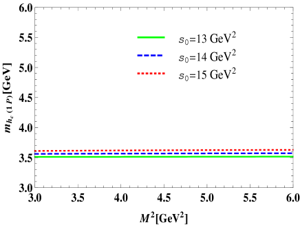
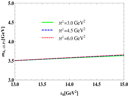
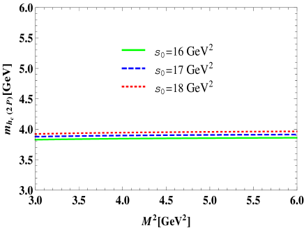
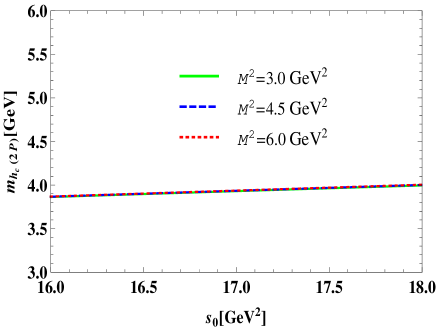
Figure 1: The masses of the mesons $h_{c}(1P,2P)$ in terms of the Borel parameter $M^{2}$ at fixed values of $s_{0}$ (left panel), and in terms of the continuum threshold $s_{0}$ at fixed values of $M^{2}$ (right panel).

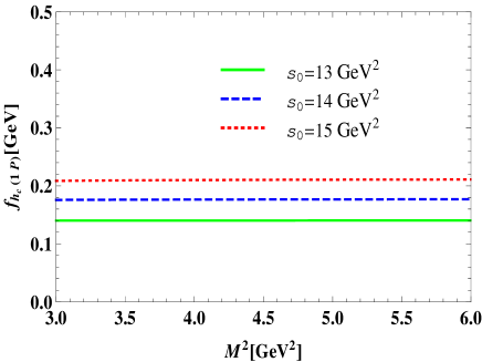
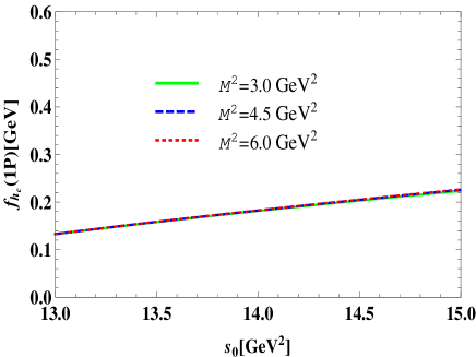
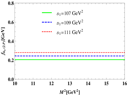
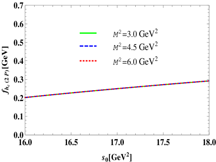
Figure 2: The same as figure 1 but for the decay constants $f_{h_{c}(1P,2P)}$.

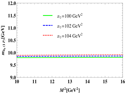
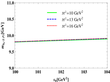
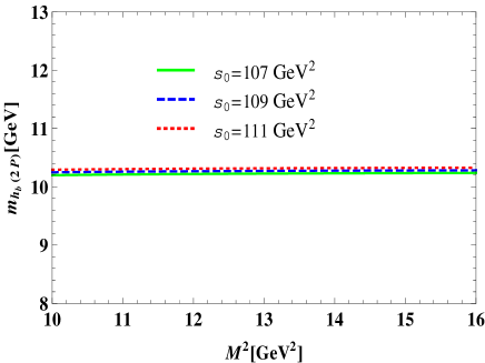
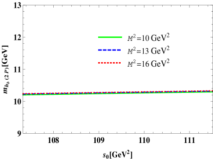
Figure 3: The same as figure 1 but for the masses of the mesons $h_{b}(1P,2P)$.

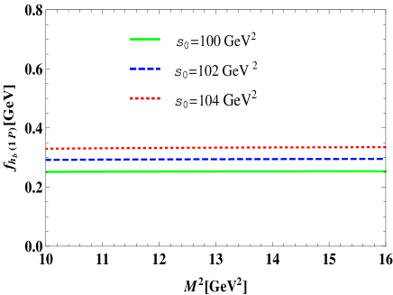
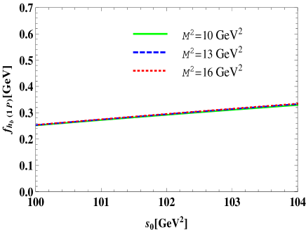
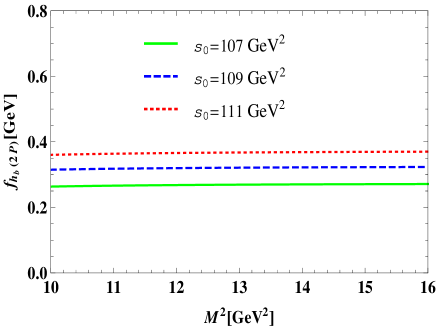
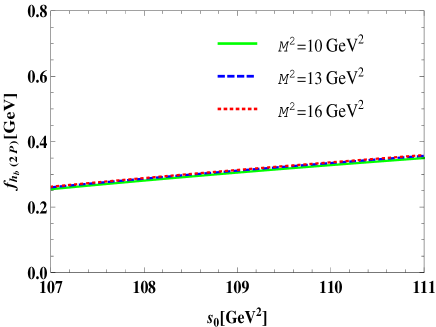
Figure 4: The same as figure 1 but for the decay constants $f_{h_{b}(1P,2P)}$.

IV Concluding Remarks

We have studied the $h_{Q}(1P)$ and $h_{Q}(2P)$ systems employing the QCD sum rule method, where in calculations terms up to dimension eight have been used. We adopted an interpolating current including a derivative and with quantum numbers $J^{PC}=1^{+-}$ for the $h_{Q}(1P)$ and $h_{Q}(2P)$ states. The mass and decay constant of the ground-state mesons $h_{Q}(1P)$ and their first radial excitations $h_{Q}(2P)$ have been extracted from the corresponding sum rules derived in the present study. Our results for the spectroscopic parameters of these mesons, compared with the existing experimental data as well as other theoretical predictions, are presented in Tables 3 and 4.

We should note that recently, in the framework of QCD sum rule method, the mass and decay constant of the $h_{b}$ mesons were calculated in Ref. AgaevZb using a tensor-type interpolating current. For the mass and decay constant of the $h_{b}(1P)$ and $h_{b}(2P)$ mesons in this work the following results were found: for the ground-state $h_{b}(1P)$ meson $m_{h_{b}}(1P)=9886^{+81}_{-78}\ \mathrm{MeV}$ and $f_{h_{b}}=325^{+61}_{-57}\ \mathrm{MeV}$, for its first radial excited state $m_{h_{b}}(2P)=10331^{+108}_{-117}\ \mathrm{MeV}$ and $f_{h_{b}}(2P)=286^{+58}_{-53}\ \mathrm{MeV}$. Obtained in Ref. AgaevZb by using the tensor-type current, the value of the decay constant for $h_{b}(1P)$ is $9.85\%$ higher than, and the value of the decay constant for the $h_{b}(2P)$ state is $10.06\%$ lower than the values extracted in the present work using the axial-vector type current. Any future experimental data on the decay constants will help us to determine which interpolating current is favored for the states under consideration. As for the masses, however, the two studies predict consistent values within the errors. Our predictions on the masses are also in agreements with other theoretical predictions as well as existing experimental data. There are considerable differences among the theoretical predictions on the values of the decay constants. The results of present work may shed light on experimental searches for the $h_{c}(2P)$ state. Besides the predicted masses, the obtained decay constants can be used in theoretical determinations of the total widths of the considered states via analyses of their possible strong, electromagnetic and weak decays. Such theoretical predictions on the widths of these states may help experimental groups to measure the parameters of these states more precisely.

The determination of the basic properties of quarkonia is very important to explain the experimental data exist on the spectrum of the hidden charmed and bottom sectors. Such determinations will enable us to categorize the experimentally observed resonances and precisely determine which of these states belong to the quarkonia resonances and which ones to the class of the quarkonia-like XYZ exotic states that are in agenda of the particle physicists nowadays. We hope that the theoretical studies will improve our knowledge in this regard, and shed light on the experiments in order to obtain more accurate data.

Appendix A The Non-perturbative Part of the Spectral Density

The non-perturbative part of the spectral density used in Eq. (12) is found in terms of the dimension four, six and eight gluon condensates as:

$$\rho^{\mathrm{Nonpert.}}(s) = \Big{\langle}\frac{\alpha_{s}G^{2}}{\pi}\Big{\rangle}\int_{0}^{1}f_{1}(z,s)dz$$ (A.18)

$$+ \Big{\langle}g_{s}^{3}G^{3}\Big{\rangle}\int_{0}^{1}f_{2}(z,s)dz$$

$$+ \Big{\langle}\frac{\alpha_{s}G^{2}}{\pi}\Big{\rangle}^{2}\int_{0}^{1}f_{3}(z,s)dz.$$

In Eq. (A.18) the functions $f_{1}(z,s),\ f_{2}(z,s)$ and $f_{3}(z,s)$ have the explicit forms:

$$f_{1}(z,s) = \frac{1}{24r^{2}}\Big{[}-6r^{2}(s-\Phi)-3r[-2m_{Q}^{2}+sr)]$$

$$\times \delta^{(1)}(s-\Phi)+m_{Q}^{2}s(1+2r)\delta^{(2)}(s-\Phi)\Big{]},$$

$$f_{2}(z,s) = \frac{1}{15\cdot 2^{9}\pi^{2}r^{5}}\Big{\{}\delta^{(4)}(s-\Phi)\Big{(}2m_{Q}^{6}[1+5r(1+r)]$$ (A.20)

$$- m_{Q}^{4}r[7+r(31+23r)]s+6m_{Q}^{2}s^{2}r^{3}(1+2r)$$

$$+ r^{5}s^{3}\Big{)}+2\Big{[}12r^{3}\delta^{(1)}(s-\Phi)[1+5r(1+r)]$$

$$+ 6sr^{3}\delta^{(2)}[1+r(7+11r)]+r\delta^{(3)}\Big{(}-3m_{Q}^{4}[1$$

$$+ 5r(1+r)]+9m_{Q}^{2}sr[1+2r(2+r)]+2s^{2}r^{3}$$

$$\times (2+7r)\Big{)}\Big{]}\Big{\}},$$

and

$$f_{3}(z,s) = \frac{1}{2^{4}\cdot 3^{3}r^{2}}m_{Q}^{2}\pi^{2}\Big{[}6r\delta^{(3)}(s-\Phi)+\delta^{(5)}(s-\Phi)$$

$$\times s(-m_{Q}^{2}+rs)+2\delta^{(4)}(s-\Phi)[-m_{Q}^{2}+s(1+3r)]\Big{]},$$

where we use the following notations

$$\ r=z(z-1),\ \ \Phi=\frac{m_{Q}^{2}}{z(1-z)}.$$ (A.22)

In the above expressions

$$\delta^{(n)}(s-\Phi)=\frac{d^{n}}{ds^{n}}\delta(s-\Phi).$$ (A.23)

References

- (1) P. L. Cho and A. K. Leibovich, Phys. Rev. D 53, 6203 (1996).
- (2) H. Satz, J. Phys. G 32, R25 (2006).
- (3) R. Rapp, D. Blaschke and P. Crochet, Prog. Part. Nucl. Phys. 65, 209 (2010).
- (4) M. B. Voloshin, Prog. Part. Nucl. Phys. 61, 455 (2008).
- (5) J. Beringer et al. [Particle Data Group], Phys. Rev. D 86, 010001 (2012).
- (6) N. Brambilla et al., Eur. Phys. J. C 71, 1534 (2011).
- (7) J. Soto, arXiv:1709.08038 [hep-ph].
- (8) Y. Wang, J. Phys. Conf. Ser. 873, no. 1, 012026 (2017).
- (9) F. De Mori [BESIII Collaboration], Nuovo Cim. C 39, no. 4, 320 (2017).
- (10) D. Ebert, R. N. Faustov and V. O. Galkin, Mod. Phys. Lett. A 20, 875 (2005).
- (11) E. Eichten, K. Gottfried, T. Kinoshita, K. D. Lane and T. M. Yan, Phys. Rev. D 21, 203 (1980).
- (12) M. Cacciari, Nuclear Physics B (Proc. Suppl.) 71, 431-440, (1999).
- (13) B. Fulsom, Proceedings, 2nd Conference on Large Hadron Collider Physics Conference (LHCP 2014): New York, USA, June 2-7 (2014).
- (14) B. Aubert et al. [BaBar Collaboration], Phys. Rev. Lett. 95, 142001 (2005).
- (15) S. K. Choi et al. [Belle Collaboration], Phys. Rev. Lett. 100, 142001 (2008).
- (16) R. Mizuk et al. [Belle Collaboration], Phys. Rev. D 78, 072004 (2008).
- (17) P. Krokovny et al. [Belle Collaboration], Proceedings, 48th Rencontres de Moriond on QCD and High Energy Interactions: La Thuile, Italy, March 9-16,(2013).
- (18) P. C. Vinodkumar, M. Shah and B. Patel, DAE Symp. Nucl. Phys. 57, 656 (2012).
- (19) V. M. Abazov et al. [D0 Collaboration], Phys. Rev. Lett. 117, no. 2, 022003 (2016).
- (20) D. Acosta et al. [CDF Collaboration], Phys. Rev. Lett. 93, 072001 (2004).
- (21) A. Andronic et al., Eur. Phys. J. C 76, no. 3, 107 (2016).
- (22) E. J. Eichten, K. Lane and C. Quigg, Phys. Rev. D 69, 094019 (2004).
- (23) T. Barnes and E. S. Swanson, Phys. Rev. C 77, 055206 (2008).
- (24) J. L. Rosner, Flavor physics and CP violation. Proceedings, 9th International Conference, FPCP 2011, Maale HaChamisha, Israel, May 23-27 (2011).
- (25) C. Baglin et al. [R704 and Annecy(LAPP)-CERN-Genoa-Lyon-Oslo-Rome-Strasbourg-Turin Collaborations], Phys. Lett. B 171, 135 (1986).
- (26) M. Andreotti et al., Phys. Rev. D 72, 032001 (2005).
- (27) J. L. Rosner et al. [CLEO Collaboration], Phys. Rev. Lett. 95, 102003 (2005).
- (28) J. Sonnenschein, Prog. Part. Nucl. Phys. 92, 1 (2017).
- (29) M. Ablikim et al. [BESIII Collaboration], Phys. Rev. Lett. 116, no. 25, 251802 (2016).
- (30) M. Ablikim et al. [BESIII Collaboration], Phys. Rev. Lett. 118, no. 9, 092002 (2017).
- (31) J. P. Lees et al. [BaBar Collaboration], Phys. Rev. D 84, 091101 (2011).
- (32) A. Bondar et al. [Belle Collaboration], Phys. Rev. Lett. 108, 122001 (2012).
- (33) I. Adachi [Belle Collaboration], Flavor physics and CP violation. Proceedings, 9th International Conference, FPCP 2011, Maale HaChamisha,Israel, May 23-27, (2011).
- (34) W. Buchmüller, Current Physics Sources and Comments: Quarkonia, Vol:9, Edited by W. Buchmüller, Elsevier Pub. Com., 2 Dec. (2012).
- (35) A. Ali, J. S. Lange and S. Stone, arXiv:1706.00610 [hep-ph].
- (36) N. Akbar, M. A. Sultan, B. Masud and F. Akram, Phys. Rev. D 95, no. 7, 074018 (2017).
- (37) W. J. Deng, H. Liu, L. C. Gui and X. H. Zhong, Phys. Rev. D 95, no. 3, 034026 (2017).
- (38) Z. Y. Zhou and Z. Xiao, arXiv:1704.04438 [hep-ph].
- (39) Z. Y. Zhou and Z. Xiao, Phys. Rev. D 96, no. 5, 054031 (2017) Erratum: [Phys. Rev. D 96, no. 9, 099905 (2017)].
- (40) M. Bhat, A. P. Monteiro and K. B. Vijaya Kumar, arXiv:1702.06774 [hep-ph].
- (41) P. P. D’Souza, M. Bhat, A. P. Monteiro and K. B. Vijaya Kumar, arXiv:1703.10413 [hep-ph].
- (42) S. Godfrey, AIP Conf. Proc. 132, 262 (1985).
- (43) B. Q. Li and K. T. Chao, Phys. Rev. D 79, 094004 (2009).
- (44) D. Becirevic, G. Duplancic, B. Klajn, B. Melic and F. Sanfilippo, Nucl. Phys. B 883, 306 (2014).
- (45) M. A. Shifman, A. I. Vainshtein and V. I. Zakharov, Nucl. Phys. B 147, 385 (1979).
- (46) M. A. Shifman, A. I. Vainshtein and V. I. Zakharov, Nucl. Phys. B 147, 448 (1979).
- (47) L. J. Reinders, H. Rubinstein and S. Yazaki, Phys. Rept. 127, 1 (1985).
- (48) B. L. Ioffe, Prog. Part. Nucl. Phys. 56, 232 (2006).
- (49) V. M. Belyaev and B. L. Ioffe, Sov. Phys. JETP 57, 716 (1983) [Zh. Eksp. Teor. Fiz. 84, 1236 (1983)].
- (50) C. Patrignani et al. [Particle Data Group], Chin. Phys. C 40, no. 10, 100001 (2016).
- (51) T. Barnes, S. Godfrey and E. S. Swanson, Phys. Rev. D 72, 054026 (2005).
- (52) J. Ferretti and E. Santopinto, Phys. Rev. D 90, no. 9, 094022 (2014).
- (53) S. Godfrey and K. Moats, Phys. Rev. D 92, no. 5, 054034 (2015).
- (54) D. Ebert, R. N. Faustov and V. O. Galkin, Eur. Phys. J. C 71, 1825 (2011).
- (55) J. Segovia, P. G. Ortega, D. R. Entem and F. Fern ndez, Phys. Rev. D 93, no. 7, 074027 (2016).
- (56) J. F. Liu and G. J. Ding, Eur. Phys. J. C 72, 1981 (2012).
- (57) Y. Lu, M. N. Anwar and B. S. Zou, Phys. Rev. D 94, no. 3, 034021 (2016).
- (58) P. Chen, Phys. Rev. D 64, 034509 (2001).
- (59) V. Bashiry, Phys. Rev. D 84, 076008 (2011).
- (60) M. Okamoto et al. [CP-PACS Collaboration], Phys. Rev. D 65, 094508 (2002).
- (61) S. S. Agaev, K. Azizi and H. Sundu, arXiv:1709.03148 [hep-ph].
- (62) G. L. Wang, Phys. Lett. B 650, 15 (2007)
- (63) V. A. Novikov, L. B. Okun, M. A. Shifman, A. I. Vainshtein, M. B. Voloshin and V. I. Zakharov, Phys. Rept. 41, 1 (1978).
- (64) X. X. Wang, W. Wang and C. D. Lu, Phys. Rev. D 79, 114018 (2009).
- (65) Z. G. Wang, Eur. Phys. J. C 73, no. 8, 2533 (2013).