On the solution of Stokes equation on regions with corners

Abstract

In Stokes flow, the stream function associated with the velocity of the fluid satisfies the biharmonic equation. The detailed behavior of solutions to the biharmonic equation on regions with corners has been historically difficult to characterize. The problem was first examined by Lord Rayleigh in 1920; in 1973, the existence of infinite oscillations in the domain Green’s function was proven in the case of the right angle by S. Osher. In this paper, we observe that, when the biharmonic equation is formulated as a boundary integral equation, the solutions are representable by rapidly convergent series of the form $\sum_{j}(c_{j}t^{\mu_{j}}\sin{(\beta_{j}\log{(t)})}+d_{j}t^{\mu_{j}}\cos{(\beta_{j}\log{(t)})})$, where $t$ is the distance from the corner and the parameters $\mu_{j},\beta_{j}$ are real, and are determined via an explicit formula depending on the angle at the corner. In addition to being analytically perspicuous, these representations lend themselves to the construction of highly accurate and efficient numerical discretizations, significantly reducing the number of degrees of freedom required for the solution of the corresponding integral equations. The results are illustrated by several numerical examples.

Keywords: Integral equations, Stokes flow, Polygonal domains, Biharmonic equation, Corners

1 Introduction

In classical potential theory, solutions to elliptic partial differential equations are represented by potentials on the boundaries of the regions. Over the last four decades, several well-conditioned boundary integral representations have been developed for the biharmonic equation with various boundary conditions. These integral representations have been studied extensively when the boundaries of the regions are approximated by a smooth curve (see, [1, 2, 3, 4, 5, 6, 7, 8], for example). In all of these representations, the kernels of the integral equation are at worst weakly singular and, in same cases, even smooth. The corresponding solutions to the integral equations tend to be as smooth as the boundaries of the domains and the incoming data.

However, when the boundary of the region has corners, the solutions to both the differential equation and the corresponding integral equations are known to develop singularities. The solutions to the differential equation have been studied extensively on regions with corners for both Dirichlet and gradient boundary conditions. In particular, the behavior of solutions to the biharmonic equation on a wedge enclosed by straight boundaries $\theta=0$ and $\theta=\alpha$, and a circular arc $r=r_{0}$, where $(r,\theta)$ are polar coordinates, has received much attention over the years. To the best of our knowledge, this particular problem was first studied by Lord Rayleigh in 1920 [9], and over the decades, was studied by A. Dixon [10], Dean and Montagnon [11], Szegö [12], Moffat [13], Williams [14], and Seif [15], to name a few. In 1973, S. Osher showed that the Green’s function for the biharmonic equation on a right angle wedge has infinitely many oscillations in the vicinity of the corner on all but finitely many rays [16]. The more complicated structure of the Green’s function for the biharmonic equation is explained, in part, by the fact that the biharmonic equation does not have a maximum principle associated with it, while, for example, Laplace’s equation does.

While much has been published about the solutions to the differential equation, the solutions of the corresponding integral equation have been studied much less exhaustively. Recently, a detailed analysis of solutions to integral equations corresponding to the Laplace and Helmholtz equations on regions with corners was carried out by the second author and V. Rokhlin [17, 18, 19]. They observed that the solutions to these integral equations can be expressed as rapidly convergent series of singular powers in the Laplace case and Bessel functions of non-integer order in the Helmholtz case.

In this paper, we investigate the solutions to a standard integral equation corresponding to the velocity boundary value problem for Stokes equation. For the velocity boundary value problem, the stream function associated with the velocity field satisfies the biharmonic equation with gradient boundary conditions (it turns out that the same integral equation can be used for Dirichlet boundary conditions, see, for example, [8]). We show that, if the boundary data is smooth on each side of the corner, then the solutions of this integral equation can be expressed a rapidly convergent series of elementary functions of the form $t^{\mu_{j}}\cos{(\beta_{j}\log{|t|})}$ and $t^{\mu_{j}}\sin{(\beta_{j}\log{|t|})}$, where the parameters $\mu_{j},\beta_{j}$ can be computed explicitly by a simple formula depending only on the angle at the corner. Furthermore, we prove that, for any $N$, there exists a linear combination of the first $N$ of these basis functions which satisfies the integral equation with error $O(|t|^{N})$, where $t$ is the distance from the corner.

The detailed information about the analytical behavior of the solution in the vicinity of corners, discussed in this paper, allows for the construction of purpose-made discretizations of the integral equation. These discretizations accurately represent the solutions near corners using far fewer degrees of freedom than graded meshes, which are commonly used in such environments, thereby leading to highly efficient numerical solvers for the integral equation. For an alternative treatment of the differential equation see, for example, [20, 21, 22].

The rest of the paper is organized as follows. In Section 2, we discuss the mathematical preliminaries for the governing equation and it’s reformulation as an integral equation. In Section 3, we derive several analytical results using techniques required for the principal results which are derived in Section 4. We illustrate the performance of the numerical scheme which utilizes the explicit knowledge of the structure of the solution to the integral equation in Section 5. In Section 6, we present generalizations and extensions of the apparatus of this paper. The proof of several results in Section 4 are technical and are presented in Sections 8 and 9.

2 Preliminaries

In this paper, vector-valued quantities are denoted by bold, lower-case letters (e.g. ${\boldsymbol{h}}$), while tensor-valued quantities are bold and upper-case (e.g. $\mathbf{T}$). Subscript indices of non-bold characters (e.g. $h_{j}$ or $T_{jkl}$) are used to denote the entries within a vector (${\boldsymbol{h}}$) or tensor (${\mathbf{T}}$). We use the standard Einstein summation convention; in other words, there is an implied sum taken over the repeated indices of any term (e.g. the symbol $a_{j}b_{j}$ is used to represent the sum $\sum_{j}a_{j}b_{j}$). Let ${\mathcal{C}}^{k}$ denote the space of functions which have $k$ continuous derivatives.

Suppose now that $\Omega$ is a simply connected open subset of ${\mathbb{R}}^{2}$. Let $\Gamma$ denote the boundary of $\Omega$ and suppose that $\Gamma$ is a simple closed curve of length $L$ with $n_{c}$ corners. Let ${\boldsymbol{\gamma}}:[0,L]\to{\mathbb{R}}^{2}$ denote an arc length parameterization of $\Gamma$ in the counter-clockwise direction, and suppose that the location of the corners are given by ${\boldsymbol{\gamma}}(s_{j})$, $j=1,2,\ldots n_{c}$ with $0=s_{1}<s_{2}\ldots<s_{n_{c}}<s_{n_{c}+1}=L$. We assume that the corners all have finite angles, i.e., the region $\Omega$ does not have any cusps. Furthermore, suppose that ${\boldsymbol{\gamma}}$ is analytic on the intervals $(s_{j},s_{j+1})$ for each $j=1,2,\ldots n_{c}$. Let ${\boldsymbol{\tau}}({\boldsymbol{x}})$ and ${\boldsymbol{\nu}}({\boldsymbol{x}})$ denote the positively-oriented unit tangent and the outward unit normal respectively, for ${\boldsymbol{x}}\in\Gamma$. Let $h_{\tau}=h_{j}\tau_{j}$ and $h_{\nu}=h_{j}\nu_{j}$ denote the tangential and normal components of the vector ${\boldsymbol{h}}$ respectively, see Figure 1.

Figure 1: A sample domain $\Omega$ with three corners

Remark 1.

In this section, we will be concerned with regions of the form $\Omega$ described above (see Figure 1).

2.1 Velocity boundary value problem

The equations of incompressible Stokes flow with velocity boundary conditions on a domain $\Omega$ with boundary $\Gamma$ are

$$-\Delta{\boldsymbol{u}}+\nabla p =0\quad\mbox{in }\Omega,$$ (1)

$$\nabla\cdot{\boldsymbol{u}} =0\quad\mbox{in }\Omega,$$ (2)

$${\boldsymbol{u}} ={\boldsymbol{h}}\quad\text{on }\Gamma,$$ (3)

where ${\boldsymbol{u}}$ is the velocity of the fluid, $p$ is the fluid pressure and ${\boldsymbol{h}}$ is the prescribed velocity on the boundary. For any ${\boldsymbol{h}}$ which satisfies

$$\int_{\Gamma}{\boldsymbol{h}}\cdot{\boldsymbol{\nu}}\,dS=0\,,$$ (4)

there exists a unique velocity field ${\boldsymbol{u}}$ and a pressure $p$, defined uniquely up to a constant, that satisfy 1, 2 and 3. We summarize the result in the following lemma (see [23] for a proof).

Lemma 2.

Suppose ${\boldsymbol{h}}\in{\mathbb{L}}^{2}(\Gamma)$ and satisfies $\int_{\Gamma}{\boldsymbol{h}}\cdot{\boldsymbol{\nu}}\,dS=0$ , then there exists a unique velocity ${\boldsymbol{u}}$ and a pressure $p$ which is unique up to a constant which satisfy the velocity boundary value problem 1, 2 and 3.

Remark 3.

The Stokes equation with velocity boundary conditions can be reformulated as a biharmonic equation with gradient boundary conditions. First, we represent the velocity ${\boldsymbol{u}}\colon\Omega\to{\mathbb{R}}^{2}$ as ${\boldsymbol{u}}=\nabla^{\perp}w$, where $w\colon\Omega\to{\mathbb{R}}$ is the stream function associated with the velocity field and $\nabla^{\perp}$ is the operator given by

$$\nabla^{\perp}w=\begin{bmatrix}-\frac{\partial w}{\partial x_{2}}\\ \frac{\partial w}{\partial x_{1}}\end{bmatrix}\,.$$ (5)

Next, we observe that ${\boldsymbol{u}}=\nabla^{\perp}w$ automatically satisfies the divergence free condition 2. Finally, taking the dot product of $\nabla^{\perp}$ with 1, we observe that $w$ satisfies the biharmonic equation with gradient boundary conditions given by

$$\Delta^{2}w =0\quad\text{in }\Omega$$ (6)

$$\nabla^{\perp}w ={\boldsymbol{h}}\quad\text{on }\Gamma\,.$$ (7)

2.2 Integral equation formulation

Following the treatment of [24, 5], the fundamental solution to the Stokes equations (the Stokeslet) is given by

$$G_{j,k}\left({\boldsymbol{x}},{\boldsymbol{y}}\right)=\frac{1}{4\pi}\left[-\log\left|{\boldsymbol{x}}-{\boldsymbol{y}}\right|\delta_{ij}+\frac{\left(x_{j}-y_{j}\right)\left(x_{k}-y_{k}\right)}{\left|{\boldsymbol{x}}-{\boldsymbol{y}}\right|^{2}}\right]\,,\quad j,k\in{1,2}\,,$$ (8)

for ${\boldsymbol{x}},{\boldsymbol{y}}\in{\mathbb{R}}^{2}$, and ${\boldsymbol{x}}\neq{\boldsymbol{y}}$, where $\delta_{ij}$ is the Kronecker delta function. The stress tensor $T_{j,k,\ell}\left({\boldsymbol{x}},{\boldsymbol{y}}\right)$ associated with the Green’s function, or the stresslet, is given by

$$T_{j,k,\ell}\left({\boldsymbol{x}},{\boldsymbol{y}}\right)=-\frac{1}{\pi}\frac{\left(x_{j}-y_{j}\right)\left(x_{k}-y_{k}\right)\left(x_{\ell}-y_{\ell}\right)}{\left|{\boldsymbol{x}}-{\boldsymbol{y}}\right|^{4}}\quad j,k,\ell\in 1,2\,,$$ (9)

${\boldsymbol{x}},{\boldsymbol{y}}\in{\mathbb{R}}^{2}$ and ${\boldsymbol{x}}\neq{\boldsymbol{y}}$. The stresslet ${\mathbf{T}}$ is roughly analogous to a dipole in electrostatics. The double layer Stokes potential is the velocity field due to a surface density of stresslets ${\boldsymbol{\mu}}$ and is defined by

$$\left({\mathcal{D}}_{\Gamma}[{\boldsymbol{\mu}}]({\boldsymbol{x}})\right)_{j}=\int_{\Gamma}T_{k,j,\ell}\left({\boldsymbol{y}},{\boldsymbol{x}}\right)\mathbf{\mu}_{k}\left({\boldsymbol{y}}\right)\nu_{\ell}({\boldsymbol{y}})\,dS_{{\boldsymbol{y}}}\,,\quad j,k,\ell\in 1,2\,,$$ (10)

for ${\boldsymbol{x}}\in{\mathbb{R}}^{2}$. Clearly, ${\mathcal{D}}_{\Gamma}[{\boldsymbol{\mu}}]({\boldsymbol{x}})$ satisfies Stokes equation for ${\boldsymbol{x}}\in\Omega$.

The following lemma describes the behavior of the double layer Stokes potential as ${\boldsymbol{x}}\to{\boldsymbol{x}}_{0}$ where ${\boldsymbol{x}}_{0}\in\Gamma$.

Lemma 4.

Suppose that ${\boldsymbol{\mu}}\colon\Gamma\to{\mathbb{R}}^{2}$ and let $\mathcal{D}_{\Gamma}[{\boldsymbol{\mu}}]\left({\boldsymbol{x}}\right)$ denote a double layer Stokes potential (10). Then $\mathcal{D}_{\Gamma}[{\boldsymbol{\mu}}]\left({\boldsymbol{x}}\right)$ satisfies the jump relation:

$$\lim_{\begin{subarray}{c}{\boldsymbol{x}}\to{\boldsymbol{x}}_{0}\\ {\boldsymbol{x}}\in\Omega\end{subarray}}\mathcal{D}_{\Gamma}[{\boldsymbol{\mu}}]({\boldsymbol{x}}) =-\frac{1}{2}{\boldsymbol{\mu}}({\boldsymbol{x}}_{0})+\text{p.v.}\int_{\Gamma}{\mathbf{K}}_{0}({\boldsymbol{x}}_{0},{\boldsymbol{y}}){\boldsymbol{\mu}}({\boldsymbol{y}})dS_{{\boldsymbol{y}}}\,,$$ (11)

where ${\boldsymbol{x}}_{0},{\boldsymbol{y}}\in\Gamma$, and ${\mathbf{K}}_{0}$ is given by

$${\mathbf{K}}_{0}({\boldsymbol{x}},{\boldsymbol{y}})=-\frac{1}{\pi}\frac{\left({\boldsymbol{y}}-{\boldsymbol{x}}\right)\cdot{\boldsymbol{\nu}}({\boldsymbol{y}})}{\left|{\boldsymbol{x}}-{\boldsymbol{y}}\right|^{4}}\begin{bmatrix}(y_{1}-x_{1})^{2}&(y_{1}-x_{1})(y_{2}-x_{2})\\ (y_{1}-x_{1})(y_{2}-x_{2})&(y_{2}-x_{2})^{2}\end{bmatrix}\,$$ (12)

for ${\boldsymbol{x}},{\boldsymbol{y}}\in\Gamma$ and $\text{p.v.}\int$ denotes a principal value integral.

Remark 5.

A different jump relation holds for the double layer Stokes potential, ${\mathcal{D}}_{\Gamma}[{\boldsymbol{\mu}}]({\boldsymbol{x}})$ at the corner points of the boundary $\Gamma$. However, in the integral equation framework, point values of the density at the corner points are irrelevant from the perspective of computing the velocity ${\mathcal{D}}_{\Gamma}[{\boldsymbol{\mu}}]$ in the region $\Omega$. In the remainder of the paper, we ignore the point behavior of the density ${\boldsymbol{\mu}}$ at the corners.

The following lemma states that the kernel ${\mathbf{K}}_{0}$ is smooth if the boundary $\Gamma$ is smooth.

Lemma 6.

The kernel ${\mathbf{K}}_{0}$ is ${\mathcal{C}}^{k-2}$ if ${\boldsymbol{\gamma}}$ is ${\mathcal{C}}^{k}$ with limiting values

$$\lim_{t\to s}{\mathbf{K}}_{0}({\boldsymbol{\gamma}}(t),{\boldsymbol{\gamma}}(s))=-\frac{1}{\pi}\kappa({\boldsymbol{\gamma}}(t))\begin{bmatrix}\gamma_{1}^{\prime}(t)^{2}&\gamma_{1}^{\prime}(t)\gamma_{2}^{\prime}(t)\\ \gamma_{1}^{\prime}(t)\gamma_{2}^{\prime}(t)&\gamma_{2}^{\prime}(t)^{2}\\ \end{bmatrix}\,,$$ (13)

where $\kappa({\boldsymbol{\gamma}}(t))$ is the curvature at ${\boldsymbol{\gamma}}(t)$. Furthermore, ${\mathbf{K}}_{0}$ is analytic if ${\boldsymbol{\gamma}}$ is analytic.

The following theorem reduces the velocity boundary value problem 1, 2 and 3 to an integral equation on the boundary by representing ${\boldsymbol{u}}$ as double layer Stokes potential with unknown density ${\boldsymbol{\mu}}$, i.e.

$${\boldsymbol{u}}({\boldsymbol{x}})={\mathcal{D}}_{\Gamma}[{\boldsymbol{\mu}}]({\boldsymbol{x}})\,\quad{\boldsymbol{x}}\in\Omega.$$ (14)

Lemma 7.

Suppose ${\boldsymbol{h}}\in{\mathbb{L}}^{2}(\Gamma)$ and that $\int_{\Gamma}{\boldsymbol{h}}\cdot{\boldsymbol{\nu}}\,dS=0$. Then there exists a unique solution ${\boldsymbol{\mu}}\in{\mathbb{L}}^{2}(\Gamma)$ which satisfies

$$-\frac{1}{2}{\boldsymbol{\mu}}({\boldsymbol{x}})+\text{p.v.}\int_{\Gamma}{\mathbf{K}}_{0}({\boldsymbol{x}},{\boldsymbol{y}}){\boldsymbol{\mu}}({\boldsymbol{y}})\,dS_{{\boldsymbol{y}}}={\boldsymbol{h}}({\boldsymbol{x}})\,,\quad{\boldsymbol{x}}\in\Gamma\,,$$ (15)

and $\int_{\Gamma}{\boldsymbol{\mu}}\cdot{\boldsymbol{\nu}}\,dS=0$. Furthermore, ${\boldsymbol{u}}({\boldsymbol{x}})={\mathcal{D}}_{\Gamma}[{\boldsymbol{\mu}}]({\boldsymbol{x}})$ satisfies Stokes equations 1 and 2, along with the boundary conditions ${\boldsymbol{u}}({\boldsymbol{x}})={\boldsymbol{h}}({\boldsymbol{x}})$ for ${\boldsymbol{x}}\in\Gamma$.

Proof. See, for example, [5] for a proof. $\blacksquare$

The following lemma extends Lemma 7 to the case where the boundary $\Gamma$ is an open arc.

Lemma 8.

Suppose ${\boldsymbol{h}}\in{\mathbb{L}}^{2}(\Gamma)$ then there exists a unique solution ${\boldsymbol{\mu}}\in{\mathbb{L}}^{2}(\Gamma)$ which satisfies

$$-\frac{1}{2}{\boldsymbol{\mu}}({\boldsymbol{x}})+\text{p.v.}\int_{\Gamma}{\mathbf{K}}_{0}({\boldsymbol{x}},{\boldsymbol{y}}){\boldsymbol{\mu}}({\boldsymbol{y}})\,dS_{{\boldsymbol{y}}}={\boldsymbol{h}}({\boldsymbol{x}})\quad{\boldsymbol{x}}\in\Gamma\,,$$ (16)

where ${\mathbf{K}}_{0}$ is defined by 12.

2.3 Integral equation in tangential and normal coordinates

It turns out that it is convenient to represent both the velocity on the boundary ${\boldsymbol{h}}$ and the solution of the integral equation ${\boldsymbol{\mu}}$ in terms of their tangential and normal coordinates, denoted by ${\boldsymbol{h}}=(h_{\tau},h_{\nu})$ and ${\boldsymbol{\mu}}=(\mu_{\tau},\mu_{\nu})$ respectively, as opposed to their Cartesian coordinates. In this section, we discuss the representation in the tangential and normal coordinates of the double layer Stokes potential, and the corresponding integral equation for the velocity boundary value problem.

Let $\mathbf{R}({\boldsymbol{x}})$ denote the unitary transformation that converts vectors expressed in Cartesian coordinates to vectors expressed in tangential and normal components, i.e.

$$\mathbf{R}({\boldsymbol{x}})=\begin{bmatrix}\tau_{1}({\boldsymbol{x}})&\tau_{2}({\boldsymbol{x}})\\ \nu_{1}({\boldsymbol{x}})&\nu_{2}({\boldsymbol{x}})\end{bmatrix}\,\quad{\boldsymbol{x}}\in\Gamma.$$ (17)

Let $\mathbf{R}^{*}({\boldsymbol{x}})$ denote the adjoint of $\mathbf{R}({\boldsymbol{x}})$. Suppose ${\boldsymbol{u}}({\boldsymbol{x}})=(u_{1}({\boldsymbol{x}}),u_{2}({\boldsymbol{x}}))$ is the double layer Stokes potential with density ${\boldsymbol{\mu}}({\boldsymbol{x}})=(\mu_{\tau}({\boldsymbol{x}}),\mu_{\nu}({\boldsymbol{x}}))$, given by

$${\boldsymbol{u}}({\boldsymbol{x}})=\tilde{{\mathcal{D}}}_{\Gamma}[{\boldsymbol{\mu}}]({\boldsymbol{x}})\,\quad{\boldsymbol{x}}\in\Omega,$$ (18)

where

$$\left(\tilde{{\mathcal{D}}}_{\Gamma}[{\boldsymbol{\mu}}]({\boldsymbol{x}})\right)_{j}=\int_{\Gamma}T_{k,j,\ell}({\boldsymbol{y}},{\boldsymbol{x}})\left(\mathbf{R}^{*}({\boldsymbol{y}})\cdot\begin{bmatrix}\mu_{\tau}({\boldsymbol{y}})\\ \mu_{\nu}({\boldsymbol{y}})\end{bmatrix}\right)_{k}\nu_{\ell}({\boldsymbol{y}})dS_{{\boldsymbol{y}}}\,,\quad j,k,\ell=1,2\,,$$ (19)

where ${\boldsymbol{x}}\in\Omega$. The following theorem reduces the velocity boundary value problem 1, 2 and 3 to an integral equation on the boundary in the rotated frame.

Lemma 9.

Suppose ${\boldsymbol{h}}=(h_{\tau},h_{\nu})\in{\mathbb{L}}^{2}(\Gamma)$ and that $\int_{\Gamma}h_{\nu}\,dS=0$. Then there exists a unique solution ${\boldsymbol{\mu}}=(\mu_{\tau},\mu_{\nu})\in{\mathbb{L}}^{2}(\Gamma)$ which satisfies

$$-\frac{1}{2}\begin{bmatrix}\mu_{\tau}({\boldsymbol{x}})\\ \mu_{\nu}({\boldsymbol{x}})\end{bmatrix}+\text{p.v.}\int_{\Gamma}{\mathbf{K}}({\boldsymbol{x}},{\boldsymbol{y}})\begin{bmatrix}\mu_{\tau}({\boldsymbol{y}})\\ \mu_{\nu}({\boldsymbol{y}})\end{bmatrix}\,dS_{{\boldsymbol{y}}}=\begin{bmatrix}h_{\tau}({\boldsymbol{x}})\\ h_{\nu}({\boldsymbol{x}})\end{bmatrix}\,,\quad{\boldsymbol{x}}\in\Gamma\,,$$ (20)

along with $\int_{\Gamma}\mu_{\nu}\,dS=0$, where

$${\mathbf{K}}({\boldsymbol{x}},{\boldsymbol{y}})=\mathbf{R}({\boldsymbol{x}}){\mathbf{K}}_{0}({\boldsymbol{x}},{\boldsymbol{y}})\mathbf{R}^{*}({\boldsymbol{y}})\,,\quad{\boldsymbol{x}},{\boldsymbol{y}}\in\Gamma.$$ (21)

Furthermore, ${\boldsymbol{u}}({\boldsymbol{x}})=\tilde{{\mathcal{D}}}_{\Gamma}[{\boldsymbol{\mu}}]({\boldsymbol{x}})$ satisfies Stokes equations 1 and 2, along with the boundary conditions ${\boldsymbol{u}}({\boldsymbol{x}})={\boldsymbol{h}}({\boldsymbol{x}})$ for ${\boldsymbol{x}}\in\Gamma$.

Proof. The result is a straightforward consequence of Lemma 7. $\blacksquare$

The following lemma extends Lemma 9 to the case where the boundary $\Gamma$ is an open arc.

Lemma 10.

Suppose that $\Gamma$ is an open arc and suppose ${\boldsymbol{h}}=(h_{\tau},h_{\nu})\in{\mathbb{L}}^{2}(\Gamma)$, then there exists a unique solution ${\boldsymbol{\mu}}=(\mu_{\tau},\mu_{\nu})\in{\mathbb{L}}^{2}(\Gamma)$ which satisfies

$$-\frac{1}{2}\begin{bmatrix}\mu_{\tau}({\boldsymbol{x}})\\ \mu_{\nu}({\boldsymbol{x}})\end{bmatrix}+\text{p.v.}\int_{\Gamma}{\mathbf{K}}({\boldsymbol{x}},{\boldsymbol{y}})\begin{bmatrix}\mu_{\tau}({\boldsymbol{y}})\\ \mu_{\nu}({\boldsymbol{y}})\end{bmatrix}\,dS_{{\boldsymbol{y}}}=\begin{bmatrix}h_{\tau}({\boldsymbol{x}})\\ h_{\nu}({\boldsymbol{x}})\end{bmatrix}\,,\quad{\boldsymbol{x}}\in\Gamma\,,$$ (22)

where ${\mathbf{K}}$ is defined by 21.

2.4 Integral equations on the wedge

In order to investigate the behavior of solutions to integral equation 20 on polygonal domains, we first analyze the local behavior of solutions on a wedge (see Figure 2). The following observation reduces the analysis of the solution $\mu$ on polygonal domains to its local behavior on a single wedge.

Observation 11.

Let $\Omega$ be a polygonal domain, and let ${\boldsymbol{\mu}}$ be the solution to the integral equation 20 corresponding to a prescribed velocity ${\boldsymbol{h}}$ on the boundary. Using Lemma 9, we know that there exists a unique density ${\boldsymbol{\mu}}$ in ${\mathbb{L}}^{2}(\Gamma)$. Let $\Gamma_{1}$ denote a wedge in the vicinity of one of the corners. Then, the integral equation 20 can be rewritten as

$$-\frac{1}{2}\begin{bmatrix}\mu_{\tau}({\boldsymbol{x}})\\ \mu_{\nu}({\boldsymbol{x}})\end{bmatrix}+\text{p.v.}\int_{\Gamma_{1}}{\mathbf{K}}({\boldsymbol{x}},{\boldsymbol{y}})\begin{bmatrix}\mu_{\tau}({\boldsymbol{y}})\\ \mu_{\nu}({\boldsymbol{y}})\end{bmatrix}dS_{{\boldsymbol{y}}}={\boldsymbol{h}}({\boldsymbol{x}})-\int_{\Gamma\setminus\Gamma_{1}}{\mathbf{K}}({\boldsymbol{x}},{\boldsymbol{y}})\begin{bmatrix}\mu_{\tau}({\boldsymbol{y}})\\ \mu_{\nu}({\boldsymbol{y}})\end{bmatrix}dS_{{\boldsymbol{y}}}\,$$ (23)

for ${\boldsymbol{x}}\in\Gamma_{1}$. For any ${\boldsymbol{\mu}}\in{\mathbb{L}}^{2}(\Gamma)$, the integral

$$\int_{\Gamma\setminus\Gamma_{1}}{\mathbf{K}}({\boldsymbol{x}},{\boldsymbol{y}})\begin{bmatrix}\mu_{\tau}({\boldsymbol{y}})\\ \mu_{\nu}({\boldsymbol{y}})\end{bmatrix}dS_{{\boldsymbol{y}}}\,,$$ (24)

is a smooth function for ${\boldsymbol{x}}\in\Gamma_{1}$. Using Lemma 10, the unique solution to the integral equation 23 is the restriction of the solution ${\boldsymbol{\mu}}({\boldsymbol{x}})$ to integral equation 20 from $\Gamma$ to $\Gamma_{1}$. Moreover, in nearly all practical settings, the prescribed velocity ${\boldsymbol{h}}$ is also a piecewise smooth function on either side of the corner. Thus, to understand the local behavior of the solution ${\boldsymbol{\mu}}$ to the integral equation on polygonal domains, it suffices to analyze the restriction of the integral equation to an open wedge with piecewise smooth velocity prescribed on either side.

Suppose ${\boldsymbol{\gamma}}(t):[-1,1]\to{\mathbb{R}}^{2}$ is a wedge with interior angle $\pi\theta$ and side length $1$ on either side of the corner, parametrized by arc-length (see, Figure 2).

Figure 2: A wedge with interior angle $\pi\theta$

In a slight misuse of notation, let $\mu_{\tau}(t)$ denote $\mu_{\tau}({\boldsymbol{\gamma}}(t))$ for all $-1<t<1$. Likewise, let $\mu_{\nu}(t),h_{\tau}(t)$, and $h_{\nu}(t)$ denote $\mu_{\nu}({\boldsymbol{\gamma}}(t))$, $h_{\tau}({\boldsymbol{\gamma}}(t))$ and $h_{\nu}({\boldsymbol{\gamma}}(t))$, respectively. The integral equation 22 for the velocity boundary value problem is then given by

$$-\frac{1}{2}\begin{bmatrix}\mu_{\tau}(t)\\ \mu_{\nu}(t)\end{bmatrix}+\text{p.v.}\int_{-1}^{1}{\mathbf{K}}({\boldsymbol{\gamma}}(t),{\boldsymbol{\gamma}}(s))\begin{bmatrix}\mu_{\tau}(s)\\ \mu_{\nu}(s)\end{bmatrix}\,ds=\begin{bmatrix}h_{\tau}(t)\\ h_{\nu}(t)\end{bmatrix}\,,\,\,-1<t<1\,,$$ (25)

where ${\mathbf{K}}$ is defined by 21. In this case, the kernel ${\mathbf{K}}$ has a simple form which is given by the following lemma.

Lemma 12.

Suppose ${\boldsymbol{\gamma}}:[-1,1]\to{\mathbb{R}}^{2}$ is defined by the formula

$${\boldsymbol{\gamma}}(t)=\begin{cases}-t\cdot(\cos(\pi\theta),\sin(\pi\theta))&\mbox{if $-1<t<0$}\,,\\ (t,0)&\mbox{if $0<t<1$}\,.\end{cases}$$ (26)

Suppose further that $k_{j}(s,t)$, $j=1,2,3,4$, are defined by

$$k_{1}(s,t) =\frac{t\sin(\pi\theta)}{\pi\left(s^{2}+t^{2}+2st\cos(\pi\theta)\right)^{2}}(s+t\cos{(\pi\theta)})(s\cos{(\pi\theta)}+t)\,,$$ (27)

$$k_{2}(s,t) =\frac{t\sin(\pi\theta)}{\pi\left(s^{2}+t^{2}+2st\cos(\pi\theta)\right)^{2}}t\sin{(\pi\theta)}(t+s\cos{(\pi\theta)})\,,$$ (28)

$$k_{3}(s,t) =-\frac{t\sin(\pi\theta)}{\pi\left(s^{2}+t^{2}+2st\cos(\pi\theta)\right)^{2}}(s+t\cos{(\pi\theta)})s\sin{(\pi\theta)}\,,$$ (29)

$$k_{4}(s,t) =-\frac{t\sin(\pi\theta)}{\pi\left(s^{2}+t^{2}+2st\cos(\pi\theta)\right)^{2}}st\sin^{2}{(\pi\theta)}\,.$$ (30)

for all $-1<s,t<1$. If $0<t<1$, then

$${\mathbf{K}}({\boldsymbol{\gamma}}(t),{\boldsymbol{\gamma}}(s))=\begin{cases}\displaystyle\begin{bmatrix}k_{1}(s,t)&k_{2}(s,t)\\ k_{3}(s,t)&k_{4}(s,t)\end{bmatrix}&\mbox{if $-1<s<0$}\,,\vspace*{3pt}\\ \begin{bmatrix}0&0\\ 0&0\end{bmatrix}&\mbox{if $0<s<1$}\,.\end{cases}$$ (31)

Likewise, if $-1<t<0$, then

$${\mathbf{K}}({\boldsymbol{\gamma}}(t),{\boldsymbol{\gamma}}(s))=\begin{cases}\begin{bmatrix}0&0\\ 0&0\end{bmatrix}&\mbox{if $-1<s<0$}\,,\vspace*{3pt}\\ \displaystyle\begin{bmatrix}-k_{1}(s,t)&k_{2}(s,t)\\ k_{3}(s,t)&-k_{4}(s,t)\end{bmatrix}&\mbox{if $0<s<1$}\,.\end{cases}$$ (32)

Remark 13.

The zero blocks in 31 and 32 are due to the fact that the self-interaction of the kernel on the sides is zero (in fact, the kernel vanishes on any straight line).

In the following theorem, we show that, when $\Gamma$ is a wedge, the integral equation 25 decouples into two independent integral equations on the interval $[0,1]$.

Theorem 14.

Suppose $\mu_{\tau},\mu_{\nu}$ are functions in ${\mathbb{L}}^{2}[-1,1]$. Let $h_{\tau},h_{\nu}$ be defined by 25. We denote the odd and the even parts of a function $f$ by $f_{o}$ and $f_{e}$ respectively, where

$$f_{o}(s)=\frac{1}{2}\left(f(s)-f(-s)\right)\,,\quad\text{and}\,,\quad f_{e}(s)=\frac{1}{2}\left(f(s)+f(-s)\right)\,,$$ (33)

for $-1<s<1$. Then for $0<t<1$,

$$\begin{bmatrix}h_{\tau,e}(t)\\ h_{\nu,o}(t)\end{bmatrix}=-\frac{1}{2}\begin{bmatrix}\mu_{\tau,e}(t)\\ \mu_{\nu,o}(t)\end{bmatrix}-\int_{0}^{1}\begin{bmatrix}k_{1,1}(s,t)&k_{1,2}(s,t)\\ k_{2,1}(s,t)&k_{2,2}(s,t)\end{bmatrix}\begin{bmatrix}\mu_{\tau,e}(s)\\ \mu_{\nu,o}(s)\end{bmatrix}\,ds\,,$$ (34)

and

$$\begin{bmatrix}h_{\tau,o}(t)\\ h_{\nu,e}(t)\end{bmatrix}=-\frac{1}{2}\begin{bmatrix}\mu_{\tau,o}(t)\\ \mu_{\nu,e}(t)\end{bmatrix}+\int_{0}^{1}\begin{bmatrix}k_{1,1}(s,t)&k_{1,2}(s,t)\\ k_{2,1}(s,t)&k_{2,2}(s,t)\end{bmatrix}\begin{bmatrix}\mu_{\tau,o}(s)\\ \mu_{\nu,e}(s)\end{bmatrix}\,ds\,,$$ (35)

where $k_{j,\ell}(s,t)$, $j,\ell=1,2$, are given by

$$k_{1,1}(s,t) =\frac{1}{2}\left(k_{1}(s,-t)-k_{1}(-s,t)\right)=\frac{t\sin{(\pi\theta)}(s-t\cos{(\pi\theta)})(t-s\cos{(\pi\theta)})}{\pi(s^{2}+t^{2}-2st\cos{(\pi\theta)})^{2}}\,,$$ (36)

$$k_{1,2}(s,t) =\frac{1}{2}\left(-k_{2}(s,-t)+k_{2}(-s,t)\right)=\frac{t^{2}\sin^{2}{(\pi\theta)}(t-s\cos{(\pi\theta)})}{\pi(s^{2}+t^{2}-2st\cos{(\pi\theta)})^{2}}\,,$$ (37)

$$k_{2,1}(s,t) =\frac{1}{2}\left(k_{3}(s,-t)-k_{3}(-s,t)\right)=\frac{st\sin^{2}{(\pi\theta)}(s-t\cos{(\pi\theta)})}{\pi(s^{2}+t^{2}-2st\cos{(\pi\theta)})^{2}}\,,$$ (38)

$$k_{2,2}(s,t) =\frac{1}{2}\left(-k_{4}(s,-t)+k_{4}(-s,t)\right)=\frac{st^{2}\sin^{3}{(\pi\theta)}}{\pi(s^{2}+t^{2}-2st\cos{(\pi\theta)})^{2}}\,,$$ (39)

for all $0<s,t<1$.

Proof. Substituting the expression for the kernel ${\mathbf{K}}$ given by 31 and 32 in 25, we get

$$\begin{bmatrix}h_{\tau}(t)\\ h_{\nu}(t)\end{bmatrix}=-\frac{1}{2}\begin{bmatrix}\mu_{\tau}(t)\\ \mu_{\nu}(t)\end{bmatrix}+\int_{-1}^{0}\begin{bmatrix}k_{1}(s,t)&k_{2}(s,t)\\ k_{3}(s,t)&k_{4}(s,t)\end{bmatrix}\begin{bmatrix}\mu_{\tau}(s)\\ \mu_{\nu}(s)\end{bmatrix}\,ds\,,$$ (40)

for $0<t<1$ and

$$\begin{bmatrix}h_{\tau}(t)\\ h_{\nu}(t)\end{bmatrix}=-\frac{1}{2}\begin{bmatrix}\mu_{\tau}(t)\\ \mu_{\nu}(t)\end{bmatrix}+\int_{0}^{1}\begin{bmatrix}-k_{1}(s,t)&k_{2}(s,t)\\ k_{3}(s,t)&-k_{4}(s,t)\end{bmatrix}\begin{bmatrix}\mu_{\tau}(s)\\ \mu_{\nu}(s)\end{bmatrix}\,ds\,,$$ (41)

for $-1<t<0$. Then, making the change of variable $s\to-s$ in 40 and the change of variable $t\to-t$ in 41, we get

$$\begin{bmatrix}h_{\tau}(t)\\ h_{\nu}(t)\end{bmatrix}=-\frac{1}{2}\begin{bmatrix}\mu_{\tau}(t)\\ \mu_{\nu}(t)\end{bmatrix}+\int_{0}^{1}\begin{bmatrix}k_{1}(-s,t)&k_{2}(-s,t)\\ k_{3}(-s,t)&k_{4}(-s,t)\end{bmatrix}\begin{bmatrix}\mu_{\tau}(-s)\\ \mu_{\nu}(-s)\end{bmatrix}\,ds\,,$$ (42)

for $0<t<1$ and

$$\begin{bmatrix}h_{\tau}(-t)\\ h_{\nu}(-t)\end{bmatrix}=-\frac{1}{2}\begin{bmatrix}\mu_{\tau}(-t)\\ \mu_{\nu}(-t)\end{bmatrix}+\int_{0}^{1}\begin{bmatrix}-k_{1}(s,-t)&k_{2}(s,-t)\\ k_{3}(s,-t)&-k_{4}(s,-t)\end{bmatrix}\begin{bmatrix}\mu_{\tau}(s)\\ \mu_{\nu}(s)\end{bmatrix}\,ds\,,$$ (43)

for $0<t<1$. Finally, combining 42 and 43, we get

$$\begin{bmatrix}h_{\tau,e}(t)\\ h_{\nu,o}(t)\end{bmatrix} =-\frac{1}{2}\begin{bmatrix}\mu_{\tau,e}(t)\\ \mu_{\nu,o}(t)\end{bmatrix}-\int_{0}^{1}\begin{bmatrix}k_{1,1}(s,t)&k_{1,2}(s,t)\\ k_{2,1}(s,t)&k_{2,2}(s,t)\end{bmatrix}\begin{bmatrix}\mu_{\tau,e}(s)\\ \mu_{\nu,o}(s)\end{bmatrix}\,ds\,,$$ (44)

$$\begin{bmatrix}h_{\tau,o}(t)\\ h_{\nu,e}(t)\end{bmatrix} =-\frac{1}{2}\begin{bmatrix}\mu_{\tau,o}(t)\\ \mu_{\nu,e}(t)\end{bmatrix}+\int_{0}^{1}\begin{bmatrix}k_{1,1}(s,t)&k_{1,2}(s,t)\\ k_{2,1}(s,t)&k_{2,2}(s,t)\end{bmatrix}\begin{bmatrix}\mu_{\tau,o}(s)\\ \mu_{\nu,e}(s)\end{bmatrix}\,ds\,.$$ (45)

$\blacksquare$

We represent the given velocity ${\boldsymbol{h}}$ on the boundary in terms of its tangential $h_{\tau}$ and normal $h_{\nu}$ components. We decompose both $h_{\tau}$ and $h_{\nu}$ into their odd and even parts, denoted by $h_{\tau,o}$, $h_{\tau,e}$, and $h_{\nu,o}$, $h_{\nu,e}$ as follows:

$$h_{\tau,o}(t)=\frac{1}{2}\left(h_{\tau}(t)-h_{\tau}(-t)\right)\,,\quad h_{\tau,e}(t)=\frac{1}{2}\left(h_{\tau}(t)+h_{\tau}(-t)\right)\,,$$ (46)

$$h_{\nu,o}(t)=\frac{1}{2}\left(h_{\nu}(t)-h_{\nu}(-t)\right)\,,\quad h_{\nu,e}(t)=\frac{1}{2}\left(h_{\nu}(t)+h_{\nu}(-t)\right)\,,$$ (47)

$-1<t<1$. Suppose now that the densities $\mu_{\tau,e}$, $\mu_{\tau,o}$, $\mu_{\nu,e}$, and $\mu_{\nu,o}$ denote the solutions the integral equations 44 and 45 with $h_{\tau,e}$, $h_{\tau,o}$, $h_{\nu,e}$, and $h_{\nu,o}$ defined in 46 and 47. Then ${\boldsymbol{\mu}}(t)=(\mu_{\tau}(t),\mu_{\nu}(t))$ defined by

$$\begin{bmatrix}\mu_{\tau}(t)\\ \mu_{\nu}(t)\end{bmatrix}=\frac{1}{2}\begin{bmatrix}\mu_{\tau,o}(t)+\mu_{\tau,e}(t)\\ \mu_{\nu,o}(t)+\mu_{\nu,e}(t)\end{bmatrix}\,,\quad-1<t<1\,,$$ (48)

satisfies integral equation 25.

Thus, the integral equation 25 clearly splits into two cases:

• Tangential odd, normal even: the tangential components of both the velocity field ${\boldsymbol{h}}$ and the density ${\boldsymbol{\mu}}$, $h_{\tau}(t)$ and $\mu_{\tau}(t)$, are odd functions of $t$ and the normal components $h_{\nu}(t)$ and $\mu_{\nu}(t)$ are even functions of $t$.

• Tangential even, normal odd: the tangential components of both the velocity field ${\boldsymbol{h}}$ and the density ${\boldsymbol{\mu}}$, $h_{\tau}(t)$ and $\mu_{\tau}(t)$, are even functions of $t$ and the normal components $h_{\nu}(t)$ and $\mu_{\nu}(t)$ are odd functions of $t$.

3 Analytical Apparatus

In this section, we investigate integrals of the form

$$\int_{0}^{1}k_{j,\ell}(s,t)s^{z}\,ds\,,\quad j,\ell=1,2\,,$$ (49)

for $0<t<1$, where $z\in{\mathbb{C}}$ with $\text{Re}(z)>-1$, and $k_{j,\ell}$ are defined in 36, 37, 38 and 39. We use the branch of $\log$ with $\mathrm{arg}(s)\in[0,2\pi)$ for the definition of $s^{z}$. The principal result of this section is Theorem 22.

On inspecting the kernels $k_{j,\ell}(s,t)$, $j,\ell=1,2$, we observe that it suffices to evaluate integrals of the form

$$I(z,\theta,t)=\frac{1}{\pi}\int_{0}^{1}\frac{s^{z}}{(s^{2}+t^{2}-2st\cos{(\pi\theta)})^{2}}\,ds\,,\quad\text{for }0<t<1\,,$$ (50)

where $\text{Re}(z)>-1$. Using standard techniques in complex analysis, we first derive an expression for the above integral from $0$ to $\infty$ in the following lemma.

Remark 15.

Clearly, the integral 50, is well-defined for $\text{Re}(z)>-1$; in Lemmas 17 and 18, we make the additional assumption that $\text{Re}(z)<3$. This restriction will be eliminated later.

Remark 16.

We consider integrals of the form 50 for $\theta$ in the complex plane, since we will eventually complexify $\theta$ to better understand the behavior of integral equations 44 and 45 on $\theta\in(0,2)$.

Lemma 17.

Suppose $z\in{\mathbb{C}}$, $-1<\text{Re}(z)<3$, $z\neq 0,1,2$, and $\theta\in{\mathbb{C}}$. Then

$$I_{1}(z,\theta,t)=\frac{1}{\pi}\int_{0}^{\infty}\frac{s^{z}}{\left(s^{2}+t^{2}-2st\cos{(\pi\theta)}\right)^{2}}\,ds=a(z,\theta)t^{z-3}\,,$$ (51)

for $0<t<1$ where

$$a(z,\theta)=\frac{z\sin{(2\pi\theta)}\cos{(\pi(1-\theta)z)}+2\sin{(\pi(1-\theta)z)}\left(1-z\sin^{2}{(\pi\theta)}\right)}{4\sin{(\pi z)}\sin^{3}{(\pi\theta)}}\,.$$ (52)

Proof. Let $\Gamma_{\text{key}}=\Gamma_{\varepsilon}\cup\Gamma_{1}\cup\Gamma_{R}\cup\Gamma_{2}$ denote a keyhole contour where

$$\Gamma_{\varepsilon}=\left\{-\varepsilon e^{ix}\,,\quad-\frac{\pi}{2}<x<\frac{\pi}{2}\right\}\,, \quad\Gamma_{1}=\left\{x+i\varepsilon\,,\quad 0\leq x\leq\sqrt{R^{2}-\varepsilon^{2}}\right\}\,,$$

$$\Gamma_{R}=\left\{Re^{ix}\,,\quad x_{0}<x<2\pi-x_{0}\right\}\,, \quad\Gamma_{2}=\left\{x-i\varepsilon\,,\quad 0\leq x\leq\sqrt{R^{2}-\varepsilon^{2}}\right\}\,,$$

where $x_{0}=\arctan{\varepsilon/R}$, see Figure 3.

Figure 3: A keyhole contour

Using Cauchy’s integral theorem,

$$\int_{\Gamma_{\text{key}}} \frac{s^{z}}{\left(s^{2}+t^{2}-2st\cos{(\pi\theta)}\right)^{2}}\,ds=\left(\int_{\Gamma_{\varepsilon}}+\int_{\Gamma_{1}}+\int_{\Gamma_{R}}+\int_{\Gamma_{2}}\right)\frac{s^{z}}{\left(s-te^{i\pi\theta}\right)^{2}\left(s-te^{i\pi(2-\theta)}\right)^{2}}\,ds\,,$$ (53)

$$=2\pi i\left(\frac{d}{ds}\left(\frac{s^{z}}{\left(s-te^{i\pi(2-\theta)}\right)^{2}}\right)\Bigg{|}_{s=te^{i\pi\theta}}+\frac{d}{ds}\left(\frac{s^{z}}{\left(s-te^{i\pi\theta}\right)^{2}}\right)\Bigg{|}_{s=te^{i\pi(2-\theta)}}\right)\,,$$ (54)

$$=-\frac{2\pi t^{z-3}}{\sin^{3}{(\pi\theta)}}\left((z-2)\left(e^{i\pi\theta z}-e^{2\pi iz}e^{-i\pi\theta z}\right)-z\left(e^{i\pi\theta(z-2)}-e^{2\pi iz}e^{-i\pi\theta(z-2)}\right)\right)\,,$$ (55)

for $0<t<1$. Suppose $0<t<1$, then there exists a constant $M_{1}<\infty$ such that

$$\left|\frac{s^{z}}{\left(s^{2}+t^{2}-2st\cos{(\pi\theta)}\right)^{2}}\right|\leq M_{1}\varepsilon^{\text{Re}(z)}\,,$$ (56)

for all $s\in\Gamma_{\varepsilon}$. Taking the limit as $\varepsilon\to 0$, we get

$$\lim_{\varepsilon\to 0}\left|\int_{\Gamma_{\varepsilon}}\frac{s^{z}}{\left(s^{2}+t^{2}-2st\cos{(\pi\theta)}\right)^{2}}\,ds\right|\leq\lim_{\varepsilon\to 0}\pi M_{1}\varepsilon^{\text{Re}(z)+1}=0\,\,,$$ (57)

since $\text{Re}(z)>-1$. Similarly, for $0<t<1$, there exists a constant $M_{2}<\infty$ such that

$$\left|\frac{s^{z}}{\left(s^{2}+t^{2}-2st\cos{(\pi\theta)}\right)^{2}}\right|\leq\frac{M_{2}}{R^{4-\text{Re}(z)}}\,,$$ (58)

for all $s\in\Gamma_{R}$. Taking the limit as $R\to\infty$, we get

$$\lim_{R\to\infty}\left|\int_{\Gamma_{R}}\frac{s^{z}}{\left(s^{2}+t^{2}-2st\cos{(\pi\theta)}\right)^{2}}\,ds\right|\leq\lim_{R\to\infty}\frac{2\pi M}{R^{3-\text{Re}(z)}}=0\,\,,$$ (59)

since $\text{Re}(z)<3$. On $\Gamma_{1}$ and $\Gamma_{2}$, taking the limits as $\varepsilon\to 0$ and $R\to\infty$, we get

$$\lim_{\varepsilon\to 0}\lim_{R\to\infty}\int_{\Gamma_{1}}\frac{s^{z}}{\left(s^{2}+t^{2}-2st\cos{(\pi\theta)}\right)^{2}}\,ds =I_{1}(z,\theta,t)\,,$$ (60)

$$\lim_{\varepsilon\to 0}\lim_{R\to\infty}\int_{\Gamma_{2}}\frac{s^{z}}{\left(s^{2}+t^{2}-2st\cos{(\pi\theta)}\right)^{2}}\,ds =-e^{2\pi iz}I_{1}(z,\theta,t)\,.$$ (61)

The result follows by taking the limit $\varepsilon\to 0$ and $R\to\infty$ in 55, and using 57, 59, 60 and 61. $\blacksquare$

Suppose now that $I_{2}(z,\theta,t)$ is defined by

$$I_{2}(z,\theta)=\int_{1}^{\infty}\frac{s^{z}}{(s^{2}+t^{2}-2st\cos{(\pi\theta)})^{2}}\,ds\,,$$ (62)

for $0<t<1$. Clearly,

$$I(z,\theta,t)=I_{1}(z,\theta,t)-I_{2}(z,\theta,t)\,,$$ (63)

where $I(z,\theta,t)$ is given by 50 and $I_{1}(z,\theta,t)$ by 51. In the following lemma, we compute an expression for $I_{2}(z,\theta,t)$ by deriving a Taylor expansion for

$$f(s,t,\theta)=\frac{1}{(s^{2}+t^{2}-2st\cos{(\pi\theta)})^{2}}\,,\quad\text{for }|s|>1,|t|<1\,.$$

Lemma 18.

Suppose that $\theta\in{\mathbb{C}}$. Then for all $|t|<1$ and $|s|>1$

$$f(s,t,\theta)=\frac{1}{\left(s^{2}+t^{2}-2st\cos{(\pi\theta)}\right)^{2}}=\sum_{n=0}^{\infty}a_{n}(s,\theta)t^{n}\,,$$ (64)

where

$$a_{n}(s,\theta)=\frac{1}{4s^{n+4}\sin^{3}{(\pi\theta)}}\left((n+3)\sin{((n+1)\pi\theta)}-(n+1)\sin{((n+3)\pi\theta)}\right)\,.$$ (65)

Furthermore, for $-1<\text{Re}(z)<3$, and $z\neq 0,1,2$,

$$I_{2}(z,\theta,t)=\frac{1}{\pi}\int_{1}^{\infty}s^{z}f(s,t,\theta)\,ds=\sum_{n=0}^{\infty}F(n,z,\theta)t^{n}\,,$$ (66)

where

$$F(n,z,\theta)=\frac{(n+1)\sin{((n+3)\pi\theta)}-(n+3)\sin((n+1)\pi\theta)}{4\pi(-z+n+3)\sin^{3}{(\pi\theta)}}\,.$$ (67)

Proof. For fixed $|s|>1$, $f(s,t)$ is analytic in $|t|<1$. Using Cauchy’s integral formula, the coefficients of the Taylor series are given by

$$a_{n}(s,\theta) =\frac{1}{2\pi i}\int_{|\xi|=1}\frac{f(s,\xi,\theta)}{\xi^{n+1}}d\xi=\frac{1}{2\pi}\int_{0}^{2\pi}e^{-inx}f(s,e^{ix},\theta)\,dx\,,$$ (68)

$$=\frac{1}{2\pi}\int_{0}^{2\pi}\frac{e^{-inx}}{(s-e^{i(\pi\theta+x)})^{2}(s-e^{i(-\pi\theta+x)})^{2}}\,dx\,,$$ (69)

$$=\frac{1}{2\pi s^{4}}\int_{0}^{2\pi}\frac{e^{-inx}}{\left(1-\frac{e^{i(\pi\theta+x)}}{s}\right)^{2}\left(1-\frac{e^{i(-\pi\theta+x)}}{s}\right)^{2}}\,dx\,.$$ (70)

Using the Taylor expansion of $1/(1-x)^{2}$ given by

$$\frac{1}{(1-x)^{2}}=\sum_{n=0}^{\infty}(n+1)x^{n}\,,$$ (71)

for $0<x<1$, equation 70 simplifies to,

$$a_{n}(s,\theta)=\frac{1}{2\pi}\frac{1}{s^{4}}\int_{0}^{2\pi}e^{-inx}\sum_{\ell=0}^{\infty}\sum_{m=0}^{\infty}(\ell+1)(m+1)\frac{e^{i(\ell+m)x+(\ell-m)\pi\theta}}{s^{\ell+m}}\,dx$$ (72)

Due to the orthogonality of the Fourier basis $\{e^{inx}\}$ in ${\mathbb{L}}^{2}[0,2\pi]$, the only terms that contribute to the integral in 72 are when $\ell+m=n$. Thus,

$$a_{n}(s,\theta)=\frac{1}{s^{n+4}}\sum_{\ell+m=n}(\ell+1)(m+1)e^{i(\ell-m)\pi\theta}=\frac{e^{-in\pi\theta}}{s^{n+4}}\sum_{\ell=0}^{n}(\ell+1)(n-\ell+1)e^{2i\ell\pi\theta}\,.$$ (73)

The result for the Taylor series for $f(s,t)$ then follows by using

$$\sum_{\ell=0}^{n}\ell^{p}e^{i\ell x}=\frac{d^{p}}{dx^{p}}\left(\frac{1-e^{i(n+1)x}}{1-e^{ix}}\right)\,\quad p=0,1,2\,.$$ (74)

Given the Taylor expansion for $f(s,t)$, the integral $I_{2}(z,\theta,t)$ can be computed by switching the order of summation and integration and using

$$\int_{1}^{\infty}s^{z}a_{n}(s,\theta)\,ds=F(n,z,\theta)\,,$$ (75)

which concludes the proof. $\blacksquare$

Remark 19.

If $m$ is an integer, the functions $a_{n}(s,\theta)$ and $F(n,z,\theta)$ defined in 65 and 67 respectively, remain bounded as $\theta\to m$:

$$\lim_{\theta\to m}a_{n}(s,\theta)=-\frac{(n+1)(n+2)(n+3)}{6s^{n+4}}\,, \quad\lim_{\theta\to m}F(n,z,\theta)=-\frac{(n+1)(n+2)(n+3)}{6\pi(-z+n+3)}\,,$$

when $m$ is even, and

$$\lim_{\theta\to m}a_{n}(s,\theta)=(-1)^{n}\frac{(n+1)(n+2)(n+3)}{6s^{n+4}}\,, \quad\lim_{\theta\to m}F(n,z,\theta)=(-1)^{n}\frac{(n+1)(n+2)(n+3)}{6\pi(-z+n+3)}\,,$$

when $m$ is odd.

Using Lemmas 17 and 18, we compute $I(z,\theta,t)$ in the following theorem.

Theorem 20.

Suppose $-1<\text{Re}(z)<3$, and $z\neq 0,1,2$, then

$$I(z,\theta,t)=\int_{0}^{1}\frac{s^{z}}{(s^{2}+t^{2}-2st\cos{(\pi\theta)})^{2}}=a(z,\theta)t^{z-3}-\sum_{n=1}^{\infty}F(n,z,\theta)t^{n}\,,$$ (76)

for $0<t<1$.

We observe that both the expressions on the left and right of 76 are analytic functions of $z$ for $\text{Re}(z)>-1$ and $z$ not an integer. In the following theorem, we extend the definition of $I(z,\theta,t)$ to $\text{Re}(z)>-1$ and $z$ not an integer.

Theorem 21.

Suppose that $z\in{\mathbb{C}}$, $\text{Re}(z)>-1$, $z\neq 0,1,2\ldots$, and $\theta\in{\mathbb{C}}$. Then

$$I(z,\theta,t)=\int_{0}^{1}\frac{s^{z}}{(s^{2}+t^{2}-2st\cos{(\pi\theta)})^{2}}=a(z,\theta)t^{z-3}-\sum_{n=1}^{\infty}F(n,z,\theta)t^{n}\,,$$ (77)

for $0<t<1$.

Proof. The result follows from 76 and using analytic continuation. $\blacksquare$

We now present the principal result of this section in the following theorem.

Theorem 22.

Suppose $z\in{\mathbb{C}}$, $\text{Re}(z)>-1$, $z\neq 0,1,2,\ldots$, and $\theta\in{\mathbb{C}}$. Recall that,

$$k_{1,1}(s,t) =\frac{t\sin{(\pi\theta)}(s-t\cos{(\pi\theta)})(t-s\cos{(\pi\theta)})}{\pi(s^{2}+t^{2}-2st\cos{(\pi\theta)})^{2}}\,,$$ (78)

$$k_{1,2}(s,t) =\frac{t^{2}\sin^{2}{(\pi\theta)}(t-s\cos{(\pi\theta)})}{\pi(s^{2}+t^{2}-2st\cos{(\pi\theta)})^{2}}\,,$$ (79)

$$k_{2,1}(s,t) =\frac{st\sin^{2}{(\pi\theta)}(s-t\cos{(\pi\theta)})}{\pi(s^{2}+t^{2}-2st\cos{(\pi\theta)})^{2}}\,,$$ (80)

$$k_{2,2}(s,t) =\frac{st^{2}\sin^{3}{(\pi\theta)}}{\pi(s^{2}+t^{2}-2st\cos{(\pi\theta)})^{2}}\,,$$ (81)

for $0<s,t<1$. Then

$$\int_{0}^{1}k_{1,1}(s,t)s^{z}ds =a_{1,1}(z,\theta)\cdot t^{z}+\sum_{n=1}^{\infty}F_{1,1}(n,z,\theta)\cdot t^{n}\,,$$ (82)

$$\int_{0}^{1}k_{1,2}(s,t)s^{z}ds =a_{1,2}(z,\theta)\cdot t^{z}+\sum_{n=2}^{\infty}F_{1,2}(n,z,\theta)\cdot t^{n}\,,$$ (83)

$$\int_{0}^{1}k_{2,1}(s,t)s^{z}ds =a_{2,1}(z,\theta)\cdot t^{z}+\sum_{n=1}^{\infty}F_{2,1}(n,z,\theta)\cdot t^{n}\,,$$ (84)

$$\int_{0}^{1}k_{2,2}(s,t)s^{z}ds =a_{2,2}(z,\theta)\cdot t^{z}+\sum_{n=2}^{\infty}F_{2,2}(n,z,\theta)\cdot t^{n}\,,$$ (85)

for $0<t<1$, where

$$a_{1,1}(z,\theta) =\frac{1}{2\sin{(\pi z)}}\left[(z+1)\sin{(\pi\theta)}\cos{(\pi z(1-\theta))}-\sin{(\pi(z(1-\theta)+\theta))}\right]\,,$$ (86)

$$a_{1,2}(z,\theta) =-\frac{1}{2\sin{(\pi z)}}(z-1)\sin{(\pi\theta)}\sin{(\pi z(1-\theta))}\,,$$ (87)

$$a_{2,1}(z,\theta) =\frac{1}{2\sin{(\pi z)}}(z+1)\sin{(\pi\theta)}\sin{(\pi z(1-\theta))}\,,$$ (88)

$$a_{2,2}(z,\theta) =\frac{1}{2\sin{(\pi z)}}\left[(z+1)\sin{(\pi\theta)}\cos{(\pi z(1-\theta))}+\sin{(\pi(z(1-\theta)-\theta))}\right]\,,$$ (89)

and

$$F_{1,1}(n,z,\theta) =\frac{n\sin{(\pi\theta)}\cos{(n\pi\theta)}+\cos{(\pi\theta)}\sin{(n\pi\theta)}}{2\pi(n-z)}\,,$$ (90)

$$F_{1,2}(n,z,\theta) =\frac{(n-1)\sin{(\pi\theta)}\sin{(n\pi\theta)}}{2\pi(n-z)}\,,$$ (91)

$$F_{2,1}(n,z,\theta) =-\frac{(n+1)\sin{(\pi\theta)}\sin{(n\pi\theta)}}{2\pi(n-z)}\,,$$ (92)

$$F_{2,2}(n,z,\theta) =\frac{n\sin{(\pi\theta)}\cos{(n\pi\theta)}-\cos{(\pi\theta)}\sin{(n\pi\theta)}}{2\pi(n-z)}\,.$$ (93)

Proof. The result follows from observing that

$$\int_{0}^{1}k_{1,1}(s,t)s^{z}\,ds =-\frac{\sin{(2\pi\theta)}}{2}\left(t\cdot I(z+2,\theta,t)+t^{3}\cdot I(z,\theta,t)\right)$$ (94)

$$\hskip 21.52771pt+t^{2}(1+\cos^{2}{(\pi\theta)})\cdot I(z+1,\theta,t)\,,$$

$$\int_{0}^{1}k_{1,2}(s,t)s^{z}\,ds =t^{2}\sin^{2}{(\pi\theta)}\left(t\cdot I(z,\theta,t)-\cos{(\pi\theta)}I(z+1,\theta,t)\right)\,,$$ (95)

$$\int_{0}^{1}k_{2,1}(s,t)s^{z}\,ds =t\sin^{2}{(\pi\theta)}\left(I(z+2,\theta,t)-t\cos{(\pi\theta)}\cdot I(z+1,\theta,t)\right)\,,$$ (96)

$$\int_{0}^{1}k_{2,2}(s,t)s^{z}\,ds =t^{2}\sin^{3}{(\pi\theta)}\cdot I(z+1,\theta,t)\,,$$ (97)

and using the formula for $I(z,\theta,t)$ derived in Theorem 21. $\blacksquare$

4 Analysis of the integral equation

Suppose that ${\boldsymbol{\gamma}}(t):[-1,1]\to{\mathbb{R}}^{2}$ is a wedge with interior angle $\pi\theta$ and side length $1$ on either side of the corner, parametrized by arc length (see Figure 2). Suppose further that the odd and the even parts of a function $f$ are denoted by $f_{o}$ and $f_{e}$ respectively (see 33). In Section 2.4, we observed that the integral equation

$$-\frac{1}{2}\begin{bmatrix}\mu_{\tau}(t)\\ \mu_{\nu}(t)\end{bmatrix}+\text{p.v.}\int_{-1}^{1}{\mathbf{K}}({\boldsymbol{\gamma}}(t),{\boldsymbol{\gamma}}(s))\begin{bmatrix}\mu_{\tau}(s)\\ \mu_{\nu}(s)\end{bmatrix}\,ds=\begin{bmatrix}h_{\tau}(t)\\ h_{\nu}(t)\end{bmatrix}\,,\,\,-1<t<1\,,$$ (98)

simplifies into two uncoupled integral equations on the interval [0,1], given by

$$-\frac{1}{2}\begin{bmatrix}\mu_{\tau,o}(t)\\ \mu_{\nu,e}(t)\end{bmatrix}+\int_{0}^{1}\begin{bmatrix}k_{1,1}(s,t)&k_{1,2}(s,t)\\ k_{2,1}(s,t)&k_{2,2}(s,t)\end{bmatrix}\begin{bmatrix}\mu_{\tau,o}(s)\\ \mu_{\nu,e}(s)\end{bmatrix}\,ds\,=\begin{bmatrix}h_{\tau,o}(t)\\ h_{\nu,e}(t)\end{bmatrix}\,,$$ (99)

for $0<t<1$, and

$$-\frac{1}{2}\begin{bmatrix}\mu_{\tau,e}(t)\\ \mu_{\nu,o}(t)\end{bmatrix}-\int_{0}^{1}\begin{bmatrix}k_{1,1}(s,t)&k_{1,2}(s,t)\\ k_{2,1}(s,t)&k_{2,2}(s,t)\end{bmatrix}\begin{bmatrix}\mu_{\tau,e}(s)\\ \mu_{\nu,o}(s)\end{bmatrix}\,ds\,=\begin{bmatrix}h_{\tau,e}(t)\\ h_{\nu,o}(t)\end{bmatrix}\,,$$ (100)

for $0<t<1$, where ${\mathbf{K}}$ is defined in 21 and the kernels $k_{j,\ell}(s,t)$, $j,\ell=1,2$, are defined in 36, 37, 38 and 39. As in Section 2.4, we refer to 99 as the tangential odd, normal even case and to 100 as the tangential even, normal odd case.

In Section 4.1, we investigate equation 99, i.e., the tangential odd, normal even case. We determine two countable collections of values $p_{n,j},q_{n,j},z_{n,j}\in{\mathbb{C}}$, $n=1,2,\ldots$, $j=1,2$, depending on the angle $\pi\theta$, such that if $\mu_{\tau,o}(t)$, and $\mu_{\nu,e}(t)$ are defined by

$$\mu_{\tau,o}(t)=p_{n,j}\cdot|t|^{z_{n,j}}\mathop{\mathrm{sgn}}(t)\,,\quad\text{and}\quad\mu_{\nu,e}(t)=q_{n,j}\cdot|t|^{z_{n,j}}\,,$$ (101)

then the corresponding components of the velocity $h_{\tau,o}(t)$ and $h_{\nu,e}(t)$, defined by 99 are smooth. We also prove the converse. Suppose that $N$ is a positive integer. Suppose further that $\alpha_{n},\beta_{n}\in{\mathbb{C}}$, $n=0,1,2\ldots N$, and $h_{\tau,o}(t)$ and $h_{\nu,e}(t)$ are given by

$$h_{\tau,o}(t)=\left(\sum_{n=0}^{N}\alpha_{n}|t|^{n}\right)\mathop{\mathrm{sgn}}(t)\,,\quad\text{and}\quad h_{\nu,e}(t)=\sum_{n=0}^{N}\beta_{n}|t|^{n}\,,$$ (102)

for $-1<t<1$. Then for all but countably many $0<\theta<2$, there exist unique numbers $c_{n},d_{n}\in{\mathbb{C}}$, $n=0,1,\ldots N$, such that $\mu_{\tau,o}(t)$ and $\mu_{\nu,e}(t)$ defined by

$$\mu_{\tau,o}(t) =\left(c_{0}+\sum_{n=1}^{N}c_{n}p_{n,1}|t|^{z_{n,1}}+d_{n}p_{n,2}|t|^{z_{n,2}}\right)\mathop{\mathrm{sgn}}(t)\,,$$ (103)

$$\mu_{\nu,e}(t) =d_{0}+\sum_{n=1}^{N}c_{n}q_{n,1}|t|^{z_{n,1}}+d_{n}q_{n,2}|t|^{z_{n,2}}\,,$$ (104)

for $-1<t<1$ satisfy equation 99 with error $O(|t|^{N+1})$. We prove this result in Theorem 36.

Similarly, in Section 4.2, we investigate equation 100, i.e., the tangential even, normal odd case. We determine two countable collections of values $p_{n,j},q_{n,j},z_{n,j}\in{\mathbb{C}}$, $n=1,2,\ldots$, $j=1,2$, depending on the angle $\pi\theta$, such that, if $\mu_{\tau,e}(t)$, and $\mu_{\nu,o}(t)$ are defined by

$$\mu_{\tau,e}(t)=p_{n,j}\cdot|t|^{z_{n,j}}\,,\quad\text{and}\quad\mu_{\nu,o}(t)=q_{n,j}\cdot|t|^{z_{n,j}}\mathop{\mathrm{sgn}}{(t)}\,,$$ (105)

then the corresponding components of the velocity $h_{\tau,e}(t)$ and $h_{\nu,o}(t)$, defined by 100 are smooth. We also prove the converse. Suppose that $N$ is a positive integer. Suppose further that $\alpha_{n},\beta_{n}\in{\mathbb{C}}$, $n=0,1,2\ldots N$, and $h_{\tau,e}(t)$ and $h_{\nu,o}(t)$ are given by

$$h_{\tau,e}(t)=\sum_{n=0}^{N}\alpha_{n}|t|^{n}\,,\quad\text{and}\quad h_{\nu,o}(t)=\left(\sum_{n=0}^{N}\beta_{n}|t|^{n}\right)\mathop{\mathrm{sgn}}(t)\,,$$ (106)

for $-1<t<1$. Then for all but countably many $0<\theta<2$, there exist unique numbers $c_{n},d_{n}\in{\mathbb{C}}$, $n=0,1,\ldots N$, such that $\mu_{\tau,e}(t)$ and $\mu_{\nu,o}(t)$ defined by

$$\mu_{\tau,e}(t) =c_{0}+\sum_{n=1}^{N}c_{n}p_{n,1}|t|^{z_{n,1}}+d_{n}p_{n,2}|t|^{z_{n,2}}\,,$$ (107)

$$\mu_{\nu,o}(t) =\left(d_{0}+\sum_{n=1}^{N}c_{n}q_{n,1}|t|^{z_{n,1}}+d_{n}q_{n,2}|t|^{z_{n,2}}\right)\mathop{\mathrm{sgn}}{(t)}\,,$$ (108)

for $-1<t<1$ satisfy equation 100 with error $O(|t|^{N+1})$. We prove this result in Theorem 43.

Remark 23.

Although we use the same symbols for the countable collection of values $p_{n,j}$, $q_{n,j}$, and $z_{n,j}$, $n=1,2\ldots$, $j=1,2$, for the tangential even, normal odd case are and the tangential odd, normal even case, their values are in fact different—they are defined by different formulae.

Remark 24.

We note that the the real and imaginary parts of the function $|t|^{z}$ are given by $|t|^{\alpha}\cos{(\beta\log{|t|})}$ and $|t|^{\alpha}\sin{(\beta\log|t|)}$ respectively, where $z=\alpha+$i$\beta$. Analogous results where the density ${\boldsymbol{\mu}}$ is expressed in terms of the functions $|t|^{\alpha}\cos{(\beta\log|t|)}$ and $|t|^{\alpha}\sin{(\beta\log|t|)}$, as opposed to $|t|^{z}$, can be derived for both the tangential odd, normal even case, and the tangential even, normal odd case.

4.1 Tangential odd, normal even case

In this section, we investigate the tangential odd, normal even case (see equation 99). In Section 4.1.1, we determine the values $p_{n,j}$, $q_{n,j}$ and $z_{n,j}$, $n=1,2,\ldots$, $j=1,2$, in 101 for which the resulting components of the velocity are smooth functions. In Section 4.1.2, we show that, for every ${\boldsymbol{h}}$ of the form 102, there exists a density ${\boldsymbol{\mu}}$ of the form 103 and 104, which satisfies the integral equation 99 to order $N$.

4.1.1 The values of $p_{n,j}$, $q_{n,j}$, and $z_{n,j}$ in 101

Suppose that $\mu_{\tau,o}(t)$ and $\mu_{\nu,e}(t)$ are given by

$$\mu_{\tau,o}(t)=p\cdot|t|^{z}\mathop{\mathrm{sgn}}(t)\,,\quad\text{and}\quad\mu_{\nu,e}(t)=q\cdot|t|^{z}\,,$$ (109)

for $-1<t<1$, where $p,q,z\in{\mathbb{C}}$. In this section, we determine the values of $p,q$ and $z$ such that $h_{\tau,o}(t)$ and $h_{\nu,e}(t)$ defined by

$$\begin{bmatrix}h_{\tau,o}(t)\\ h_{\nu,e}(t)\end{bmatrix}=-\frac{1}{2}\begin{bmatrix}\mu_{\tau,o}(t)\\ \mu_{\nu,e}(t)\end{bmatrix}+\int_{0}^{1}\begin{bmatrix}k_{1,1}(s,t)&k_{1,2}(s,t)\\ k_{2,1}(s,t)&k_{2,2}(s,t)\end{bmatrix}\begin{bmatrix}\mu_{\tau,o}(s)\\ \mu_{\nu,e}(s)\end{bmatrix}\,ds\,,$$ (110)

are smooth functions of $t$ for $0<t<1$, where the kernels $k_{j,\ell}(s,t)$, $j,\ell=1,2$, are defined in 36, 37, 38 and 39. The principal result of this section is Theorem 32.

The following lemma describes sufficient conditions for $p,q$, and $z$ such that, if ${\boldsymbol{\mu}}$ is defined by 109, then the velocity ${\boldsymbol{h}}$ given by 110 is smooth.

Theorem 25.

Suppose that $\theta\in(0,2)$, $z$ is not an integer, and $z$ satisfies $\det{{\mathbf{A}}(z,\theta)}=0$, where

$${\mathbf{A}}(z,\theta)=-\frac{1}{2}{\mathbf{I}}+\begin{bmatrix}a_{1,1}(z,\theta)&a_{1,2}(z,\theta)\\ a_{2,1}(z,\theta)&a_{2,2}(z,\theta)\end{bmatrix}\,,$$ (111)

${\mathbf{I}}$ is the $2\times 2$ identity matrix, and $a_{j,\ell}(z,\theta)$, $j,\ell=1,2$, are given by 86, 87, 88 and 89. Furthermore, suppose that $(p,q)\in{\mathcal{N}}\{{\mathbf{A}}(z,\theta)\}$, where ${\mathcal{N}}\{{\mathbf{A}}\}$ denotes the null space of the matrix ${\mathbf{A}}$. Suppose finally that

$$\mu_{\tau,o}(t)=p\cdot t^{z}\,,\quad\text{and}\quad\mu_{\nu,e}(t)=q\cdot t^{z}\,,$$ (112)

for $0<t<1$. Then $h_{\tau,o}(t)$ and $h_{\nu,e}(t)$ defined by 110 satisfy

$$\begin{bmatrix}h_{\tau,o}(t)\\ h_{\nu,e}(t)\end{bmatrix}=\sum_{n=1}^{\infty}{\mathbf{F}}(n,z,\theta)\begin{bmatrix}p\\ q\end{bmatrix}\cdot t^{n}\,,$$ (113)

for $0<t<1$, where

$${\mathbf{F}}(n,z,\theta)=\begin{bmatrix}F_{1,1}(n,z,\theta)&F_{1,2}(n,z,\theta)\\ F_{2,1}(n,z,\theta)&F_{2,2}(n,z,\theta)\end{bmatrix}\,,$$ (114)

and $F_{j,\ell}(n,z,\theta)$, $j,\ell=1,2$, are given by 90, 91, 92 and 93.

Proof. Substituting $\mu_{\tau,o}(t)=p\cdot t^{z}$ and $\mu_{\nu,e}(t)=q\cdot t^{z}$ in 110 and using Theorem 22, we get

$$\begin{bmatrix}h_{\tau,o}(t)\\ h_{\nu,e}(t)\end{bmatrix} =\begin{bmatrix}-1/2p\cdot t^{z}+\int_{0}^{1}\left(p\cdot k_{1,1}(s,t)+q\cdot k_{1,2}(s,t)\right)s^{z}\,ds\\ -1/2q\cdot t^{z}+\int_{0}^{1}\left(p\cdot k_{2,1}(s,t)+q\cdot k_{2,2}(s,t)\right)s^{z}\,ds\\ \end{bmatrix}\,,$$ (115)

$$={\mathbf{A}}(z,\theta)\begin{bmatrix}p\\ q\end{bmatrix}t^{z}+\sum_{n=1}^{\infty}{\mathbf{F}}(n,z,\theta)\begin{bmatrix}p\\ q\end{bmatrix}\cdot t^{n}\,,$$ (116)

Since $(p,q)\in{\mathcal{N}}\{{\mathbf{A}}(z,\theta)\}$, we note that ${\mathbf{A}}(z,\theta)\cdot(p,q)=(0,0)$ and thus

$$\begin{bmatrix}h_{\tau,o}(t)\\ h_{\nu,e}(t)\end{bmatrix}=\sum_{n=1}^{\infty}\begin{bmatrix}F_{1,1}(n,z,\theta)&F_{1,2}(n,z,\theta)\\ F_{2,1}(n,z,\theta)&F_{2,2}(n,z,\theta)\end{bmatrix}\begin{bmatrix}p\\ q\end{bmatrix}\cdot t^{n}\,.$$ (117)

$\blacksquare$

A straightforward calculation shows that

$$\det{{\mathbf{A}}(z,\theta)}=\frac{\left(z\sin{(\pi\theta)}-\sin{(\pi z\theta)}\right)\left(z\sin{(\pi\theta)}-\sin{(\pi z(2-\theta))}\right)}{4\sin^{2}{(\pi z)}}$$ (118)

Thus, if $z$ is not an integer and either

$$z\sin{(\pi\theta)}-\sin{(\pi z(2-\theta))}=0\,,$$ (119)

or

$$z\sin{(\pi\theta)}-\sin{(\pi z\theta)}=0\,,$$ (120)

then $\det{{\mathbf{A}}(z,\theta)}=0$.

Remark 26.

If $z$ satisfies the implicit relations 119 and 120, we have that $\det{{\mathbf{A}}(z,\theta)=0}$. It is then straightforward to determine $p$ and $q$ via an explicit formula in terms of the entries of ${\mathbf{A}}(z,\theta)$, since $(p,q)\in{\mathcal{N}}({\mathbf{A}}(z,\theta))$.

In the following theorem, we prove the existence of the implicit functions $z(\theta)$ defined by 119 and 120 on the interval $\theta\in(0,2)$.

Theorem 27.

Suppose that $N\geq 2$ is an integer. Then there exists $3N-2$ real numbers $\theta_{1},\theta_{2},\ldots\theta_{3N-2}\in(0,2)$ such that the following holds. Suppose that $D$ is the strip in the upper half plane with $0<\text{Re}(\theta)<2$ that includes the interval $(0,2)\setminus\{\theta_{j}\}_{j=1}^{3N-2}$, i.e.

$$D=\{\theta\in{\mathbb{C}}\,:\,\text{Re}(\theta)\in(0,2)\,,\quad 0\leq\text{Im}(\theta)<\infty\}\setminus\{\theta_{j}\}_{j=1}^{3N-2}\,.$$ (121)

Then, there exists a simply connected open set $D\subset V\subset{\mathbb{C}}$ and analytic functions $z_{n,1}(\theta):V\to{\mathbb{C}}$, $n=1,2\ldots N$, which satisfy

$$z\sin{(\pi\theta)}-\sin{(\pi z(2-\theta))}=0\,,\quad z(1)=n\,,$$ (122)

for $\theta\in V$, and analytic functions $z_{n,2}(\theta):V\to{\mathbb{C}}$, $n=2,3,\ldots N$, which satisfy

$$z\sin{(\pi\theta)}-\sin{(\pi z\theta)}=0\,,\quad z(1)=n\,,$$ (123)

for $\theta\in V$ (see Figure 4 for an illustrative domain $V$). Moreover, the functions $z_{n,1}(\theta)$, $n=1,2\ldots N$, do not take integer values for all $\theta\in V\setminus\{1\}$, and satisfy $\det{{\mathbf{A}}(z_{n,1}(\theta),\theta)}=0$, $n=1,2\ldots N$, for all $\theta\in V$ (see 111 and 118). Similarly, the functions $z_{n,2}(\theta)$, $n=2,3,\ldots N$, do not take integer values for all $\theta\in V\setminus\{1\}$, and satisfy $\det{{\mathbf{A}}(z_{n,2}(\theta),\theta)}=0$, $n=2,3\ldots N$, for all $\theta\in V$ (see 111 and 118).

Proof. The proof is technical and is contained in Section 8. $\blacksquare$

Figure 4: An illustrative domain $V$ for the case $N=2$, where $\theta_{1},\theta_{2},\ldots\theta_{5}$ are the combined branch points of the functions $z_{1,1}(\theta)$, $z_{2,1}(\theta)$, and $z_{2,2}(\theta)$. The large dashes are used to denote the interval $(0,2)$ for reference. The thin dashes are the locations of the branch cuts at $\theta_{1},\theta_{2}\ldots\theta_{5}$.

Remark 28.

In fact, the real numbers $\theta_{1},\theta_{2}\ldots\theta_{3N-2}$ are the combined branch points of the functions $z_{n,1}(\theta)$, $n=1,2,\ldots N$, and $z_{n,2}(\theta)$, $n=2,3,\ldots N$. (see Section 8).

Remark 29.

As shown in Section 8, the functions $z_{n,1}(\theta)$, $n=2\ldots N$, and $z_{n,2}(\theta)$, $n=3,\ldots N$, have exactly three branch singularities each, and the functions $z_{1,1}(\theta)$ and $z_{2,2}(\theta)$ have exactly one branch singularity each. We plot $z_{2,1}(\theta)$, $z_{2,2}(\theta)$, $z_{3,1}(\theta)$, and $z_{3,2}(\theta)$ in Figure 5.

Figure 5: Plots for the real and imaginary parts of the functions $z_{2,1}(\theta)$ (top left), $z_{2,2}(\theta)$ (top right), $z_{3,1}(\theta)$ (bottom left), and $z_{3,2}(\theta)$ (bottom right) for $0<\theta<2$. The solid lines represent the real part of $z$, the dashed line represents the imaginary part of $z$, and the vertical dotted lines indicate the locations of the branch points.

Suppose now that, as in Theorem 27, $z_{n,1}(\theta)$, $n=1,2,\ldots N$, are analytic functions which satisfy $\det{{\mathbf{A}}(z_{n,1}(\theta),\theta)}=0$, and $z_{n,2}(\theta)$, $n=2,3,\ldots N$, are analytic functions which satisfy $\det{{\mathbf{A}}(z_{n,2}(\theta),\theta)}=0$, $n=2,3,\ldots N$. We observed in Remark 26 that $p_{n,1}(\theta)$ and $q_{n,1}(\theta)$ are determined explicitly by $z_{n,1}(\theta)$ for $n=1,2\ldots N$, and, similarly $p_{n,2}(\theta)$ and $q_{n,2}(\theta)$ are determined explicitly by $z_{n,2}(\theta)$ for $n=2,3\ldots N$. We recall that, if

$$\mu_{\tau,o}(t)=p_{n,j}\cdot|t|^{z_{n,j}}\,,\quad\text{and}\quad\mu_{\nu,e}(t)=q_{n,j}\cdot|t|^{z_{n,j}}\,,$$ (124)

then the corresponding components of the velocity $h_{\tau,o}(t)$ and $h_{\nu,e}(t)$ defined by 110 satisfy

$$\begin{bmatrix}h_{\tau,o}(t)\\ h_{\nu,e}(t)\end{bmatrix}=\sum_{m=1}^{\infty}{\mathbf{F}}(m,z_{n,j},\theta)\begin{bmatrix}p_{n,j}\\ q_{n,j}\end{bmatrix}\cdot t^{m}\,,$$ (125)

for $0<t<1$, $n=1,2,\ldots N$ when $j=1$, and $n=2,3\ldots N$ when $j=2$, where ${\mathbf{F}}$ is defined by 114 (see Theorem 25).

We note that the implicit functions $z_{n,2}(\theta)$, satisfying 123, are defined for $n\geq 2$, as opposed to the implicit functions $z_{n,1}(\theta)$, satisfying 122, which are defined for $n\geq 1$. We observe that the function $z_{1,2}(\theta)$, defined by $z_{1,2}(\theta)\equiv 1$, satisfies 123, since when $z=1$,

$$z\sin{(\pi\theta)}-\sin{(\pi z\theta)}=\sin{(\pi\theta)}-\sin{(\pi\theta)}=0\,,$$ (126)

for all $\theta$. In the following lemma, we compute the velocity field when $(\mu_{\tau,o}(t),\mu_{\nu,e}(t))=(0,1)\cdot t$.

Lemma 30.

Suppose that $\theta\in{\mathbb{C}}$, $\mu_{\tau,o}(t)=0$ and $\mu_{\nu,e}(t)=t$, for $0<t<1$. Then $h_{\tau,o}(t)$ and $h_{\nu,e}(t)$ defined by 110 satisfy

$$\begin{bmatrix}h_{\tau,o}(t)\\ h_{\nu,e}(t)\end{bmatrix}={\mathbf{F}}_{1}(\theta)t+\sum_{n=2}^{\infty}{\mathbf{F}}(n,1,\theta)\begin{bmatrix}0\\ 1\end{bmatrix}\cdot t^{n}\,,$$ (127)

for $0<t<1$, where ${\mathbf{F}}$ is defined in 114 and

$${\mathbf{F}}_{1}(\theta)=-\frac{1}{2\pi}\begin{bmatrix}-\sin^{2}{(\pi\theta)}\\ \pi\theta-\sin{(\pi\theta)}\cos{(\pi\theta)}\end{bmatrix}\,.$$ (128)

Proof. Substituting $\mu_{\tau,o}(t)=0$ and $\mu_{\nu,e}(t)=t^{z}$ in 110, where $z$ is not an integer, the corresponding components on the boundary $h_{\tau,o}(t)$ and $h_{\nu,e}(t)$ using Theorem 22 are given by

$$\begin{bmatrix}h_{\tau,o}(t)\\ h_{\nu,e}(t)\end{bmatrix}=\begin{bmatrix}a_{1,2}(z,\theta)\\ -1/2+a_{2,2}(z,\theta)\end{bmatrix}t^{z}+\sum_{n=2}^{\infty}\begin{bmatrix}F_{1,2}(n,z,\theta)\\ F_{2,2}(n,z,\theta)\end{bmatrix}t^{n}\,,$$ (129)

for $0<t<1$ , where $a_{1,2}(z,\theta),a_{2,2}(z,\theta)$ are defined in 87 and 89 respectively, and $F_{1,2}(n,z,\theta),F_{2,2}(n,z,\theta)$ are defined in 91 and 93 respectively. The result then follows from taking the limit as $z\to 1$. $\blacksquare$

It is clear from 125 and 127 that there is no constant term in the Taylor series of the components of the velocity $h_{\tau,o}(t)$ and $h_{\nu,e}(t)$. The following lemma computes the velocity field when the components of the density $\mu_{\tau,o}(t)$ and $\mu_{\nu,e}(t)$ are constants.

Lemma 31.

Suppose that $\theta\in{\mathbb{C}}$, $\mu_{\tau,o}(t)=p_{0}$ and $\mu_{\nu,e}(t)=q_{0}$, where $p_{0},q_{0}$ are constants. Then $h_{\tau,o}(t)$ and $h_{\nu,e}(t)$ defined by 110 satisfy

$$\begin{bmatrix}h_{\tau,o}(t)\\ h_{\nu,e}(t)\end{bmatrix}={\mathbf{F}}_{0}(\theta)\begin{bmatrix}p_{0}\\ q_{0}\end{bmatrix}+\sum_{n=1}^{\infty}{\mathbf{F}}(n,0,\theta)\begin{bmatrix}p_{0}\\ q_{0}\end{bmatrix}\cdot t^{n}\,,$$ (130)

for $0<t<1$, where ${\mathbf{F}}$ is defined in 114 and

$${\mathbf{F}}_{0}(\theta)=-\frac{1}{2\pi}\begin{bmatrix}\pi-\sin{(\pi\theta)}+\pi(1-\theta)\cos{(\pi\theta)}&-\pi(1-\theta)\sin{(\pi\theta)}\\ -\pi(1-\theta)\sin{(\pi\theta)}&\pi-\sin{(\pi\theta)}-\pi(1-\theta)\cos{(\pi\theta)}\end{bmatrix}\,.$$ (131)

Proof. The result follows from taking the limit $z\to 0$ in 116. $\blacksquare$

In the following theorem, we describe the matrix ${\mathbf{B}}(\theta)$ that maps the coefficients of the basis functions $(p_{n,j}|t|^{z_{n,j}},q_{n,j}|t|^{z_{n,j}})$ to the Taylor expansion coefficients of the corresponding velocity field.

Theorem 32.

Suppose $N\geq 2$ is an integer. Suppose further that, as in Theorem 27, $\theta_{1},\theta_{2},\ldots\theta_{3N-2}$ are real numbers on the interval $(0,2)$, and that $z_{n,1}(\theta)$, $n=1,2,\ldots N$, are analytic functions satisfying $\det{{\mathbf{A}}(z_{n,1}(\theta),\theta)}=0$ for $\theta\in V\subset{\mathbb{C}}$, where $V$ is a simply connected open set containing the strip $D$ with $\text{Re}(\theta)\in(0,2)$ and the interval $(0,2)\setminus\{\theta_{j}\}_{j=1}^{3N-2}$. Similarly, suppose that $z_{n,2}(\theta)$, $n=2,3\ldots N$, are analytic functions satisfying $\det{{\mathbf{A}}(z_{n,2}(\theta),\theta)}=0$ for $\theta\in V$. Let $(p_{n,1},q_{n,1})\in{\mathcal{N}}\{{\mathbf{A}}(z_{n,1}(\theta),\theta)\}$, $n=1,2,\ldots N$, and $(p_{n,2},q_{n,2})\in{\mathcal{N}}\{{\mathbf{A}}(z_{n,2}(\theta),\theta)\}$, $n=2,3,\ldots N$. Suppose that $z_{1,2}(\theta)\equiv 1$, $p_{1,2}=0$, and $q_{1,2}=1$. Finally, suppose that

$$\mu_{\tau,o}(t) =\left(c_{0}+\sum_{n=1}^{N}c_{n}p_{n,1}|t|^{z_{n,1}}+d_{n}p_{n,2}|t|^{z_{n,2}}\right)\mathop{\mathrm{sgn}}(t)\,,$$ (132)

$$\mu_{\nu,e}(t) =\left(d_{0}+\sum_{n=1}^{N}c_{n}q_{n,1}|t|^{z_{n,1}}+d_{n}q_{n,2}|t|^{z_{n,2}}\right)\,,$$ (133)

for $-1<t<1$, where $c_{j},d_{j}\in{\mathbb{C}}$, $j=0,1\ldots N$. Then

$$h_{\tau,o}(t) =\left(\sum_{n=0}^{N}\alpha_{n}|t|^{n}\right)\mathop{\mathrm{sgn}}(t)+O(|t|^{N+1})$$ (134)

$$h_{\nu,e}(t) =\left(\sum_{n=0}^{N}\beta_{n}|t|^{n}\right)+O(|t|^{N+1})\,,$$ (135)

for $-1<t<1$, where

$$\begin{bmatrix}\alpha_{0}\\ \beta_{0}\\ \vdots\\ \alpha_{N}\\ \beta_{N}\end{bmatrix}={\mathbf{B}}(\theta)\begin{bmatrix}c_{0}\\ d_{0}\\ \vdots\\ c_{N}\\ d_{N}\end{bmatrix}\,,$$ (136)

${\mathbf{B}}(\theta)$ is a $(2N+2)\times(2N+2)$ matrix, and $\theta\in V$. The $2\times 2$ block of ${\mathbf{B}}(\theta)$ which maps $c_{n},d_{n}$ to $\alpha_{\ell},\beta_{\ell}$ is given by

$${\mathbf{B}}_{\ell,n}(\theta)=\left[\begin{array}[]{c;{2pt/2pt}c}{\mathbf{F}}(\ell,z_{n,1}(\theta),\theta)\begin{bmatrix}p_{n,1}(\theta)\\ q_{n,1}(\theta)\end{bmatrix}&{\mathbf{F}}(\ell,z_{n,2}(\theta),\theta) \begin{bmatrix}p_{n,2}(\theta) \\ q_{n,2}(\theta) \end{bmatrix}\end{array}\right]\,,$$ (137)

for $\ell,n=1,2,\ldots N$, where ${\mathbf{F}}$ is defined in 114, except for the case $\ell=n=1$. In the case $\ell=n=1$, the matrix ${\mathbf{B}}_{1,1}(\theta)$ is given by

$${\mathbf{B}}_{1,1}(\theta)=\left[\begin{array}[]{c;{2pt/2pt}c}{\mathbf{F}}(1,z_{1,1}(\theta),\theta)\begin{bmatrix}p_{1,1}(\theta)\\ q_{1,1}(\theta)\end{bmatrix}&{\mathbf{F}}_{1}(\theta)\end{array}\right]\,,$$ (138)

where ${\mathbf{F}}$ is defined in 114, and ${\mathbf{F}}_{1}$ is defined in 128. Finally, if either $\ell=0$ or $n=0$, then the matrices ${\mathbf{B}}_{\ell,n}(\theta)$ are given by

$${\mathbf{B}}_{\ell,0}(\theta) =\begin{bmatrix}0&0\\ 0&0\end{bmatrix}\,,$$ (139)

$${\mathbf{B}}_{0,0}(\theta) ={\mathbf{F}}_{0}(\theta)\,,$$ (140)

$${\mathbf{B}}_{0,n}(\theta) ={\mathbf{F}}(n,0,\theta)\,,$$ (141)

for $\ell,n=1,2,\ldots N$, where ${\mathbf{F}}$ is defined in 114, and ${\mathbf{F}}_{0}$ is defined in 131.

Proof. It follows from Theorem 27 that for $\theta\in V$, $\det{{\mathbf{A}}(z_{n,1}(\theta),\theta)}=0$, $n\in 1,2,\ldots N$, and $\det{{\mathbf{A}}(z_{n,2}(\theta),\theta)}=0$, $n=2,3\ldots N$. Moreover, $z_{n,1}(\theta)$, $n=1,2\ldots N$, and $z_{n,2}(\theta)$, $n=2,3\ldots N$, are not integers for $\theta\in V\setminus\{1\}$. Since $(p_{n,1},q_{n,1})\in{\mathcal{N}}\{{\mathbf{A}}(z_{n,1},\theta)\}$, $n=1,2,\ldots N$, and, $(p_{n,2},q_{n,2})\in{\mathcal{N}}\{{\mathbf{A}}(z_{n,2},\theta)\}$, $n=2,3,\ldots N$, we observe that $p_{n,1},q_{n,1}$, and $z_{n,1}$, $n=1,2\ldots N$ and $p_{n,2},q_{n,2}$, and $z_{n,2}$, $n=2,3\ldots N$ satisfy the conditions of Theorem 25 for $\theta\in V\setminus\{1\}$ and the corresponding entries of the matrix ${\mathbf{B}}(\theta)$ can be derived from 113 in Theorem 25.

Furthermore, we observe that the density corresponding to $p_{1,2},q_{1,2}$ and $z_{1,2}$ satisfy the conditions for Lemma 30, and thus the corresponding entries of the matrix ${\mathbf{B}}(\theta)$ can be derived from 127 in Lemma 30. Finally, the entries of ${\mathbf{B}}(\theta)$ corresponding to $\mu_{\tau,o}(t),\mu_{\nu,e}(t)=(c_{0},d_{0})$ can be obtained from Lemma 31, with which the result follows for $\theta\in V\setminus\{1\}$.

The result for $\theta=1$ follows by taking the limit $\theta\to 1$ in 136 and from the observation that the limit ${\mathbf{B}}(\theta)$ as $\theta\to 1$ exists (see Theorem 79 in Section 9). $\blacksquare$

4.1.2 Invertibility of ${\mathbf{B}}$ in 136

The matrix ${\mathbf{B}}(\theta)$ is a mapping from coefficients of the basis functions $(p_{n,j}|t|^{z_{n,j}},q_{n,j}|t|^{z_{n,j}})$ to the Taylor expansion coefficients of the corresponding velocity field (see 136). In this section, we observe that ${\mathbf{B}}(\theta)$ is invertible for all $\theta\in(0,2)$ except for countably many values of $\theta$. We then use this result to derive a converse of Theorem 32. The principal result of this section is Theorem 36.

In the following lemma, we show that $\det{{\mathbf{B}}(\theta)}$ is an analytic for $\theta\in V$ and does not vanish at $\theta=1$.

Lemma 33.

Suppose that $V\subset{\mathbb{C}}$ is the open set defined in Theorem 27. Then $\det{{\mathbf{B}}(\theta)}$ is an analytic function for $\theta\in V$ with $\det{{\mathbf{B}}(1)}\neq 0$.

Proof. The functions $z_{n,j}(\theta)$, $n=1,2,\ldots N$, $j=1,2$, are analytic functions for $\theta\in V$ which do not take on integer values for $\theta\in V\setminus\{1\}$. It follows from 137 that the entries of ${\mathbf{B}}(\theta)$ take the form

$$\frac{P(\theta)p_{n,j}(\theta)+Q(\theta)q_{n,j}(\theta)}{z_{n,j}(\theta)-\ell}$$ (142)

where $P(\theta),Q(\theta)$ are trignometric polynomials in $\theta$, $\ell,n\in\{1,2,\ldots N\}$ and $j\in\{1,2\}$. Thus, the entries of ${\mathbf{B}}(\theta)$ are analytic functions of $\theta$ for $\theta\in V\setminus\{1\}$. Furthermore, using Theorem 79 in Section 9, we observe that ${\mathbf{B}}(\theta)$ is analytic at $\theta=1$ as well, since

$$\lim_{\theta\to 1}{\mathbf{B}}_{\ell,j}(\theta)=\begin{cases}\begin{bmatrix}-1/2&0\\ 0&-1/2\end{bmatrix}&\quad\ell=j=0\vspace*{3pt}\\ \begin{bmatrix}0&-1/2\\ -1/2&0\end{bmatrix}&\quad\ell=j=2m\neq 0\vspace*{3pt}\\ \begin{bmatrix}-1/2&0\\ 0&-1/2\end{bmatrix}&\quad\ell=j=2m+1\vspace*{3pt}\\ \begin{bmatrix}0&0\\ 0&0\end{bmatrix}&\quad\text{otherwise}\end{cases}\,.$$ (143)

Thus, $\det{{\mathbf{B}}(\theta)}$ is an analytic function for $\theta\in V$. Moreover, using 143, $\det({\mathbf{B}}(1))\neq 0$. $\blacksquare$

In the following lemma, we show that ${\mathbf{B}}(\theta)$ is invertible for all $\theta\in(0,2)$ except for countably many values of $\theta$.

Lemma 34.

Suppose that $N\geq 2$ is an integer. There exists a countable set $\{\phi_{m}\}_{m=1}^{\infty}\subset(0,2)$, such that ${\mathbf{B}}(\theta)$ is an invertible matrix for $\theta\in(0,2)\setminus\{\phi_{m}\}_{m=1}^{\infty}$. Moreover, the limit points of $\{\phi_{m}\}_{m=1}^{\infty}$ are a subset of $\{\theta_{j}\}_{j=1}^{3N-2}\cup\{0,2\}$, where $\theta_{j}$, $j=1,2\ldots 3N-2$, are the branch points of the functions $z_{n,1}(\theta)$, $n=1,2\ldots N$, and $z_{n,2}(\theta)$, $n=2,3\ldots,N$, defined in Theorem 27.

Proof. Suppose that $V$ is as defined in Theorem 27. Recall that the interval $(0,2)\setminus\{\theta_{j}\}_{j=1}^{3N-2}\subset V$. Using Lemma 33, $\det{{\mathbf{B}}(\theta)}$ is an analytic function for $\theta\in V$ and satisfies $\det{{\mathbf{B}}(1)}\neq 0$. Using standard results in complex analysis, since $\det{{\mathbf{B}}(\theta)}$ is not identically zero, we conclude that the matrix ${\mathbf{B}}(\theta)$ is invertible for all $\theta\in(0,2)$ except for a countable set of values of $\theta=\phi_{m}$, $m=1,2,\ldots$. Moreover, the set of limit points of $\det{{\mathbf{B}}(\theta)}=0$, i.e. the values of $\theta$ for which ${\mathbf{B}}(\theta)$ is not invertible, is a subset of $\partial V\cap(0,2)$, where $\partial V$ is the boundary of the set $V$. Clearly, $\partial V\cap(0,2)=\{\theta_{j}\}_{j=1}^{3N-2}\cup\{0,2\}$.

$\blacksquare$

Remark 35.

In Lemma 34, we show that $\det\{{\mathbf{B}}(\theta)\}$ has countably many zeros on the interval $(0,2)$. In fact, it is possible to show that there are finitely many zeros of $\det\{{\mathbf{B}}(\theta)\}$ on the interval $(0,2)$. On inspecting the form of the entries of ${\mathbf{B}}(\theta)$, we note that $\det\{{\mathbf{B}}(\theta)\}$ is a linear combination of $T(\theta)/P(\theta)$ where $T(\theta)$ is a trigonometric polynomial of degree less than or equal to $N$ and $P(\theta)$ is a finite product of functions $(z_{j,\ell}(\theta)-k_{j,\ell})$ for some integer $k_{j,\ell}$. A detailed analysis shows that the functions $z_{j,\ell}(\theta)$ are essentially non-oscillatory for $\theta\in(0,2)$. Since both the functions $T(\theta)$ and $P(\theta)$ are band-limited functions, $\det\{{\mathbf{B}}(\theta)\}$ cannot have infinitely many zeros for $\theta\in(0,2)$.

The following theorem is the principal result of this section.

Theorem 36.

Suppose that $N\geq 2$ is an integer. Then for each $\theta\in(0,2)$ except for countably many values, there exist $p_{n,j},q_{n,j},z_{n,j}\in{\mathbb{C}}$, $n=1,2\ldots N$ and $j=1,2$, such that the following holds. Suppose $\alpha_{n},\beta_{n}\in{\mathbb{C}}$, $n=0,1,\ldots N$, and $h_{\tau,o}(t)$ and $h_{\nu,e}(t)$ are given by

$$h_{\tau,o}(t)=\left(\sum_{n=0}^{N}\alpha_{n}|t|^{n}\right)\mathop{\mathrm{sgn}}(t)\,,\quad\text{and}\quad h_{\nu,e}(t)=\left(\sum_{n=0}^{N}\beta_{n}|t|^{n}\right)\,,$$ (144)

for $-1<t<1$. Then there exist unique numbers $c_{n},d_{n}\in{\mathbb{C}}$, $n=0,1,\ldots N$, such that, if $\mu_{\tau,o}(t)$ and $\mu_{\nu,e}(t)$ defined by

$$\mu_{\tau,o}(t) =\left(c_{0}+\sum_{n=1}^{N}c_{n}p_{n,1}|t|^{z_{n,1}}+d_{n}p_{n,2}|t|^{z_{n,2}}\right)\mathop{\mathrm{sgn}}(t)\,,$$ (145)

$$\mu_{\nu,e}(t) =d_{0}+\sum_{n=1}^{N}c_{n}q_{n,1}|t|^{z_{n,1}}+d_{n}q_{n,2}|t|^{z_{n,2}}\,,$$

for $-1<t<1$, then $\mu_{\tau,o}(t)$ and $\mu_{\nu,e}(t)$ satisfy

$$\begin{bmatrix}h_{\tau,o}(t)\\ h_{\nu,e}(t)\end{bmatrix}=-\frac{1}{2}\begin{bmatrix}\mu_{\tau,o}(t)\\ \mu_{\nu,e}(t)\end{bmatrix}+\int_{0}^{1}\begin{bmatrix}k_{1,1}(s,t)&k_{1,2}(s,t)\\ k_{2,1}(s,t)&k_{2,2}(s,t)\end{bmatrix}\begin{bmatrix}\mu_{\tau,o}(s)\\ \mu_{\nu,e}(s)\end{bmatrix}\,ds\,,$$ (146)

for $-1<t<1$ with error $O(|t|^{N+1})$, where $k_{j,\ell}(s,t)$, $j,\ell=1,2$, are defined in 36, 37, 38 and 39.

Proof. Suppose $z_{n,1}(\theta)$, $n=1,2,\ldots N$, and $z_{n,2}(\theta)$, $n=2,3\ldots N$, are the implicit functions that satisfy $\det{{\mathbf{A}}(z,\theta)}=0$ as defined in Theorem 27. Let $(p_{n,1},q_{n,1})\in{\mathcal{N}}\{{\mathbf{A}}(z_{n,1}(\theta),\theta)\}$, $n=1,2\ldots N$, and $(p_{n,2},q_{n,2})\in{\mathcal{N}}\{{\mathbf{A}}(z_{n,2}(\theta),\theta)\}$. Let $z_{1,2}=1$, $p_{1,2}=0$, and $q_{1,2}=1$. Given $p_{n,j},q_{n,j}$, and $z_{n,j}$, $n=1,2\ldots N$ and $j=1,2$, let ${\mathbf{B}}(\theta)$ be the $(2N+2)\times(2N+2)$ matrix defined in Theorem 32. Suppose further that $\{\phi_{m}\}_{m=1}^{\infty}\subset(0,2)$ are the values of $\theta$ for which ${\mathbf{B}}(\theta)$ is not invertible (see Lemma 34). Finally, since ${\mathbf{B}}(\theta)$ is invertible for all $\theta\in(0,2)\setminus\{\phi_{m}\}_{m=1}^{\infty}$, let

$$\begin{bmatrix}c_{0}\\ d_{0}\\ \vdots\\ c_{N}\\ d_{N}\end{bmatrix}={\mathbf{B}}^{-1}(\theta)\begin{bmatrix}\alpha_{0}\\ \beta_{0}\\ \vdots\\ \alpha_{N}\\ \beta_{N}\end{bmatrix}\,.$$ (147)

The result then follows from using Theorem 32. $\blacksquare$

Remark 37.

In Remark 24, we noted that the components of the density ${\boldsymbol{\mu}}$ can be expressed in terms of functions of the form $|t|^{\alpha}\cos{(\beta\log{|t|})}$ and $|t|^{\alpha}\sin{(\beta\log{|t|})}$, as opposed to $|t|^{z}$, where $z=\alpha+i\beta$. The precise statement is as follows. We observe that, when $\theta$ is real, if $\det{{\mathbf{A}}(z,\theta)}=0$, then $\det{{\mathbf{A}}(\bar{z},\theta)}=0$. Moreover, if $(p,q)\in{\mathcal{N}}\{{\mathbf{A}}(z,\theta)\}$, then $(\bar{p},\bar{q})\in{\mathcal{N}}\{{\mathbf{A}}(\bar{z},\theta)\}$. Thus, the numbers $p,q$, and $z$ occur in complex conjugates. Results analogous to Theorem 32 and Theorem 36 can be derived for the case when the components of ${\boldsymbol{\mu}}$ are given by

$$\mu_{\tau,o}(t)=\bigg{(}c_{0} +\sum_{n=1}^{N}c_{n}\left(r_{n}|t|^{\alpha_{n}}\cos{(\beta_{n}\log{|t|})}-s_{n}|t|^{\alpha_{n}}\sin{(\beta_{n}\log{|t|})}\right)$$ (148)

$$+ \sum_{n=1}^{N}d_{n}\left(s_{n}|t|^{\alpha_{n}}\cos{(\beta_{n}\log{|t|})}+r_{n}|t|^{\alpha_{n}}\sin{(\beta_{n}\log{|t|})}\right)\bigg{)}\mathop{\mathrm{sgn}}(t)$$

$$\mu_{\nu,e}(t)=\bigg{(}d_{0} +\sum_{n=1}^{N}c_{n}\left(v_{n}|t|^{\alpha_{n}}\cos{(\beta_{n}\log{|t|})}-w_{n}|t|^{\alpha_{n}}\sin{(\beta_{n}\log{|t|})}\right)$$ (149)

$$+ \sum_{n=1}^{N}d_{n}\left(w_{n}|t|^{\alpha_{n}}\cos{(\beta_{n}\log{|t|})}+v_{n}|t|^{\alpha_{n}}\sin{(\beta_{n}\log{|t|})}\right)\bigg{)}\,,$$

for $-1<t<1$, where $z_{n}=\alpha_{n}+i\beta_{n}$, $p_{n}=r_{n}+is_{n}$, and $q_{n}=v_{n}+iw_{n}$. The advantage for using the representation 148 and 149 for the density ${\boldsymbol{\mu}}$ is the following. If the components of the velocity $h_{\tau,o}(t)$ and $h_{\nu,e}(t)$ are real, then the solution $c_{n},d_{n}$, $n=0,1\ldots N$ when ${\boldsymbol{\mu}}$ defined by 148 and 149 which satisfies 110 to order $N$ accuracy, is also real.

4.2 Tangential even, normal odd case

In this section, we investigate tangential even, normal odd case (see equation 100). In Section 4.2.1, we investigate the values of $p$, $q$ and $z$ in 101 for which the resulting components of the velocity are smooth functions. In Section 4.2.2, we show that, for every ${\boldsymbol{h}}$ of the form 106, there exists a density ${\boldsymbol{\mu}}$ of the form 107 and 108, which satisfies the integral equation 100 to order $N$. The proofs of the results in this section are essentially identical to the corresponding proofs in Section 4.1. For brevity, we present the statements of the theorems without proof.

4.2.1 The values of $p_{n,j}$, $q_{n,j}$, and $z_{n,j}$ in 105

Suppose that $\mu_{\tau,e}(t)$ and $\mu_{\nu,o}(t)$ are given by

$$\mu_{\tau,e}(t)=p\cdot|t|^{z}\,,\quad\text{and}\quad\mu_{\nu,o}(t)=q\cdot|t|^{z}\mathop{\mathrm{sgn}}(t)\,,$$ (150)

for $-1<t<1$, where $p,q,z\in{\mathbb{C}}$. In this section, we determine the values of $p,q$ and $z$ such that $h_{\tau,e}(t)$ and $h_{\nu,o}(t)$ defined by

$$\begin{bmatrix}h_{\tau,e}(t)\\ h_{\nu,o}(t)\end{bmatrix}=-\frac{1}{2}\begin{bmatrix}\mu_{\tau,e}(t)\\ \mu_{\nu,o}(t)\end{bmatrix}-\int_{0}^{1}\begin{bmatrix}k_{1,1}(s,t)&k_{1,2}(s,t)\\ k_{2,1}(s,t)&k_{2,2}(s,t)\end{bmatrix}\begin{bmatrix}\mu_{\tau,e}(s)\\ \mu_{\nu,o}(s)\end{bmatrix}\,ds\,,$$ (151)

are smooth functions of $t$ for $0<t<1$. The principal result of this section is Theorem 42.

The following lemma describes sufficient conditions for $p,q$, and $z$ such that, if ${\boldsymbol{\mu}}$ is defined by 150, then the velocity ${\boldsymbol{h}}$ given by 151 is smooth.

Theorem 38.

Suppose that $\theta\in(0,2)$, $z$ is not an integer, and $z$ satisfies $\det{{\mathbf{A}}(z,\theta)}=0$ where

$${\mathbf{A}}(z,\theta)=-\frac{1}{2}{\mathbf{I}}-\begin{bmatrix}a_{1,1}(z,\theta)&a_{1,2}(z,\theta)\\ a_{2,1}(z,\theta)&a_{2,2}(z,\theta)\end{bmatrix}\,,$$ (152)

${\mathbf{I}}$ is the $2\times 2$ identity matrix and $a_{j,\ell}(z,\theta)$, $j,\ell=1,2$, are given by 86, 87, 88 and 89. Furthermore, suppose that $(p,q)\in{\mathcal{N}}\{{\mathbf{A}}(z,\theta)\}$, where ${\mathcal{N}}\{{\mathbf{A}}\}$ denotes the null space of the matrix ${\mathbf{A}}$. Suppose finally that

$$\mu_{\tau,e}(t)=p\cdot t^{z}\,,\quad\text{and}\quad\mu_{\nu,o}(t)=q\cdot t^{z}\,,$$ (153)

for $0<t<1$. Then $h_{\tau,e}(t)$ and $h_{\nu,o}(t)$ defined by 151 satisfy

$$\begin{bmatrix}h_{\tau,o}(t)\\ h_{\nu,e}(t)\end{bmatrix}=-\sum_{n=1}^{\infty}{\mathbf{F}}(n,z,\theta)\begin{bmatrix}p\\ q\end{bmatrix}\cdot t^{n}\,,$$ (154)

for $0<t<1$, where

$${\mathbf{F}}(n,z,\theta)=\begin{bmatrix}F_{1,1}(n,z,\theta)&F_{1,2}(n,z,\theta)\\ F_{2,1}(n,z,\theta)&F_{2,2}(n,z,\theta)\end{bmatrix}\,,$$ (155)

and $F_{j,\ell}(n,z,\theta)$, $j,\ell=1,2$, are given by 90, 91, 92 and 93.

A straightforward calculation shows that

$$\det{{\mathbf{A}}(z,\theta)}=\frac{\left(z\sin{(\pi\theta)}+\sin{(\pi z\theta)}\right)\left(z\sin{(\pi\theta)}+\sin{(\pi z(2-\theta))}\right)}{4\sin^{2}{(\pi z)}}$$ (156)

Thus, if $z$ is not an integer and either

$$z\sin{(\pi\theta)}+\sin{(\pi z(2-\theta))}=0\,,$$ (157)

or

$$z\sin{(\pi\theta)}+\sin{(\pi z\theta)}=0\,,$$ (158)

then $\det{{\mathbf{A}}(z,,\theta)}=0$.

In the following theorem, we prove the existence of the implicit functions $z(\theta)$ defined by 157 and 158 on the interval $(0,2)$.

Theorem 39.

Suppose that $N\geq 2$ is an integer. Then there exists $3N-2$ real numbers $\theta_{1},\theta_{2},\ldots\theta_{3N-2}\in(0,2)$ such that the following holds. Suppose that $D$ is the strip in the upper half plane with $0<\text{Re}(\theta)<2$ that includes the interval $(0,2)\setminus\{\theta_{j}\}_{j=1}^{3N-2}$, i.e.

$$D=\{\theta\in{\mathbb{C}}\,:\,\text{Re}(\theta)\in(0,2)\,,\quad 0\leq\text{Im}(\theta)<\infty\}\setminus\{\theta_{j}\}_{j=1}^{3N-2}\,.$$ (159)

Then, there exists a simply connected open set $D\subset V\subset{\mathbb{C}}$ and analytic functions $z_{n,1}(\theta):V\to{\mathbb{C}}$, $n=2,3\ldots N$, which satisfy

$$z\sin{(\pi\theta)}+\sin{(\pi z(2-\theta))}=0\,,\quad z(1)=n\,,$$ (160)

for $\theta\in V$, and analytic functions $z_{n,2}(\theta):V\to{\mathbb{C}}$, $n=1,2,\ldots N$, which satisfy

$$z\sin{(\pi\theta)}+\sin{(\pi z\theta)}=0\,,\quad z(1)=n\,,$$ (161)

for $\theta\in V$ (see Figure 4 for an illustrative domain $V$). Moreover, the functions $z_{n,1}(\theta)$, $n=2,3\ldots N$, do not take integer values for all $\theta\in V\setminus\{1\}$ and satisfy $\det{{\mathbf{A}}(z_{n,1}(\theta),\theta)}=0$, $n=2,3\ldots N$, for all $\theta\in V$ (see 152 and 156). Similarly, the functions $z_{n,2}(\theta)$, $n=1,2,\ldots N$, do not take integer values for all $\theta\in V\setminus\{1\}$ and satisfy $\det{{\mathbf{A}}(z_{n,2}(\theta),\theta)}=0$, $n=1,2\ldots N$, for all $\theta\in V$ (see 152 and 156).

We note that the implicit functions $z_{n,1}(\theta)$, satisfying 160, are defined for $n\geq 2$, as opposed to, the implicit functions $z_{n,2}(\theta)$, satisfying 161, which are defined for $n\geq 1$. We observe that the function $z_{1,1}(\theta)$ defined by $z_{1,1}(\theta)\equiv 1$, satisfies 160, since when $z=1$,

$$z\sin{(\pi\theta)}+\sin{(\pi z(2-\theta))}=\sin{(\pi\theta)}-\sin{(\pi\theta)}=0\,,$$ (162)

for all $\theta$. In the following lemma, we compute the velocity field when $(\mu_{\tau,e}(t),\mu_{\nu,o}(t))=(0,1)t$.

Lemma 40.

Suppose that $\theta\in{\mathbb{C}}$, $\mu_{\tau,e}(t)=0$ and $\mu_{\nu,o}(t)=t$, for $0<t<1$. Then $h_{\tau,e}(t)$ and $h_{\nu,o}(t)$ defined by 151 satisfy

$$\begin{bmatrix}h_{\tau,e}(t)\\ h_{\nu,o}(t)\end{bmatrix}={\mathbf{F}}_{1}(\theta)t-\sum_{n=2}^{\infty}{\mathbf{F}}(n,1,\theta)\begin{bmatrix}0\\ 1\end{bmatrix}\cdot t^{n}\,,$$ (163)

for $0<t<1$, where ${\mathbf{F}}$ is defined in 114 and

$${\mathbf{F}}_{1}(\theta)=-\frac{1}{2\pi}\begin{bmatrix}\sin^{2}{(\pi\theta)}\\ \pi(2-\theta)+\sin{(\pi\theta)}\cos{(\pi\theta)}\end{bmatrix}\,.$$ (164)

It is clear from 154 and 163 that there is no constant term in the Taylor series of the components of the velocity $h_{\tau,e}$ and $h_{\nu,o}$. The following lemma computes the velocity field when the components of the density $\mu_{\tau,e}$ and $\mu_{\nu,o}$ are constants.

Lemma 41.

Suppose that $\theta\in{\mathbb{C}}$, $\mu_{\tau,e}(t)=p_{0}$ and $\mu_{\nu,o}(t)=q_{0}$, where $p_{0},q_{0}$ are constants. Then $h_{\tau,e}(t)$ and $h_{\nu,o}(t)$ defined by 151 satisfy

$$\begin{bmatrix}h_{\tau,e}(t)\\ h_{\nu,o}(t)\end{bmatrix}={\mathbf{F}}_{0}(\theta)\begin{bmatrix}p_{0}\\ q_{0}\end{bmatrix}-\sum_{n=1}^{\infty}{\mathbf{F}}(n,0,\theta)\begin{bmatrix}p_{0}\\ q_{0}\end{bmatrix}\cdot t^{n}\,,$$ (165)

for $0<t<1$, where ${\mathbf{F}}$ is defined in 155 and

$${\mathbf{F}}_{0}(\theta)=-\frac{1}{2\pi}\begin{bmatrix}\pi+\sin{(\pi\theta)}-\pi(1-\theta)\cos{(\pi\theta)}&\pi(1-\theta)\sin{(\pi\theta)}\\ \pi(1-\theta)\sin{(\pi\theta)}&\pi+\sin{(\pi\theta)}+\pi(1-\theta)\cos{(\pi\theta)}\end{bmatrix}\,.$$ (166)

In the following theorem, we describe the matrix ${\mathbf{B}}(\theta)$ that maps the coefficients of the basis functions $(p_{n,j}|t|^{z_{n,j}},q_{n,j}|t|^{z_{n,j}})$ to the Taylor expansion coefficients of the corresponding velocity field.

Theorem 42.

Suppose $N\geq 2$ is an integer. Suppose further that, as in Theorem 39, $\theta_{1},\theta_{2},\ldots\theta_{3N-2}$ are real numbers on the interval $(0,2)$ $z_{n,1}(\theta)$, $n=2,3,\ldots N$, are analytic functions satisfying $\det{{\mathbf{A}}(z_{n,1}(\theta),\theta)}=0$ for $\theta\in V\subset{\mathbb{C}}$, where V is a simply connected open set containing the strip $D$ with $\text{Re}(\theta)\in(0,2)$ and the interval $(0,2)\setminus\{\theta_{j}\}_{j=1}^{3N-2}$. Similarly, suppose that $z_{n,2}(\theta)$, $n=1,2,\ldots N$, are analytic functions satisfying $\det{{\mathbf{A}}(z_{n,2}(\theta),\theta)}=0$ for $\theta\in V$. Let $(p_{n,1},q_{n,1})\in{\mathcal{N}}\{{\mathbf{A}}(z_{n,1}(\theta),\theta)\}$, $n=2,3,\ldots N$, and $(p_{n,2},q_{n,2})\in{\mathcal{N}}\{{\mathbf{A}}(z_{n,2}(\theta),\theta)\}$, $n=1,2,\ldots N$. Suppose that $z_{1,1}(\theta)\equiv 1$, $p_{1,1}=0$, and $q_{1,1}=1$. Finally, suppose that

$$\mu_{\tau,e}(t) =\left(c_{0}+\sum_{n=1}^{N}c_{n}p_{n,1}|t|^{z_{n,1}}+d_{n}p_{n,2}|t|^{z_{n,2}}\right)\,,$$ (167)

$$\mu_{\nu,o}(t) =\left(d_{0}+\sum_{n=1}^{N}c_{n}q_{n,1}|t|^{z_{n,1}}+d_{n}q_{n,2}|t|^{z_{n,2}}\right)\mathop{\mathrm{sgn}}(t)\,,$$ (168)

for $-1<t<1$, where $c_{j},d_{j}\in{\mathbb{C}}$, $j=0,1\ldots N$. Then

$$h_{\tau,o}(t) =\left(\sum_{n=0}^{N}\alpha_{n}|t|^{n}\right)+O(|t|^{N+1})$$ (170)

$$h_{\nu,e}(t) =\left(\sum_{n=0}^{N}\beta_{n}|t|^{n}\right)\mathop{\mathrm{sgn}}(t)+O(|t|^{N+1})\,,$$ (171)

for $-1<t<1$, where

$$\begin{bmatrix}\alpha_{0}\\ \beta_{0}\\ \vdots\\ \alpha_{N}\\ \beta_{N}\end{bmatrix}={\mathbf{B}}(\theta)\begin{bmatrix}c_{0}\\ d_{0}\\ \vdots\\ c_{N}\\ d_{N}\end{bmatrix}\,,$$ (172)

${\mathbf{B}}(\theta)$ is a $(2N+2)\times(2N+2)$ matrix, and $\theta\in V$. The $2\times 2$ block of ${\mathbf{B}}(\theta)$ which maps $c_{n},d_{n}$ to $\alpha_{\ell},\beta_{\ell}$ is given by

$${\mathbf{B}}_{\ell,n}(\theta)=-\left[\begin{array}[]{c;{2pt/2pt}c}{\mathbf{F}}(\ell,z_{n,1}(\theta),\theta)\begin{bmatrix}p_{n,1}(\theta)\\ q_{n,1}(\theta)\end{bmatrix}&{\mathbf{F}}(\ell,z_{n,2}(\theta),\theta) \begin{bmatrix}p_{n,2}(\theta) \\ q_{n,2}(\theta) \end{bmatrix}\end{array}\right]\,,$$ (173)

for $\ell,n=1,2,\ldots N$, where ${\mathbf{F}}$ is defined in 114, except for the case $\ell=n=1$. In the case $\ell=n=1$, the matrix ${\mathbf{B}}_{1,1}(\theta)$ is given by

$${\mathbf{B}}_{1,1}(\theta)=\left[\begin{array}[]{c;{2pt/2pt}c}{\mathbf{F}}_{1}(\theta)&-{\mathbf{F}}(1,z_{1,2}(\theta),\theta) \begin{bmatrix}p_{1,2}(\theta) \\ q_{1,2}(\theta) \end{bmatrix}\end{array}\right]\,,$$ (174)

where ${\mathbf{F}}$ is defined in 114, and ${\mathbf{F}}_{1}$ is defined in 164. Finally, if either $\ell=0$ or $n=0$, then the matrices ${\mathbf{B}}_{\ell,n}(\theta)$ are given by

$${\mathbf{B}}_{\ell,0}(\theta) =\begin{bmatrix}0&0\\ 0&0\end{bmatrix}\,,$$ (175)

$${\mathbf{B}}_{0,0}(\theta) ={\mathbf{F}}_{0}(\theta)\,,$$ (176)

$${\mathbf{B}}_{0,n}(\theta) =-{\mathbf{F}}(n,0,\theta)\,,$$ (177)

for $\ell,n=1,2,\ldots N$, where ${\mathbf{F}}$ is defined in 114, and ${\mathbf{F}}_{0}$ is defined in 166.

4.2.2 Invertibility of ${\mathbf{B}}$ in 172

The matrix ${\mathbf{B}}(\theta)$ is a mapping from coefficients of the basis functions $(p_{n,j}|t|^{z_{n,j}},q_{n,j}|t|^{z_{n,j}})$, to the corresponding Taylor expansion coefficients of the velocity field on the boundary ${\boldsymbol{h}}$. In this section, we observe that ${\mathbf{B}}(\theta)$ is invertible for all $\theta\in(0,2)$ except for countably many values of $\theta$. We then use this result to derive a converse of Theorem 42. The following theorem is the principal result of this section.

Theorem 43.

Suppose that $N\geq 2$ is an integer. Then for each $\theta\in(0,2)$ except for countably many values, there exist $p_{n,j},q_{n,j},z_{n,j}\in{\mathbb{C}}$, $n=1,2\ldots N$ and $j=1,2$, such that the following holds. Suppose $\alpha_{n},\beta_{n}\in{\mathbb{C}}$, $n=0,1,\ldots N$, and $h_{\tau,e}(t)$ and $h_{\nu,o}(t)$ are given by

$$h_{\tau,e}(t)=\left(\sum_{n=0}^{N}\alpha_{n}|t|^{n}\right)\,,\quad\text{and}\quad h_{\nu,e}(t)=\left(\sum_{n=0}^{N}\beta_{n}|t|^{n}\right)\mathop{\mathrm{sgn}}(t)\,,$$ (178)

for $-1<t<1$. Then there exist unique numbers $c_{n},d_{n}\in{\mathbb{C}}$, $n=0,1,\ldots N$, such that, if $\mu_{\tau,e}(t)$ and $\mu_{\nu,o}(t)$ defined by

$$\mu_{\tau,o}(t) =\left(c_{0}+\sum_{n=1}^{N}c_{n}p_{n,1}|t|^{z_{n,1}}+d_{n}p_{n,2}|t|^{z_{n,2}}\right)\,,$$ (179)

$$\mu_{\nu,e}(t) =\left(d_{0}+\sum_{n=1}^{N}c_{n}q_{n,1}|t|^{z_{n,1}}+d_{n}q_{n,2}|t|^{z_{n,2}}\right)\mathop{\mathrm{sgn}}(t)\,,$$

for $-1<t<1$, then $\mu_{\tau,e}(t)$ and $\mu_{\nu,o}(t)$ satisfy

$$\begin{bmatrix}h_{\tau,e}(t)\\ h_{\nu,o}(t)\end{bmatrix}=-\frac{1}{2}\begin{bmatrix}\mu_{\tau,e}(t)\\ \mu_{\nu,o}(t)\end{bmatrix}-\int_{0}^{1}\begin{bmatrix}k_{1,1}(s,t)&k_{1,2}(s,t)\\ k_{2,1}(s,t)&k_{2,2}(s,t)\end{bmatrix}\begin{bmatrix}\mu_{\tau,e}(s)\\ \mu_{\nu,o}(s)\end{bmatrix}\,ds\,,$$ (180)

for $-1<t<1$ with error $O(|t|^{N+1})$, where $k_{j,\ell}$, $j,\ell=1,2$, are defined in 36, 37, 38 and 39.

5 Numerical Results

To solve the integral equation 22 on polygonal domains, there are two general approaches to incorporating the representations 145 and 179 into a numerical algorithm: Galerkin methods, in which the solution is represented directly in terms of coefficients of these functions; and Nyström methods, in which the solution is represented by its values at certain specially chosen discretization nodes. For efficiency (in order to avoid computing the double integrals required by Galerkin methods) we will consider only the Nyström formulation—we note however that the following approach can also be reformulated as a Galerkin method.

The accuracy and order of a Nyström scheme is equal to the accuracy and order of the underlying discretization and quadrature schemes. Any Nyström scheme consists of the following two components.

• First, it must provide a discretization of the solution ${\boldsymbol{\mu}}$ on the boundary $\Gamma$, so that ${\boldsymbol{\mu}}$ is represented, to the desired precision, by its values at a collection of nodes $\{{\boldsymbol{x}}_{i}\}_{i=1}^{N_{d}}\in\Gamma$. The integral equation 22 is thus reduced to the system of equations

  $$-\frac{1}{2}\begin{bmatrix}\mu_{\tau}({\boldsymbol{x}}_{i})\\ \mu_{\nu}({\boldsymbol{x}}_{i})\end{bmatrix}+\text{p.v.}\int_{\Gamma}{\mathbf{K}}({\boldsymbol{x}}_{i},{\boldsymbol{y}})\begin{bmatrix}\mu_{\tau}({\boldsymbol{y}})\\ \mu_{\nu}({\boldsymbol{y}})\end{bmatrix}\,dS_{{\boldsymbol{y}}}=\begin{bmatrix}h_{\tau}({\boldsymbol{x}}_{i})\\ h_{\nu}({\boldsymbol{x}}_{i})\end{bmatrix}\,,\,\,$$ (181)

  $i=1,2,\ldots,N_{d}$.

• Next, it must provide a quadrature rule for each integral of the form

  $$\text{p.v.}\int_{\Gamma}{\mathbf{K}}({\boldsymbol{x}}_{i},{\boldsymbol{y}})\begin{bmatrix}\mu_{\tau}({\boldsymbol{y}})\\ \mu_{\nu}({\boldsymbol{y}})\end{bmatrix}\,dS_{{\boldsymbol{y}}}$$ (182)

  for each $i=1,2,\ldots,N_{d}$.

We subdivide the boundary $\Gamma$ into a collection of panels $\Gamma_{j}$, $j=1,2,\ldots M$, where panels which meet at a corner are of equal length. For panels away from the corners, the solution ${\boldsymbol{\mu}}$ is smooth and, thus, we use Gauss-Legendre nodes for discretizing ${\boldsymbol{\mu}}$ on those panels. For panels at a corner, we construct special purpose discretization nodes which allow stable interpolation for the functions $\{t^{z_{n,j}}\}$, $n=1,2,\ldots N$, $j=1,2$, $0<t<1$, where $z_{n,j}$ defined in 145 and 179 are the values associated with the angle $\pi\theta$ (the angle subtended at the corner). These discretization nodes are readily obtained using the procedure discussed in [25]. Briefly stated, the method constructs an orthogonal basis for the span of functions $\{t^{z_{n,j}}\}$ using pivoted Gram-Schmidt algorithm, and uses the interpolative decomposition to obtain the discretization nodes.

Given the discretization nodes $\{{\boldsymbol{x}}_{i}\}$, $i=1,2,\ldots N_{d}$, the quadrature rules for the products ${\mathbf{K}}({\boldsymbol{x}}_{i},{\boldsymbol{y}}){\boldsymbol{\mu}}({\boldsymbol{y}})$ can be obtained in a similar manner. For panels away from the corner, both the kernel ${\mathbf{K}}({\boldsymbol{x}}_{i},{\boldsymbol{y}})$, for each ${\boldsymbol{x}}_{i}$, and the density ${\boldsymbol{\mu}}({\boldsymbol{y}})$ are smooth functions of ${\boldsymbol{y}}$; thus we use the Gauss-Legendre quadratures for those panels. For panels at a corner, we use the procedure outlined in [26, 27], to construct “generalized Gaussian quadratures” for the functions ${\mathbf{K}}({\boldsymbol{x}}_{i},{\boldsymbol{\gamma}}(t))t^{z_{n,j}}$, $n=1,2,\ldots N$, $j=1,2$, $0<t<1$, where ${\boldsymbol{\gamma}}(t):[-c,c]\to{\mathbb{R}}^{2}$ is the parameterization of the corner with angle $\pi\theta$, and $z_{n,j}$ are the values defined in 145 and 179 associated with the angle $\pi\theta$. A detailed description of the procedure will be published at a later date.

Remark 44.

The order of convergence of the method (like any Nyström scheme) is dependent on the order of Gauss-Ledgendre panels used on the smooth panels and the number of basis functions $N$ used for the density ${\boldsymbol{\mu}}$ in the vicinity of each corner.

We illustrate the performance of the algorithm with several numerical examples. The interior velocity boundary problem was solved on each of the domains in Figures 6, 7, 8, 9 and 10, where the boundary data is generated by five Stokeslets located outside the respective domains. We then compute the error $E$ given by

$$E=\sqrt{\frac{\sum_{m=1}^{5}|{\boldsymbol{u}}_{\text{comp}}({\boldsymbol{t}}_{m})-{\boldsymbol{u}}_{\text{exact}}({\boldsymbol{t}}_{m})|^{2}}{\sum_{m=1}^{5}|{\boldsymbol{u}}_{\text{exact}}({\boldsymbol{t}}_{m})|^{2}}}\,,$$ (183)

where ${\boldsymbol{t}}_{m}$ are targets in the interior of the domain, ${\boldsymbol{u}}_{\text{comp}}({\boldsymbol{t}})$ is velocity computed numerically using the algorithm, and ${\boldsymbol{u}}_{\text{exact}}({\boldsymbol{t}})$ is the exact velocity at the target ${\boldsymbol{t}}$. We plot the spectrum for the discretized linear systems corresponding to the associated integral equations in Figures 6, 7, 8, 9 and 10. In Table 1, we report the number of discretization nodes $n$, the condition number of the discrete linear system $\kappa$, and the error $E$, for each domain.

	$n$	$E$	$\kappa$
$\Gamma_{1}$	$220$	$3.0\times 10^{-15}$	$4.5\times 10^{2}$
$\Gamma_{2}$	$285$	$2.1\times 10^{-14}$	$2.9\times 10^{5}$
$\Gamma_{3}$	$489$	$4.8\times 10^{-14}$	$8.7\times 10^{5}$
$\Gamma_{4}$	$968$	$1.1\times 10^{-12}$	$7.9\times 10^{5}$
$\Gamma_{5}$	$1343$	$6.7\times 10^{-13}$	$6.1\times 10^{6}$

Table 1: Condition number and error for polygonal domains $\Gamma_{1}$ – $\Gamma_{5}$

Figure 6: A cone $\Gamma_{1}$ (left) and the spectrum of the discretized linear system for $\Gamma_{1}$ (right)

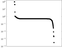
Figure 7: An equilateral triangle $\Gamma_{2}$ (left) and the spectrum of the discretized linear system for $\Gamma_{2}$ (right)

Figure 8: A right angle triangle $\Gamma_{3}$ (left) and the spectrum of the discretized linear system for $\Gamma_{3}$ (right)

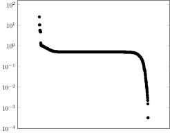
Figure 9: A star-shaped curve $\Gamma_{4}$ (left) and the spectrum of the discretized linear system for $\Gamma_{4}$ (right)

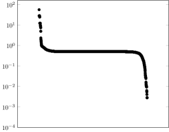
Figure 10: A tank-shaped curve $\Gamma_{5}$ (left) and the spectrum of the discretized linear system for $\Gamma_{5}$ (right)

Remark 45.

We note that the condition numbers reported for the boundaries $\Gamma_{j}$, $j=2,3,4,5$, are larger than the condition numbers of the underlying integral equations. This issue can be remedied by using a slightly more involved scaling of the discretization scheme (see, for example, [28]).

6 Conclusions and extensions

In this paper, we construct an explicit basis for the solution of a standard integral equation corresponding to the biharmonic equation with gradient boundary conditions, on polygonal domains. The explicit and detailed knowledge of the behavior of solutions to the integral equation in the vicinity of the corner was used to create purpose-made discretizations, resulting in efficient numerical schemes accurate to essentially machine precision. In this section, we discuss several directions in which these results are generalizable.

6.1 Infinite oscillations of the biharmonic Green’s function

In 1973, S. Osher showed that the domain Green’s function for the biharmonic equation has infinite oscillations for a right-angled wedge, and conjectured that this result holds for any domain with corners. Earlier, we observed that the representations of solutions to the associated integral equations also exhibit infinite oscillations near the corner (see Remark 37). The oscillatory behavior of these basis functions suggests that Osher’s conjecture may be amenable to an analysis similar to the one presented in this paper.

6.2 Curved boundaries

In this paper, we derive a representation for the solutions of the integral equations associated with the biharmonic equation, on polygonal domains. In the more general case of curved boundaries with corners, the apparatus of this paper also leads to detailed representations of the solutions near corners. Specifically, the solutions to the associated integral equations are representable by rapidly convergent series of products of complex powers of $t$ and logarithms of $t$, where $t$ is the distance from the corner. This analysis closely mirrors the generalization of the authors’ analysis of Laplace’s equation on polygonal domains (see [17]) to the authors’ analysis on domains having curved boundaries with corners (see [29]).

6.3 Generalization to three dimensions

The apparatus of this paper admits a straightforward generalization to surfaces with edge singularities, where the parts of the surface on either side of the edge meet at a constant angle along on the edge. The generalization to the case of edges with more complicated geometries is more involved and will be presented at a later date.

6.4 Other boundary conditions

In this paper, we analyze the integral equations associated with the velocity boundary value problem for Stokes equation. The approach of this paper extends to a number of other boundary conditions, including the traction boundary value problem, and the mobility problem. In particular, the traction boundary value problem and the mobility problem can be formulated as boundary integral equations that are the adjoints of the integral equations for the velocity boundary value problem.

6.5 Modified biharmonic equation

The modified biharmonic equation for a potential $\psi$ is given by $\Delta^{2}\psi-\alpha\Delta\psi=0$. The equation naturally arises when mixed implicit-explicit schemes are used for the time discretization of the incompressible Navier-Stokes equation (see, for example [30]). A preliminary analysis indicates that the solutions of the integral equations associated with the modified biharmonic equation are representable as rapidly convergent series of Bessel functions of certain non-integer complex orders. The generalization of the analysis of the biharmonic equation, presented in this paper, to the analysis of the modified biharmonic equation closely mirrors the generalization of the authors’ analysis of Laplace’s equation (see [17]) to the authors’ analysis of the Helmholtz equation (see [19]).

7 Acknowledgements

The authors would like to thank Philip Greengard, Leslie Greengard, Jeremy Hoskins, Vladimir Rokhlin, and Jon Wilkening for many useful discussions.

M. Rachh’s work was supported in part by the Office of Naval Research award number N00014-14-1-0797/16-1-2123 and by AFOSR award number FA9550-16-1-0175. K. Serkh’s work was supported in part by the NSF Mathematical Sciences Postdoctoral Research Fellowship (award number 1606262) and by AFOSR award number FA9550-16-1-0175.

8 Appendix A

In this appendix, we prove theorems 27, 39 which are restated here as theorems 75, and 76, respectively. Section 8.1 deals with the tangential odd, normal even case (see 99), and Section 8.2 deals with the tangential even, normal odd case (see 100).

8.1 Tangential odd, normal even case

Suppose that ${\mathbf{A}}(z,\theta)$ is the $2\times 2$ matrix defined in 111. We recall that

$$\det{{\mathbf{A}}(z,\theta)}=\frac{\left(z\sin{(\pi\theta)}-\sin{(\pi z\theta)}\right)\left(z\sin{(\pi\theta)}-\sin{(\pi z(2-\theta))}\right)}{4\sin^{2}{(\pi z)}}\,.$$ (184)

If $z$ is not an integer, and satisfies either

$$z\sin{(\pi\theta)}-\sin{(\pi z(2-\theta))}=0,$$ (185)

or

$$z\sin{(\pi\theta)}-\sin{(\pi z\theta)}=0\,,$$ (186)

then $\det{({\mathbf{A}}(z,\theta))}=0$. Section 8.1.1 deals with the implicit functions defined by 185 and, similarly, Section 8.1.2 deals with the implicit functions defined by 186. The principal result of this section is Theorem 75, which is a restatement of Theorem 27.

8.1.1 Analysis of implicit function $z$ in 185

Suppose that $H:{\mathbb{C}}\times{\mathbb{C}}\to{\mathbb{C}}$ is the entire function defined by

$$H(z,\theta)=z\sin{(\pi\theta)}-\sin{(\pi z(2-\theta))}\,.$$ (187)

In this section, we investigate the implicit functions $z(\theta)$ which satisfy $H(z(\theta),\theta)=0$.

We begin by stating the connection between $\mathrm{sinc}{(z)}$ and the function $H(z,\theta)$ defined in 187.

Lemma 46.

Suppose that $G:{\mathbb{C}}\times{\mathbb{C}}\to{\mathbb{C}}$ is the entire function defined by

$$G(w,\alpha)=\mathrm{sinc}{(w)}+\mathrm{sinc}{(\alpha)}\,.$$ (188)

Then $G(w,\alpha)=0$ if and only if $H(z,\theta)=0$ where $z=\frac{w}{\alpha}$ and $\theta=2-\frac{\alpha}{\pi}$.

Proof. Since $z=\frac{w}{\alpha}$ and $\theta=2-\frac{\alpha}{\pi}$.

$$H(z,\theta)=z\sin{(\pi\theta)}-\sin{(\pi z(2-\theta))} =0\quad\iff$$ (189)

$$-z\sin{(\pi(2-\theta))}-\sin{(\pi z(2-\theta))} =0\quad\iff$$ (190)

$$\frac{w}{\alpha}\sin{(\alpha)}+\sin{w} =0\quad\iff$$ (191)

$$G(w,\alpha) =0\,.$$ (192)

$\blacksquare$

A simple calculation shows that

$$\frac{d}{dz}\mathrm{sinc}{(z)}=\tan{(z)}-z\,.$$ (193)

In the following lemma, we discuss the zeros of $\tan{(z)}-z$.

Lemma 47.

There exists a countable collection of real $\lambda_{j}>0$, $j=1,2,\ldots$ such that all the zeros of $\tan{(z)}-z$ are given by $\{-\lambda_{j}\}_{j=1}^{\infty}\cup\{\lambda_{j}\}_{j=1}^{\infty}\cup\{0\}$, where $\lambda_{j}\in(j\pi+\frac{\pi}{4},j\pi+\frac{\pi}{2})$.

Proof. We first show that all the zeros of $\tan{(z)}-z$ are real. We observe that, if $z=x+iy$, then

$$\tan{(z)}=\frac{\sin{(2x)}}{\cos{(2x)}+\cosh{(2y)}}+i\frac{\sinh{(2y)}}{\cos{(2x)}+\cosh{(2y)}}\,,$$ (194)

If $\tan{z}=z$, then

$$\frac{\sin{(2x)}}{2x}=\frac{\sinh{(2y)}}{2y}\,.$$ (195)

For all $y\neq 0$, $|\frac{\sinh{(2y)}}{2y}|>1$ and for all $x$, $|\frac{\sin{(2x)}}{2x}|\leq 1$. Thus, if $\tan{(z)}-z=0$, then $z\in{\mathbb{R}}$.

Next, we observe that $x=0$ clearly satisfies $\tan{(x)}=x$. Furthermore, we note that if $\lambda\in{\mathbb{R}}$ satifies $\tan{(\lambda)}=\lambda$, then $-\lambda$ also satisfies $\tan{(-\lambda)}=-\lambda$ since since $\tan{(x)}$ is an odd function of $x$. Thus, we restrict our attention to the roots of $\tan{(x)}=x$ for $x>0$. There are no roots of $\tan{(x)}=x$ on the intervals $(j\pi+\pi/2,(j+1)\pi]$, $j=0,1,2\ldots$, since $\tan{(x)}<0$ for all $x\in(j\pi+\pi/2,(j+1)\pi)$, $j=0,1,2\ldots$. Moreover, for all $j\geq 1$, there are no roots of $\tan{(x)}=x$ on the intervals $[j\pi,j\pi+\pi/4]$, since $0\leq\tan{(x)}\leq 1$ for $x\in[j\pi,j\pi+\pi/4]$ , and $x>1$ on $[j\pi,j\pi+\pi/4]$.

Figure 11: The solutions $\lambda_{1}$, $\lambda_{2}$ of $\tan{(x)}=x$.

Also, there are no roots of $\tan{(x)}=x$ for $x\in(0,\pi/2)$, since $\frac{d}{dx}\tan{(x)}>1$ for all $x\in(0,\pi/2)$. Finally, for each $j=1,2,\ldots$, $\tan{(x)}:(j\pi+\pi/4,j\pi+\pi/2)\to(1,\infty)$ is a bijection. Thus, there exists exactly one value $\lambda_{j}\in(j\pi+\pi/4,j\pi+\pi/2)$ such that $\tan{(x)}=x$. $\blacksquare$

The following lemma describes some elementary properties of $\lambda_{j}$, $j=1,2,\ldots\infty$.

Lemma 48.

Suppose that $\lambda_{j}$ are as defined in Lemma 47. Then

• $\mathrm{sinc}{(\lambda_{j})}=\cos{(\lambda_{j})}$

• $\cos{(\lambda_{2j})}>0$, $j=1,2,\ldots$, and $\cos{(\lambda_{2j-1})}<0$, $j=1,2,\ldots$

• $|\cos{(\lambda_{j})}|>|\cos{(\lambda_{j+1})}|$

Proof. Recall that $\lambda_{j}$, satisfy $\tan{(\lambda_{j})}=\lambda_{j}$. Thus,

$$\mathrm{sinc}{(\lambda_{j})}=\frac{\sin{(\lambda_{j})}}{\lambda_{j}}=\frac{\tan{(\lambda_{j})}\cos{(\lambda_{j})}}{\lambda_{j}}=\cos{(\lambda_{j})}\,.$$ (196)

Since $\lambda_{j}\in(j\pi+\pi/4,j\pi+\pi/2)$, $j=1,2,\ldots$, it follows that $\cos{(\lambda_{2n})}>0$ and $\cos{(\lambda_{2n-1})}<0$.

Finally, suppose $\lambda_{j}=j\pi+\theta_{j}$, where $\theta_{j}\in(\pi/4,\pi/2)$, $j=1,2,\ldots$. We first show that $\theta_{j+1}>\theta_{j}$. We note that $\tan{(\lambda_{j})}=\tan{(\theta_{j}+j\pi)}=\tan{(\theta_{j})}$. Thus,

$$\tan{(\theta_{j+1})}=\lambda_{j+1}>\lambda_{j}=\tan{(\theta_{j})}\,.$$ (197)

Since, $\tan{(\theta)}$ is a strictly monotonically increasing function for $\theta\in(0,\pi/2)$, we conclude that $\theta_{j+1}>\theta_{j}$. Then, $|\cos{(\lambda_{j})}|=|\cos{(j\pi+\theta_{j})}|=\cos{(\theta_{j})}$. Since $\cos{(\theta)}$ is a strictly monotonically decreasing function for $\theta\in(0,\pi/2)$, we conclude that $|\cos{(\lambda_{j})}|=\cos{(\theta_{j})}>\cos{(\theta_{j+1})}=|\cos{(\lambda_{j+1})}|$, $j=1,2,\ldots$. $\blacksquare$

In the following lemma, we describe contours in the complex plane for which $\mathrm{sinc}{(z)}$ is a real number.

Lemma 49.

Suppose that $j$ is a positive integer and that $\lambda_{j}$ is defined in Lemma 47. Then there exists a function $x_{j}:{\mathbb{R}}\to(j\pi,\lambda_{j}]$ which satisfies

$$x_{j}(y)=\tan{(x_{j}(y))}\cdot y\cdot\coth{(y)}\,,\quad x_{j}(0)=\lambda_{j}\,,$$ (198)

for all $y\in{\mathbb{R}}$. Furthermore, if $z=x_{j}(y)+iy$, then $\mathrm{sinc}{(z)}\in{\mathbb{R}}$.

Proof. It suffices to show existence of the function $x_{j}(y)$ which satisfies 198 for $y\geq 0$, since if $(x_{j}(y),y)$ satisfies 198, then $(x_{j}(-y),-y)$ also satisfies 198, i.e. the function $x_{j}(y)$ defined for $y\in[0,\infty)$ can be extended to $y\in(-\infty,\infty)$ using an even extension.

We observe that $y\coth{y}:[0,\infty)\to[1,\infty)$ is a strictly monotically increasing function and a bijection. Furthermore, an argument similar to the proof of Lemma 47 shows that for each $m\in[1,\infty)$, there exists a unique solution $x_{j}$ of the equation $x/m=\tan{(x)}$ contained in the interval $(j\pi,\lambda_{j}]$. Moreover, the mapping from $m\to x_{j}$ is monotonically decreasing as a function of $m$ and maps $m\in[1,\infty)\to x_{j}\in(j\pi,\lambda_{j}]$ (see Figure 12). Combining both of these statements, it follows that there exists a unique $x_{j}(y)$ for each $y$ which satisfies 198 and moreover, $x_{j}(y):[0,\infty)\to(j\pi,\lambda_{j}]$ is a bijection.

Figure 12: An illustrative figure to demonstrate the solutions $x_{1}(m)$ and $x_{2}(m)$ of $\tan{(x)}=x/m$ as a function of $m$.

Finally, a simple calculation shows that, if $z=x+iy$, then

$$\mathrm{sinc}{(z)}=\frac{1}{x^{2}+y^{2}}(x\sin{(x)}\cosh{(y)}+y\cos{(x)}\sinh{(y)}+i(x\cos{(x)}\sinh{(y)}-y\sin{(x)}\cosh{(y)}))\,,$$ (199)

from which it follows that $\mathrm{sinc}{(x_{j}(y)+iy)}$ is real for all $y\in{\mathbb{R}}$. $\blacksquare$

In the following lemma, we describe the behavior of the $\mathrm{sinc}$ function along the curve $(x_{j}(y),y)$, $j=1,2\ldots$.

Lemma 50.

Suppose that $j$ is a positive integer. Suppose $x_{j}:{\mathbb{R}}\to(j\pi,\lambda_{j}]$ is as defined in Lemma 49. Suppose further that $z_{j}:{\mathbb{R}}\to{\mathbb{C}}$ is defined by $z_{j}(y)=x_{j}(y)+iy$. Then the following holds

• Case 1, $j$ is even: $\mathrm{sinc}{(z_{j}(y))}$ is a strictly monotonically increasing function of $y$ for all $y>0$, and $\mathrm{sinc}{(z_{j}(y))}:(0,\infty)\to(\cos{(\lambda_{j})},\infty)$ is a bijection. Likewise, $\mathrm{sinc}{(z_{j}(y))}$ is a strictly monotonically decreasing function of $y$ for all $y<0$, and $\mathrm{sinc}{(z_{j}(y))}:(-\infty,0)\to(\cos{(\lambda_{j})},\infty)$ is a bijection.

• Case 2, $j$ is odd: $\mathrm{sinc}{(z_{j}(y))}$ is a strictly monotonically decreasing function of $y$ for all $y>0$, and $\mathrm{sinc}{(z_{j}(y))}:(0,\infty)\to(-\infty,\cos{(\lambda_{j})})$ is a bijection. Likewise, $\mathrm{sinc}{(z_{j}(y))}$ is a strictly monotonically decreasing function of $y$ for all $y<0$, and $\mathrm{sinc}{(z_{j}(y))}:(-\infty,0)\to(-\infty,\cos{(\lambda_{j})})$ is a bijection.

Proof. We prove the result for the case when $j$ is even. The proof for the case when $j$ is odd follows in a similar manner.

A simple calculation shows that

$$\mathrm{sinc}{(z_{j}(y))}=\frac{\cos{(x_{j}(y))}\sinh{(y)}}{y}$$ (200)

Recall that $x_{j}(y)=x_{j}(-y)$, and hence, $\mathrm{sinc}{(z_{j}(y))}=\mathrm{sinc}{(z_{j}(-y))}$. Thus, it suffices to prove the result when $y>0$.

Using Lemma 47, we note that $d/dz(\mathrm{sinc}{(z_{j}(y))})\neq 0$ for all $y>0$. Hence for every $z_{j}(y)$, there exists a $\delta>0$ such that $\mathrm{sinc}{(z)}$ is one-one for all $z\in|z-z_{j}(y)|<\delta$. It then follows that $\mathrm{sinc}{(z_{j}(y))}$ is either a strictly monotonically increasing function or a strictly monotonically decreasing function for all $y>0$.

When $j$ is even, using 200 and that $\lim_{y\to\infty}x_{j}(y)=j\pi$, we conclude that $\lim_{y\to\infty}\mathrm{sinc}{(z_{j}(y))}=\infty$. Finally, from Lemmas 49 and 48, we note that $\mathrm{sinc}{(z_{j}(0))}=\mathrm{sinc}{(\lambda_{j})}=\cos{(\lambda_{j})}$. Thus, $\mathrm{sinc}{(z_{j}(y))}$ is a strictly monotonically increasing function and $\mathrm{sinc}{(z_{j}(y))}:(0,\infty)\to(\cos{(\lambda_{j})},\infty)$ is a bijection. $\blacksquare$

We note that $x(y)=0$ satisfies 198 for all $y\in{\mathbb{R}}$. Moreover, if $z=x(y)+iy=iy$, we note that $\mathrm{sinc}{(z)}$ is real. Thus, it is natural to define $x_{0}(y)\equiv 0$ for all $y$.

In the following lemma, we discuss the inverse of $\mathrm{sinc}{(z)}$.

Lemma 51.

Suppose that $j$ is a positive integer. Suppose $x_{j}(y)$, $j=1,2,\ldots$ for $y\in{\mathbb{R}}$, are as defined in Lemma 49. Suppose further that we define $x_{0}(y)=0$ for all $y\in{\mathbb{R}}$. Let $\mathbb{H}^{+}$ denote the upper half plane and $\mathbb{H}^{-}$ denote the lower half plane. Furthermore, for any set $A\subset{\mathbb{C}}$, we denote the closure of $A$ by $\overline{A}$. Suppose $\Gamma_{j,+}$ is the open set in the upper half plane bounded by the curves $x_{j}(y)$ and $x_{j+1}(y)$, i.e.

$$\Gamma_{j,+}=\{(x,y):x_{j}(y)<x<x_{j+1}(y)\,,\quad\text{and}\quad y>0\}\,,$$ (201)

for $j=0,1,2,\ldots$ (see Figure 13). Similarly suppose that $\Gamma_{j,-}$ is the open set in the lower half plane bounded by the curves $x_{j}(y)$ and $x_{j+1}(y)$, i.e.

$$\Gamma_{j,-}=\{(x,y):x_{j}(y)<x<x_{j+1}(y)\,,\quad\text{and}\quad y<0\}\,,$$ (202)

for $j=1,2,\ldots$ (see Figure 13). Then the following holds.

• Case 1, $j$ is even: $\mathrm{sinc}{(z)}:\overline{\Gamma}_{j,+}\to\overline{\mathbb{H}}^{-}$ is a bijection which maps $\Gamma_{j,+}\to{\mathbb{R}}$. Moreover, the inverse function, which we denote by $\mathrm{sinc}^{-1}_{j,+}(z)$, is a bijection from $\overline{\mathbb{H}}^{-}\to\overline{\Gamma}_{j,+}$ and is analytic for $z\in\mathbb{H}^{-}$. Similarly, $\mathrm{sinc}{(z)}:\overline{\Gamma}_{j,-}\to\overline{\mathbb{H}}^{+}$ is a bijection which maps $\Gamma_{j,-}\to{\mathbb{R}}$. The inverse function, which we denote by $\mathrm{sinc}^{-1}_{j,-}(z)$, is a bijection from $\overline{\mathbb{H}}^{+}\to\overline{\Gamma}_{j,-}$ and is analytic for $z\in\mathbb{H}^{+}$.

• Case 2, $j$ is odd: $\mathrm{sinc}{(z)}:\overline{\Gamma}_{j,+}\to\overline{\mathbb{H}}^{+}$ is a bijection which maps $\Gamma_{j,+}\to{\mathbb{R}}$. Moreover, the inverse function, which we denote by $\mathrm{sinc}^{-1}_{j,+}(z)$, is a bijection from $\overline{\mathbb{H}}^{+}\to\overline{\Gamma}_{j,+}$ and is analytic for $z\in\mathbb{H}^{+}$. Similarly, $\mathrm{sinc}{(z)}:\overline{\Gamma}_{j,-}\to\overline{\mathbb{H}}^{-}$ is a bijection which maps $\Gamma_{j,-}\to{\mathbb{R}}$. The inverse function, which we denote by $\mathrm{sinc}^{-1}_{j,-}(z)$, is a bijection from $\overline{\mathbb{H}}^{-}\to\overline{\Gamma}_{j,-}$ and is analytic for $z\in\mathbb{H}^{-}$.

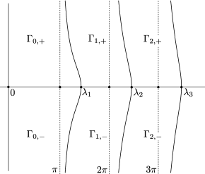
Figure 13: The regions $\Gamma_{j,+}$ and $\Gamma_{j,-}$ $j=0,1,2\ldots$

Proof. We prove the result for the case $\mathrm{sinc}{(z)}:\overline{\Gamma}_{j,+}\to\overline{\mathbb{H}}^{-}$, when $j$ is even. The results for the other cases follows in a similar manner. First, it follows from Lemma 47 that $\frac{d}{dz}\mathrm{sinc}{(z)}\neq 0$ for all $z\in\Gamma_{j,+}$ Thus, $\mathrm{sinc}{(z)}$ is conformal for $z\in\Gamma_{j,+}$. Using Lemma 50, we note that $\mathrm{sinc}{(z)}:\partial\Gamma_{j,+}\to{\mathbb{R}}$ is a bijection. Thus, $\mathrm{sinc}{(z)}$ either maps $\Gamma_{j,+}$ to either the lower half plane or the upper half plane. A simple calculation shows that when $j$ is even, $\mathrm{sinc}{(z)}$ maps $\Gamma_{j,+}$ to the lower half plane. Since $\mathrm{sinc}{(z)}$ is conformal for $z\in\Gamma_{j,+}$, the inverse $\mathrm{sinc}^{-1}_{j,+}(z)$ exists, is a bijection from $\overline{\mathbb{H}}^{-}\to\overline{\Gamma}_{j,+}$ and is analytic for $z\in\mathbb{H}^{-}$. $\blacksquare$

In the following lemma, we discuss the solutions $\alpha\in[0,2\pi]$ of $\mathrm{sinc}{(\alpha)}=-\cos{(\lambda_{j})}$.

Lemma 52.

Suppose $j$ is a positive integer and $\lambda_{j}$ is defined in Lemma 47.

• Case 1, $j$ is even: the equation $\mathrm{sinc}{(\alpha)}=-\cos{(\lambda_{j})}$ has only two solutions $\alpha^{j}_{1}$, and $\alpha^{j}_{2}$ on the interval $\alpha\in[0,2\pi]$ where $\pi<\alpha^{j}_{1}<\lambda_{1}<\alpha^{j}_{2}<2\pi$.

• Case 2, $j$ is odd: the equation $\mathrm{sinc}{(\alpha)}=-\cos{(\lambda_{j})}$ has only one solution $\alpha^{j}_{1}$ on the interval $\alpha\in[0,2\pi]$, where $0<\alpha^{j}_{1}<\pi$.

Proof. Suppose that $j$ is even. We note that $-\cos{(\lambda_{j})}<0$ and furthermore $-\cos{(\lambda_{j})}>-\cos{(\lambda_{1})}$ (see Lemma 48). Firstly, we note that $\mathrm{sinc}{(\alpha)}\geq 0$ for all $\alpha\in[0,\pi]$. Thus, there are no solutions to $\mathrm{sinc}{(\alpha)}=-\cos{(\lambda_{j})}$ for $\alpha\in[0,\pi]$. Refering to Figure 14, we observe that $\mathrm{sinc}{(\alpha)}:(\pi,\lambda_{1})\to(-\cos{(\lambda_{1})},0)$ is a bijection. Thus, there exists a unique $\alpha^{j}_{1}\in(\pi,\lambda_{1})$ such that $\mathrm{sinc}{(\alpha^{j}_{1})}=-\cos{(\lambda_{j})}$. Similarly, $\mathrm{sinc}{(\alpha)}:(\lambda_{1},2\pi)\to(-\cos{(\lambda_{1})},0)$ is also a bijection. Thus, there exists a unique $\alpha^{j}_{2}\in(\lambda_{1},2\pi)$ such that $\mathrm{sinc}{(\alpha^{j}_{2})}=-\cos{(\lambda_{j})}$.

Suppose now that $j$ is odd. We note that $-\cos{(\lambda_{j})}>0$ (see Lemma 48). $\mathrm{sinc}{(\alpha)}\leq 0$ for $\alpha\in[\pi,2\pi]$. Thus, there are no solutions to $\mathrm{sinc}{(\alpha)}=-\cos{(\lambda_{j})}$ for $\alpha\in[\pi,2\pi]$. Finally, referring to Figure 14, we observe that $\mathrm{sinc}{(\alpha)}:(0,\pi)\to(0,1)$ is a bijection. Thus, there exists a unique $\alpha^{j}_{1}\in(0,\pi)$ such that $\mathrm{sinc}{(\alpha^{j}_{1})}=-\cos{(\lambda_{j})}$. $\blacksquare$

Figure 14: Solutions of $\mathrm{sinc}{(\alpha)}=-\cos{(\lambda_{j})}$. Case 1, $j$ is even ($-\cos{(\lambda_{j})}<0$) (left), and case 2, $j$ is odd ($-\cos{(\lambda_{j})}>0$) (right).

Even case, $z(1)=2m$ In this section, we analyze the implicit functions $z(\theta)$ which satisfy $H(z,\theta)=0$, with $z(1)=2m$ where $m$ is a positive integer. The principal result of this section is Lemma 56.

Lemma 53.

Suppose that $m$ is a positive integer, and that $G(w,\alpha)$ is as defined in 188. Suppose the regions $\Gamma_{j,+},\Gamma_{j,-}$, $j=0,1,\ldots$ are as defined in Lemma 51. Suppose that $\alpha^{2m-1}_{1}$, $\alpha^{2m}_{1}$, and $\alpha^{2m}_{2}$ are as defined in Lemma 52. As before, for any set $A$ let $\overline{A}$ denote the closure of $A$. Furthermore, suppose that $D$ is the strip in the lower half plane with $0<\text{Re}(\alpha)<2\pi$, i.e.

$$D=\{\alpha\in{\mathbb{C}}:\,0<\text{Re}(\alpha)<2\pi\,,\quad\text{Im}(\alpha)<0\}\,.$$ (203)

Suppose that $D_{1}$ is the region $\overline{D}\cap\overline{\Gamma}_{0,-}$ and $D_{2}$ is the region $\overline{D}\setminus\overline{\Gamma}_{0,-}$ (see Figure 15).

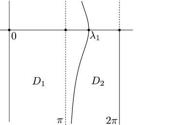
Figure 15: The regions $D_{1}=\overline{D}\cap\overline{\Gamma}_{0,-}$ and $D_{2}=\overline{D}\setminus\overline{\Gamma}_{0,-}$.

Suppose finally that $w(\alpha):\overline{D}\to{\mathbb{C}}$ is defined by

$$w(\alpha)=\begin{cases}\mathrm{sinc}^{-1}_{2m-1,-}(-\mathrm{sinc}{(\alpha)})&\quad\alpha\in D_{1}\\ \mathrm{sinc}^{-1}_{2m,-}(-\mathrm{sinc}{(\alpha)})&\quad\alpha\in D_{2}\,.\end{cases}$$ (204)

Then for all $\alpha\in D$, $w(\alpha)$ satisfies $G(w(\alpha),\alpha)=0$ and is an analytic function for $\alpha\in D$. Moreover, $w(\pi)=2m\pi$.

Proof. Suppose, as before, that $\mathbb{H}^{+}$ denotes the upper half plane and $\mathbb{H}^{-}$ denotes the lower half plane. We first note that for all $\alpha\in\overline{D}$, the function $w$ is well defined and satisfies $G(w(\alpha),\alpha)=0$. For $\alpha\in D_{1}$, $w(\alpha)=\mathrm{sinc}^{-1}_{2m-1,-}(-\mathrm{sinc}{(\alpha)})$. The domain of definition for for $\mathrm{sinc}^{-1}_{2m-1,-}(z)$ is $z\in\overline{\mathbb{H}}^{+}$, and using Lemma 51, $-\mathrm{sinc}{(\alpha)}\in\overline{\mathbb{H}}^{+}$ for $\alpha\in D_{1}$. Moreover, for $\alpha\in\overline{D}_{1}$,

$$G(w(\alpha),\alpha) =\mathrm{sinc}{(w(\alpha))}+\mathrm{sinc}{(\alpha)}$$ (205)

$$=\mathrm{sinc}{(\mathrm{sinc}^{-1}_{2m-1,-}(-\mathrm{sinc}{(\alpha)})}+\mathrm{sinc}{(\alpha)}$$ (206)

$$=-\mathrm{sinc}{(\alpha)}+\mathrm{sinc}{(\alpha)}=0\,.$$ (207)

Similarly, for $\alpha\in D_{2}$, $w(\alpha)=\mathrm{sinc}^{-1}_{2m,-}(-\mathrm{sinc}{(\alpha)})$. The domain of definition for $\mathrm{sinc}^{-1}_{2m,-}(z)$ is $z\in\overline{\mathbb{H}}^{-}$, and using Lemma 51, $-\mathrm{sinc}{(\alpha)}\in\overline{\mathbb{H}}^{-}$ for all $\alpha\in D_{2}$. Moreover, for $\alpha\in\overline{D}_{2}$,

$$G(w(\alpha),\alpha) =\mathrm{sinc}{(w(\alpha))}+\mathrm{sinc}{(\alpha)}$$ (208)

$$=\mathrm{sinc}{(\mathrm{sinc}^{-1}_{2m,-}(-\mathrm{sinc}{(\alpha)})}+\mathrm{sinc}{(\alpha)}$$ (209)

$$=-\mathrm{sinc}{(\alpha)}+\mathrm{sinc}{(\alpha)}=0\,.$$ (210)

Clearly, $w(\alpha)$ is analytic for $\alpha\in D_{1}\cap D$ since both $\mathrm{sinc}^{-1}_{2m-1,-}(z)$ and $\mathrm{sinc}{(z)}$ are analytic functions on their respective domains of definition. Similarly, $w(\alpha)$ is analytic for $\alpha\in D_{2}\cap D$. In order to show that $w(\alpha)$ is analytic for $\alpha\in D$, it suffices to show that $w$ is continuous across $\overline{D}_{1}\cap\overline{D}_{2}$. It follows from the defintions of the regions $D_{1},D_{2}$, that $\overline{D}_{1}\cap\overline{D}_{2}$ is precisely the curve $(x_{1}(y),y)$ for $y\in(-\infty,0]$. For each $y\in(-\infty,0)$, let $\alpha(y)=x_{1}(y)+iy$. Then

$$\{-\mathrm{sinc}(\alpha(y))\,:\quad-\infty<y<0\}=(-\cos{(\lambda_{1})},\infty)\,.$$ (211)

Let $w(y)=x_{2m}(y)+iy$, for $y\in(-\infty,0)$, then $\mathrm{sinc}{(w(y))}\in(\cos{(\lambda_{2m})},\infty)$. Moreover, $\mathrm{sinc}{(w(y))}$ is a monotonically decreasing function of $y$ for $y<0$ (see Lemma 50). Furthermore, using Lemma 48, we note that $-\cos{(\lambda_{1})}>\cos{(\lambda_{2m})}$. Thus, there exists a unique $y_{1}\in(-\infty,0)$ such that $\mathrm{sinc}{(w(y_{1}))}=-\cos{(\lambda_{1})}$.

Referring to Figure 16(b), we observe that

$$\{\mathrm{sinc}^{-1}_{2m-1,-}{(y)}\,:\quad-\cos{(\lambda_{1})}<y<\infty\}=\{x_{2m}(y)+iy\,,\quad-\infty<y<y_{1}\}\,.$$ (212)

Similarly,

$$\{\mathrm{sinc}^{-1}_{2m,-}{(y)}\,:\quad-\cos{(\lambda_{1})}<y<\infty\}=\{x_{2m}(y)+iy\,,\quad-\infty<y<y_{1}\}\,.$$ (213)

Combining 211, 212 and 213, we conclude that $w(\alpha)$ is continuous across $\overline{D}_{1}\cap\overline{D}_{2}$. It then follows from Morera’s theorem that $w(\alpha)$ is analytic for $\alpha\in D$.

Finally $\pi\in D_{1}$, and it follows from the definition of $\mathrm{sinc}^{-1}_{2m-1,-}(z)$, that

$$w(\pi)=\mathrm{sinc}^{-1}_{2m-1,-}(-\mathrm{sinc}{(\pi)})=\mathrm{sinc}^{-1}_{2m-1,-}(0)=2m\pi\,,$$ (214)

from which the result follows. $\blacksquare$

Remark 54.

In Figure 16(b), we provide a more detailed description of the values of $w(\alpha)\in{\mathbb{C}}$, which satisfies $G(w(\alpha),\alpha)=0$ and $w(\pi)=2m\pi$, for $\alpha\in(0,2\pi)$.

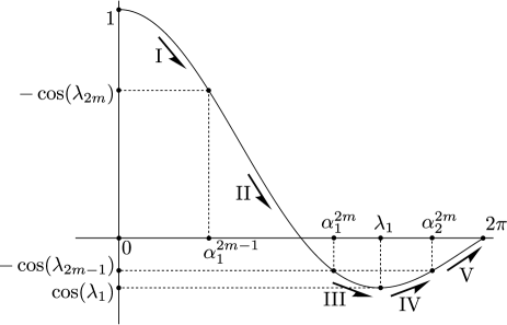
(a) The values of $\mathrm{sinc}{(\alpha)}$ for $\alpha\in(0,2\pi)$

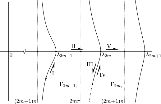
(b) The corresponding values of $w(\alpha)$ which satisfy $G(w(\alpha),\alpha)=0$ with $w(\pi)=2m\pi$

Figure 16: The values $\mathrm{sinc}{(\alpha)}$ for $\alpha\in(0,2\pi)$ (Figure 16(a)) and the corresponding values of $w(\alpha)$ which satisfy $G(w(\alpha),\alpha)=0$ with $w(\pi)=2m\pi$ (Figure 16(b)). In Figure 16(b), segment I represents $w(\alpha)$ for $\alpha\in(0,\alpha^{2m-1}_{1})$, segment II represents $w(\alpha)$ for $\alpha\in(\alpha^{2m-1}_{1},\alpha^{2m}_{1})$, segment III represents $w(\alpha)$ for $\alpha\in(\alpha^{2m}_{1},\lambda_{1})$, segment IV represents $w(\alpha)$ for $\alpha\in(\lambda_{1},\alpha^{2m}_{2})$, and finally segment V represents $w(\alpha)$ for $\alpha\in(\alpha^{2m}_{2},2\pi)$.

.

In the following lemma, we further extend the domain of definition of $w(\alpha)$ defined in Lemma 53 to a simply connected open set containing the strip in the lower half plane with $0<\text{Re}(\alpha)<2\pi$ that includes the interval $(0,2\pi)\setminus\{\alpha^{2m-1}_{1},\alpha^{2m}_{1},\alpha^{2m}_{2}\}$.

Lemma 55.

Suppose that $m$ is a positive integer, and that $G(w,\alpha)$ is as defined in 188. Suppose that $\alpha^{2m-1}_{1}$, $\alpha^{2m}_{1}$, and $\alpha^{2m}_{2}$ are as defined in Lemma 52. As before, let $\overline{A}$ denote the closure of the set $A$. Furthermore, suppose that the region $D$ and the analytic function $w(\alpha):\overline{D}\to{\mathbb{C}}$ is as defined in Lemma 53. Suppose now that $\tilde{D}$ is the strip in the lower half plane with $0<\text{Re}(\alpha)<2\pi$ that includes the interval $(0,2\pi)\setminus\{\alpha^{2m-1}_{1},\alpha^{2m}_{1},\alpha^{2m}_{2}\}$, i.e.,

$$\tilde{D}=\{\alpha\in{\mathbb{C}}:\,0<\text{Re}(\alpha)<2\pi\,,\quad\text{Im}(\alpha)\geq 0\}\setminus\{\alpha^{2m-1}_{1},\alpha^{2m}_{1},\alpha^{2m}_{2}\}\,.$$ (215)

Then there exists a simply connected open set $\tilde{D}\subset\tilde{V}\subset{\mathbb{C}}$ (see Figure 17 and an analytic function $\tilde{w}(\alpha):\tilde{V}\to{\mathbb{C}}$ which satisfies $G(\tilde{w}(\alpha),\alpha)=0$ for all $\alpha\in\tilde{V}$ and $\tilde{w}(\pi)=2m\pi$. Moreover $\tilde{w}(\alpha)=w(\alpha)$ for all $\alpha\in\overline{D}\cap\tilde{V}$.

Figure 17: An illustrative region of analyticity $\tilde{V}$ of the function $w(\alpha)$, which satisfies $G(w(\alpha),\alpha)=0$.

Proof. For all $\alpha\in\overline{D}\cap\tilde{V}$, we define $\tilde{w}(\alpha)=w(\alpha)$. We also note that the interval $(0,2\pi)\setminus\{\alpha^{2m-1}_{1},\alpha^{2m}_{1},\alpha^{2m}_{2}\}\subset\overline{D}\cap\tilde{V}$. Furthermore, $\tilde{w}(\alpha)$ also satisfies $G(\tilde{w}(\alpha),\alpha)=0$ for all $\alpha\in\overline{D}\cap\tilde{V}$, since $w(\alpha)$ satisfies $G(w(\alpha),\alpha)=0$. A simple calculation shows that $\partial_{w}G(\tilde{w}(\alpha),\alpha)=\tan{(\tilde{w}(\alpha))}-w(\alpha)$. Moreover, it follows from the definition of $\tilde{w}(\alpha)$ that $\tilde{w}(\alpha)\neq\lambda_{j}$, $j=1,2,\ldots$ for all $\alpha\in(0,2\pi)\setminus\{\alpha^{2m-1}_{1},\alpha^{2m}_{1},\alpha^{2m}_{2}\}$. Thus, we conclude from Lemma 47 that $\partial_{w}G(\tilde{w}(\alpha_{0}),\alpha_{0})\neq 0$ for each $\alpha_{0}\in(0,2\pi)\setminus\{\alpha^{2m-1}_{1},\alpha^{2m}_{1},\alpha^{2m}_{2}\}$. Finally, by the implicit function theorem there exists a $\delta>0$ and an implicit function $\tilde{w}(\alpha):|\alpha-\alpha_{0}|\to{\mathbb{C}}$ which satisfies $G(\tilde{w}(\alpha),\alpha)=0$, from which the result follows. $\blacksquare$

We now present the principal result of this section.

Lemma 56.

Suppose that $m$ is a positive integer and that $H(z,\theta)$ is as defined in 187. Suppose that $\alpha^{2m-1}_{1}$, $\alpha^{2m}_{1}$, and $\alpha^{2m}_{2}$ are as defined in Lemma 52. Suppose that $\theta_{1},\theta_{2}$, and $\theta_{3}$ are given by

$$\theta_{1}=2-\frac{\alpha^{2m}_{2}}{\pi}\,,\quad\theta_{2}=2-\frac{\alpha^{2m}_{1}}{\pi}\,,\quad\theta_{3}=2-\frac{\alpha^{2m-1}_{1}}{\pi}\,.$$ (216)

Suppose further that $D$ is the strip in the upper half plane with $0<\text{Re}(\theta)<2$ that includes the interval $(0,2)\setminus\{\theta_{1},\theta_{2},\theta_{3}\}$, i.e.

$$D=\{\theta\in{\mathbb{C}}:\,0<\text{Re}(\theta)<2\,,\quad\text{Im}(\theta)\geq 0\}\setminus\{\theta_{1},\theta_{2},\theta_{3}\}\,.$$ (217)

Then there exists a simply connected open set $D\subset V\subset{\mathbb{C}}$ (see Figure 18) and an analytic function $z(\theta):V\to{\mathbb{C}}$ which satisfies $H(z(\theta),\theta)=0$ for all $\theta\in V$ and $z(1)=2m$.

Figure 18: An illustrative region of analyticity $V$ of the function $z(\theta)$, which satisfies $H(z(\theta),\theta)=0$.

Proof. Suppose that $\tilde{V}$ and $\tilde{w}(\alpha):\tilde{V}\to{\mathbb{C}}$ are as defined in Lemma 55. Recall that $\tilde{V}$ is an open set containing the strip $\tilde{D}$ defined in 215. Let

$$\theta=2-\frac{\alpha}{\pi}\,,\quad z(\theta)=\frac{w((2-\theta)\pi)}{\pi(2-\theta)}\,,\quad\text{and}\quad V=2-\frac{\tilde{V}}{\pi}\,.$$ (218)

For all $\alpha\in\tilde{V}$, we note that $\theta\in V$. Furthermore, $\tilde{w}(\pi)=2m\pi$ implies that $z(1)=2m$. Finally, using Lemma 46, we conclude that $z(\theta)$ satisfies $H(z(\theta),\theta)=0$. $\blacksquare$

Remark 57.

Using the Taylor expansion of $\mathrm{sinc}{(\alpha)}$ in the neighborhood of $\alpha^{2m-1}_{1}$, $\alpha^{2m}_{1}$ and $\alpha^{2m}_{2}$, it is straightforward to show that $w(\alpha)$ in Lemma 53 has square root singularities at $\alpha=\alpha^{2m-1}_{1},\alpha^{2m}_{1},\alpha^{2m}_{2}$. It then follows from the definition of $z(\theta)$ in Lemma 56 has square root singularities at $\theta=\theta_{1},\theta_{2}$, and $\theta_{3}$. Thus, $\theta_{1},\theta_{2}$, and $\theta_{3}$ are branch points for the function $z(\theta)$.

Odd case, $z(1)=2m-1$, $m\neq 1$ In this section, we analyze the implicit functions which satisfy $H(z,\theta)=0$, with $z(1)=2m-1$, where $m\geq 2$ is an integer. The principal result of this section is Lemma 60. The proofs of the results presented in this section are analogous to the corresponding proofs in Figure 14. We present the statements of the theorem without proofs for brevity.

In the following lemma, we construct an analytic function $w(\alpha)$ which satisfies $G(w(\alpha),\alpha)=0$ with $w(1)=(2m-1)\pi$.

Lemma 58.

Suppose that $m\geq 2$ is an integer, and that $G(w,\alpha)$ is as defined in 188. Suppose the regions $\Gamma_{j,+},\Gamma_{j,-}$, $j=0,1,\ldots$ are as defined in Lemma 51. Suppose that $\alpha^{2m-1}_{1}$, $\alpha^{2m-2}_{1}$, and $\alpha^{2m-2}_{2}$ are as defined in Lemma 52. As before, let $\overline{A}$ denote the closure of the set $A$. Furthermore, suppose that $D$ is the strip in the lower half plane with $0<\text{Re}(\alpha)<2\pi$, i.e.

$$D=\{\alpha\in{\mathbb{C}}:\,0<\text{Re}(\alpha)<2\pi\,,\quad\text{Im}(\alpha)<0\}\,.$$ (219)

Suppose that $D_{1}$ is the region $\overline{D}\cap\overline{\Gamma}_{0,-}$ and $D_{2}$ is the region $\overline{D}\setminus D_{1}$. Suppose finally that $w(\alpha):\overline{D}\to{\mathbb{C}}$ is defined by

$$w(\alpha)=\begin{cases}\mathrm{sinc}^{-1}_{2m-2,+}(-\mathrm{sinc}{(\alpha)})&\quad\alpha\in D_{1}\\ \mathrm{sinc}^{-1}_{2m-3,+}(-\mathrm{sinc}{(\alpha)})&\quad\alpha\in D_{2}\,.\end{cases}$$ (220)

Then for all $\alpha\in D$, $w(\alpha)$ satisfies $G(w(\alpha),\alpha)=0$ and is an analytic function for $\alpha\in D$. Moreover, $w(\pi)=(2m-1)\pi$.

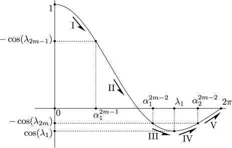
(a) The values $\mathrm{sinc}{(\alpha)}$ for $\alpha\in(0,2\pi)$

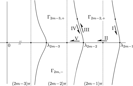
(b) The corresponding values of $w(\alpha)$ which satisfy $G(w(\alpha),\alpha)=0$ with $w(\pi)=(2m-1)\pi$

Figure 19: The values $\mathrm{sinc}{(\alpha)}$ for $\alpha\in(0,2\pi)$ (Figure 19(a)) and the corresponding values of $w(\alpha)$ which satisfy $G(w(\alpha),\alpha)=0$ with $w(\pi)=(2m-1)\pi$ (Figure 19(b)). In Figure 19(b), segment I represents $w(\alpha)$ for $\alpha\in(0,\alpha^{2m-1}_{1})$, segment II represents $w(\alpha)$ for $\alpha\in(\alpha^{2m-1}_{1},\alpha^{2m-2}_{1})$, segment III represents $w(\alpha)$ for $\alpha\in(\alpha^{2m-2}_{1},\lambda_{1})$, segment IV represents $w(\alpha)$ for $\alpha\in(\lambda_{1},\alpha^{2m-2}_{2})$, and finally segment V represents $w(\alpha)$ for $\alpha\in(\alpha^{2m-2}_{2},2\pi)$.

Remark 59.

Referring to Figure 19, we provide a detailed description for the behavior of $w(\alpha)$ defined in Lemma 58 for $\alpha\in(0,2\pi)$.

We present the principal result of this section in the following lemma.

Lemma 60.

Suppose that $m\geq 2$ is an integer and that $H(z,\theta)$ is as defined in 187. Suppose that $\alpha^{2m-1}_{1}$, $\alpha^{2m-2}_{1}$, and $\alpha^{2m-2}_{2}$ are as defined in Lemma 52. Suppose that $\theta_{1},\theta_{2}$, and $\theta_{3}$ are given by

$$\theta_{3}=2-\frac{\alpha^{2m-2}_{2}}{\pi}\,,\quad\theta_{2}=2-\frac{\alpha^{2m-2}_{1}}{\pi}\,,\quad\theta_{1}=2-\frac{\alpha^{2m-1}_{1}}{\pi}\,.$$ (221)

Suppose further that $D$ is the strip in the upper half plane with $0<\text{Re}(\theta)<2$ that includes the interval $(0,2)\setminus\{\theta_{1},\theta_{2},\theta_{3}\}$, i.e.

$$D=\{\theta\in{\mathbb{C}}:\,0<\text{Re}(\theta)<2\,,\quad\text{Im}(\theta)\geq 0\}\setminus\{\theta_{1},\theta_{2},\theta_{3}\}\,.$$ (222)

Then there exists a simply connected open set $D\subset V\subset{\mathbb{C}}$ and an analytic function $z(\theta):V\to{\mathbb{C}}$ which satisfies $H(z(\theta),\theta)=0$ for all $\theta\in V$ and $z(1)=2m-1$.

Odd case, $z(1)=1$ In this section, we analyze the implicit functions which satisfy $H(z,\theta)=0$, with $z(1)=1$. The principal result of this section is Lemma 63. The proofs of the results presented in this section are analogous to the corresponding proofs in Figure 14. We present the statements of the theorem without proofs for brevity.

In the following lemma, we construct an analytic function $w(\alpha)$ which satisfies $G(w(\alpha),\alpha)=0$ with $w(1)=\pi$.

Lemma 61.

Suppose that $G(w,\alpha)$ is as defined in 188. Suppose the regions $\Gamma_{0,+},\Gamma_{0,-}$ are as defined in Lemma 51. Suppose that $\alpha^{1}_{1}$ is as defined in Lemma 52. As before, let $\overline{A}$ denote the closure of the set $A$. Furthermore, suppose that $D$ is the strip in the lower half plane with $0<\text{Re}(\alpha)<2\pi$, i.e.

$$D=\{\alpha\in{\mathbb{C}}:\,0<\text{Re}(\alpha)<2\pi\,,\quad\text{Im}(\alpha)<0\}\,.$$ (223)

Suppose that $D_{1}$ is the region $\overline{D}\cap\overline{\Gamma}_{0,-}$ and $D_{2}$ is the region $\overline{D}\setminus D_{1}$. Suppose finally that $w(\alpha):\overline{D}\to{\mathbb{C}}$ is defined by

$$w(\alpha)=\begin{cases}\mathrm{sinc}^{-1}_{0,+}(-\mathrm{sinc}{(\alpha)})&\quad\alpha\in D_{1}\\ \mathrm{sinc}^{-1}_{0,-}(-\mathrm{sinc}{(\alpha)})&\quad\alpha\in D_{2}\,.\end{cases}$$ (224)

Then for all $\alpha\in D$, $w(\alpha)$ satisfies $G(w(\alpha),\alpha)=0$ and is an analytic function for $\alpha\in D$. Moreover, $w(\pi)=\pi$.

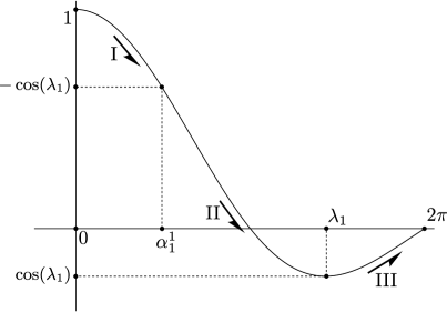
(a) The values $\mathrm{sinc}{(\alpha)}$ for $\alpha\in(0,2\pi)$

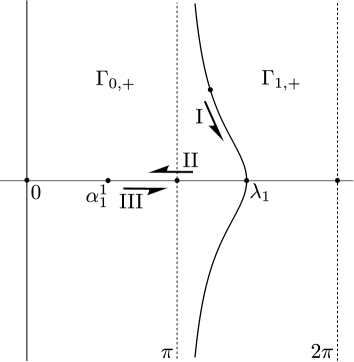
(b) The corresponding values of $w(\alpha)$ which satisfy $G(w(\alpha),\alpha)=0$ with $w(\pi)=\pi$

Figure 20: The values $\mathrm{sinc}{(\alpha)}$ for $\alpha\in(0,2\pi)$ (Figure 20(a)) and the corresponding values of $w(\alpha)$ which satisfy $G(w(\alpha),\alpha)=0$ with $w(\pi)=\pi$ (Figure 20(a)). In Figure 20(b), segment I represents $w(\alpha)$ for $\alpha\in(0,\alpha^{2m-1}_{1})$, segment II represents $w(\alpha)$ for $\alpha\in(\alpha^{2m-1}_{1},\alpha^{2m-2}_{1})$, and finally segment III represents $w(\alpha)$ for $\alpha\in(\alpha^{2m-2}_{1},\lambda_{1})$

Remark 62.

Referring to Figure 20, we provide a detailed description for the behavior of $w(\alpha)$ defined in Lemma 61 for $\alpha\in(0,2\pi)$.

We present the principal result of this section in the following lemma.

Lemma 63.

Suppose that $H(z,\theta)$ is as defined in 187. Suppose that $\alpha^{1}_{1}$ is as defined in Lemma 52. Furthermore, suppose that $\theta_{1}$ are given by

$$\theta_{1}=2-\frac{\alpha^{1}_{1}}{\pi}\,,$$ (225)

Suppose further that $D$ is the strip in the upper half plane with $0<\text{Re}(\theta)<2$ that includes the interval $(0,2)\setminus\{\theta_{1}\}$, i.e.

$$D=\{\theta\in{\mathbb{C}}:\,0<\text{Re}(\theta)<2\,,\quad\text{Im}(\theta)\geq 0\}\setminus\{\theta_{1}\}\,.$$ (226)

Then there exists a simply connected open set $D\subset V\subset{\mathbb{C}}$ (see Figure 21) and an analytic function $z(\theta):V\to{\mathbb{C}}$ which satisfies $H(z(\theta),\theta)=0$ for all $\theta\in V$ and $z(1)=1$.

Figure 21: An illustrative region of analyticity $V$ of the function $z(\theta)$, which satisfies $H(z(\theta),\theta)=0$ with $z(1)=1$.

8.1.2 Analysis of implicit function $z$ in 186

In this section, we investigate the implicit functions which satisfy

$$H(z,\theta)=z\sin{(\pi\theta)}-\sin{(\pi z\theta)}=0\,.$$ (227)

The analysis for the implicit functions $z(\theta)$ which satisfy $H(z,\theta)=0$ is similar to the analysis of the analogous implicit functions in Section 8.1.1. For conciseness, we present the statements of the theorems in this section and omit the proofs.

We first state the connection between $\mathrm{sinc}{(z)}$ and the function $H(z,\theta)$ defined in 227.

Lemma 64.

Suppose that $G:{\mathbb{C}}\times{\mathbb{C}}\to{\mathbb{C}}$ is the entire function defined by

$$G(w,\alpha)=\mathrm{sinc}{(w)}-\mathrm{sinc}{(\alpha)}\,.$$ (228)

Then $G(w,\alpha)=0$ if and only if $H(z,\theta)=0$ where $z=\frac{w}{\alpha}$ and $\theta=\frac{\alpha}{\pi}$.

In the following lemma, we discuss the solutions $\alpha\in[0,2\pi]$ of $\mathrm{sinc}{(\alpha)}=\cos{(\lambda_{j})}$.

Lemma 65.

Suppose $j$ is a positive integer and $\lambda_{j}$ is defined in Lemma 47.

• Case 1, $j$ is even: the equation $\mathrm{sinc}{(\alpha)}=\cos{(\lambda_{j})}$ has only one solution $\beta^{j}_{1}$ on the interval $\alpha\in[0,2\pi]$ where $0<\beta^{j}_{1}<\pi$ (see Figure 22).

• Case 2, $j$ is odd: the equation $\mathrm{sinc}{(\alpha)}=-\cos{(\lambda_{j})}$ has only two solutions $\beta^{j}_{1}$, and $\beta^{j}_{2}$ on the interval $\alpha\in[0,2\pi]$, where $\pi<\beta^{j}_{1}<\lambda_{1}<\beta^{j}_{2}<2\pi$ (see Figure 22).

Figure 22: Solutions of $\mathrm{sinc}{(\alpha)}=\cos{(\lambda_{j})}$. Case 1, $j$ is even ($\cos{(\lambda_{j})}>0$) (left), and case 2, $j$ is odd ($\cos{(\lambda_{j})}<0$) (right).

As before, the analysis of the implicit functions $w(\alpha)$ which satisfy $G(w,\alpha)=0$ (see 228), and the analogous functions $z(\theta)$ which satisfy $H(z,\theta)$ (see 227), is split into three cases. In Figure 22, we analyze the functions implicit functions $z(\theta)$ for the case $z(1)=2m-1$, where $m$ is a positive integer, in Lemma 68, we analyze the implicit functions $z(\theta)$ for the case $z(1)=2m$, where $m\geq 2$ is an integer, and finally in Lemma 71, we analyze the implicit function $z(\theta)$ for the case $z(1)=2$.

Odd case, $z(1)=2m-1$ In this section, we analyze the implicit functions which satisfy $H(z,\theta)=0$, with $z(1)=2m-1$, where $m$ is a positive integer. The principal result of this section is Lemma 68.

In the following lemma, we construct an analytic function $w(\alpha)$ which satisfies $G(w(\alpha),\alpha)=0$ with $w(1)=(2m-1)\pi$.

Lemma 66.

Suppose that $m$ is a positive integer, and that $G(w,\alpha)$ is as defined in 228. Suppose the regions $\Gamma_{j,+},\Gamma_{j,-}$, $j=0,1,\ldots$ are as defined in Lemma 51. Suppose that $\beta^{2m-2}_{1}$, $\beta^{2m-1}_{1}$, and $\beta^{2m-1}_{2}$ are as defined in Lemma 65. As before, let $\overline{A}$ denote the closure of the set $A$. Furthermore, suppose that $D$ is the strip in the upper half plane with $0<\text{Re}(\alpha)<2\pi$, i.e.

$$D=\{\alpha\in{\mathbb{C}}:\,0<\text{Re}(\alpha)<2\pi\,,\quad\text{Im}(\alpha)>0\}\,.$$ (229)

Suppose that $D_{1}$ is the region $\overline{D}\cap\overline{\Gamma}_{0,+}$ and $D_{2}$ is the region $\overline{D}\setminus\overline{\Gamma}_{0,+}$ (see Figure 23).

Figure 23: The regions $D_{1}=\overline{D}\cap\overline{\Gamma}_{0,+}$ and $D_{2}=\overline{D}\setminus\overline{\Gamma}_{0,+}$.

Suppose finally that $w(\alpha):\overline{D}\to{\mathbb{C}}$ is defined by

$$w(\alpha)=\begin{cases}\mathrm{sinc}^{-1}_{2m-2,-}(\mathrm{sinc}{(\alpha)})&\quad\alpha\in D_{1}\\ \mathrm{sinc}^{-1}_{2m-1,-}(\mathrm{sinc}{(\alpha)})&\quad\alpha\in D_{2}\,.\end{cases}$$ (230)

Then for all $\alpha\in D$, $w(\alpha)$ satisfies $G(w(\alpha),\alpha)=0$ and is an analytic function for $\alpha\in D$. Moreover, $w(\pi)=(2m-1)\pi$.

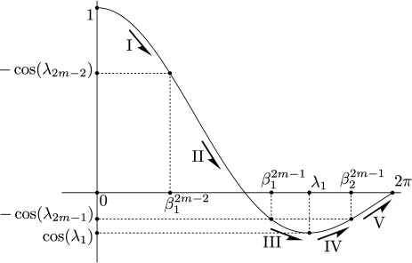
(a) The values $\mathrm{sinc}{(\alpha)}$ for $\alpha\in(0,2\pi)$

(b) The corresponding values of $w(\alpha)$ which satisfy $G(w(\alpha),\alpha)=0$ with $w(\pi)=(2m-1)\pi$

Figure 24: The values $\mathrm{sinc}{(\alpha)}$ for $\alpha\in(0,2\pi)$ (Figure 24(a)) and the corresponding values of $w(\alpha)$ which satisfy $G(w(\alpha),\alpha)=0$ with $w(\pi)=(2m-1)\pi$ (Figure 24(b)). In Figure 24(b), segment I represents $w(\alpha)$ for $\alpha\in(0,\beta^{2m-2}_{1})$, segment II represents $w(\alpha)$ for $\alpha\in(\beta^{2m-2}_{1},\beta^{2m-1}_{1})$, segment III represents $w(\alpha)$ for $\alpha\in(\beta^{2m-1}_{1},\lambda_{1})$, segment IV represents $w(\alpha)$ for $\alpha\in(\lambda_{1},\beta^{2m-1}_{2})$, and finally segment V represents $w(\alpha)$ for $\alpha\in(\beta^{2m-1}_{2},2\pi)$.

Remark 67.

Referring to Figure 24, we provide a detailed description for the behavior of $w(\alpha)$ defined in Lemma 66 for $\alpha\in(0,2\pi)$.

We present the principal result of this section in the following lemma.

Lemma 68.

Suppose that $m$ is a positive integer and that $H(z,\theta)$ is as defined in 227. Suppose that $\beta^{2m-2}_{1}$, $\beta^{2m-1}_{1}$, and $\beta^{2m-1}_{2}$ are as defined in Lemma 65. Suppose that $\theta_{1},\theta_{2}$, and $\theta_{3}$ are given by

$$\theta_{1}=\frac{\beta^{2m-2}_{1}}{\pi}\,,\quad\theta_{2}=\frac{\beta^{2m-1}_{1}}{\pi}\,,\quad\theta_{3}=\frac{\beta^{2m-1}_{2}}{\pi}\,.$$ (231)

Suppose further that $D$ is the strip in the upper half plane with $0<\text{Re}(\theta)<2$ that includes the interval $(0,2)\setminus\{\theta_{1},\theta_{2},\theta_{3}\}$, i.e.

$$D=\{\theta\in{\mathbb{C}}:\,0<\text{Re}(\theta)<2\,,\quad\text{Im}(\theta)\geq 0\}\setminus\{\theta_{1},\theta_{2},\theta_{3}\}\,.$$ (232)

Then there exists a simply connected open set $D\subset V\subset{\mathbb{C}}$ and an analytic function $z(\theta):V\to{\mathbb{C}}$ which satisfies $H(z(\theta),\theta)=0$ for all $\theta\in V$ and $z(1)=2m-1$.

Even case, $z(1)=2m$, $m\neq 1$ In this section, we analyze the implicit functions which satisfy $H(z,\theta)=0$, with $z(1)=2m$, where $m\geq 2$ is an integer. The principal result of this section is Lemma 71.

In the following lemma, we construct an analytic function $w(\alpha)$ which satisfies $G(w(\alpha),\alpha)=0$ with $w(1)=2m\pi$.

Lemma 69.

Suppose that $m\geq 2$ is an integer, and that $G(w,\alpha)$ is as defined in 228. Suppose the regions $\Gamma_{j,+},\Gamma_{j,-}$, $j=0,1,\ldots$ are as defined in Lemma 51. Suppose that $\beta^{2m}_{1}$, $\beta^{2m-1}_{1}$, and $\beta^{2m-1}_{2}$ are as defined in Lemma 65. As before, let $\overline{A}$ denote the closure of the set $A$. Furthermore, suppose that $D$ is the strip in the upper half plane with $0<\text{Re}(\alpha)<2\pi$, i.e.

$$D=\{\alpha\in{\mathbb{C}}:\,0<\text{Re}(\alpha)<2\pi\,,\quad\text{Im}(\alpha)>0\}\,.$$ (233)

Suppose that $D_{1}$ is the region $\overline{D}\cap\overline{\Gamma}_{0,+}$ and $D_{2}$ is the region $\overline{D}\setminus D_{1}$ (see Figure 23). Suppose finally that $w(\alpha):\overline{D}\to{\mathbb{C}}$ is defined by

$$w(\alpha)=\begin{cases}\mathrm{sinc}^{-1}_{2m-1,+}(\mathrm{sinc}{(\alpha)})&\quad\alpha\in D_{1}\\ \mathrm{sinc}^{-1}_{2m-2,+}(\mathrm{sinc}{(\alpha)})&\quad\alpha\in D_{2}\,.\end{cases}$$ (234)

Then for all $\alpha\in D$, $w(\alpha)$ satisfies $G(w(\alpha),\alpha)=0$ and is an analytic function for $\alpha\in D$. Moreover, $w(\pi)=2m\pi$.

(a) The values $\mathrm{sinc}{(\alpha)}$ for $\alpha\in(0,2\pi)$

(b) The corresponding values of $w(\alpha)$ which satisfy $G(w(\alpha),\alpha)=0$ with $w(\pi)=2m\pi$

Figure 25: The values $\mathrm{sinc}{(\alpha)}$ for $\alpha\in(0,2\pi)$ (Figure 25(a)) and the corresponding values of $w(\alpha)$ which satisfy $G(w(\alpha),\alpha)=0$ with $w(\pi)=2m\pi$ (Figure 25(b)). In Figure 25(b), segment I represents $w(\alpha)$ for $\alpha\in(0,\beta^{2m}_{1})$, segment II represents $w(\alpha)$ for $\alpha\in(\beta^{2m}_{1},\beta^{2m-1}_{1})$, segment III represents $w(\alpha)$ for $\alpha\in(\beta^{2m-1}_{1},\lambda_{1})$, segment IV represents $w(\alpha)$ for $\alpha\in(\lambda_{1},\beta^{2m-1}_{2})$, and finally segment V represents $w(\alpha)$ for $\alpha\in(\beta^{2m-1}_{2},2\pi)$.

Remark 70.

Referring to Figure 25, we provide a detailed description for the behavior of $w(\alpha)$ defined in Lemma 69 for $\alpha\in(0,2\pi)$.

We present the principal result of this section in the following lemma.

Lemma 71.

Suppose that $m\geq 2$ is an integer and that $H(z,\theta)$ is as defined in 227. Suppose that $\beta^{2m}_{1}$, $\beta^{2m-1}_{1}$, and $\beta^{2m-1}_{2}$ are as defined in Lemma 65. Suppose that $\theta_{1},\theta_{2}$, and $\theta_{3}$ are given by

$$\theta_{1}=\frac{\beta^{2m}_{1}}{\pi}\,,\quad\theta_{2}=\frac{\beta^{2m-1}_{1}}{\pi}\,,\quad\theta_{3}=\frac{\beta^{2m-1}_{2}}{\pi}\,.$$ (235)

Suppose further that $D$ is the strip in the upper half plane with $0<\text{Re}(\theta)<2$ that includes the interval $(0,2)\setminus\{\theta_{1},\theta_{2},\theta_{3}\}$, i.e.

$$D=\{\theta\in{\mathbb{C}}:\,0<\text{Re}(\theta)<2\,,\quad\text{Im}(\theta)\geq 0\}\setminus\{\theta_{1},\theta_{2},\theta_{3}\}\,.$$ (236)

Then there exists a simply connected open set $D\subset V\subset{\mathbb{C}}$ and an analytic function $z(\theta):V\to{\mathbb{C}}$ which satisfies $H(z(\theta),\theta)=0$ for all $\theta\in V$ and $z(1)=2m$.

Even case, $z(1)=2$ In this section, we analyze the implicit functions which satisfy $H(z,\theta)=0$, with $z(1)=2$. The principal result of this section is Lemma 74.

In the following lemma, we construct an analytic function $w(\alpha)$ which satisfies $G(w(\alpha),\alpha)=0$ with $w(1)=2\pi$.

Lemma 72.

Suppose that $G(w,\alpha)$ is as defined in 228. Suppose the regions $\Gamma_{0,+},\Gamma_{0,-}$ are as defined in Lemma 51. Suppose that $\beta^{2}_{1}$ is as defined in Lemma 65. As before, let $\overline{A}$ denote the closure of the set $A$. Furthermore, suppose that $D$ is the strip in the upper half plane with $0<\text{Re}(\alpha)<2\pi$, i.e.

$$D=\{\alpha\in{\mathbb{C}}:\,0<\text{Re}(\alpha)<2\pi\,,\quad\text{Im}(\alpha)>0\}\,.$$ (237)

Suppose that $D_{1}$ is the region $\overline{D}\cap\overline{\Gamma}_{0,+}$ and $D_{2}$ is the region $\overline{D}\setminus D_{1}$. Suppose finally that $w(\alpha):\overline{D}\to{\mathbb{C}}$ is defined by

$$w(\alpha)=\begin{cases}\mathrm{sinc}^{-1}_{1,+}(\mathrm{sinc}{(\alpha)})&\quad\alpha\in D_{1}\\ \mathrm{sinc}^{-1}_{0,+}(\mathrm{sinc}{(\alpha)})&\quad\alpha\in D_{2}\,.\end{cases}$$ (238)

Then for all $\alpha\in D$, $w(\alpha)$ satisfies $G(w(\alpha),\alpha)=0$ and is an analytic function for $\alpha\in D$. Moreover, $w(\pi)=2\pi$.

(a) The values $\mathrm{sinc}{(\alpha)}$ for $\alpha\in(0,2\pi)$

(b) The corresponding values of $w(\alpha)$ which satisfy $G(w(\alpha),\alpha)=0$ with $w(\pi)=2\pi$

Figure 26: The values $\mathrm{sinc}{(\alpha)}$ for $\alpha\in(0,2\pi)$ (Figure 26(a)) and the corresponding values of $w(\alpha)$ which satisfy $G(w(\alpha),\alpha)=0$ with $w(\pi)=2\pi$ (Figure 26(b)). In Figure 26(b), segment I represents $w(\alpha)$ for $\alpha\in(0,\beta^{2}_{1})$, segment II represents $w(\alpha)$ for $\alpha\in(\beta^{2}_{1},\lambda_{1})$, and finally segment III represents $w(\alpha)$ for $\alpha\in(\lambda_{1},2\pi)$.

Remark 73.

Referring to Figure 26, we provide a detailed description for the behavior of $w(\alpha)$ defined in Lemma 72 for $\alpha\in(0,2\pi)$.

We present the principal result of this section in the following lemma.

Lemma 74.

Suppose that $H(z,\theta)$ is as defined in 227. Suppose that $\beta^{2}_{1}$ is as defined in Lemma 65. Furthermore, suppose that $\theta_{1}$ is given by

$$\theta_{1}=\frac{\beta^{2}_{1}}{\pi}\,,$$ (239)

Suppose further that $D$ is the strip in the upper half plane with $0<\text{Re}(\theta)<2$ that includes the interval $(0,2)\setminus\{\theta_{1}\}$, i.e.

$$D=\{\theta\in{\mathbb{C}}:\,0<\text{Re}(\theta)<2\,,\quad\text{Im}(\theta)\geq 0\}\setminus\{\theta_{1}\}\,.$$ (240)

Then there exists a simply connected open set $D\subset V\subset{\mathbb{C}}$ and an analytic function $z(\theta):V\to{\mathbb{C}}$ which satisfies $H(z(\theta),\theta)=0$ for all $\theta\in V$ and $z(1)=2$.

Finally, we now present the principal result of Section 8.1.

Theorem 75.

Suppose that $N\geq 2$ is an integer. Then there exists $3N-2$ real numbers $\theta_{1},\theta_{2},\ldots\theta_{3N-2}\in(0,2)$ such that the following holds. Suppose that $D$ is the strip in the upper half plane with $0<\text{Re}(\theta)<2$ that includes the interval $(0,2)\setminus\{\theta_{j}\}_{j=1}^{3N-2}$, i.e.

$$D=\{\theta\in{\mathbb{C}}\,:\,\text{Re}(\theta)\in(0,2)\,,\quad 0\leq\text{Im}(\theta)<\infty\}\setminus\{\theta_{j}\}_{j=1}^{3N-2}\,.$$ (241)

Then, there exists a simply connected open set $D\subset V\subset{\mathbb{C}}$ and analytic functions $z_{n,1}(\theta):V\to{\mathbb{C}}$, $n=1,2\ldots N$, which satisfy

$$z\sin{(\pi\theta)}-\sin{(\pi z(2-\theta))}=0\,,\quad z(1)=n\,,$$ (242)

for $\theta\in V$, and analytic functions $z_{n,2}(\theta):V\to{\mathbb{C}}$, $n=2,3,\ldots N$, which satisfy

$$z\sin{(\pi\theta)}-\sin{(\pi z\theta)}=0\,,\quad z(1)=n\,,$$ (243)

for $\theta\in V$ (see Figure 27 for an illustrative domain $V$). Moreover, the functions $z_{n,1}(\theta)$, $n=1,2\ldots N$, do not take integer values for all $\theta\in V\setminus\{1\}$, and satisfy $\det{{\mathbf{A}}(z_{n,1}(\theta),\theta)}=0$, $n=1,2\ldots N$, for all $\theta\in V$ (see 111 and 118). Similarly, the functions $z_{n,2}(\theta)$, $n=2,3,\ldots N$, do not take integer values for all $\theta\in V\setminus\{1\}$, and satisfy $\det{{\mathbf{A}}(z_{n,2}(\theta),\theta)}=0$, $n=2,3\ldots N$, for all $\theta\in V$ (see 111 and 118).

Figure 27: An illustrative domain $V$ for the case $N=2$, where $\theta_{1},\theta_{2},\ldots\theta_{5}$ are the combined branch points of the functions $z_{1,1}(\theta)$, $z_{2,1}(\theta)$, and $z_{2,2}(\theta)$. The large dashes are used to denote the interval $(0,2)$ for reference. The thin dashes are the locations of the branch cuts at $\theta_{1},\theta_{2}\ldots\theta_{5}$.

Proof. Suppose that $m$ is a positive integer. Let $z_{n,1}(\theta)$, $n=2m$, $n\leq N$, be the analytic functions defined in Lemma 56 and $V_{n,1}$, $n=2m$, $n\leq N$ be the regions of analyticity of $z_{n,1}(\theta)$. Similarly, let $z_{n,1}(\theta)$, $n=2m+1$, $n\leq N$, be the analytic functions defined in Lemma 60 and $V_{n,1}$, $n=2m+1$, $n\leq N$ be the regions of analyticity of $z_{n,1}(\theta)$. Let $z_{1,1}(\theta)$ be the analytic function defined in Lemma 63 and $V_{1,1}$ be the region of analyticity of $z_{1,1}(\theta)$. Proceeding in a similar manner, let $z_{n,2}(\theta)$, and $V_{n,2}$, $n=2,3\ldots N$, be the analytic functions and their domain of analyticity as defined in Lemmas 68, 71 and 74. Suppose that $\alpha^{j}_{1}$ and $\alpha^{j}_{2}$ are as defined in Lemma 52, and $\beta^{j}_{1}$ and $\beta^{j}_{2}$ are as defined in Lemma 65. Let $\theta_{1},\theta_{2},\ldots\theta_{3N-2}$ be the colletion of numbers

$$\left\{\theta_{j}\right\}_{j=1}^{3N-2}= \left\{2-\frac{\alpha^{2m-1}_{1}}{\pi}\right\}_{m=1}^{2m-1\leq N}\cup\left\{2-\frac{\alpha^{2m}_{1}}{\pi}\right\}_{m=1}^{2m\leq N}\cup\left\{2-\frac{\alpha^{2m}_{2}}{\pi}\right\}_{m=1}^{2m\leq N}\cup$$

$$\left\{\frac{\beta^{2m+1}_{1}}{\pi}\right\}_{m=1}^{2m+1\leq N}\cup\left\{\frac{\beta^{2m+1}_{1}}{\pi}\right\}_{m=1}^{2m+1\leq N}\cup\left\{\frac{\beta^{2m}_{2}}{\pi}\right\}_{m=1}^{2m\leq N}\,.$$ (244)

Clearly, $V=\cap_{n=1}^{N}V_{n,1}\cap_{n=2}^{N}V_{n,2}$ is a simply connected open neighborhood such that $D\subset V$ and $V$ is the common region of analyticity of the functions $z_{n,1}(\theta)$, $n=1,2,\ldots N$, and $z_{n,2}(\theta)$, $n=2,3,\ldots N$. Furthermore, it follows from Lemmas 56, 60, 63, 68, 71 and 74 that the domain $V$, the analytic functions $z_{n,1}(\theta)$, $n=1,2,\ldots N$, and the analytic functions $z_{n,2}(\theta)$, $n=2,3,\ldots N$, satisfy all the conditions of the theorem. $\blacksquare$

8.2 Tangential even, normal odd case

Suppose that ${\mathbf{A}}(z,\theta)$ is the $2\times 2$ matrix defined in 152. We recall that

$$\det{{\mathbf{A}}(z,\theta)}=\frac{\left(z\sin{(\pi\theta)}+\sin{(\pi z\theta)}\right)\left(z\sin{(\pi\theta)}+\sin{(\pi z(2-\theta))}\right)}{4\sin^{2}{(\pi z)}}\,.$$ (245)

If $z$ is not an integer, and satisfies either

$$z\sin{(\pi\theta)}+\sin{(\pi z(2-\theta))}=0,$$ (246)

or

$$z\sin{(\pi\theta)}+\sin{(\pi z\theta)}=0\,,$$ (247)

then $\det{({\mathbf{A}}(z,\theta)}=0$. The analysis of the implicit functions $z(\theta)$ which satisfy 246 and 247 for the tangential even, normal odd case is similar to the analysis of the implicit functions $z(\theta)$ which satisfy 185 and 186 for the tangential odd, normal even case. The principal result of this section is Theorem 76, which is a restatement of Theorem 39. For brevity, we omit the proof.

Theorem 76.

Suppose that $N\geq 2$ is an integer. Then there exists $3N-2$ real numbers $\theta_{1},\theta_{2},\ldots\theta_{3N-2}\in(0,2)$ such that the following holds. Suppose that $D$ is the strip in the upper half plane with $0<\text{Re}(\theta)<2$ that includes the interval $(0,2)\setminus\{\theta_{j}\}_{j=1}^{3N-2}$, i.e.

$$D=\{\theta\in{\mathbb{C}}\,:\,\text{Re}(\theta)\in(0,2)\,,\quad 0\leq\text{Im}(\theta)<\infty\}\setminus\{\theta_{j}\}_{j=1}^{3N-2}\,.$$ (248)

Then, there exists a simply connected open set $D\subset V\subset{\mathbb{C}}$ and analytic functions $z_{n,1}(\theta):V\to{\mathbb{C}}$, $n=2,3\ldots N$, which satisfy

$$z\sin{(\pi\theta)}+\sin{(\pi z(2-\theta))}=0\,,\quad z(1)=n\,,$$ (249)

for $\theta\in V$, and analytic functions $z_{n,2}(\theta):V\to{\mathbb{C}}$, $n=1,2,\ldots N$, which satisfy

$$z\sin{(\pi\theta)}+\sin{(\pi z\theta)}=0\,,\quad z(1)=n\,,$$ (250)

for $\theta\in V$ (see Figure 27 for an illustrative domain $V$). Moreover, the functions $z_{n,1}(\theta)$, $n=2,3\ldots N$, do not take integer values for all $\theta\in V\setminus\{1\}$, and satisfy $\det{{\mathbf{A}}(z_{n,1}(\theta),\theta)}=0$, $n=2,3\ldots N$, for all $\theta\in V$ (see 152 and 156). Similarly, the functions $z_{n,2}(\theta)$, $n=1,2,\ldots N$, do not take integer values for all $\theta\in V\setminus\{1\}$, and satisfy $\det{{\mathbf{A}}(z_{n,2}(\theta),\theta)}=0$, $n=1,2\ldots N$, for all $\theta\in V$ (see 152 and 156).

9 Appendix B

In this section we compute the limit $\theta\to 1$, of the linear transformation ${\mathbf{B}}(\theta)$, which maps coefficients of singular basis functions for the solution of the integral equation to the Taylor expansion coefficients of the velocity field. In Section 9.1, we investigate the tangential odd, normal even case (see 99) and, in Section 9.2, we investigate the tangential even, normal odd case (see 100).

9.1 Tangential odd, normal even case

Suppose that ${\mathbf{A}}(z,\theta)$ is the $2\times 2$ matrix given by 111 defined in Section 4.1. Suppose $N$ is a positive integer. Suppose further that, as in Theorem 27, $z_{n,1}(\theta)$, $n=1,2,\ldots N$, are analytic functions satisfying $\det{{\mathbf{A}}(z_{n,1}(\theta),\theta)}=0$ for $\theta\in V_{\delta}\subset{\mathbb{C}}$, where $V_{\delta}$ is a neighborhood of the contour $C_{\delta}$. Similarly, suppose that $z_{n,2}(\theta)$, $n=2,3\ldots N$, are analytic functions satisfying $\det{{\mathbf{A}}(z_{n,2}(\theta),\theta)}=0$ for $\theta\in V_{\delta}$. Let $(p_{n,1},q_{n,1})\in{\mathcal{N}}\{{\mathbf{A}}(z_{n,1}(\theta),\theta)\}$, $n=1,2,\ldots N$, and $(p_{n,2},q_{n,2})\in{\mathcal{N}}\{{\mathbf{A}}(z_{n,2}(\theta),\theta)\}$, $n=2,3,\ldots N$. We further assume that the vectors $(p_{n,1},q_{n,1})$, $n=1,2,\ldots$ and $(p_{n,2},q_{n,2})$, $n=2,3,\ldots$, are $\ell^{2}$ normalized. Suppose that $z_{1,2}(\theta)\equiv 1$, $p_{1,2}=0$, and $q_{1,2}=1$. Finally, suppose that ${\mathbf{B}}(\theta)$ is a $(2N+2)\times(2N+2)$ matrix defined in Theorem 32 for $\theta\in V_{\delta}$. The $2\times 2$ blocks of ${\mathbf{B}}(\theta)$ are given by

$${\mathbf{B}}_{\ell,n}(\theta)=\left[\begin{array}[]{c;{2pt/2pt}c}{\mathbf{F}}(\ell,z_{n,1}(\theta),\theta)\begin{bmatrix}p_{n,1}(\theta)\\ q_{n,1}(\theta)\end{bmatrix}&{\mathbf{F}}(\ell,z_{n,2}(\theta),\theta) \begin{bmatrix}p_{n,2}(\theta) \\ q_{n,2}(\theta) \end{bmatrix}\end{array}\right]\,,$$ (251)

for $\ell,n=1,2,\ldots N$, where ${\mathbf{F}}$ is defined in 114, except for the case $\ell=n=1$. In the case $\ell=n=1$, the matrix ${\mathbf{B}}_{1,1}(\theta)$ is given by

$${\mathbf{B}}_{1,1}(\theta)=\left[\begin{array}[]{c;{2pt/2pt}c}{\mathbf{F}}(1,z_{1,1}(\theta),\theta)\begin{bmatrix}p_{1,1}(\theta)\\ q_{1,1}(\theta)\end{bmatrix}&{\mathbf{F}}_{1}(\theta)\end{array}\right]\,,$$ (252)

where ${\mathbf{F}}$ is defined in 114, and ${\mathbf{F}}_{1}$ is defined in 128. Finally, if either $\ell=0$ or $n=0$, then the matrices ${\mathbf{B}}_{\ell,n}(\theta)$ are given by

$${\mathbf{B}}_{\ell,0}(\theta) =\begin{bmatrix}0&0\\ 0&0\end{bmatrix}\,,$$ (253)

$${\mathbf{B}}_{0,0}(\theta) ={\mathbf{F}}_{0}(\theta)\,,$$ (254)

$${\mathbf{B}}_{0,n}(\theta) ={\mathbf{F}}(n,0,\theta)\,,$$ (255)

for $\ell,n=1,2,\ldots N$, where ${\mathbf{F}}$ is defined in 114, and ${\mathbf{F}}_{0}$ is defined in 131.

In the following lemma, we describe the behavior of $z_{n,1}(\theta),p_{n,1}(\theta)$, and $q_{n,1}(\theta)$, $n=1,2,\ldots$, in the vicinity of $\theta=1$.

Lemma 77.

Suppose that $z_{n,1}(\theta)$, $n=1,2,\ldots$, satisfying $\det{{\mathbf{A}}(z_{n,1}(\theta),\theta)}=0$, be as defined in Theorem 27. Suppose further that $(p_{n,1}(\theta),q_{n,1}(\theta))$, $n=1,2,\ldots$, be an $\ell^{2}$ normalized null vector of ${\mathbf{A}}(z_{n,1},\theta)$. Then in the neighborhood of $\theta=1$,

$$z_{2n,1}(\theta) =2n-\frac{\pi^{2}n(4n^{2}-1)}{3}(\theta-1)^{3}+O(|\theta-1|^{4})$$ (256)

$$p_{2n,1}(\theta) =-\frac{\pi(2n-1)}{2}(\theta-1)+O(|\theta-1|^{3})$$ (257)

$$q_{2n,1}(\theta) =1+O(|\theta-1|^{2})$$ (258)

$$z_{2n+1,1}(\theta) =2n+1+2(2n+1)(\theta-1)+O(|\theta-1|^{2})$$ (259)

$$p_{2n+1,1}(\theta) =1+O(|\theta-1|)$$ (260)

$$q_{2n+1,1}(\theta) =O(|\theta-1|)\,.$$ (261)

Proof. Let the superscript ^′ denote derivative with respect to $\theta$ and $\partial_{t}$ denote the partial derivative with respect to $t$. Suppose that $H(z,\theta)$ is given by

$$H(z,\theta)=z\sin{(\pi\theta)}-\sin{(\pi z(2-\theta))}$$ (262)

From Theorem 27, we recall that $z_{n,1}(\theta)$, $n=1,2,\ldots$, satisfy $H(z_{n,1},\theta)=0$. Using the implicit function theorem

$$z^{\prime}(\theta)=-\frac{\partial_{\theta}H}{\partial_{z}H}=z(1-\sec{(\pi z)})$$ (263)

Thus,

$$z^{\prime}_{2n,1}(1)=0\,,\quad\text{and}\quad z^{\prime}_{2n+1,1}(1)=2(2n+1)\,.$$ (264)

Implicitly differentiating $H$ twice we get

$$\partial_{z}H\cdot z^{\prime\prime}(\theta)+\left(\frac{d}{d\theta}\partial_{z}H+\partial_{z}\partial_{\theta}H\right)\cdot z^{\prime}(\theta)+\partial_{\theta}\partial_{\theta}H=0\,.$$ (265)

Since $z_{2n,1}^{\prime}(1)=0$, we get

$$z_{2n,1}^{\prime\prime}(1)=-\frac{\partial_{\theta\theta}H}{\partial_{z}H}=\pi z^{2}\tan{(\pi z)}=0\,.$$ (266)

Proceeding in a similar fashion, we observe that

$$z_{2n,1}^{\prime\prime\prime}(1)=-\frac{\partial_{\theta\theta\theta}H}{\partial_{z}H}=\pi^{2}z_{2n,1}(\sec{(\pi z_{2n,1})}-z_{2n,1}^{2})=2\pi^{2}n(1-4n^{2})\,.$$ (267)

Let

$$\tilde{p}_{n,1}(\theta) =-\sin{(\pi z)}+2a_{2,2}(z_{n,1}(\theta),\theta)\,,$$ (268)

$$\tilde{q}_{n,1}(\theta) =2\sin{(\pi z)}a_{2,1}(z_{n,1}(\theta),\theta)\,,$$ (269)

where $a_{2,1}$ and $a_{2,2}$ are defined in 88 and 89 respectively. Clearly, $(\tilde{p}_{n,1},\tilde{q}_{n,1})\in{\mathcal{N}}({\mathbf{A}})$. We then set

$$p_{n,1}(\theta)=\frac{\tilde{p}_{n,1}}{\sqrt{(\tilde{p}_{n,1}^{2}+\tilde{q}_{n,1}^{2})}}\,,\quad\text{and}\quad q_{n,1}(\theta)=\frac{\tilde{q}_{n,1}}{\sqrt{(\tilde{p}_{n,1}^{2}+\tilde{q}_{n,1}^{2})}}$$ (270)

The required Taylor expansions for $p_{n,1},q_{n,1}$ are then readily obtained by using the Taylor expansions of $z_{n,1}(\theta)$. $\blacksquare$

In the next lemma, we now describe the behavior of $z_{n,2}(\theta),p_{n,2}(\theta)$ and $q_{n,2}(\theta)$, $n=2,3,\ldots$, in the vicinity of $\theta=1$.

Lemma 78.

Suppose that $z_{n,2}(\theta)$, $n=2,3,\ldots$, satisfying $\det{{\mathbf{A}}(z_{n,2}(\theta),\theta)}=0$, be as defined in Theorem 27. Suppose further that $(p_{n,2}(\theta),q_{n,2}(\theta))$, $n=2,3,\ldots$, be an $\ell^{2}$ normalized null vector of ${\mathbf{A}}(z_{n,2},\theta)$. Then in the neighborhood of $\theta=1$,

$$z_{2n,2}(\theta) =2n-4n(\theta-1)+O(|\theta-1|^{2})$$ (271)

$$p_{2n,2}(\theta) =1+O(|\theta-1|)$$ (272)

$$q_{2n,2}(\theta) =0+O(|\theta-1|)$$ (273)

$$z_{2n+1,1}(\theta) =2n+1+\frac{2\pi^{2}n(n+1)(2n+1)}{3}(\theta-1)^{3}+O(|\theta-1|^{4})$$ (274)

$$p_{2n+1,2}(\theta) =-\pi n(\theta-1)+O(|\theta-1|^{3})$$ (275)

$$q_{2n+1,2}(\theta) =1+O(|\theta-1|^{2})$$ (276)

Proof. The proof proceeds in a similar manner as the proof of Lemma 77. $\blacksquare$

Combining Lemmas 77 and 78, we present the principal result of this section, which computes the limit $\theta\to 1$ of the matrix ${\mathbf{B}}(\theta)$ in the following theorem.

Theorem 79.

Suppose that $N$ is a positive integer and suppose further that ${\mathbf{B}}$ is given by 251, 252, 253, 254 and 255. Then

$$\lim_{\theta\to 1}{\mathbf{B}}_{\ell,j}(\theta)=\begin{cases}\begin{bmatrix}-1/2&0\\ 0&-1/2\end{bmatrix}&\quad\ell=j=0\vspace*{3pt}\\ \begin{bmatrix}0&-1/2\\ -1/2&0\end{bmatrix}&\quad\ell=j=2m\neq 0\vspace*{3pt}\\ \begin{bmatrix}-1/2&0\\ 0&-1/2\end{bmatrix}&\quad\ell=j=2m+1\vspace*{3pt}\\ \begin{bmatrix}0&0\\ 0&0\end{bmatrix}&\quad\text{otherwise}\end{cases}\,,$$ (277)

for all $\ell,j=0,1,\ldots N$.

Proof. Let $\tilde{{\mathbf{F}}}(n,\theta)=2\pi{\mathbf{F}}(n,z,\theta)\cdot(n-z)$ for $j,\ell=1,2$ where ${\mathbf{F}}$ is given by 114. On inspecting the entries of $\tilde{{\mathbf{F}}}(n,\theta)$, we observe that

$$\tilde{{\mathbf{F}}}(n,1)=\begin{bmatrix}0&0\\ 0&0\end{bmatrix}\,,$$ (278)

for all $n\in{\mathbb{N}}$. Since $z_{j,\ell}(1)=j$, we conclude that

$$\lim_{\theta\to 1}{\mathbf{F}}(n,z_{j,\ell},\theta)\begin{bmatrix}p_{j,\ell}\\ q_{j,\ell}\end{bmatrix}=\lim_{\theta\to 1}\frac{\tilde{{\mathbf{F}}}(n,\theta)}{(-z_{j,\ell}+n)}\begin{bmatrix}p_{j,\ell}\\ q_{j,\ell}\end{bmatrix}=\begin{bmatrix}0\\ 0\end{bmatrix}\,,$$ (279)

for all $j\neq n$, and $\ell=1,2$. ${\mathbf{B}}_{n,0}(\theta)=0$ is the zero matrix by definition and for ${\mathbf{B}}_{0,n}(\theta)$, we have

$$\lim_{\theta\to 1}{\mathbf{B}}_{0,n}(\theta)=\lim_{\theta\to 1}{\mathbf{F}}(n,0,\theta)=\lim_{\theta\to 1}\frac{\tilde{{\mathbf{F}}}(n,\theta)}{2\pi n}=\begin{bmatrix}0&0\\ 0&0\end{bmatrix}\,,$$ (280)

for $n=1,2,\ldots N$.

We now turn our attention to the diagonal terms. For $n=0$, it follows from a simple calculation that

$$\lim_{\theta\to 1}{\mathbf{B}}_{0,0}(\theta)=\lim_{\theta\to 1}{\mathbf{F}}_{0}(\theta)=\begin{bmatrix}-1/2&0\\ 0&-1/2\end{bmatrix}\,.$$ (281)

For $n\geq 2$, using Lemma 77 and Lemma 78, it follows from a rather tedious calculation that

$$\tilde{{\mathbf{F}}}(2n,\theta)\begin{bmatrix}p_{2n,1}(\theta)\\ q_{2n,1}(\theta)\end{bmatrix} =\begin{bmatrix}O(|\theta-1|^{4})\\ -\frac{\pi^{3}n(4n^{2}-1)}{3}(\theta-1)^{3}+O(|\theta-1|^{4})\end{bmatrix}$$ (282)

$$\tilde{{\mathbf{F}}}(2n+1,\theta)\begin{bmatrix}p_{2n+1,1}(\theta)\\ q_{2n+1,1}(\theta)\end{bmatrix} =\begin{bmatrix}(2n+1)\pi(\theta-1)+O(|\theta-1|^{2})\\ O(|\theta-1|^{2})\end{bmatrix}\,,$$ (283)

and

$$\tilde{{\mathbf{F}}}(2n,\theta)\begin{bmatrix}p_{2n,2}(\theta)\\ q_{2n,2}(\theta)\end{bmatrix} =\begin{bmatrix}-4n\pi(\theta-1)+O(|\theta-1|^{2})\\ O(|\theta-1|^{2})\end{bmatrix}$$ (284)

$$\tilde{{\mathbf{F}}}(2n+1,\theta)\begin{bmatrix}p_{2n+1,2}(\theta)\\ q_{2n+1,2}(\theta)\end{bmatrix} =\begin{bmatrix}O(|\theta-1|^{4})\\ \frac{2\pi^{3}n(n+1)(2n+1)}{3}(\theta-1)^{3}+O(|\theta-1|^{4})\end{bmatrix}\,.$$ (285)

Finally, from the definition of ${\mathbf{F}}_{1}$ in 128, we note that

$$\lim_{\theta\to 1}{\mathbf{F}}_{1}(\theta)=\begin{bmatrix}0\\ -1/2\end{bmatrix}\,.$$ (286)

The result then follows from combining 282, 283, 284, 285 and 286. $\blacksquare$

9.2 Tangential even, normal odd case

Suppose that ${\mathbf{A}}(z,\theta)$ is the $2\times 2$ matrix given by 152 defined in Section 4.2. Suppose $N$ is a positive integer. Suppose further that, as in Theorem 39, $z_{n,1}(\theta)$, $n=2,3,\ldots N$, are analytic functions satisfying $\det{{\mathbf{A}}(z_{n,1}(\theta),\theta)}=0$ for $\theta\in V_{\delta}\subset{\mathbb{C}}$, where $V_{\delta}$ is a neighborhood of the contour $C_{\delta}$. Similarly, suppose that $z_{n,2}(\theta)$, $n=1,2\ldots N$, are analytic functions satisfying $\det{{\mathbf{A}}(z_{n,2}(\theta),\theta)}=0$ for $\theta\in V_{\delta}$. Let $(p_{n,1},q_{n,1})\in{\mathcal{N}}\{{\mathbf{A}}(z_{n,1}(\theta),\theta)\}$, $n=2,3,\ldots N$, and $(p_{n,2},q_{n,2})\in{\mathcal{N}}\{{\mathbf{A}}(z_{n,2}(\theta),\theta)\}$, $n=1,2,\ldots N$. We further assume that the vectors $(p_{n,1},q_{n,1})$, $n=2,3,\ldots$ and $(p_{n,2},q_{n,2})$, $n=1,2,\ldots$, are $\ell^{2}$ normalized. Suppose that $z_{1,2}(\theta)\equiv 1$, $p_{1,2}=0$, and $q_{1,2}=1$. Finally, suppose that ${\mathbf{B}}(\theta)$ is a $(2N+2)\times(2N+2)$ matrix defined in Theorem 42 for $\theta\in V_{\delta}$. The $2\times 2$ blocks of ${\mathbf{B}}(\theta)$ are given by

$${\mathbf{B}}_{\ell,n}(\theta)=-\left[\begin{array}[]{c;{2pt/2pt}c}{\mathbf{F}}(\ell,z_{n,1}(\theta),\theta)\begin{bmatrix}p_{n,1}(\theta)\\ q_{n,1}(\theta)\end{bmatrix}&{\mathbf{F}}(\ell,z_{n,2}(\theta),\theta) \begin{bmatrix}p_{n,2}(\theta) \\ q_{n,2}(\theta) \end{bmatrix}\end{array}\right]\,,$$ (287)

for $\ell,n=1,2,\ldots N$, where ${\mathbf{F}}$ is defined in 114, except for the case $\ell=n=1$. In the case $\ell=n=1$, the matrix ${\mathbf{B}}_{1,1}(\theta)$ is given by

$${\mathbf{B}}_{1,1}(\theta)=\left[\begin{array}[]{c;{2pt/2pt}c}{\mathbf{F}}_{1}(\theta)&-{\mathbf{F}}(1,z_{1,2}(\theta),\theta) \begin{bmatrix}p_{1,2}(\theta) \\ q_{1,2}(\theta) \end{bmatrix}\end{array}\right]\,,$$ (288)

where ${\mathbf{F}}$ is defined in 114, and ${\mathbf{F}}_{1}$ is defined in 164. Finally, if either $\ell=0$ or $n=0$, then the matrices ${\mathbf{B}}_{\ell,n}(\theta)$ are given by

$${\mathbf{B}}_{\ell,0}(\theta) =\begin{bmatrix}0&0\\ 0&0\end{bmatrix}\,,$$ (289)

$${\mathbf{B}}_{0,0}(\theta) ={\mathbf{F}}_{0}(\theta)\,,$$ (290)

$${\mathbf{B}}_{0,n}(\theta) =-{\mathbf{F}}(n,0,\theta)\,,$$ (291)

for $\ell,n=1,2,\ldots N$, where ${\mathbf{F}}$ is defined in 114, and ${\mathbf{F}}_{0}$ is defined in 166. The proofs of the results in this section are similar to the corresponding proofs in Section 9.1. For conciseness, we state the results without proof. The principal result of this section is Theorem 82.

In the following lemma, we describe the behavior of $z_{n,1}(\theta),p_{n,1}(\theta)$, and $q_{n,1}(\theta)$, $n=2,3,\ldots$, in the vicinity of $\theta=1$.

Lemma 80.

Suppose that $z_{n,1}(\theta)$, $n=2,3,\ldots$, satisfying $\det{{\mathbf{A}}(z_{n,1}(\theta),\theta)}=0$, be as defined in Theorem 39. Suppose further that $(p_{n,1}(\theta),q_{n,1}(\theta))$, $n=2,3,\ldots$, be an $\ell^{2}$ normalized null vector of ${\mathbf{A}}(z_{n,1},\theta)$.

$$z_{2n,1}(\theta) =2n+4n(\theta-1)+O(|\theta-1|^{2})$$ (292)

$$p_{2n,1}(\theta) =1+O(|\theta-1|)$$ (293)

$$q_{2n,1}(\theta) =0+O(|\theta-1|)$$ (294)

$$z_{2n+1,1}(\theta) =2n+1-\frac{2\pi^{2}n(n+1)(2n+1)}{3}(\theta-1)^{3}+O(|\theta-1|^{4})$$ (295)

$$p_{2n+1,1}(\theta) =-\pi n(\theta-1)+O(|\theta-1|^{3})$$ (296)

$$q_{2n+1,1}(\theta) =1+O(|\theta-1|^{2})$$ (297)

Similarly, in the following lemma, we describe the behavior of $z_{n,2}(\theta),p_{n,2}(\theta)$, and $q_{n,2}(\theta)$, $n=1,2,\ldots$, in the vicinity of $\theta=1$.

Lemma 81.

Suppose that $z_{n,2}(\theta)$, $n=1,2,\ldots$, satisfying $\det{{\mathbf{A}}(z_{n,2}(\theta),\theta)}=0$, be as defined in Theorem 39. Suppose further that $(p_{n,2}(\theta),q_{n,2}(\theta))$, $n=1,2,\ldots$, be an $\ell^{2}$ normalized null vector of ${\mathbf{A}}(z_{n,2},\theta)$. Then in the neighborhood of $\theta=1$,

$$z_{2n,1}(\theta) =2n+\frac{\pi^{2}n(4n^{2}-1)}{3}(\theta-1)^{3}+O(|\theta-1|^{4})$$ (298)

$$p_{2n,2}(\theta) =-\frac{\pi(2n-1)}{2}(\theta-1)+O(|\theta-1|^{3})$$ (299)

$$q_{2n,2}(\theta) =1+O(|\theta-1|^{2})$$ (300)

$$z_{2n+1,2}(\theta) =2n+1-2(2n+1)(\theta-1)+O(|\theta-1|^{2})$$ (301)

$$p_{2n+1,2}(\theta) =1+O(|\theta-1|)$$ (302)

$$q_{2n+1,2}(\theta) =0+O(|\theta-1|)$$ (303)

Finally, we present the principal result of this section in the following lemma.

Theorem 82.

Suppose that $N$ is a positive integer and suppose further that ${\mathbf{B}}$ is given by 287, 288, 289, 290 and 291. Then

$$\lim_{\theta\to 1}{\mathbf{B}}_{\ell,j}(\theta)=\begin{cases}\begin{bmatrix}-1/2&0\\ 0&-1/2\end{bmatrix}&\quad\ell=j=2m\vspace*{3pt}\\ \begin{bmatrix}0&-1/2\\ -1/2&0\end{bmatrix}&\quad\ell=j=2m+1\vspace*{3pt}\\ \begin{bmatrix}0&0\\ 0&0\end{bmatrix}&\quad\text{otherwise}\end{cases}\,,$$ (304)

for all $\ell,j=0,1,2,\ldots N$.

References

- [1] L. Greengard, M. C. Kropinski, and A. Mayo, “Integral equation methods for stokes flow and isotropic elasticity in the plane,” Journal of Computational Physics, vol. 125, no. 2, pp. 403–414, 1996.
- [2] H. Power, “The completed double layer boundary integral equation method for two-dimensional stokes flow,” IMA Journal of Applied Mathematics, vol. 51, no. 2, pp. 123–145, 1993.
- [3] H. Power and G. Miranda, “Second kind integral equation formulation of stokes’ flows past a particle of arbitrary shape,” SIAM Journal on Applied Mathematics, vol. 47, no. 4, pp. 689–698, 1987.
- [4] S. G. Michlin and A. H. Armstrong, Integral equations and their applications to certain problems in mechanics, mathematical physics and technology. London, 1957.
- [5] C. Pozrikidis, Boundary Integral and Singularity Methods for Linearized Viscous Flow. Cambridge Texts in Applied Mathematics, Cambridge University Press, 1992.
- [6] P. Farkas, Mathematical foundations for fast methods for the biharmonic equation. ProQuest LLC, Ann Arbor, MI, 1989. Thesis (Ph.D.)–The University of Chicago.
- [7] S. Jiang, B. Ren, P. Tsuji, and L. Ying, “Second kind integral equations for the first kind Dirichlet problem of the biharmonic equation in three dimensions,” J. Comput. Phys., vol. 230, no. 19, pp. 7488–7501, 2011.
- [8] M. Rachh and T. Askham, “Integral equation formulation of the biharmonic dirichlet problem,” Journal of Scientific Computing, 2017.
- [9] L. Rayleigh, “Steady motion in a corner of a viscous fluid,” Scient. Papers. Cambridge: Univ. Press, vol. 6, pp. 8–21, 1920.
- [10] A. Dixon, “The theory of a thin elastic plate, bounded by two circular arcs and clamped,” Proceedings of the London Mathematical Society, vol. 2, no. 1, pp. 373–386, 1921.
- [11] W. Dean and P. Montagnon, “On the steady motion of viscous liquid in a corner,” in Mathematical Proceedings of the Cambridge Philosophical Society, vol. 45, pp. 389–394, Cambridge University Press, 1949.
- [12] G. Szegö, “On membranes and plates,” Proceedings of the National Academy of Sciences, vol. 36, no. 3, pp. 210–216, 1950.
- [13] H. Moffatt, “Viscous and resistive eddies near a sharp corner,” Journal of Fluid Mechanics, vol. 18, no. 1, pp. 1–18, 1964.
- [14] M. Williams, “Stress singularities resulting from various boundary conditions in angular corners of plates in extension,” Journal of applied mechanics, vol. 19, no. 4, pp. 526–528, 1952.
- [15] J. B. Seif, “On the green’s function for the biharmonic equation in an infinite wedge,” Transactions of the American Mathematical Society, vol. 182, pp. 241–260, 1973.
- [16] S. Osher, “On green’s function for the biharmonic equation in a right angle wedge,” Journal of Mathematical Analysis and Applications, vol. 43, no. 3, pp. 705–716, 1973.
- [17] K. Serkh and V. Rokhlin, “On the solution of elliptic partial differential equations on regions with corners,” Journal of Computational Physics, vol. 305, pp. 150–171, 2016.
- [18] K. Serkh, “On the solution of elliptic partial differential equations on regions with corners II: Detailed analysis,” Applied and Computational Harmonic Analysis, 2017.
- [19] K. Serkh and V. Rokhlin, “On the solution of the helmholtz equation on regions with corners,” Proceedings of the National Academy of Sciences, vol. 113, no. 33, pp. 9171–9176, 2016.
- [20] J. A. Wilkening, “Mathematical analysis and numerical simulation of electromigration,” tech. rep., Ernest Orlando Lawrence Berkeley National Laboratory, Berkeley, CA (US), 2002.
- [21] N. Sukumar and T. Belytschko, “Arbitrary branched and intersecting cracks with the extended finite element method,” Int. J. Numer. Meth. Eng, vol. 48, pp. 1741–1760, 2000.
- [22] M. Costabel, M. Dauge, and Y. Lafranche, “Fast semi-analytic computation of elastic edge singularities,” Computer methods in applied mechanics and engineering, vol. 190, no. 15, pp. 2111–2134, 2001.
- [23] C. Bacuta and J. H. Bramble, “Regularity estimates for solutions of the equations of linear elasticity in convex plane polygonal domains,” Zeitschrift für Angewandte Mathematik und Physik (ZAMP), vol. 54, no. 5, pp. 874–878, 2003.
- [24] S. Kim and S. Karrila, Microhydrodynamics: Principles and Selected Applications. Butterworth - Heinemann series in chemical engineering, Dover Publications, 2005.
- [25] P.-G. Martinsson, V. Rokhlin, and M. Tygert, “On interpolation and integration in finite-dimensional spaces of bounded functions,” Communications in Applied Mathematics and Computational Science, vol. 1, no. 1, pp. 133–142, 2007.
- [26] J. Ma, V. Rokhlin, and S. Wandzura, “Generalized gaussian quadrature rules for systems of arbitrary functions,” SIAM Journal on Numerical Analysis, vol. 33, no. 3, pp. 971–996, 1996.
- [27] N. Yarvin and V. Rokhlin, “Generalized gaussian quadratures and singular value decompositions of integral operators,” SIAM Journal on Scientific Computing, vol. 20, no. 2, pp. 699–718, 1998.
- [28] J. Bremer, “On the Nyström discretization of integral equations on planar curves with corners,” Applied and Computational Harmonic Analysis, vol. 32, no. 1, pp. 45 – 64, 2012.
- [29] K. Serkh, “On the solution of elliptic partial differential equations on regions with corners III: curved boundaries,” Manuscript in preparation.
- [30] L. Greengard and M. C. Kropinski, “An integral equation approach to the incompressible navier–stokes equations in two dimensions,” SIAM Journal on Scientific Computing, vol. 20, no. 1, pp. 318–336, 1998.