kbgan: Adversarial Learning for Knowledge Graph Embeddings

Abstract

We introduce kbgan, an adversarial learning framework to improve the performances of a wide range of existing knowledge graph embedding models. Because knowledge graphs typically only contain positive facts, sampling useful negative training examples is a non-trivial task. Replacing the head or tail entity of a fact with a uniformly randomly selected entity is a conventional method for generating negative facts, but the majority of the generated negative facts can be easily discriminated from positive facts, and will contribute little towards the training. Inspired by generative adversarial networks (gans), we use one knowledge graph embedding model as a negative sample generator to assist the training of our desired model, which acts as the discriminator in gans. This framework is independent of the concrete form of generator and discriminator, and therefore can utilize a wide variety of knowledge graph embedding models as its building blocks. In experiments, we adversarially train two translation-based models, TransE and TransD, each with assistance from one of the two probability-based models, DistMult and ComplEx. We evaluate the performances of kbgan on the link prediction task, using three knowledge base completion datasets: FB15k-237, WN18 and WN18RR. Experimental results show that adversarial training substantially improves the performances of target embedding models under various settings.

1 Introduction

Knowledge graph Dong et al. (2014) is a powerful graph structure that can provide direct access of knowledge to users via various applications such as structured search, question answering, and intelligent virtual assistant. A common representation of knowledge graph beliefs is in the form of a discrete relational triple such as LocatedIn(NewOrleans,Louisiana).

A main challenge for using discrete representation of knowledge graph is the lack of capability of accessing the similarities among different entities and relations. Knowledge graph embedding (KGE) techniques (e.g., rescal Nickel et al. (2011), TransE Bordes et al. (2013), DistMult Yang et al. (2015), and ComplEx Trouillon et al. (2016)) have been proposed in recent years to deal with the issue. The main idea is to represent the entities and relations in a vector space, and one can use machine learning technique to learn the continuous representation of the knowledge graph in the latent space.

However, even steady progress has been made in developing novel algorithms for knowledge graph embedding, there is still a common challenge in this line of research. For space efficiency, common knowledge graphs such as Freebase Bollacker et al. (2008), Yago Suchanek et al. (2007), and NELL Mitchell et al. (2015) by default only stores beliefs, rather than disbeliefs. Therefore, when training the embedding models, there is only the natural presence of the positive examples. To use negative examples, a common method is to remove the correct tail entity, and randomly sample from a uniform distribution Bordes et al. (2013). Unfortunately, this approach is not ideal, because the sampled entity could be completely unrelated to the head and the target relation, and thus the quality of randomly generated negative examples is often poor (e.g, LocatedIn(NewOrleans,BarackObama)). Other approach might leverage external ontological constraints such as entity types Krompaß et al. (2015) to generate negative examples, but such resource does not always exist or accessible.

Model	Score function $f(h,r,t)$	Number of parameters
TransE	$||\mathbf{h}+\mathbf{r}-\mathbf{t}||_{1/2}$	$k|\mathcal{E}|+k|\mathcal{R}|$
TransD	$||(\mathbf{I}+\mathbf{r_{p}}\mathbf{h_{p}}^{T})\mathbf{h}+\mathbf{r}-(\mathbf{I}+\mathbf{r_{p}}\mathbf{t_{p}}^{T})\mathbf{t}||_{1/2}$	$2k|\mathcal{E}|+2k|\mathcal{R}|$
DistMult	$<\mathbf{h},\mathbf{r},\mathbf{t}>$ ($=\sum_{i=1}^{k}h_{i}r_{i}t_{i}$)	$k|\mathcal{E}|+k|\mathcal{R}|$
ComplEx	$<\mathbf{h},\mathbf{r},\mathbf{\bar{t}}>$ ($\mathbf{h},\mathbf{r},\mathbf{t}\in\mathbb{C}^{k}$)	$2k|\mathcal{E}|+2k|\mathcal{R}|$
TransH	$||(\mathbf{I}-\mathbf{r_{p}}\mathbf{r_{p}}^{T})\mathbf{h}+\mathbf{r}-(\mathbf{I}+\mathbf{r_{p}}\mathbf{r_{p}}^{T})\mathbf{t}||_{1/2}$	$k|\mathcal{E}|+2k|\mathcal{R}|$
TransR	$||\mathbf{W_{r}}\mathbf{h}+\mathbf{r}-\mathbf{W_{r}}\mathbf{t}||_{1/2}$	$k|\mathcal{E}|+(k^{2}+k)|\mathcal{R}|$
ManifoldE (hyperplane)	$|(\mathbf{h}+\mathbf{r_{head}})^{T}(\mathbf{t}+\mathbf{r_{tail}})-D_{r}|$	$k|\mathcal{E}|+(2k+1)|\mathcal{R}|$
rescal	$\mathbf{h}^{T}\mathbf{W_{r}}\mathbf{t}$	$k|\mathcal{E}|+k^{2}|\mathcal{R}|$
HolE	$\mathbf{r}^{T}(\mathbf{h}\star\mathbf{t})$ ($\star$ is circular correlation)	$k|\mathcal{E}|+k|\mathcal{R}|$
ConvE	$f(vec(f([\bar{\mathbf{h}};\bar{\mathbf{r}}]*\omega))\mathbf{W})\mathbf{t}$	$k|\mathcal{E}|+k|\mathcal{R}|+kcmn$

Table 1: Some selected knowledge graph embedding models. The four models above the double line are considered in this paper. Except for ComplEx, all boldface lower case letters represent vectors in $\mathbb{R}^{k}$, and boldface upper case letters represent matrices in $\mathbb{R}^{k\times k}$. $\mathbf{I}$ is the identity matrix.

In this work, we provide a generic solution to improve the training of a wide range of knowledge graph embedding models. Inspired by the recent advances of generative adversarial deep models Goodfellow et al. (2014), we propose a novel adversarial learning framework, namely, kbgan, for generating better negative examples to train knowledge graph embedding models. More specifically, we consider probability-based, log-loss embedding models as the generator to supply better quality negative examples, and use distance-based, margin-loss embedding models as the discriminator to generate the final knowledge graph embeddings. Since the generator has a discrete generation step, we cannot directly use the gradient-based approach to backpropagate the errors. We then consider a one-step reinforcement learning setting, and use a variance-reduction reinforce method to achieve this goal. Empirically, we perform experiments on three common KGE datasets (FB15K-237, WN18 and WN18RR), and verify the adversarial learning approach with a set of KGE models. Our experiments show that across various settings, this adversarial learning mechanism can significantly improve the performance of some of the most commonly used translation based KGE methods. Our contributions are three-fold:

• We are the first to consider adversarial learning to generate useful negative training examples to improve knowledge graph embedding.

• This adversarial learning framework applies to a wide range of KGE models, without the need of external ontologies constraints.

• Our method shows consistent performance gains on three commonly used KGE datasets.

2 Related Work

2.1 Knowledge Graph Embeddings

A large number of knowledge graph embedding models, which represent entities and relations in a knowledge graph with vectors or matrices, have been proposed in recent years. rescal Nickel et al. (2011) is one of the earliest studies on matrix factorization based knowledge graph embedding models, using a bilinear form as score function. TransE Bordes et al. (2013) is the first model to introduce translation-based embedding. Later variants, such as TransH Wang et al. (2014), TransR Lin et al. (2015) and TransD Ji et al. (2015), extend TransE by projecting the embedding vectors of entities into various spaces. DistMult Yang et al. (2015) simplifies rescal by only using a diagonal matrix, and ComplEx Trouillon et al. (2016) extends DistMult into the complex number field. Nickel et al. (2015) is a comprehensive survey on these models.

Some of the more recent models achieve strong performances. ManifoldE Xiao et al. (2016) embeds a triple as a manifold rather than a point. HolE Nickel et al. (2016) employs circular correlation to combine the two entities in a triple. ConvE Dettmers et al. (2017) uses a convolutional neural network as the score function. However, most of these studies use uniform sampling to generate negative training examples Bordes et al. (2013). Because our framework is independent of the concrete form of models, all these models can be potentially incorporated into our framework, regardless of the complexity. As a proof of principle, our work focuses on simpler models. Table 1 summarizes the score functions and dimensions of all models mentioned above.

2.2 Generative Adversarial Networks and its Variants

Generative Adversarial Networks (gans) Goodfellow et al. (2014) was originally proposed for generating samples in a continuous space such as images. A gan consists of two parts, the generator and the discriminator. The generator accepts a noise input and outputs an image. The discriminator is a classifier which classifies images as “true” (from the ground truth set) or “fake” (generated by the generator). When training a gan, the generator and the discriminator play a minimax game, in which the generator tries to generate “real” images to deceive the discriminator, and the discriminator tries to tell them apart from ground truth images. gans are also capable of generating samples satisfying certain requirements, such as conditional gan Mirza and Osindero (2014).

It is not possible to use gans in its original form for generating discrete samples like natural language sentences or knowledge graph triples, because the discrete sampling step prevents gradients from propagating back to the generator. SeqGan Yu et al. (2017) is one of the first successful solutions to this problem by using reinforcement learning—It trains the generator using policy gradient and other tricks. irgan Wang et al. (2017) is a recent work which combines two categories of information retrieval models into a discrete gan framework. Likewise, our framework relies on policy gradient to train the generator which provides discrete negative triples.

The discriminator in a gan is not necessarily a classifier. Wasserstein gan or wgan Arjovsky et al. (2017) uses a regressor with clipped parameters as its discriminator, based on solid analysis about the mathematical nature of gans. GoGan Juefei-Xu et al. (2017) further replaces the loss function in wgan with marginal loss. Although originating from very different fields, the form of loss function in our framework turns out to be more closely related to the one in GoGan.

3 Our Approaches

In this section, we first define two types of training objectives in knowledge graph embedding models to show how kbgan can be applied. Then, we demonstrate a long overlooked problem about negative sampling which motivates us to propose kbgan to address the problem. Finally, we dive into the mathematical, and algorithmic details of kbgan.

3.1 Types of Training Objectives

For a given knowledge graph, let $\mathcal{E}$ be the set of entities, $\mathcal{R}$ be the set of relations, and $\mathcal{T}$ be the set of ground truth triples. In general, a knowledge graph embedding (KGE) model can be formulated as a score function $f(h,r,t),h,t\in\mathcal{E},r\in\mathcal{R}$ which assigns a score to every possible triple in the knowledge graph. The estimated likelihood of a triple to be true depends only on its score given by the score function.

Different models formulate their score function based on different designs, and therefore interpret scores differently, which further lead to various training objectives. Two common forms of training objectives are particularly of our interest:

Marginal loss function is commonly used by a large group of models called translation-based models, whose score function models distance between points or vectors, such as TransE, TransH, TransR, TransD and so on. In these models, smaller distance indicates a higher likelihood of truth, but only qualitatively. The marginal loss function takes the following form:

$$L_{m}=\sum_{(h,r,t)\in\mathcal{T}}[f(h,r,t)-f(h^{\prime},r,t^{\prime})+\gamma]_{+}$$ (1)

where $\gamma$ is the margin, $[\cdot]_{+}=\max(0,\cdot)$ is the hinge function, and $(h^{\prime},r,t^{\prime})$ is a negative triple. The negative triple is generated by replacing the head entity or the tail entity of a positive triple with a random entity in the knowledge graph, or formally $(h^{\prime},r,t^{\prime})\in\{(h^{\prime},r,t)|h^{\prime}\in\mathcal{E}\}\cup\{(h,r,t^{\prime})|t^{\prime}\in\mathcal{E}\}$.

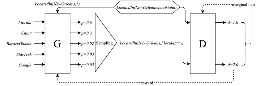
Figure 1: An overview of the kbgan framework. The generator (G) calculates a probability distribution over a set of candidate negative triples, then sample one triples from the distribution as the output. The discriminator (D) receives the generated negative triple as well as the ground truth triple (in the hexagonal box), and calculates their scores. G minimizes the score of the generated negative triple by policy gradient, and D minimizes the marginal loss between positive and negative triples by gradient descent.

Log-softmax loss function is commonly used by models whose score function has probabilistic interpretation. Some notable examples are rescal, DistMult, ComplEx. Applying the softmax function on scores of a given set of triples gives the probability of a triple to be the best one among them: $p(h,r,t)=\frac{\exp f(h,r,t)}{\sum_{(h^{\prime},r,t^{\prime})}\exp f(h^{\prime},r,t^{\prime})}$. The loss function is the negative log-likelihood of this probabilistic model:

$$L_{l}=\sum_{(h,r,t)\in\mathcal{T}}-\log\frac{\exp f(h,r,t)}{\sum\exp f(h^{\prime},r,t^{\prime})}\\ (h^{\prime},r,t^{\prime})\in\{(h,r,t)\}\cup Neg(h,r,t)$$ (2)

where $Neg(h,r,t)\subset\{(h^{\prime},r,t)|h^{\prime}\in\mathcal{E}\}\cup\{(h,r,t^{\prime})|t^{\prime}\in\mathcal{E}\}$ is a set of sampled corrupted triples.

Other forms of loss functions exist, for example ConvE uses a triple-wise logistic function to model how likely the triple is true, but by far the two described above are the most common. Also, softmax function gives an probabilistic distribution over a set of triples, which is necessary for a generator to sample from them.

3.2 Weakness of Uniform Negative Sampling

Most previous KGE models use uniform negative sampling for generating negative triples, that is, replacing the head or tail entity of a positive triple with any of the entities in $\mathcal{E}$, all with equal probability. Most of the negative triples generated in this way contribute little to learning an effective embedding, because they are too obviously false.

To demonstrate this issue, let us consider the following example. Suppose we have a ground truth triple LocatedIn(NewOrleans,Louisiana), and corrupt it by replacing its tail entity. First, we remove the tail entity, leaving LocatedIn(NewOrleans,?). Because the relation LocatedIn constraints types of its entities, “?” must be a geographical region. If we fill “?” with a random entity $e\in\mathcal{E}$, the probability of $e$ having a wrong type is very high, resulting in ridiculous triples like LocatedIn(NewOrleans,BarackObama) or LocatedIn(NewOrleans,StarTrek). Such triples are considered “too easy”, because they can be eliminated solely by types. In contrast, LocatedIn(NewOrleans,Florida) is a very useful negative triple, because it satisfies type constraints, but it cannot be proved wrong without detailed knowledge of American geography. If a KGE model is fed with mostly “too easy” negative examples, it would probably only learn to represent types, not the underlying semantics.

The problem is less severe to models using log-softmax loss function, because they typically samples tens or hundreds of negative triples for one positive triple in each iteration, and it is likely to have a few useful negatives among them. For instance, Trouillon et al. (2016) found that a 100:1 negative-to-positive ratio results in the best performance for ComplEx. However, for marginal loss function, whose negative-to-positive ratio is always 1:1, the low quality of uniformly sampled negatives can seriously damage their performance.

Data: training set of positive fact triples $\mathcal{T}=\{(h,r,t)\}$

Input: Pre-trained generator G with parameters $\theta_{G}$ and score function $f_{G}(h,r,t)$, and pre-trained discriminator D with parameters $\theta_{D}$ and score function $f_{D}(h,r,t)$

Output: Adversarially trained discriminator

$b\longleftarrow 0$;

 // baseline for policy gradient

1 repeat

2       Sample a mini-batch of data $\mathcal{T}_{batch}$ from $\mathcal{T}$ ;

       $G_{G}\longleftarrow 0$, $G_{D}\longleftarrow 0$;

       // gradients of parameters of G and D

       $r_{sum}\longleftarrow 0$;

       // for calculating the baseline

3       for $(h,r,t)\in\mathcal{T}_{batch}$ do

4             Uniformly randomly sample $N_{s}$ negative triples $Neg(h,r,t)=\{(h_{i}^{\prime},r,t_{i}^{\prime})\}_{i=1\dots N_{s}}$;

5             Obtain their probability of being generated: $p_{i}=\frac{\exp f_{G}(h_{i}^{\prime},r,t_{i}^{\prime})}{\sum_{j=1}^{N_{s}}\exp f_{G}(h_{j}^{\prime},r,t_{j}^{\prime})}$;

6             Sample one negative triple $(h_{s}^{\prime},r,t_{s}^{\prime})$ from $Neg(h,r,t)$ according to $\{p_{i}\}_{i=1\dots N_{s}}$. Assume its probability to be $p_{s}$;

             $G_{D}\longleftarrow G_{D}+\nabla_{\theta_{D}}[f_{D}(h,r,t)-f_{D}(h_{s}^{\prime},r,t_{s}^{\prime})+\gamma]_{+}$;

             // accumulate gradients for D

             $r\longleftarrow-f_{D}(h_{s}^{\prime},r,t_{s}^{\prime}),r_{sum}\longleftarrow r_{sum}+r$;

             // $r$ is the reward

             $G_{G}\longleftarrow G_{G}+(r-b)\nabla_{\theta_{G}}\log p_{s}$;

             // accumulate gradients for G

7            

8       end for

      $\theta_{G}\longleftarrow\theta_{G}+\eta_{G}G_{G},\theta_{D}\longleftarrow\theta_{D}-\eta_{D}G_{D}$;

       // update parameters

       $b\leftarrow r_{sum}/|\mathcal{T}_{batch}|$;

       // update baseline

9      

10until convergence;

Algorithm 1 The kbgan algorithm

3.3 Generative Adversarial Training for
Knowledge Graph Embedding Models

Inspired by GANs, we propose an adversarial training framework named kbgan which uses a KGE model with softmax probabilities to provide high-quality negative samples for the training of a KGE model whose training objective is marginal loss function. This framework is independent of the score functions of these two models, and therefore possesses some extent of universality. Figure 1 illustrates the overall structure of kbgan.

In parallel to terminologies used in gan literature, we will simply call these two models generator and discriminator respectively in the rest of this paper. We use softmax probabilistic models as the generator because they can adequately model the “sampling from a probability distribution” process of discrete gans, and we aim at improving discriminators based on marginal loss because they can benefit more from high-quality negative samples. Note that a major difference between gan and our work is that, the ultimate goal of our framework is to produce a good discriminator, whereas gans are aimed at training a good generator. In addition, the discriminator here is not a classifier as it would be in most gans.

Intuitively, the discriminator should assign a relatively small distance to a high-quality negative sample. In order to encourage the generator to generate useful negative samples, the objective of the generator is to minimize the distance given by discriminator for its generated triples. And just like the ordinary training process, the objective of the discriminator is to minimize the marginal loss between the positive triple and the generated negative triple. In an adversarial training setting, the generator and the discriminator are alternatively trained towards their respective objectives.

Suppose that the generator produces a probability distribution on negative triples $p_{G}(h^{\prime},r,t^{\prime}|h,r,t)$ given a positive triple $(h,r,t)$, and generates negative triples $(h^{\prime},r,t^{\prime})$ by sampling from this distribution. Let $f_{D}(h,r,t)$ be the score function of the discriminator. The objective of the discriminator can be formulated as minimizing the following marginal loss function:

$$L_{D}=\sum_{(h,r,t)\in\mathcal{T}}[f_{D}(h,r,t)-f_{D}(h^{\prime},r,t^{\prime})+\gamma]_{+}\\ (h^{\prime},r,t^{\prime})\sim p_{G}(h^{\prime},r,t^{\prime}|h,r,t)$$ (3)

The only difference between this loss function and Equation 1 is that it uses negative samples from the generator.

Model	Hyperparameters	Constraints or Regularizations
TransE	$L_{1}$ distance, $k=50,\gamma=3$	$||\mathbf{e}||_{2}\leq 1,||\mathbf{r}||_{2}\leq 1$
TransD	$L_{1}$ distance, $k=50,\gamma=3$	$||\mathbf{e}||_{2}\leq 1,||\mathbf{r}||_{2}\leq 1,||\mathbf{e_{p}}||_{2}\leq 1,||\mathbf{r_{p}}||_{2}\leq 1$
DistMult	$k=50,\lambda=1/0.1$	L2 regularization: $L_{reg}=L+\lambda||\Theta||_{2}^{2}$
ComplEx	$2k=50,\lambda=1/0.1$	L2 regularization: $L_{reg}=L+\lambda||\Theta||_{2}^{2}$

Table 2: Hyperparameter settings of the 4 models we used. For DistMult and ComplEx, $\lambda=1$ is used for FB15k-237 and $\lambda=0.1$ is used for WN18 and WN18RR. All other hyperparameters are shared among all datasets. $L$ is the global loss defined in Equation (2). $\Theta$ represents all parameters in the model.

Dataset	#r	#ent.	#train	#val	#test
FB15k-237	237	14,541	272,115	17,535	20,466
WN18	18	40,943	141,442	5,000	5,000
WN18RR	11	40,943	86,835	3,034	3,134

Table 3: Statistics of datasets we used in the experiments. “r”: relations.

The objective of the generator can be formulated as maximizing the following expectation of negative distances:

$$R_{G}=\sum_{(h,r,t)\in\mathcal{T}}\mathbb{E}[-f_{D}(h^{\prime},r,t^{\prime})]\\ (h^{\prime},r,t^{\prime})\sim p_{G}(h^{\prime},r,t^{\prime}|h,r,t)$$ (4)

$R_{G}$ involves a discrete sampling step, so we cannot find its gradient with simple differentiation. We use a simple special case of Policy Gradient Theorem Sutton et al. (2000) to obtain the gradient of $R_{G}$ with respect to parameters of the generator:

$$\nabla_{G}R_{G}=\sum_{(h,r,t)\in\mathcal{T}}\mathbb{E}_{(h^{\prime},r,t^{\prime})\sim p_{G}(h^{\prime},r,t^{\prime}|h,r,t)}\\ [-f_{D}(h^{\prime},r,t^{\prime})\nabla_{G}\log p_{G}(h^{\prime},r,t^{\prime}|h,r,t)]\\ \simeq\sum_{(h,r,t)\in\mathcal{T}}\frac{1}{N}\sum_{(h_{i}^{\prime},r,t_{i}^{\prime})\sim p_{G}(h^{\prime},r,t^{\prime}|h,r,t),i=1\dots N}\\ [-f_{D}(h^{\prime},r,t^{\prime})\nabla_{G}\log p_{G}(h^{\prime},r,t^{\prime}|h,r,t)]$$ (5)

where the second approximate equality means we approximate the expectation with sampling in practice. Now we can calculate the gradient of $R_{G}$ and optimize it with gradient-based algorithms.

Policy Gradient Theorem arises from reinforcement learning (RL), so we would like to draw an analogy between our model and an RL model. The generator can be viewed as an agent which interacts with the environment by performing actions and improves itself by maximizing the reward returned from the environment in response of its actions. Correspondingly, the discriminator can be viewed as the environment. Using RL terminologies, $(h,r,t)$ is the state (which determines what actions the actor can take), $p_{G}(h^{\prime},r,t^{\prime}|h,r,t)$ is the policy (how the actor choose actions), $(h^{\prime},r,t^{\prime})$ is the action, and $-f_{D}(h^{\prime},r,t^{\prime})$ is the reward. The method of optimizing $R_{G}$ described above is called reinforce Williams (1992) algorithm in RL. Our model is a simple special case of RL, called one-step RL. In a typical RL setting, each action performed by the agent will change its state, and the agent will perform a series of actions (called an epoch) until it reaches certain states or the number of actions reaches a certain limit. However, in the analogy above, actions does not affect the state, and after each action we restart with another unrelated state, so each epoch consists of only one action.

To reduce the variance of reinforce algorithm, it is common to subtract a baseline from the reward, which is an arbitrary number that only depends on the state, without affecting the expectation of gradients. In our case, we replace $-f_{D}(h^{\prime},r,t^{\prime})$ with $-f_{D}(h^{\prime},r,t^{\prime})-b(h,r,t)$ in the equation above to introduce the baseline. To avoid introducing new parameters, we simply let $b$ be a constant, the average reward of the whole training set: $b=\sum_{(h,r,t)\in\mathcal{T}}\mathbb{E}_{(h^{\prime},r,t^{\prime})\sim p_{G}(h^{\prime},r,t^{\prime}|h,r,t)}[-f_{D}(h^{\prime},r,t^{\prime})]$. In practice, $b$ is approximated by the mean of rewards of recently generated negative triples.

Let the generator’s score function to be $f_{G}(h,r,t)$, given a set of candidate negative triples $Neg(h,r,t)\subset\{(h^{\prime},r,t)|h^{\prime}\in\mathcal{E}\}\cup\{(h,r,t^{\prime})|t^{\prime}\in\mathcal{E}\}$, the probability distribution $p_{G}$ is modeled as:

$$p_{G}(h^{\prime},r,t^{\prime}|h,r,t)=\frac{\exp f_{G}(h^{\prime},r,t^{\prime})}{\sum\exp f_{G}(h^{*},r,t^{*})}\\ (h^{*},r,t^{*})\in Neg(h,r,t)$$ (6)

Ideally, $Neg(h,r,t)$ should contain all possible negatives. However, knowledge graphs are usually highly incomplete, so the ”hardest” negative triples are very likely to be false negatives (true facts). To address this issue, we instead generate $Neg(h,r,t)$ by uniformly sampling of $N_{s}$ entities (a small number compared to the number of all possible negatives) from $\mathcal{E}$ to replace $h$ or $t$. Because in real-world knowledge graphs, true negatives are usually far more than false negatives, such set would be unlikely to contain any false negative, and the negative selected by the generator would likely be a true negative. Using a small $Neg(h,r,t)$ can also significantly reduce computational complexity.

Besides, we adopt the “bern” sampling technique Wang et al. (2014) which replaces the “1” side in “1-to-N” and “N-to-1” relations with higher probability to further reduce false negatives.

Algorithm 1 summarizes the whole adversarial training process. Both the generator and the discriminator require pre-training, which is the same as conventionally training a single KBE model with uniform negative sampling. Formally speaking, one can pre-train the generator by minimizing the loss function defined in Equation (1), and pre-train the discriminator by minimizing the loss function defined in Equation (2). Line 14 in the algorithm assumes that we are using the vanilla gradient descent as the optimization method, but obviously one can substitute it with any gradient-based optimization algorithm.

	FB15k-237		WN18		WN18RR
Method	MRR	H@10	MRR	H@10	MRR	H@10
TransE	-	42.8†	-	89.2	-	43.2†
TransD	-	45.3†	-	92.2	-	42.8†
DistMult	24.1‡	41.9‡	82.2	93.6	42.5‡	49.1‡
ComplEx	24.0‡	41.9‡	94.1	94.7	44.4‡	50.7‡
TransE (pre-trained)	24.2	42.2	43.3	91.5	18.6	45.9
kbgan (TransE + DistMult)	27.4	45.0	71.0	94.9	21.3	48.1
kbgan (TransE + ComplEx)	27.8	45.3	70.5	94.9	21.0	47.9
TransD (pre-trained)	24.5	42.7	49.4	92.8	19.2	46.5
kbgan (TransD + DistMult)	27.8	45.8	77.2	94.8	21.4	47.2
kbgan (TransD + ComplEx)	27.7	45.8	77.9	94.8	21.5	46.9

Table 4: Experimental results. Results of kbgan are results of its discriminator (on the left of the “+” sign). Underlined results are the best ones among our implementations. Results marked with ${\dagger}$ are produced by running Fast-TransX Lin et al. (2015) with its default parameters. Results marked with ${\ddagger}$ are copied from Dettmers et al. (2017). All other baseline results are copied from their original papers.

4 Experiments

To evaluate our proposed framework, we test its performance for the link prediction task with different generators and discriminators. For the generator, we choose two classical probability-based KGE model, DistMult and ComplEx, and for the discriminator, we also choose two classical translation-based KGE model, TransE and TransD, resulting in four possible combinations of generator and discriminator in total. See Table 1 for a brief summary of these models.

4.1 Experimental Settings

4.1.1 Datasets

We use three common knowledge base completion datasets for our experiment: FB15k-237, WN18 and WN18RR. FB15k-237 is a subset of FB15k introduced by Toutanova and Chen (2015), which removed redundant relations in FB15k and greatly reduced the number of relations. Likewise, WN18RR is a subset of WN18 introduced by Dettmers et al. (2017) which removes reversing relations and dramatically increases the difficulty of reasoning. Both FB15k and WN18 are first introduced by Bordes et al. (2013) and have been commonly used in knowledge graph researches. Statistics of datasets we used are shown in Table 3.

4.1.2 Evaluation Protocols

Following previous works like Yang et al. (2015) and Trouillon et al. (2016), for each run, we report two common metrics, mean reciprocal ranking (MRR) and hits at 10 (H@10). We only report scores under the filtered setting Bordes et al. (2013), which removes all triples appeared in training, validating, and testing sets from candidate triples before obtaining the rank of the ground truth triple.

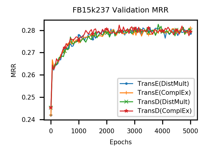
(a)

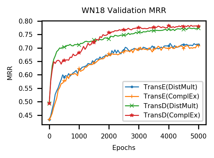
(b)

(c)

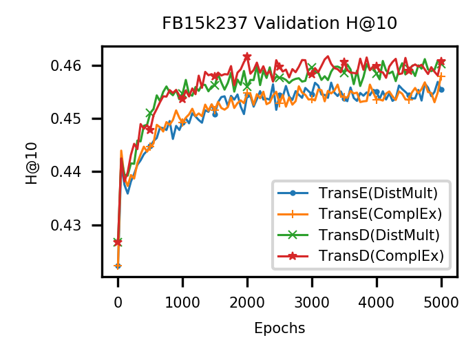
(d)

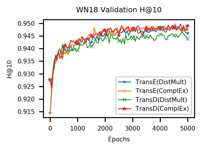
(e)

(f)

Figure 2: Learning curves of kbgan. All metrics improve steadily as training proceeds.

4.1.3 Implementation Details

In the pre-training stage, we train every model to convergence for 1000 epochs, and divide every epoch into 100 mini-batches. To avoid overfitting, we adopt early stopping by evaluating MRR on the validation set every 50 epochs. We tried $\gamma=0.5,1,2,3,4,5$ and $L_{1},L_{2}$ distances for TransE and TransD, and $\lambda=0.01,0.1,1,10$ for DistMult and ComplEx, and determined the best hyperparameters listed on table 2, based on their performances on the validation set after pre-training. Due to limited computation resources, we deliberately limit the dimensions of embeddings to $k=50$, similar to the one used in earlier works, to save time. We also apply certain constraints or regularizations to these models, which are mostly the same as those described in their original publications, and also listed on table 2.

In the adversarial training stage, we keep all the hyperparamters determined in the pre-training stage unchanged. The number of candidate negative triples, $N_{s}$, is set to 20 in all cases, which is proven to be optimal among the candidate set of $\{5,10,20,30,50\}$. We train for 5000 epochs, with 100 mini-batches for each epoch. We also use early stopping in adversarial training by evaluating MRR on the validation set every 100 epochs.

We use the self-adaptive optimization method Adam Kingma and Ba (2015) for all trainings, and always use the recommended default setting $\alpha=0.001,\beta_{1}=0.9,\beta_{2}=0.999,\epsilon=10^{-8}$.

4.2 Results

Results of our experiments as well as baselines are shown in Table 4. All settings of adversarial training bring a pronounced improvement to the model, which indicates that our method is consistently effective in various cases. TransE performs slightly worse than TransD on FB15k-237 and WN18, but better on WN18RR. Using DistMult or ComplEx as the generator does not affect performance greatly.

TransE and TransD enhanced by kbgan can significantly beat their corresponding baseline implementations, and outperform stronger baselines in some cases. As a prototypical and proof-of-principle experiment, we have never expected state-of-the-art results. Being simple models proposed several years ago, TransE and TransD has their limitations in expressiveness that are unlikely to be fully compensated by better training technique. In future researches, people may try employing more advanced models into kbgan, and we believe it has the potential to become state-of-the-art.

To illustrate our training progress, we plot performances of the discriminator on validation set over epochs, which are displayed in Figure 2. As all these graphs show, our performances are always in increasing trends, converging to its maximum as training proceeds, which indicates that kbgan is a robust gan that can converge to good results in various settings, although gans are well-known for difficulty in convergence. Fluctuations in these graphs may seem more prominent than other KGE models, but is considered normal for an adversially trained model. Note that in some cases the curve still tends to rise after 5000 epochs. We do not have sufficient computation resource to train for more epochs, but we believe that they will also eventually converge.

Positive fact	Uniform random sample	Trained generator
(condensation_NN_2, derivationally_related_form, distill_VB_4)	family_arcidae_NN_1 repast_NN_1 beater_NN_2 coverall_NN_1 cash_advance_NN_1	revivification_NN_1 mouthpiece_NN_3 liquid_body_substance_NN_1 stiffen_VB_2 hot_up_VB_1
(colorado_river_NN_2, instance_hypernym, river_NN_1)	lunar_calendar_NN_1 umbellularia_californica_NN_1 tonality_NN_1 creepy-crawly_NN_1 moor_VB_3	idaho_NN_1 sayan_mountains_NN_1 lower_saxony_NN_1 order_ciconiiformes_NN_1 jab_NN_3
(meeting_NN_2, hypernym, social_gathering_NN_1)	cellular_JJ_1 commercial_activity_NN_1 giant_cane_NN_1 streptomyces_NN_1 tranquillize_VB_1	attach_VB_1 bond_NN_6 heavy_spar_NN_1 satellite_NN_1 peep_VB_3

Table 5: Examples of negative samples in WN18 dataset. The first column is the positive fact, and the term in bold is the one to be replaced by an entity in the next two columns. The second column consists of random entities drawn from the whole dataset. The third column contains negative samples generated by the generator in the last 5 epochs of training. Entities in italic are considered to have semantic relation to the positive one

4.3 Case study

To demonstrate that our approach does generate better negative samples, we list some examples of them in Table 5, using the kbgan (TransE + DistMult) model and the WN18 dataset. All hyperparameters are the same as those described in Section 4.1.3.

Compared to uniform random negatives which are almost always totally unrelated, the generator generates more semantically related negative samples, which is different from type relatedness we used as example in Section 3.2, but also helps training. In the first example, two of the five terms are physically related to the process of distilling liquids. In the second example, three of the five entities are geographical objects. In the third example, two of the five entities express the concept of “gather”.

Because we deliberately limited the strength of generated negatives by using a small $N_{s}$ as described in Section 3.3, the semantic relation is pretty weak, and there are still many unrelated entities. However, empirical results (when selecting the optimal $N_{s}$) shows that such situation is more beneficial for training the discriminator than generating even stronger negatives.

5 Conclusions

We propose a novel adversarial learning method for improving a wide range of knowledge graph embedding models—We designed a generator-discriminator framework with dual KGE components. Unlike random uniform sampling, the generator model generates higher quality negative examples, which allow the discriminator model to learn better. To enable backpropagation of error, we introduced a one-step reinforce method to seamlessly integrate the two modules. Experimentally, we tested the proposed ideas with four commonly used KGE models on three datasets, and the results showed that the adversarial learning framework brought consistent improvements to various KGE models under different settings.

References

- Arjovsky et al. (2017) Martin Arjovsky, Soumith Chintala, and Leon Bottou. 2017. Wasserstein gan. In International Conferrence on Machine Learning.
- Bollacker et al. (2008) Kurt Bollacker, Colin Evans, Praveen Paritosh, Tim Sturge, and Jamie Taylor. 2008. Freebase: a collaboratively created graph database for structuring human knowledge. In Proceedings of the 2008 ACM SIGMOD international conference on Management of data. ACM, pages 1247–1250.
- Bordes et al. (2013) Antoine Bordes, Nicolas Usunier, Alberto Garcia-Duran, Jason Weston, and Oksana Yakhnenko. 2013. Translating embeddings for modeling multi-relational data. In Advances in Neural Information Processing Systems. pages 2787–2795.
- Dettmers et al. (2017) Tim Dettmers, Pasquale Minervini, Pontus Stenetorp, and Sebastian Riedel. 2017. Convolutional 2d knowledge graph embeddings. arXiv preprint arXiv:1707.01476 .
- Dong et al. (2014) Xin Dong, Evgeniy Gabrilovich, Geremy Heitz, Wilko Horn, Ni Lao, Kevin Murphy, Thomas Strohmann, Shaohua Sun, and Wei Zhang. 2014. Knowledge vault: A web-scale approach to probabilistic knowledge fusion. In Proceedings of the 20th ACM SIGKDD international conference on Knowledge discovery and data mining. ACM, pages 601–610.
- Goodfellow et al. (2014) Ian Goodfellow, Jean Pouget-Abadie, Mehdi Mirza, Bing Xu, David Warde-Farley, Sherjil Ozair, Aaron Courville, and Yoshua Bengio. 2014. Generative adversarial nets. In Advances in Neural Information Processing Systems. pages 2672–2680.
- Ji et al. (2015) Guoliang Ji, Shizhu He, Liheng Xu, Kang Liu, and Jun Zhao. 2015. Knowledge graph embedding via dynamic mapping matrix. In The 53rd Annual Meeting of the Association for Computational Linguistics.
- Juefei-Xu et al. (2017) Felix Juefei-Xu, Vishnu Naresh Boddeti, and Marios Savvides. 2017. Gang of gans: Generative adversarial networks with maximum margin ranking. arXiv preprint arXiv:1704.04865 .
- Kingma and Ba (2015) Diederik P. Kingma and Jimmy Lei Ba. 2015. Adam: A method for stochastic optimization. In The 3rd International Conference on Learning Representations.
- Krompaß et al. (2015) Denis Krompaß, Stephan Baier, and Volker Tresp. 2015. Type-constrained representation learning in knowledge graphs. In International Semantic Web Conference. Springer, pages 640–655.
- Lin et al. (2015) Yankai Lin, Zhiyuan Liu, Maosong Sun, Yang Liu, and Xuan Zhu. 2015. Learning entity and relation embeddings for knowledge graph completion. In The Twenty-ninth AAAI Conference on Artificial Intelligence. pages 2181–2187.
- Mirza and Osindero (2014) Mehdi Mirza and Simon Osindero. 2014. Conditional generative adversarial nets. arXiv preprint arXiv:1411.01784 .
- Mitchell et al. (2015) Tom M Mitchell, William Cohen, Estevam Hruschka, Partha Talukdar, Justin Betteridge, Andrew Carlson, Bhavana Dalvi Mishra, Matthew Gardner, Bryan Kisiel, Jayant Krishnamurthy, et al. 2015. Never-ending learning. In The Twenty-ninth AAAI Conference on Artificial Intelligence.
- Nickel et al. (2015) Maximilian Nickel, Kevin Murphy, Volker Tresp, and Evgeniy Gabrilovich. 2015. A review of relational machine learning for knowledge graphs. arXiv preprint arXiv:1503.00759 .
- Nickel et al. (2016) Maximilian Nickel, Lorenzo Rosasco, and Tomaso Poggio Poggio. 2016. Holographic embeddings of knowledge graphs. In The Thirtieth AAAI Conference on Artificial Intelligence. pages 1955–1961.
- Nickel et al. (2011) Maximilian Nickel, Volker Tresp, and Hans-Peter Kriegel. 2011. A three-way model for collective learning on multi-relational data. In Proceedings of the 28th International Conference on Machine Learning. pages 809–816.
- Suchanek et al. (2007) Fabian M Suchanek, Gjergji Kasneci, and Gerhard Weikum. 2007. Yago: a core of semantic knowledge. In Proceedings of the 16th international conference on World Wide Web. ACM, pages 697–706.
- Sutton et al. (2000) Richard S Sutton, David A McAllester, Satinder P Singh, and Yishay Mansour. 2000. Policy gradient methods for reinforcement learning with function approximation. In Advances in neural information processing systems. pages 1057–1063.
- Toutanova and Chen (2015) Kristina Toutanova and Danqi Chen. 2015. Observed versus latent features for knowledge base and text inference. In Proceedings of the 3rd Workshop on Continuous Vector Space Models and their Compositionality. pages 57–66.
- Trouillon et al. (2016) Théo Trouillon, Johannes Welbl, Sebastian Riedel, Éric Gaussier, and Guillaume Bouchard. 2016. Complex embeddings for simple link prediction. In International Conference on Machine Learning. pages 2071–2080.
- Wang et al. (2017) Jun Wang, Lantao Yu, Weinan Zhang, Yu Gong, Yinghui Xu, Benyou Wang, Peng Zhang, and Dell Zhang. 2017. Irgan: A minimax game for unifying generative and discriminative information retrieval models. In The 40th International ACM SIGIR Conference.
- Wang et al. (2014) Zhen Wang, Jianwen Zhang, Jianlin Feng, and Zheng Chen. 2014. Knowledge graph embedding by translating on hyperplanes. In The Twenty-eighth AAAI Conference on Artificial Intelligence. pages 1112–1119.
- Williams (1992) Ronald J Williams. 1992. Simple statistical gradient-following algorithms for connectionist reinforcement learning. Machine learning 8(3-4):229–256.
- Xiao et al. (2016) Han Xiao, Minlie Huang, and Xiaoyan Zhu. 2016. From one point to a manifold: Knowledge graph embedding for precise link prediction. In The Twenty-Fifth International Joint Conference on Artificial Intelligence.
- Yang et al. (2015) Bishan Yang, Wen-tau Yih, Xiaodong He, Jianfeng Gao, and Li Deng. 2015. Embedding entities and relations for learning and inference in knowledge bases. The 3rd International Conference on Learning Representations .
- Yu et al. (2017) Lantao Yu, Weinan Zhang, Jun Wang, and Yong Yu. 2017. Seqgan: Sequence generative adversarial nets with policy gradient. In The Thirty-First AAAI Conference on Artificial Intelligence. pages 2852–2858.