Logarithmic superdiffusion in two dimensional driven lattice gases

Abstract

The spreading of density fluctuations in two-dimensional driven diffusive systems is marginally anomalous. Mode coupling theory predicts that the diffusivity in the direction of the drive diverges with time as $(\ln t)^{2/3}$ with a prefactor depending on the macroscopic current-density relation and the diffusion tensor of the fluctuating hydrodynamic field equation. Here we present the first numerical verification of this behavior for a particular version of the two-dimensional asymmetric exclusion process. Particles jump strictly asymmetrically along one of the lattice directions and symmetrically along the other, and an anisotropy parameter $p$ governs the ratio between the two rates. Using a novel massively parallel coupling algorithm that strongly reduces the fluctuations in the numerical estimate of the two-point correlation function, we are able to accurately determine the exponent of the logarithmic correction. In addition, the variation of the prefactor with $p$ provides a stringent test of mode coupling theory.

1 Introduction

Low-dimensional systems with one or several conserved fields often display anomalous dynamics, in the sense that fluctuations spread faster than diffusively. A prominent example is the phenomenon of long-time tails in classical fluids at thermal equilibrium Pomeau1975 ; Forster1977 ; Spohn1991 . In $d$ dimensions the velocity autocorrelation function decays as $t^{-d/2}$ to leading order, which implies diverging transport coefficients in dimensions $d\leq 2$. Specifically, in $d=1$ hydrodynamic modes are governed by the superdiffusive dynamic exponent $z=3/2<2$ vanBeijeren2012 ; Popkov2016 ; Spohn2016 , whereas in the marginal case $d=2$ the corrections to normal diffusion are only logarithmic. Mode coupling theory predicts that the diffusivity diverges as $(\ln t)^{1/2}$ in two dimensions, a behavior that has been notoriously difficult to verify numerically vanderHoef1991 ; Lowe1995 ; Isobe2008

In 1985, van Beijeren, Kutner and Spohn (BKS) discovered a similar scenario for driven diffusive systems (DDS) characterized by a single conserved density onto which a steady current is imposed by an external drive Beij85 . In one dimension such systems are governed by the noisy Burgers equation, which had been studied earlier by Forster, Nelson and Stephen in the hydrodynamic context Forster1977 and was subsequently introduced by Kardar, Parisi and Zhang (KPZ) as a description of stochastic interface dynamics KPZ1986 . The anomalous dynamic exponent $z=3/2$ is now recognized to be the hallmark of the one-dimensional KPZ universality class, and the recent progress in the understanding of one-dimensional fluids relies crucially on previous developments pertaining to the KPZ equation and its various representatives Corwin2012 ; KriKru2010 .

However, in dimensions $d\geq 2$ the DDS and Burgers/KPZ problems are fundamentally different, because the Burgers equation describes the isotropic evolution of a vector field (the height gradient of the KPZ interface) whereas the DDS evolution equation is scalar and anisotropic due to the drive. As a consequence, the strong coupling behavior that characterizes the KPZ equation in dimensions $d\geq 2$ is absent in the DDS case Janssen1986 . Similar to classical fluids, driven diffusive systems display normal diffusive behavior in $d>2$ and are marginally superdiffusive in $d=2$.

Based on mode coupling theory, BKS predicted that the variance of the two-point correlation function in two dimensions grows as $t(\ln t)^{\zeta}$ with $\zeta=2/3$. A rigorous proof of this asymptotics was presented by Yau for the asymmetric simple exclusion process (ASEP) at density $\rho=1/2$ Landim2004 ; Yau04 . On physical grounds one expects the same behavior to apply throughout the class of two-dimensional DDS, but extending the result of Yau to a more general setting has so far remained elusive. In recent work the existence of logarithmic superdiffusivity has been established for a fairly broad class of models, but only upper and lower bounds $1/2\leq\zeta\leq 1$ were obtained for the exponent of the logarithmic correction Quastel2013 .

In this situation it is of interest to explore to what extent logarithmic superdiffusion in two-dimensional DDS can be ascertained using numerical simulations, and, in particular, whether accurate estimates of the exponent $\zeta$ can be obtained. Here we report on large-scale, high-precision simulations of the two-dimensional ASEP that achieve this goal by making use of a novel algorithm based on coupling simulation runs starting from different initial configurations. We believe that our methodology could be useful also in other systems that display marginal superdiffusion, such as two-dimensional hydrodynamic lattice gas models Landim2005 and one-dimensional DDS at densities corresponding to an inflection point of the current-density relation Devillard1992 ; Binder1994 . In both of these cases the exponent $\zeta$ is predicted to take the value $\zeta=1/2$.

In the next section we will define the model used in our study, explain the algorithm and recall the mode coupling theory of BKS. The simulation results are presented in Sect. 3 and some conclusions and consequences for future work are discussed in Sec. 4.

2 Model and methods

2.1 Two-dimensional asymmetric simple exclusion process

Simulations were carried out on a two-dimensional lattice of rectangular shape and with periodic boundary conditions. The lattice is populated with a single species subject to the exclusion principle. For convenience, the overall density was chosen to be $\rho=\frac{1}{2}$, which ensures that the density fluctuations have no systematic drift. As a consequence the two-point correlation function is symmetric and has a stationary peak. The time evolution is computed following a Markov chain Monte Carlo algorithm of random sequential updates. The stochastic dynamics of the system proceeds as follows. At first, the initial state is drawn from the equidistribution on the full configuration space. This amounts to populating the sites of the lattice according to a product measure, with no correlations apart from finite size corrections, which moreover corresponds to the invariant distribution of the dynamics. In a single random sequential update, one independently selects a lattice site from equidistribution and also a direction of motion.

In our implementation of the two-dimensional ASEP particles move strictly asymmetrically along one lattice direction, referred to as the TASEP direction $x_{T}$ in the following, and symmetrically along the perpendicular SSEP direction $x_{S}$. Here TASEP and SSEP stand for the totally asymmetric simple exclusion process and the symmetric simple exclusion process, respectively. Correspondingly, the dimensions of the rectangular lattice $\Gamma={\mathbb{Z}}/L_{\mathrm{T}}\times{\mathbb{Z}}/L_{\mathrm{S}}$ are denoted by $L_{\mathrm{T}}$ and $L_{\mathrm{S}}$. The parameter $p\in(0,1)$ is the probability for choosing the TASEP direction, and $(1-p)/2$ is the probability for the two directions along the SSEP axis. If the target lattice site is empty, the particle moves, otherwise the exclusion principle prohibits the motion and the particle remains on site. Time is counted in units of full system sweeps, where one sweep consists of as many random sequential updates as there are lattice sites. For $p=\frac{1}{2}$ this update rule is the finite size equivalent to the system studied in Yau04 . Below we will make systematic use of the control parameter $p$ for extracting the superdiffusive behavior and for a detailed comparison with the predictions of mode coupling theory.

2.2 Coupling estimator

The quantity of interest is the normalized two-point correlation function

$$S({{\vec{x}}},{{t}})=\kappa^{-1}\left(\left\langle{{n_{{\vec{x}}}({{t}})n_{{\vec{0}}}({{0}})}}\right\rangle-\rho^{2}\right),$$ (1)

where $\left\langle{{\cdot}}\right\rangle$ is the expectation value, $n_{{\vec{x}}}({{t}})\in\{0,1\}$ is the occupation number at site $\vec{x}=(x_{\mathrm{T}},x_{\mathrm{S}})^{T}$ at time $t$, and $\kappa=\rho(1-\rho)$ denotes the compressibility. In standard simulation approaches this two-point correlator is estimated by averaging over all lattice sites (exploiting translation invariance), time evolution (exploiting ergodicity), and many independent realizations (initial states and time evolutions). However, for $S({{\vec{x}}},{{t}})$ these methods fail to reach statistical error bars less than $10^{-6}$ at reasonable computational cost. We estimate an upper bound for numerically accessible system times $t_{\max}$ by requiring data for our analysis with a maximal relative error of 10%. The correlation function can be approximated by a 2D SSEP process whose maximum is analytically known and decays $\propto t^{-1}$. From this, we deduce that the maximally observable time is $t_{\max}\approx 5000$. On the other hand, logarithmic corrections of the kind that we are concerned with here generally require longer times to become visible in the data.

This calls for new ideas to estimate the two-point correlator with significantly lower variance. It turns out that, in this particular case of a single species system, coupling multiple computational runs offers huge advantages. Coupling is a well-established tool in the mathematical analysis of interacting particle systems Liggett1985 ; Liggett1999 , but so far it does not seem to have been exploited much for computational studies (see however Schmidt2015 for a related example). Consider a set of independent initializations $\{n^{({{k}})}_{{\vec{x}}}({{t=0}})\}_{k\in I}$ indexed by $I$ that are coupled in the sense that for their time evolution, in any random sequential update, the same lattice sites and the same directions of motion are drawn in every system. In this way one random number evolves many systems simultaneously and the law of motion can be expressed in bitwise AND and OR operators. This allows one to simulate the coupled systems at no additional cost for a number $|I|$ up to the bitwidth of the computational architecture, which is here always equal to 64.

The defining property of attractive interacting particle systems such as the ASEP is that the configurations of coupled systems approach each other over time Liggett1985 ; Liggett1999 . It is helpful to visualize this process by representing the discrepancies between two configurations by second class particles. For two systems $k,j\in I$, we say there is a discrepancy at site $\vec{x}$ and time $t$ when $n^{({{k}})}_{{\vec{x}}}({{t}})-n^{({{j}})}_{{\vec{x}}}({{t}})=\pm 1$, where the two possible signs define two species of second class particles. Through the dynamics of the coupled systems, second class particles cannot be generated. They are subject to exclusion with first class particles defined by the condition $n^{({{k}})}_{{\vec{x}}}({{t}})=n^{({{j}})}_{{\vec{x}}}({{t}})=1$ and with second class particles of the same sign, and annihilate pairwise whenever a +1 particle meets a $-$1 particle. Thus the number of discrepancies decreases over time and approaches zero for $t\to\infty$. In Fig. 1(a) we show the time evolution of two coupled configurations illustrating this process, and Fig. 1(b) depicts the power law decay of the overall second class particle density

$$\rho^{\mathrm{2nd~{}cl.}}\left({t}\right)\equiv\left\langle{{\frac{1}{\left|{{\Gamma}}\right|}\sum_{\vec{x}\in\Gamma}\left|{{n^{({{k}})}_{{\vec{x}}}({{t}})-n^{({{j}})}_{{\vec{x}}}({{t}})}}\right|}}\right\rangle\stackrel{{\scriptstyle t~{}\text{large}}}{{\simeq}}Ct^{-\beta},\beta=0.56_{\pm 0.01}.$$ (2)

We are not aware of any analytic prediction for the observed exponent $\beta$.

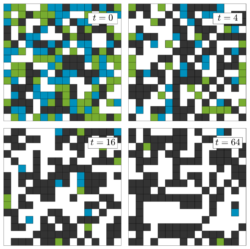
(a)

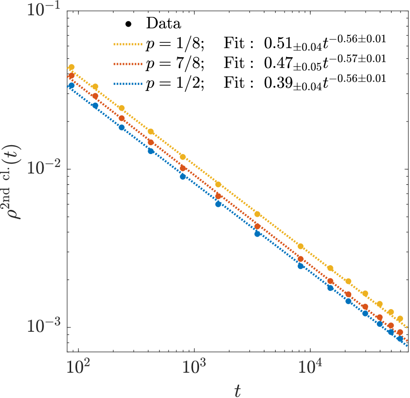
(b)

Figure 1: (a) Exemplary evolution of two coupled $16\times 16$ systems at different times $t$ showing the decay of second-class (colored) particles. Green and blue squares indicate that $n^{({{1}})}_{{\vec{x}}}({{t}})-n^{({{2}})}_{{\vec{x}}}({{t}})=\pm 1$. As the overall particle number in both systems is equal and conserved, the two types of second class particles are equally abundant. (b) Decay of the global second class particle density on double logarithmic scales. While the decay law (2) seems universal, the prefactor $C$ is not monotonic in $p$ and must have a minimum in $(\frac{1}{8},\frac{7}{8})$. Data errors are within the symbol size, computed from 350 independent simulation runs.

Importantly, introducing the coupled systems allows us to express the two-point correlation function in a different manner as

$$\kappa S({{\vec{x}}},{{t}})= \left\langle{{n^{({{k}})}_{{\vec{x}}}({{t}})n^{({{k}})}_{{\vec{0}}}({{0}})}}\right\rangle-\rho^{2}=\left\langle{{n^{({{k}})}_{{\vec{x}}}({{t}})n^{({{k}})}_{{\vec{0}}}({{0}})}}\right\rangle-\left\langle{{n^{({{j}})}_{{\vec{x}}}({{t}})n^{({{k}})}_{{\vec{0}}}({{0}})}}\right\rangle$$

$$= \left\langle{{\left(n^{({{k}})}_{{\vec{x}}}({{t}})-n^{({{j}})}_{{\vec{x}}}({{t}})\right)n^{({{k}})}_{{\vec{0}}}({{0}})}}\right\rangle=\left\langle{{\left(n^{({{k}})}_{{\vec{0}}}({{t}})-n^{({{j}})}_{{\vec{0}}}({{t}})\right)n^{({{k}})}_{{-\vec{x}}}({{0}})}}\right\rangle,$$ (3)

where we used that $n^{({{k}})}_{{\vec{x}}}({{0}})$ and $n^{({{j}})}_{{\vec{y}}}({{t}})$ are independent for $k\neq j$, and that the system is translational invariant. By construction, because $|n^{({{k}})}_{{\vec{x}}}({{t}})-n^{({{j}})}_{{\vec{x}}}({{t}})|$ is often zero for large times, this expression can be efficiently evaluated in simulation data and has fluctuations declining in time. In addition, the relation (2.2) can be exploited for any pair of coupled systems, giving our estimator for the coupled realizations indexed by $I$ as

$$S^{{I}}({{\vec{x}}},{{t}})= \frac{1}{2}\kappa^{-1}\binom{\left|{{I}}\right|}{2}^{-1}\left|{{\Gamma}}\right|^{-1}\times$$

$$\times\sum_{\begin{subarray}{c}k,j\in I,\\ k<j\end{subarray}}\sum_{\vec{y}\in\Gamma}\left(n^{({{k}})}_{{\vec{y}}}({{t}})-n^{({{j}})}_{{\vec{y}}}({{t}})\right)\left(n^{({{k}})}_{{\vec{y}-\vec{x}}}({{0}})-n^{({{j}})}_{{\vec{y}-\vec{x}}}({{0}})\right).$$ (4)

Because of complicated cross-correlations in this expression, we cannot immediately estimate its variance. Nevertheless, if we have $R$ independent realizations of coupled systems indexed by $\left|{{I_{1}}}\right|=\left|{{I_{2}}}\right|=\dots=\left|{{I_{R}}}\right|$, their estimators $\{S^{{I_{r}}}({{t}},{{\vec{x}}})\}_{r}$ are i.i.d. and we may use the standard mean value and error estimates.

2.3 Mode coupling theory

Mode coupling provides a promising inroad for an analytic study of the two-point correlation function, for which the theoretical groundwork was carried out by BKS Beij85 . Therein, the density fluctuations $u({{\vec{x}}},{{t}})$ are described using fluctuating hydrodynamics and the normalized two-point correlation function is expressed through the fluctuation fields as

$$S({{\vec{x}}},{{t}})=\kappa^{-1}\left\langle{{u({{\vec{x}}},{{t}})u({{\vec{0}}},{{0}})}}\right\rangle.$$ (5)

The starting point is the continuity equation

$$\partial_{t}u({{\vec{x}}},{{t}})=\nabla\cdot\left(\mathrm{D}\cdot\nabla u({{\vec{x}}},{{t}})-{\partial_{\rho}\vec{j}}~{}u({{\vec{x}}},{{t}})-\frac{1}{2}~{}{\partial_{\rho}^{2}\vec{j}}~{}u({{\vec{x}}},{{t}})^{2}+B\xi\left(\vec{x},t\right)\right),$$ (6)

where the current is replaced by the steady state current-density relation $\vec{j}(\rho+u({{\vec{x}}},{{t}}))$ expanded up to second order in the fluctuation. Diffusion and white noise with correlations $\left\langle{{\xi\left(\vec{x},t\right)\xi\left(\vec{y},t^{\prime}\right)}}\right\rangle=\delta\left(\vec{x}-\vec{y}\right)\delta\left(t-t^{\prime}\right)$ are added phenomenologically to account for the randomness in the time evolution. With the continuity equation at hand, the mode coupling formalism translates the evolution of the fluctuation fields into an integrodifferential equation for the two-point correlation function known as the mode coupling equation,

$$\partial_{t}S({{\vec{x}}},{{t}})=-{\partial_{\rho}\vec{j}}\cdot\nabla S({{\vec{x}}},{{t}})+\left(\nabla\cdot\mathrm{D}\cdot\nabla\right)S({{\vec{x}}},{{t}})$$

$$+\intop_{0}^{t}\mathrm{d}s\intop\mathrm{d}y^{\mathrm{d}}S({{\vec{x}-\vec{y}}},{{t-s}})M\left(\vec{y},s\right),$$ (7)

where the memory kernel $M$ accounts for nonlinear interactions and noise. The simplest analytically solvable approximation is the one-loop kernel

$$M\left(\vec{y},s\right)=\frac{\kappa}{2}(\partial_{\rho}^{2}\vec{j}\cdot\nabla)^{2}\left(S({{\vec{y}}},{{s}})\right)^{2}.$$ (8)

Solving the mode coupling equation for $d\geq 3$ predicts nonlinear contributions to be irrelevant and therefore a diffusive decay as $\max_{\vec{x}}S({{\vec{x}}},{{t}})\sim t^{-d/z}$ with the diffusive dynamical exponent $z=2$. In contrast, for $d=1$ nonlinear contributions dominate and the asymptotic behavior becomes superdiffusive matching the exact KPZ dynamical exponent $z=3/2$ but failing to recover the exact scaling function Prahofer2004 . Dimension $d=2$ turns out to be the borderline dimension where the diffusion is logarithmically enhanced in the direction of the nonlinearity specified by the unit vector $\vec{e}_{\vec{j}^{\prime\prime}}=\partial_{\rho}^{2}\vec{j}/|\partial_{\rho}^{2}\vec{j}|$ Beij85 .

As controlling diffusion anisotropy will turn out to be crucial for making the logarithmically enhanced diffusion numerically accessible, we present a detailed solution of the two-dimensional mode coupling equation for an arbitrary diffusion tensor. We first perform a Galilean transformation $\vec{\vec{x}}\mapsto\vec{\vec{x}}-t{\partial_{\rho}\vec{j}}$ to remove the drift term and then transform into Fourier space. Using the convention

$$f(\vec{x})=\frac{1}{\left(2\pi\right)^{\mathrm{d}/2}}\intop\mathrm{d}k^{\mathrm{d}}e^{i\vec{k}\cdot\vec{x}}\hat{f}(\vec{k}),\quad\hat{f}(\vec{k})=\frac{1}{\left(2\pi\right)^{\mathrm{d}/2}}\intop\mathrm{d}x^{\mathrm{d}}e^{-i\vec{k}\cdot\vec{x}}f(\vec{x}).$$ (9)

the mode coupling equation becomes

$$-\partial_{t}\hat{S}({{\vec{k}}},{{t}})-\left(\vec{k}\cdot\mathrm{D}\cdot\vec{k}\right)\hat{S}({{\vec{k}}},{{t}})=\intop_{0}^{t}\mathrm{d}s\hat{S}({{\vec{k}}},{{t-s}})\widehat{M}\left(\vec{k},s\right),$$ (10)

with the memory kernel

$$\widehat{M}\left(\vec{k},s\right)=\frac{\kappa\left(\partial^{2}_{\rho}\vec{j}\right)^{2}}{2}\left(\vec{\mathrm{e}}_{\vec{j}^{\prime\prime}}\cdot\vec{k}\right)^{2}\intop\mathrm{d}q^{\mathrm{d}}\hat{S}({{\vec{q}}},{{s}})\hat{S}({{\vec{k}-\vec{q}}},{{s}}).$$ (11)

Similar to Beij85 we account for the logarithmically enhanced diffusion through the scaling ansatz

$$\hat{S}(\vec{k},t)\simeq\frac{1}{2\pi}\exp\left(-(\vec{k}\cdot\mathrm{D}\cdot\vec{k})t-E\left(\vec{\mathrm{e}}_{\vec{j}^{\prime\prime}}\cdot\vec{k}\right)^{2}t(\ln t)^{\zeta}\right).$$ (12)

To capture the asymptotic behavior we take the limit $\left|{{\vec{k}}}\right|\rightarrow 0$ and assume $t$ to be large in the sense of

$$\ln t\gg\left(\frac{\det(\mathrm{D})}{\left(\vec{\mathrm{e}}_{\vec{j}^{\prime\prime}}\cdot\mathrm{adj}(\mathrm{D})\cdot\vec{\mathrm{e}}_{\vec{j}^{\prime\prime}}\right)E}\right)^{1/\zeta}.$$ (13)

Finally, evaluating the left and right hand sides of Eq. (10) gives

$$\frac{E\left(\vec{\mathrm{e}}_{\vec{j}^{\prime\prime}}\cdot\vec{k}\right)^{2}}{2\pi}\cdot(\ln t)^{\zeta}\overset{!}{=}\frac{\kappa\left(\vec{\mathrm{e}}_{\vec{j}^{\prime\prime}}\cdot\vec{k}\right)^{2}}{32\pi^{2}\left(1-\frac{\zeta}{2}\right)\sqrt{\left(\vec{\mathrm{e}}_{\vec{j}^{\prime\prime}}\cdot\mathrm{adj}(\mathrm{D})\cdot\vec{\mathrm{e}}_{\vec{j}^{\prime\prime}}\right)E}}\cdot(\ln t)^{1-\zeta/2}$$ (14)

from which one deduces

$$\zeta=\frac{2}{3}$$ (15)

and

$$E=\left(\frac{3\kappa\left(\partial^{2}_{\rho}\vec{j}\right)^{2}}{32\pi\sqrt{\vec{\mathrm{e}}_{\vec{j}^{\prime\prime}}\cdot\mathrm{adj}(\mathrm{D})\cdot\vec{\mathrm{e}}_{\vec{j}^{\prime\prime}}}}\right)^{2/3}.$$ (16)

Applying this approximation to the system of interest with anisotropy parameter $p$, we have the current-density relation

$$\vec{j}_{p}(\rho)=p\rho(1-\rho)(1,0)^{T}$$ (17)

and the diffusion matrix $\mathrm{D}_{p}=\text{diag}\left({{D_{\mathrm{T},{p}},D_{\mathrm{S},{p}}}}\right)$. Under the reasonable assumption that the diffusion constants scale linearly with the probability of motion in the respective direction, we expect

$$D_{\mathrm{S},{p}}\equiv\overline{D}_{\mathrm{S}}~{}(1-p)=\frac{1-p}{2},~{}~{}D_{\mathrm{T},{p}}=\overline{D}_{\mathrm{T}}~{}p$$ (18)

with universal constants $\overline{D}_{\mathrm{S}},\overline{D}_{\mathrm{T}}$. As will be verified numerically below, $\overline{D}_{\mathrm{S}}$ coincides with the exact diffusion coefficient $\overline{D}_{\mathrm{S}}=\frac{1}{2}$ of the SSEP. With this, the expression (16) reduces to

$$E_{{p}}=E=\frac{1}{8}\left(\frac{3p^{2}}{\pi\sqrt{1-p}}\right)^{2/3}\equiv\overline{E}~{}p\left(\frac{p}{1-p}\right)^{\frac{1}{3}}$$ (19)

with a universal constant $\overline{E}$. Note that according to the condition of Eq. (13), the superdiffusive correction is most easily accessible when $E$ is large, i.e. for $p\to 1$, whereas for small $p$ significant finite-time corrections are expected.

3 Results

3.1 Simulated systems

Simulation data were obtained from six different settings of the anisotropy parameter $p$ and the lattice dimensions (Table 1). They were chosen consistently such that at $t=60000$ the correlations have not yet spread to the boundaries of the system. For this, we chose $\left|{{\Gamma}}\right|\geq 3\cdot 10^{7}$ and the relation between the lattice periodicities was taken to scale with the corresponding probabilities, i.e., $L_{\mathrm{T}}:L_{\mathrm{S}}\approx p:1-p$. The two-point correlation was recorded on a cross of lattice points through the origin parallel to the axes, whose extension scales with the peak width.

TASEP prob.	$p$	$\frac{1}{2}$	$\frac{1}{4}$	$\frac{3}{4}$	$\frac{1}{8}$	$\frac{7}{8}$	$\frac{31}{32}$
TASEP dim.	$L_{\mathrm{T}}$	$6,144$	$4,096$	$12,288$	$2,048$	$16,384$	$32,768$
SSEP dim.	$L_{\mathrm{S}}$	$6,144$	$12,288$	$4,096$	$16,384$	$2,048$	$1,024$
i.i.d. realizations	$R$	$1,000$	$1,000$	$1,000$	$1,000$	$1,000$	$1,000$

Table 1: Summary of ASEP system parameters used in this work.

3.2 Scaling function

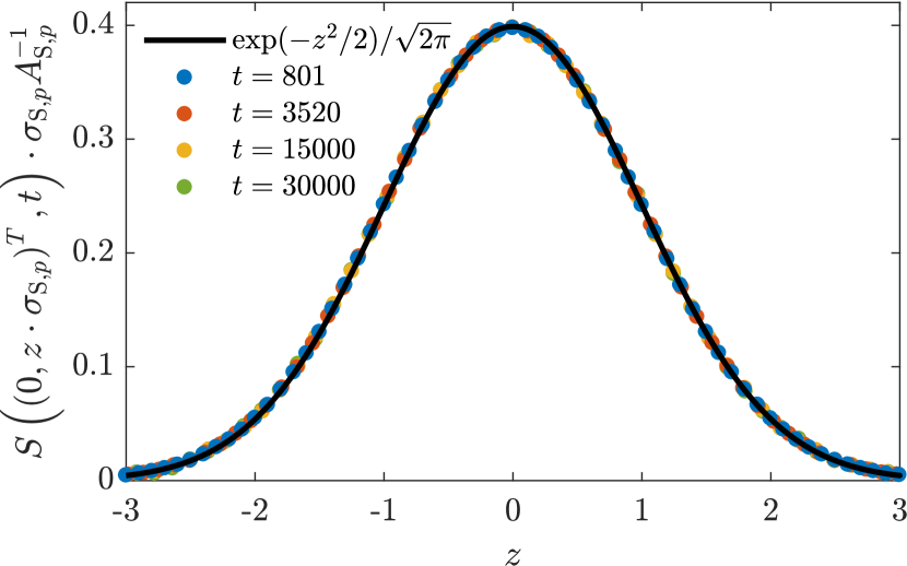
(a)

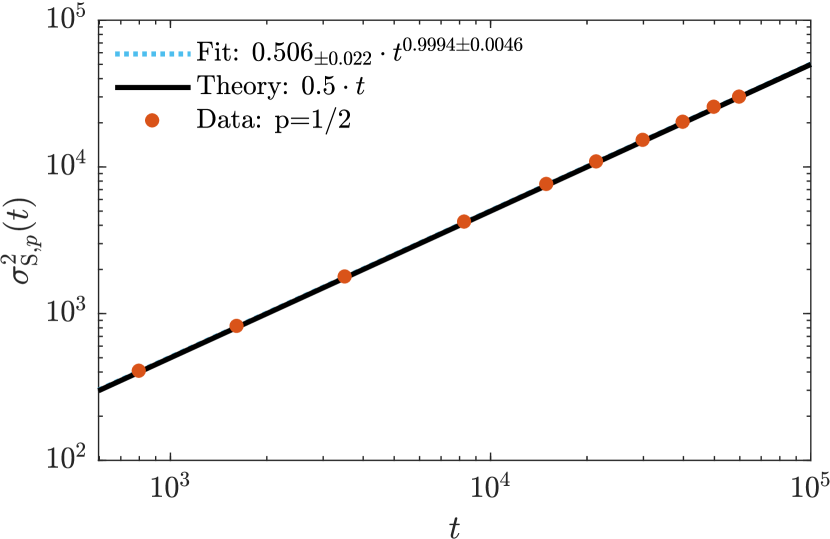
(b)

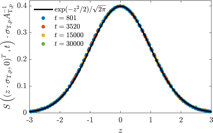
(c)

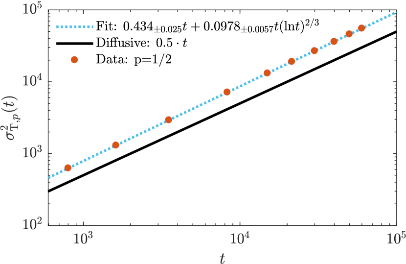
(d)

Figure 2: Scaling function analysis for the $p=\frac{1}{2}$ system. The cross sections along the (a) $x_{\mathrm{S}}$ and (c) $x_{\mathrm{T}}$ directions perfectly collapse to Gaussians. Their variances can be successfully fitted against the theoretical predictions: (b) shows clean diffusion along $x_{\mathrm{S}}$, and (d) indicates the superdiffusive behavior along $x_{\mathrm{T}}$, as the measured variance grows superlinearly. Error bars are within symbol size.

The first object of analysis is the shape of the scaling function. Before analyzing the logarithmic corrections, we want to check that the scaling function indeed factorizes into Gaussians along the two axes. We therefore fit the simulation data to functions of the form

$$S((0,x_{\mathrm{S}})^{T},t)=\frac{A_{\mathrm{S},p}(t)}{\sqrt{2\pi\sigma^{2}_{\mathrm{S},{{p}}}({{t}})}}\exp\left[-\frac{x_{\mathrm{S}}^{2}}{2\sigma^{2}_{\mathrm{S},{{p}}}({{t}})}\right],$$ (20)

$$S((x_{\mathrm{T}},0)^{T},t)=\frac{A_{\mathrm{T},p}(t)}{\sqrt{2\pi\sigma^{2}_{\mathrm{T},{{p}}}({{t}})}}\exp\left[-\frac{x_{\mathrm{T}}^{2}}{2\sigma^{2}_{\mathrm{T},{{p}}}({{t}})}\right].$$ (21)

For the $x_{\mathrm{S}}$ direction, we effectively have coupled symmetric exclusion processes for which it is known that the scaling function is a Gaussian with variance growing $\propto t$. As only a fraction $1-p$ of the moves occur in this direction, we expect $\sigma^{2}_{\mathrm{S},{{p}}}({{t}})=2D_{\mathrm{S},{p}}t=(1-p)t$, which is perfectly verified, see Fig. 2(b). In the fit process, $A_{\mathrm{S},p}(t)$ had to be included as a fit parameter, as it contains the (so far unknown) peak height of the $x_{\mathrm{T}}$-Gaussian. The data in Fig. 2(a) then perfectly collapse on the predicted curve.

For the fit along the $x_{\mathrm{T}}$-axis we make use of the verified prediction $A_{\mathrm{T},p}(t)=(2\pi\sigma^{2}_{\mathrm{S},{{p}}}({{t}}))^{-\frac{1}{2}}=(2\pi(1-p)t)^{-\frac{1}{2}}$ and only fit the peak width. The data again collapse within 99% error bars, see Fig. 2(c). From the variance against time in Fig. 2(d), we can extract the TASEP diffusion constant $D_{\mathrm{T},{p}}$, for which there is no theoretical prediction, and the coefficient $E_{{p}}$ of the superdiffusive logarithmic correction. In the following two subsections we will exploit the $p$-dependence of these quantities in order to extract further information from the simulation data.

3.3 Scaling with the anisotropy parameter $p$

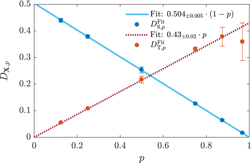
(a)

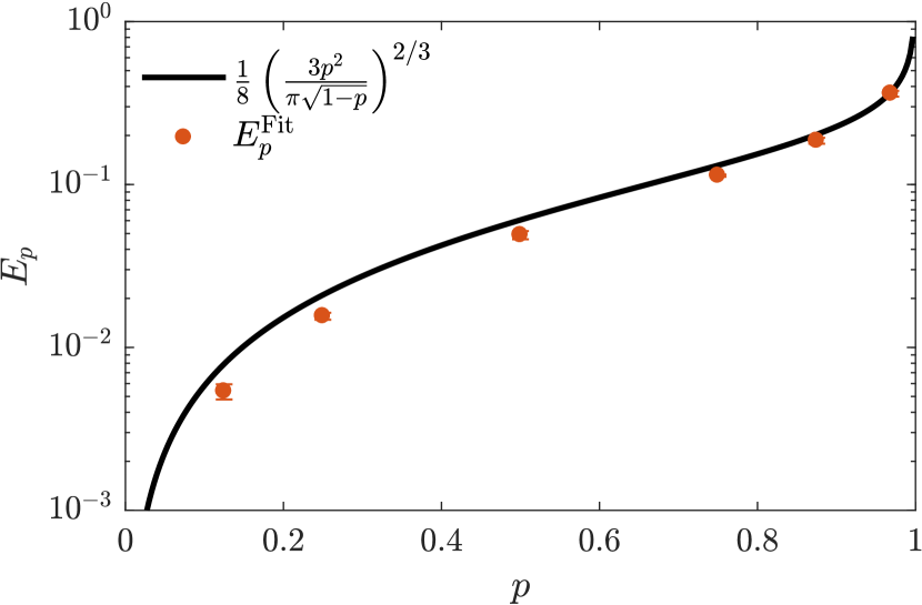
(b)

Figure 3: (a) Diffusion constants $D_{\mathrm{X},p}$ with $X=\mathrm{S}$ or $\mathrm{T}$, and (b) the logarithmic correction coefficient as a function of the anisotropy parameter $p$, fitted from variance data satisfying $\sigma^{2}_{X,p}(t)\gtrsim 400$, resulting in lower bounds $\{3520;~{}1618;~{}801;~{}1618;~{}3520;~{}15000\}$ for $t$. This ensures that the $2\sigma$-regime of the peak spreads on at least 80 lattice sites and the continuum approximation is justified. For the diffusion coefficients the expectation of a linear dependence on $p$ and $1-p$ is well confirmed, but the logarithmic correction coefficient deviates significantly from the theoretical prediction. For the depicted values of $p$, the relative deviation $|E_{p}^{\mathrm{Fit}}-E_{p}|/E_{p}$ takes the values $\{0.32;~{}0.26;~{}0.19;~{}0.45;~{}0.084;~{}0.021\}$.

Using the fit method described in the previous subsection, one can extract the diffusion constants $D_{\mathrm{T},{p}},D_{\mathrm{S},{p}}$ and the coefficient of the logarithmic correction $E_{{p}}$ as a function of $p$. In Fig. 3(a) we verify the linear scaling of the SSEP and TASEP diffusion constants $D_{\mathrm{S},{p}}=\overline{D}_{\mathrm{S}}(1-p),D_{\mathrm{T},{p}}=\overline{D}_{\mathrm{T}}p$ and extract the universal prefactors

$$\overline{D}_{\mathrm{T}}^{\mathrm{Fit}}=0.43\pm 0.02,~{}~{}\overline{D}_{\mathrm{S}}^{\mathrm{Fit}}=0.504\pm 0.005.$$ (22)

As advertised previously, the diffusion constant along the $x_{\mathrm{S}}$ direction agrees with the value $\overline{D}_{\mathrm{S}}=\frac{1}{2}$ expected for the SSEP.

The overall $p$-dependence of the logarithmic correction coefficient $E_{{p}}$ is also well described by the mode coupling prediction (19), but there are significant quantitative deviations particularly for small $p$ (Fig. 3(b)). This should not come as a surprise, since we have seen above in Sect. 2.3 that the convergence to the superdiffusive asymptotics is expected to be fastest for $p$ close to unity. Note, however, that the condition (13) is based on the validity of continuum theory, which requires that the width of the correlation function is large compared to the lattice spacing along both axes. This leads to a loss of accuracy when the one-dimensional limit $p=1$ is approached too closely, as can be seen from the estimate of $D_{\mathrm{T},{p}}$ at $p=\frac{31}{32}$ in Fig. 3(a).

3.4 Logarithmic exponent

So far we have determined the coefficient of the superdiffusive correction assuming that it has the functional form predicted by mode coupling theory. Based on the analyses presented in the preceding subsections, we are now prepared to extract an unbiased estimate for the logarithmic exponent $\zeta$. For this, the crucial idea is to use that the diffusive part of $\sigma^{2}_{\mathrm{T},{{p}}}({{t}})$ scales linearly in $p$, but the logarithmic correction does not. Therefore, for two systems with different anisotropy parameters $p\neq q$, the mode coupling approximation predicts

$$\frac{1}{p}\sigma^{2}_{\mathrm{T},{{p}}}({{t}})-\frac{1}{q}\sigma^{2}_{\mathrm{T},{{q}}}({{t}})= 2\left(\frac{E_{{p}}}{p}-\frac{E_{{q}}}{q}\right)t(\ln t)^{\zeta}$$

$$= 2\overline{E}\left(\left(\frac{p}{1-p}\right)^{\frac{1}{3}}-\left(\frac{q}{1-q}\right)^{\frac{1}{3}}\right)t(\ln t)^{\zeta},$$ (23)

which allows to fit $\zeta$ reliably from the data. As shown in Fig. 4, within error bars this analysis fully confirms the predicted exponent $\zeta=\frac{2}{3}$. By contrast, the prefactor of the logarithmic power law displays some deviations from the prediction of mode coupling theory. However, since these deviations correlate with the errors in the exponent $\zeta$, they might be attributable to finite time corrections.

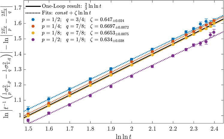
Figure 4: The logarithm of the differences between the rescaled TASEP variances defined in Eq. (3.4) is plotted against doubly logarithmic time. The slopes coincide within error with the theoretical prediction of $\zeta=\frac{2}{3}$. Time $t$ ranges from $88$ to $60000$.

4 Discussion

The work of BKS Beij85 stands at the beginning of a spectacular development that has revealed a universe of interrelated one-dimensional systems, all of which are characterized by the superdiffusive spreading of fluctuations as $t^{2/3}$ Corwin2012 ; KPZ1986 ; KriKru2010 ; GSS2017 . In comparison, the “other $\frac{2}{3}$ -law” discovered by BKS, which is associated with the value of the logarithmic correction exponent $\zeta$ in two-dimensional driven diffusive systems, has received much less attention. Here we have shown that a precise numerical verification of this subtle phenomenon is now possible.

The newly found estimator (2.2) based on the concept of coupling gave us an exciting new tool to push the limits of numerical exploration, such that logarithmic corrections could be made visible. In accordance with the computations of Beij85 , we find strong numerical evidence that (i) the shape of the scaling function is Gaussian, (ii) diffusion is normal along the transverse $x_{\mathrm{S}}$-axis, and (iii) the logarithmic correction term of the variance along the direction $x_{\mathrm{T}}$ of the drive is $\propto t(\ln t)^{\frac{2}{3}}$. The only significant deviations from the theoretical predictions were found in the value of the logarithmic correction coefficient $E$ for small $p$. Since the overall dependence on $p$ is in good agreement with the predictions, these deviations may simply reflect the slow convergence to the asymptotic behavior that is expected for small $p$.

In future work it would be of obvious interest to go beyond the particular version of the ASEP considered here in order to establish the broader universality of the logarithmic superdiffusivity. Whereas certain generalizations of the model can be implemented straightforwardly, others would require further nontrivial innovations in the numerical algorithm. For example, the present method could be easily extended to the case where particles move strictly asymmetrically along the two lattice axes with probability $q$ and $1-q$, respectively, such that the direction of the drive varies continuously with $q$. On the other hand, in the absence of the particle-hole symmetry imposed by the condition $\rho=\frac{1}{2}$, numerical analysis is much harder, because the drift of density fluctuations will strongly increase the systematic errors GSS2017 . In this sense the limitations of the numerical approach are somewhat similar to those encountered in the rigorous analysis of the problem Yau04 , which is also restricted to $\rho=\frac{1}{2}$.

Nevertheless, the idea of using coupling to evolve large ensembles of systems in parallel might offer great opportunities for applications to other problems. In our simple single species model, the coupling between different realizations is complete in the sense that second class particles cannot be generated at all, and our methodology is clearly most efficient for models that share this property. Other applications might be more complex, in that creation of second class particles is allowed. Estimators making use of second class particle extinction due to coupling then still offer a stronger decline in variance until the extinction and creation rate reach equilibrium. More generally, we hope that our work will stimulate further investigations into the dynamics and applications of second class particles, including a theoretical explanation of the power law decay reported in Eq. (2).

Acknowledgments.

We thank Herbert Spohn for his inspiration and leadership, and wish him many years of enjoyable and productive research. This work was supported by Deutsche Forschungsgemeinschaft (DFG) under grant SCHA 636/8-2 and by the University of Cologne through the UoC Forum Classical and quantum dynamics of interacting particle systems.

References

- (1) Y. Pomeau and P. Résibois, Time dependent correlation functions and mode-mode coupling theories. Phys. Rep. 19, 63–139 (1975).
- (2) D. Forster, D.R. Nelson and M.J. Stephen, Large-distance and long-time properties of a randomly stirred fluid. Phys. Rev. A 16, No. 2, 732–749 (1977).
- (3) H. Spohn, Large Scale Dynamics of Interacting Particles (Springer, Heidelberg 1991)
- (4) H. van Beijeren, Exact Results for Anomalous Transport in One-Dimensional Hamiltonian Systems. Phys. Rev. Lett. 108, 180601 (2012).
- (5) V. Popkov, A. Schadschneider, J. Schmidt and G.M. Schütz, Exact scaling solution of the mode coupling equations for non-linear fluctuating hydrodynamics in one dimension. J. Stat. Mech.: Theor. Exp. 093211 (2016).
- (6) H. Spohn, Fluctuating hydrodynamics approach to equilibrium time correlations for anharmonic chains. In “Thermal transport in low dimensions: from statistical physics to nanoscale heat transfer”, ed. S. Lepri. Springer Lecture Notes in Physics, Volume 921, pp. 107–158 (Springer, Heidelberg 2016).
- (7) M.A. van der Hoef and D. Frenkel, Evidence for Faster-than- Decay of the Velocity Autocorrelation Function in a 2D Fluid. Phys. Rev. Lett. 66, 1591–1594 (1991).
- (8) C.P. Lowe and D. Frenkel, The super long-time decay of velocity fluctuations in a two-dimensional fluid. Physica A 220, 251–260 (1995).
- (9) M. Isobe, Long-time tail of the velocity autocorrelation function in a two-dimensional moderately dense hard-disk fluid. Phys. Rev. E 77, 021201 (2008).
- (10) H. van Beijeren, R. Kutner, and H. Spohn, Excess noise for driven diffusive systems. Phys. Rev. Lett. 54, no. 18, 2026–2029 (1985).
- (11) M. Kardar, G. Parisi and Y-C. Zhang, Dynamic scaling of growing interfaces. Phys. Rev. Lett. 56, 889–892 (1986).
- (12) I. Corwin, The Kardar-Parisi-Zhang equation and universality class. Random Matrices: Theory Appl. 1, 1130001 (2012).
- (13) T. Kriecherbauer and J. Krug, A pedestrian’s view on interacting particle systems, KPZ universality and random matrices. J. Phys. A 43, 403001 (2010).
- (14) H.K. Janssen and B. Schmittmann, Field Theory of Long Time Behaviour in Driven Diffusive Systems. Z. Phys. B 63, 517–520 (1986).
- (15) C. Landim, J. Quastel, M. Salmhofer and H.-T. Yau, Superdiffusivity of Asymmetric Exclusion Process in Dimensions One and Two. Commun. Math. Phys. 244, 455–481 (2004).
- (16) H.-T. Yau, -law of the two dimensional asymmetric simple exclusion process. Ann. of Math. (2) 159, no. 1, 377–405 (2004).
- (17) J. Quastel and B. Valkó, Diffusivity of Lattice Gases. Arch. Rational Mech. Anal. 210, 269–320 (2013).
- (18) C. Landim, J.A. Ramirez and H.-T. Yau, Superdiffusivity of Two Dimensional Lattice Gas Models. J. Stat. Phys. 119, Nos. 5/6, 963–995 (2005).
- (19) P. Devillard and H. Spohn, Universality Class of Interface Growth with Reflection Symmetry. J. Stat. Phys. 66, Nos. 3/4, 1089–1099 (1992).
- (20) P.-M. Binder, M. Paczuski and M. Barma, Scaling of fluctuations in one-dimensional interface and hopping models. Phys. Rev. E 49, no. 2, 1174–1181 (1994).
- (21) T.M. Liggett, Interacting Particle Systems (Springer, New York 1985).
- (22) T.M. Liggett, Stochastic Interacting Particle Systems: Contact, Voter and Exclusion Processes (Springer, New York 1999).
- (23) J. Schmidt, V. Popkov and A. Schadschneider, Defect-induced phase transition in the asymmetric simple exclusion process. EPL 110, 20008 (2015).
- (24) M. Prähofer and H. Spohn, Exact scaling function for one-dimensional stationary KPZ growth. J. Stat. Phys. 115, 255–279 (2004).
- (25) J. de Gier, A. Schadschneider and J. Schmidt, KPZ universality of the Nagel-Schreckenberg Model. in preparation