Abstract

A model for neutrino masses and mixing is presented using the see-saw mechanism. The model combines Type -I and Type-II see-saw contributions of which the latter dominates. The scalars and the leptons in the model are assigned $A4$ charges suitable to obtain the mass matrices required for the scheme. The Type -II see-saw accommodates atmospheric mass splitting and maximal mixing in the atmospheric sector ($\theta_{23}=\pi/4$). It is characterized by vanishing solar mass splitting and $\theta_{13}$ whereas the third neutrino mixing angle can acquire any value, $\theta_{12}^{0}$. Particular alternatives of $\theta_{12}^{0}$ viz. $\theta_{12}^{0}=35.3^{\circ}$ (tribimaximal), $45.0^{\circ}$ (bimaximal), $31.7^{\circ}$ (golden ratio) are accounted for. Another choice of $\theta_{12}^{0}=0^{\circ}$ (no solar mixing) is also considered. Incorporating the corrections provided by the subdominant Type-I see-saw involves degenerate perturbation theory due to vanishing solar splitting in the Type -II see-saw enabling the solar mixing angle to receive substantial corrections. Apart from amending the solar sector the Type-I see-saw also tunes all the neutrino oscillation parameters into the allowed ranges thus interrelating them all. Thus the model is testable in the light of future experimental data. As an example, $\theta_{23}$ emerges in the first (second) octant for normal (inverted) ordering. CP-violation is controlled by phases present in the right-handed Majorana neutrino mass matrix, $M_{\nu R}$. Only normal ordering is allowed if these phases are absent. If $M_{\nu R}$ is complex the Dirac CP-violating phase $\delta$, can be large, i.e., $\sim\pm\pi/2$, and inverted ordering is also allowed. T2K and NOVA preliminary data favouring normal ordering and $\delta\sim-\pi/2$ predicts lightest neutrino mass to be 0.05 eV or more within the model framework.

PACS No:  14.60.Pq
Key Words:  Neutrino mixing, $\theta_{13}$, Solar splitting, A4, see-saw, Leptonic CP-violation

I Introduction

Intensive experimental investigations worldwide have determined neutrino masses and mixing to a great extent. In spite of these neutrinos retain certain mysteries including the ordering of their masses, their absolute mass scale, their Dirac or Majorana nature, the octant of the atmospheric mixing angle $\theta_{23}$ and CP-violation in lepton sector. While future experiments address these riddles, here a model of neutrino masses and mixing in concord with the experimental observations is proposed. The two small quantities $\theta_{13}$ and the ratio, $R\equiv\Delta m^{2}_{solar}/\Delta m^{2}_{atmos}$ can get interrelated when both are derived from a single perturbation [1]. In [2] larger mixing parameters like $\Delta m^{2}_{atmos}$ and $\theta_{23}=\pi/4$ were ascribed to the dominant fundamental structure of neutrino masses and mixing whereas the other oscillation parameters i.e., $\theta_{13},\theta_{12}$, the deviation of $\theta_{23}$ from $\pi/4$, and $\Delta m^{2}_{solar}$ originated from a smaller see-saw [3] generated perturbation. This induces constraints on the measured parameters. Certain symmetries can give rise to vanishing $\theta_{13}$ rather easily and new models based on perturbations of such structures are also common in literature [5, 6]. Here, a schematic outline of the current exercise is given. The following standard parametrization of the lepton mixing matrix – the Pontecorvo, Maki, Nakagawa, Sakata (PMNS) matrix – $U$ has been used

$$U=\left(\begin{array}[]{ccc}c_{12}c_{13}&s_{12}c_{13}&s_{13}e^{-i\delta}\\ -c_{23}s_{12}+s_{23}s_{13}c_{12}e^{i\delta}&c_{23}c_{12}+s_{23}s_{13}s_{12}e^{i\delta}&s_{23}c_{13}\\ s_{23}s_{12}+c_{23}s_{13}c_{12}e^{i\delta}&-s_{23}c_{12}+c_{23}s_{13}s_{12}e^{i\delta}&c_{23}c_{13}\end{array}\right)\;\;,$$ (4)

where $c_{ij}=\cos\theta_{ij}$ and $s_{ij}=\sin\theta_{ij}$. Neutrino masses and mixing are generated by a two-component Lagrangian, one of the dominant Type-II see-saw kind while the subdominant contribution originates from Type-I see-saw. The larger atmospheric mass splitting, $\Delta m^{2}_{atmos}$ and maximal atomspheric mixing ($\theta_{23}=\pi/4$) is embedded within the Type-II see-saw structure whereas the solar splitting, $\Delta m^{2}_{solar}$ and $\theta_{13}$ are kept to be zero. The solar mixing angle can vary continuously and acquire any desired value of $\theta_{12}^{0}$. Needless to mention that neither $\Delta m^{2}_{solar}$ nor $\theta_{13}$ are vanishing [7]. Evidences of non-maximal yet large $\theta_{23}$ exist. The solar mixing angle $\theta_{12}$ is also constrained by experiments. The Type-I see-saw alleviates all these issues. Since the solar splitting is vanishing in the Type-II see-saw scenario, the first two mass eigenstates are degenerate. In order to lift this degeneracy with the help of Type-I see-saw contribution one has to use degenerate perturbation theory. As a consequence of this, corrections to the solar mixing angle can be large. The starting structure can be of tribimaximal (TBM), bimaximal (BM), and golden ratio (GR) mixings. All of these have $\theta_{13}=0$ and $\theta_{23}=\pi/4$, $\theta_{12}^{0}$ being the only discriminating factor as specified in Table 1. In this Table, the fourth option corresponds to no solar mixing (NSM) i.e., $\theta_{12}^{0}=0$ which has the virtue of the mixing angles to be either maximal, i.e., $\pi/4$ ($\theta_{23}$) or vanishing ($\theta_{13}$ and $\theta_{12}^{0}$). An $A4$-based model with identical objectives only for the NSM case was studied in [8]. This attempt along with [8] differ from the other earlier works on $A4$ [9, 10, 11] as in most of them neutrino mass matrix was derived as an outcome of a Type-II see-saw mechanism and obtaining TBM was of chief importance. Recent activities directed towards more realistic mixing patterns [12] often leading to breaking of $A4$ symmetry can be found in [13]. A few distinctive aspects of this model are worth noting at this point. Firstly, a combination of Type-I and Type-II see-saw is considered. Secondly, the model is constructed to accommodate many popular mixing patterns. This is the first attempt of this kind using $A4$ flavour symmetry that amends several popular lepton mixing patterns in a single stroke in which Type-II see-saw is the dominant contribution whereas Type-I see-saw is the subdominant component. The symmetries are broken spontaneously. Further, soft symmetry breaking terms are prohibited. All symmetry conserving terms are included in the Lagrangian. Scalars and leptons involved in the model are assigned suitable $A4$ charges to implement this feature. An analogous pursuit based on $S3\times Z3$ resulted in [14].

Model	TBM	BM	GR	NSM
$\theta^{0}_{12}$	35.3∘	45.0∘	31.7∘	0.0∘

Table 1: $\theta^{0}_{12}$ for different popular lepton mixing patterns viz. TBM, BM, and GR mixing. NSM represents the case with vanishing solar mixing.

All the three neutrino mixing angles and the solar mass splitting receives first order corrections from a single source – the Type -I see-saw in this model. Owing to the common origin, they all get interrelated. These correlations are characteristic features of this particular model. Indeed the model has a large number of parameters, but it must noted that only the region of the parameter space allowed by the neutrino mass and mixing data obeying these correlations is considered. An analysis of the model initiates the discussion. In the next section, the operational strategy is described. The results so obtained are compared to the experimental data in the following section, succeeded by the conclusions and inferences of this work. Some essential ideas of the of the discrete symmetry $A4$ are presented in Appendix A. A detailed study of the rich scalar sector to the extent of local minimization of the scalar potential is furnished in Appendix B. In Appendix C algebraic details of the mass matrix calculations while going to the flavour basis of the neutrinos from the Lagrangian basis can be found.

II The Mass Model

The model comprises of scalars and leptons with specific $A4$ charges. All terms allowed by the symmetries under consideration are included in the Lagrangian. No soft symmetry-breaking term is included.

Fields	Notations	$A4$	$SU(2)_{L}$ ($Y$)	$L$
Left-handed leptons	$(\nu_{i},l_{i})_{L}$	3	2 (-1)	1
	$l_{1R}$	1
Right-handed charged leptons	$l_{2R}$	$1^{\prime}$	1 (-2)	1
	$l_{3R}$	$1^{\prime\prime}$
Right-handed neutrinos	$N_{iR}$	3	1 (0)	-1

Table 2: The lepton catalogue of the model. The $A4$ quantum numbers assignments of the fields are featured together with their $SU(2)_{L}$ properties. The hypercharge, $Y$, and lepton number, $L$, are displayed.

The right-handed charged leptons transform as $1(e_{R})$, $1^{\prime}(\mu_{R})$, and $1^{\prime\prime}(\tau_{R})$ under $A4$. The left-handed lepton doublets of three flavours constitute an $A4$ triplet, so does the right-handed neutrinos. Table 2 shows the lepton constituents of the model together with their transformation properties under $A4$ and $SU(2)_{L}$. The hypercharge and lepton number assignments are also shown. The choices of $A4$ properties of the fields are not unique. A list of all possible options can be found in [15] of which this model adopts class B. The model is restricted to leptons only.

Purpose	Notations	$A4$	$SU(2)_{L}$	$L$	$vev$
			($Y$)
Charged fermion mass	$\Phi=\pmatrix{\phi_{1}^{+}&\phi_{1}^{0}\cr\phi_{2}^{+}&\phi_{2}^{0}\cr\phi_{3}^{+}&\phi_{3}^{0}}$	3	2 (1)	0	$\langle\Phi\rangle=\frac{v}{\sqrt{3}}\pmatrix{0&1\cr 0&1\cr 0&1}$
Neutrino Dirac mass	$\eta=(\eta^{0},\eta^{-})$	1	2 (-1)	2	$\langle\eta\rangle=\pmatrix{u,0}$
Type-II see-saw mass	$\hat{\Delta}^{L}_{a}=\pmatrix{\hat{\Delta}^{++}_{1a}&\hat{\Delta}^{+}_{1a}&\hat{\Delta}^{0}_{1a}\cr\hat{\Delta}^{++}_{2a}&\hat{\Delta}^{+}_{2a}&\hat{\Delta}^{0}_{2a}\cr\hat{\Delta}^{++}_{3a}&\hat{\Delta}^{+}_{3a}&\hat{\Delta}^{0}_{3a}}^{L}$	3	3 (2)	-2	$\langle\hat{\Delta}^{L}_{a}\rangle=v_{La}\pmatrix{0&0&1\cr 0&0&0\cr 0&0&0}$
Type-II see-saw mass	$\hat{\Delta}^{L}_{b}=\pmatrix{\hat{\Delta}^{++}_{1b}&\hat{\Delta}^{+}_{1b}&\hat{\Delta}^{0}_{1b}\cr\hat{\Delta}^{++}_{2b}&\hat{\Delta}^{+}_{2b}&\hat{\Delta}^{0}_{2b}\cr\hat{\Delta}^{++}_{3b}&\hat{\Delta}^{+}_{3b}&\hat{\Delta}^{0}_{3b}}^{L}$	3	3 (2)	-2	$\langle\hat{\Delta}^{L}_{b}\rangle=v_{Lb}\pmatrix{0&0&1\cr 0&0&1\cr 0&0&1}$
		1	3 (2)	-2	$\langle\Delta_{1}^{L}\rangle=\pmatrix{0,0,u_{L}}$
Type-II see-saw mass	$\Delta_{\zeta}^{L}=(\Delta_{\zeta}^{++},\Delta_{\zeta}^{+},\Delta_{\zeta}^{0})^{L}$	$1^{\prime}$	3 (2)	-2	$\langle\Delta_{2}^{L}\rangle=\pmatrix{0,0,u_{L}}$
		$1^{\prime\prime}$	3 (2)	-2	$\langle\Delta_{3}^{L}\rangle=\pmatrix{0,0,u_{L}}$
Right-handed neutrino mass	$\hat{\Delta}^{R}_{a}=\pmatrix{\hat{\Delta}^{0}_{1a}\cr\hat{\Delta}^{0}_{2a}\cr\hat{\Delta}^{0}_{3a}}^{R}$	3	1 (0)	2	$\langle\hat{\Delta}^{R}_{a}\rangle=v_{Ra}\pmatrix{1\cr 1\cr 1}$
Right-handed neutrino mass	$\hat{\Delta}^{R}_{b}=\pmatrix{\hat{\Delta}^{0}_{1b}\cr\hat{\Delta}^{0}_{2b}\cr\hat{\Delta}^{0}_{3b}}^{R}$	3	1 (0)	2	$\langle\hat{\Delta}^{R}_{b}\rangle=v_{Rb}\pmatrix{1\cr\omega\cr\omega^{2}}$
Right-handed neutrino mass	$\hat{\Delta}^{R}_{c}=\pmatrix{\hat{\Delta}^{0}_{1c}\cr\hat{\Delta}^{0}_{2c}\cr\hat{\Delta}^{0}_{3c}}^{R}$	3	1 (0)	2	$\langle\hat{\Delta}^{R}_{c}\rangle=v_{Rc}\pmatrix{1\cr\omega^{2}\cr\omega}$
Right-handed neutrino mass	$\Delta_{1}^{R}=(\Delta_{1}^{0})^{R}$	$1$	1 (0)	2	$\langle\Delta_{1}^{R}\rangle={u}_{1R}$
Right-handed neutrino mass	$\Delta_{2}^{R}=(\Delta_{2}^{0})^{R}$	$1^{\prime}$	1 (0)	2	$\langle\Delta_{2}^{R}\rangle={u}_{2R}$
Right-handed neutrino mass	$\Delta_{3}^{R}=(\Delta_{3}^{0})^{R}$	$1^{\prime\prime}$	1 (0)	2	$\langle\Delta_{3}^{R}\rangle={u}_{3R}$

Table 3: The scalar sector of the model. The $A4$ charges as well as the $SU(2)_{L}$ nature of the scalars are exhibited. The hypercharge ,$Y$, lepton number, $L$, and the vacuum expectation value (vev) configurations of the scalars are also presented.

Masses of all leptons originate from $A4$-invariant Yukawa couplings. Several scalar fields have to be included that acquire suitable vacuum expectation values (vevs). The strategy of choosing the scalar field multiplets requires some elaboration. An idea of the mass matrices of the left- and right-handed neutrinos in the flavour basis (charged lepton mass matrix diagonal) that are suitable for our avowed goal can be acquired from our previous work [14]. The Lagrangian is written down in a basis which is unitarily related to the flavour basis. Consequently, the mass matrices in this defining basis have somewhat complicated structures for which the motivation is not initially obvious. These forms of the mass matrices (below) arise from a rather large set of scalars and their vevs.

The charged leptons acquire their masses through the $SU(2)_{L}$ doublet scalar fields $\Phi_{i}~{}(i=1,2,3)$ forming an $A4$ triplet. The neutrino Dirac mass matrix is generated by an $A4$ invariant $SU(2)_{L}$ doublet $\eta$, having lepton number 2. $SU(2)_{L}$ triplet scalars are required for the Type-II see-saw for left-handed neutrino mass matrix that include $A4$ triplet fields $\hat{\Delta}_{a}^{L}$ and $\hat{\Delta}_{b}^{L}$ along with $\Delta_{\zeta}^{L},~{}\zeta=1,2,3$ transforming as $1$, $1^{\prime}$, $1^{\prime\prime}$ of $A4$. These are used to construct the dominant Type-II see-saw neutrino mass matrix. Effects of the subdominant Type-I see-saw contribution is included perturbatively. $A4$ conserving Yukawa couplings produce the right-handed neutrino mass matrix as well. Several $SU(2)_{L}$ singlet scalars are involved in generation of the Majorana masses for the right-handed neutrinos viz. $\hat{\Delta}^{R}_{p}$ ($p=a,b,c$) transforming as $A4$ triplets and $\Delta^{R}_{\gamma}$ ($\gamma=1,2,3$) transforming as $1$, $1^{\prime}$ and $1^{\prime\prime}$ under $A4$. Table 3 evinces transformation properties of the model scalars under $A4$ and $SU(2)_{L}$ together with their hypercharge, lepton number and vev configurations. The vevs of the $SU(2)_{L}$ doublet scalars are of ${\cal O}(M_{W})$ while that of the $SU(2)_{L}$ triplets are several orders of magnitude smaller than the doublet vevs in concord with the small neutrino masses as well as the $\rho$ parameter of electroweak symmetry breaking. As expected, the vevs of the $SU(2)_{L}$ singlets responsible for right-handed neutrino mass lies much above the electroweak scale. The mass terms of the neutrinos (both Type-I and Type-II see-saw) and that of the charged leptons are generated by a $SU(2)_{L}\times U(1)_{Y}$ conserving Lagrangian that preserves $A4$ as well:

$$\mathscr{L}_{mass} = y_{j}\rho_{jik}\bar{l}_{Li}l_{Rj}\Phi_{k}^{0}~{}~{}{\rm(charged~{}lepton~{}mass)}$$ (5)

$$+ f\rho_{1ik}\bar{\nu}_{Li}N_{Rk}\eta^{0}~{}~{}{\rm(neutrino~{}Dirac~{}mass)}$$

$$+ \frac{1}{2}\left(\sum_{n=a,b}\hat{Y}^{L}_{n}~{}\alpha_{ijk}\nu_{Li}^{T}C^{-1}\nu_{Lj}\hat{\Delta}_{nk}^{L0}+Y^{L}_{\zeta}~{}\rho_{\zeta ij}\nu_{Li}^{T}C^{-1}\nu_{Lj}\Delta_{\zeta}^{L0}\right)~{}~{}{\rm(neutrino~{}Type\!-\!II~{}see\!-\!saw~{}mass)}$$

$$+ \frac{1}{2}\left(\sum_{p=a,b,c}\hat{Y}^{R}_{p}~{}\alpha_{ijk}N_{Ri}^{T}C^{-1}N_{Rj}\hat{\Delta}_{kp}^{R0}+Y^{R}_{\gamma}~{}\rho_{\gamma ij}N_{Ri}^{T}C^{-1}N_{Rj}\Delta_{\gamma}^{R0}\right)~{}~{}{\rm(rh~{}neutrino~{}mass)}+h.c.$$

The scalars acquire the following vevs ($SU(2)_{L}$ part is suppressed):

$$\langle\Phi^{0}\rangle=\frac{v}{\sqrt{3}}\pmatrix{1\cr 1\cr 1}\;,\;\langle\eta^{0}\rangle=u\;,\langle\hat{\Delta}^{L0}_{a}\rangle=v_{La}\pmatrix{1\cr 0\cr 0}\;,\;\langle\hat{\Delta}^{L0}_{b}\rangle=v_{Lb}\pmatrix{1\cr 1\cr 1}\;,\;\langle\Delta_{1}^{L0}\rangle=\langle\Delta_{2}^{L0}\rangle=\langle\Delta_{3}^{L0}\rangle={u}_{L}\;,$$ (6)

$$\langle\hat{\Delta}^{R0}_{a}\rangle=v_{Ra}\pmatrix{1\cr 1\cr 1}\;,\;\langle\hat{\Delta}^{R0}_{b}\rangle=v_{Rb}\pmatrix{1\cr\omega\cr\omega^{2}}\;,\;\langle\hat{\Delta}^{R0}_{c}\rangle=v_{Rc}\pmatrix{1\cr\omega^{2}\cr\omega}\;,\;$$ (7)

$$\langle\Delta_{1}^{R0}\rangle={u}_{1R}\;,\;\langle\Delta_{2}^{R0}\rangle={u}_{2R}\;,\;\langle\Delta_{3}^{R0}\rangle={u}_{3R}\;.\;$$ (8)

An elaborate study of the $A4$ conserving scalar potential involving the fields listed in Table 3 is presented in Appendix B of this paper. Local minimization is performed and the conditions corresponding to the particular vev structures as indicated in Eqs. (6-8) are obtained. The mass matrix for the charged leptons and the left-handed Majorana neutrinos so obtained are:

$$M_{e\mu\tau}=\frac{v}{\sqrt{3}}\pmatrix{y_{1}&y_{2}&y_{3}\cr y_{1}&\omega y_{2}&\omega^{2}y_{3}\cr y_{1}&\omega^{2}y_{2}&\omega y_{3}}\;,\;M_{\nu L}=\pmatrix{(Y^{L}_{1}+2Y^{L}_{2})u_{L}&\frac{1}{2}\hat{Y}^{L}_{b}v_{Lb}&\frac{1}{2}\hat{Y}^{L}_{b}v_{Lb}\cr\frac{1}{2}\hat{Y}^{L}_{b}v_{Lb}&(Y^{L}_{1}-Y^{L}_{2})u_{L}&\frac{1}{2}(\hat{Y}^{L}_{a}v_{La}+\hat{Y}^{L}_{b}v_{Lb})\cr\frac{1}{2}\hat{Y}^{L}_{b}v_{Lb}&\frac{1}{2}(\hat{Y}^{L}_{a}v_{La}+\hat{Y}^{L}_{b}v_{Lb})&(Y^{L}_{1}-Y^{L}_{2})u_{L}},$$ (9)

where the choice of $Y^{L}_{2}=Y^{L}_{3}$ is made. The Yukawa couplings involved in the charged lepton mass matrix satisfies $y_{1}v=m_{e},~{}y_{2}v=m_{\mu},~{}y_{3}v=m_{\tau}$. The neutrino mass matrix of Dirac nature and the right-handed neutrino mass matrix of Majorana kind acquires the following structures:

$$M_{D}=fu~{}\mathbb{I}\;\;,\;\;M_{\nu R}=m_{R}\pmatrix{\chi_{1}&\chi_{6}&\chi_{5}\cr\chi_{6}&\chi_{2}&\chi_{4}\cr\chi_{5}&\chi_{4}&\chi_{3}}\;\;.$$ (10)

$m_{D}$ sets the scale of Dirac masses of the neutrinos where one can identify $fu=m_{D}$. The scale of the Type-II see-saw neutrino masses is much smaller than that of the charged leptons i.e., ${\cal O}(M_{\nu L})\sim u_{L},v_{La},v_{Lb}$ where $u_{L},v_{La},v_{Lb}<<v$. Such a possibility that the triplet vev is much smaller than the doublet vev can be obtained as shown in [18], albeit in a model with fewer scalars. The scale of the right-handed Majorana neutrino masses is set by $m_{R}$ and $\chi_{i}$ in Eq. (10) are dimensionless quantities of ${\cal O}(1)$. The mass matrices in Eq. (9) could be expressed in a more convenient form by applying a couple of transformations. The non-hermitian charged lepton mass matrix can be diagonalised by applying a transformation $U_{L}$ (below) on the left-handed lepton doublets and no transformation on the right-handed charged leptons. The transformation matrices are expressed as:

$$U_{L}={1\over{\sqrt{3}}}\pmatrix{1&1&1\cr 1&\omega^{2}&\omega\cr 1&\omega&\omega^{2}}\;.$$ (11)

This basis in which the charged lepton mass matrix is diagonal and the entire lepton mixing is governed by the neutrino sector is termed as the flavour basis in which the mass matrices acquire the following forms:

$$M_{e\mu\tau}^{flavour}=\pmatrix{m_{e}&0&0\cr 0&m_{\mu}&0\cr 0&0&m_{\tau}}\;\;,\;\;M_{\nu L}^{flavour}={1\over 2}\pmatrix{2m^{(0)}_{1}&0&0\cr 0&m^{+}&m^{-}\cr 0&m^{-}&m^{+}}\;\;.$$ (12)

Here $m^{\pm}\equiv m_{3}^{(0)}\pm m_{1}^{(0)}$. Therefore, $m^{-}$ is positive (negative) for normal (inverted) ordering. As noted earlier, $M_{\nu L}^{flavour}$, which arises from the Type-II see-saw, is the dominant contribution to the neutrino mass. Demanding that the neutrino Dirac mass matrix, which couples the left- and right-handed neutrinos, preserves its proportionality to the identity matrix necessitates that the transformation applied on the right-handed neutrino fields must be $V_{R}=U_{L}$. Thus we get,

$$M_{D}=fu~{}\mathbb{I}\;\;,\;\;M_{\nu R}^{flavour}=(V_{R}^{\dagger}\,M_{\nu R}\,V_{R}^{\dagger})={m_{R}\over 4ab}\pmatrix{r_{11}&r_{12}&r_{13}\cr r_{12}&r_{22}&r_{23}\cr r_{13}&r_{23}&r_{33}}\;\;.$$ (13)

The matrices in Eq. (13) will take part in the Type-I see-saw mechanism. Various identification of the products of the Yukawa couplings and the vevs with the neutrino mass and mixing parameters are necessary for the mass matrices to be expressed in the forms as presented in Eqs. (12) and (13). Appendix C comprises of these algebraic details.

III Modus Operandi

The four mass matrices in the flavour basis obtained from the model are given in Eq. (12) and (13). In this basis the entire lepton mixing and CP-violation is controlled solely by the neutrino sector to which we restrict our discussion now onwards. The Type-II see-saw derived $M_{\nu L}^{flavour}$ is the dominant component to which the subdominant contribution attributed by the Type-I see-saw is incorporated by perturbation theory. The flavour basis mass matrices have to undergo one more basis transformations for successful implementation of this scheme. More precisely they ought to be expressed in the mass basis of the neutrinos which by definition has the left-handed neutrino mass matrix diagonal in it. Thus,

$$M^{0}=M_{\nu L}^{mass}=U^{0T}M_{\nu L}^{flavour}U^{0}=\pmatrix{m^{(0)}_{1}&0&0\cr 0&m^{(0)}_{1}&0\cr 0&0&m^{(0)}_{3}}\;\;,$$ (14)

where,

$$U^{0}=\pmatrix{\cos\theta_{12}^{0}&\sin\theta_{12}^{0}&0\cr-\frac{\sin\theta_{12}^{0}}{\sqrt{2}}&\frac{\cos\theta_{12}^{0}}{\sqrt{2}}&{1\over\sqrt{2}}\cr\frac{\sin\theta_{12}^{0}}{\sqrt{2}}&-\frac{\cos\theta_{12}^{0}}{\sqrt{2}}&{1\over\sqrt{2}}}.$$ (15)

The left-handed neutrino fields in the mass basis ($|\nu_{L}^{mass}\rangle$) are connected to the ones in the flavour basis ($|\nu_{L}^{flavour}\rangle$) by this $U^{0}$ furnished in Eq. (15). One can obtain the $|\nu_{L}^{mass}\rangle$ by applying $U^{0\dagger}$ on $|\nu_{L}^{flavour}\rangle$ i.e., $|\nu_{L}^{mass}\rangle=U^{0\dagger}|\nu_{L}^{flavour}\rangle$. It immediately follows from Eqs. (14), (4) and (15) that in the Type-II see-saw component solar splitting is absent, $\theta_{13}=0$ and $\theta_{23}=\pi/4$. The columns of $U^{0}$ are the unperturbed flavour basis. Once again we demand that in the mass basis the neutrino Dirac mass matrix remains proportional to identity. In order to satisfy this the same transformation ($U^{0\dagger}$) has to be applied on the right-handed neutrino fields. This leads to changes in form of right-handed neutrino mass matrix given by $M_{\nu R}^{mass}=(U^{0\dagger}\,M_{\nu R}^{flavour}\,U^{0})$. The matrices contributing in Type-I see-saw are as follows:

$$M_{D}=m_{D}\mathbb{I}\ \ {\rm and}\ \ M_{\nu R}^{mass}=\frac{m_{R}}{2\sqrt{2}ab}\pmatrix{0&b&b\cr b&\frac{a}{\sqrt{2}}&-\frac{a}{\sqrt{2}}\cr b&-\frac{a}{\sqrt{2}}&\frac{a}{\sqrt{2}}}\ \ .$$ (16)

Here $a$ and $b$ are dimensionless quantities of ${\cal O}(1)$. It is imperative to note that $a$ and $b$ can in general be complex. One can in principle trade off $a$ and $b$ in terms of complex numbers $ye^{-i\phi_{2}}$ and $xe^{-i\phi_{1}}$ respectively, where $x$ and $y$ are dimensionless real quantities of ${\cal O}(1)$. The Type-I see-saw contribution so obtained is given by:

$$M^{\prime}=\left[M_{D}^{T}(M_{\nu R})^{-1}M_{D}\right]={m_{D}^{2}\over m_{R}}\pmatrix{0&y~{}e^{i\phi_{1}}&y~{}e^{i\phi_{1}}\cr y~{}e^{i\phi_{1}}&{x~{}e^{i\phi_{2}}\over\sqrt{2}}&{-x~{}e^{i\phi_{2}}\over\sqrt{2}}\cr y~{}e^{i\phi_{1}}&{-x~{}e^{i\phi_{2}}\over\sqrt{2}}&{x~{}e^{i\phi_{2}}\over\sqrt{2}}}\;\;.$$ (17)

Here the Dirac mass matrix is proportional to identity. It was checked that the same results can follow as long as $M_{D}$ is diagonal. $M_{\nu R}^{mass}$ exhibits a $N_{2R}\leftrightarrow N_{3R}$ discrete symmetry. The results remain intact even if that choice is relaxed. Now onwards the entire procedure is carried on in the mass basis of the neutrinos using the mass matrices expressed in Eqs. (14) and (17). The method followed below essentially consists of the following steps. Form the Type-II see-saw a lepton mixing of the form of Eq. (15) is generated, with $\theta_{12}^{0}$ of any preferred value. At this stage, only the atmospheric mass splitting is non-zero and atmospheric mixing is maximal. Next, the Type-I see-saw is included using degenerate perturbation theory. The solar mass splitting and the desired $\theta_{12}$ are first obtained. Then the third column of the mixing matrix is calculated and compared with Eq. (4) to extract $\theta_{13}$, $\theta_{23}$, and $\delta$.

IV Results

The neutrino mass matrices derived from Type-I and Type-II see-saw mechanism have been discussed in the previous section, of which the former is significantly smaller than the latter. In absence of the Type-I see-saw contribution the leptonic mixing matrix is characterized by $\theta_{13}=0$, $\theta_{23}=\pi/4$, and $\theta_{12}^{0}$ is free to vary. Consequences for four choices of the value of $\theta_{12}^{0}$ corresponding to TBM, BM, GR, and NSM cases together with vanishing solar splitting are examined. This along with the atmospheric mass splitting allowed by the data depict the Type-II see-saw structure. Inclusion of Type-I see-saw corrections perturbatively up to first order modulates the neutrino oscillation parameters into the ranges preferred by data. Owing to the vanishing solar splitting in the Type-II see-saw contribution the first two mass eigenstates are degenerate. Thus in the solar sector degenerate perturbation theory has to be applied. Hence the first order corrections to the solar mixing angle can be large. The global best-fit of the oscillation parameters are displayed in the next section.

IV.1 Data

The current 3$\sigma$ global fits of the neutrino oscillation parameters are: [19, 20]

$$\Delta m_{21}^{2} = (7.02-8.08)\times 10^{-5}\,{\rm eV}^{2},\;\;\theta_{12}=(31.52-36.18)^{\circ},$$

$$|\Delta m_{31}^{2}| = (2.351-2.618)\times 10^{-3}\,{\rm eV}^{2},\;\;\theta_{23}=(38.6-53.1)^{\circ}\,,$$

$$\theta_{13} = (7.86-9.11)^{\circ},\;\;\delta=(0-360)^{\circ}\;\;.$$ (18)

These numbers are taken from NuFIT2.1 of 2016 [19]. Needless to mention, $\Delta m_{ij}^{2}\equiv m_{i}^{2}-m_{j}^{2}$, such that $\Delta m_{31}^{2}>0$ for normal ordering (NO) and $\Delta m_{31}^{2}<0$ for inverted ordering (IO). Two best-fit points of $\theta_{23}$ are evinced by the data in the first and in the second octants. Towards the end of the paper it is discussed how the model can accommodate the recent T2K and NOVA hints [21, 22] of $\delta$ close to -$\pi/2$.

IV.2 Real $M_{\nu R}$ ($\phi_{1}=0~{}{\rm or}~{}\pi,\phi_{2}=0~{}{\rm or}~{}\pi$)

As a warm-up exercise let us consider the simpler case of $M_{\nu R}$ real. In such a scenario there is no CP-violation as the phases $\phi_{1,2}$ of Eq. (17) are 0 or $\pi$. This leads to four different alternatives available for choosing $\phi_{1}$ and $\phi_{2}$. These are captured compactly by taking $x$ and $y$ real and allowing them to assume both signs for notational convenience. It will be soon clear how the experimental observations prefer one or the other of these four alternatives. Thus for real $M_{\nu R}$ the Type -I see-saw contribution appears like:

$$M^{\prime}={m_{D}^{2}\over m_{R}}\pmatrix{0&y&y\cr y&{x\over\sqrt{2}}&-{x\over\sqrt{2}}\cr y&-{x\over\sqrt{2}}&{x\over\sqrt{2}}}\;\;.$$ (19)

The degeneracy of the two neutrino masses in the Type-II see-saw ensuring the vanishing solar splitting necessitates the application of degenerate perturbation theory to obtain the corrections for the solar sector mixing parameters . The entire dynamics of this sector is dictated by the upper $2\times 2$ submatrix of $M^{\prime}$ given by:

$$M^{\prime}_{2\times 2}={m_{D}^{2}\over m_{R}}\pmatrix{0&y\cr y&{x/\sqrt{2}}}\;.$$ (20)

This gives rise to:

$$\theta_{12}=\theta_{12}^{0}+\zeta\;\;,\;\;\tan 2\zeta=2\sqrt{2}\left(\frac{y}{x}\right)\;.$$ (21)

Model ($\theta^{0}_{12}$)	TBM (35.3∘)	BM (45.0∘)	GR (31.7∘)	NSM (0.0∘)
$\zeta$	-4.0${}^{\circ}\leftrightarrow$ 0.6∘	-13.7${}^{\circ}\leftrightarrow$ -9.1∘	-0.4${}^{\circ}\leftrightarrow$ 4.2∘	31.3${}^{\circ}\leftrightarrow$ 35.9∘
$\epsilon$	-4.0${}^{\circ}\leftrightarrow$ 0.6∘	-14.5${}^{\circ}\leftrightarrow$ -9.3∘	-0.4${}^{\circ}\leftrightarrow$ 4.2∘	44.0${}^{\circ}\leftrightarrow$ 56.7∘
$\epsilon-\theta_{12}^{0}$	-39.2${}^{\circ}\leftrightarrow$ -34.6∘	-59.5${}^{\circ}\leftrightarrow$ -54.4∘	-39.2${}^{\circ}\leftrightarrow$ -30.0∘	44.0${}^{\circ}\leftrightarrow$ 56.7∘

Table 4: Data allowed $3\sigma$ ranges of $\zeta$ (Eq. (21)), $\epsilon$ (Eq. (22)), and $(\epsilon-\theta_{12}^{0})$ for different popular mixing patterns are shown.

For functional ease it is useful to define a quantity, $\epsilon$ as:

$$\sin\epsilon=\frac{y}{\sqrt{y^{2}+x^{2}/2}}\;\;{\rm and}~{}\cos\epsilon=\frac{x/\sqrt{2}}{\sqrt{y^{2}+x^{2}/2}}\;\;,\;\;{\rm i.e.,}~{}\tan\epsilon=\frac{1}{2}\tan 2\zeta\;.$$ (22)

Once a mixing pattern is selected, the corresponding $\theta_{12}^{0}$ gets fixed and the experimental bounds of $\theta_{12}$ determines the $3\sigma$ ranges of $\zeta$ and $\epsilon$ by means of Eq. (18) and Eq. (22) as featured in Table 4. The ratio $(y/x)$ is positive (negative) when $\zeta$ is positive (negative). From Eq. (22) it is evident that the sign of $y$ is regulated by the value of $\epsilon$. Putting all these facts together it is easy to infer that $x$ is positive always, or in other words $\phi_{2}$ must be 0, while $y$ has to be positive, $\phi_{1}=0$ (negative, $\phi_{1}=\pi$) for NSM (BM). In case of TBM and GR, both signs of $y$ are admissible. The solar splitting provided by the Type-I see-saw as extracted from Eq. (20) is:

$$\Delta m^{2}_{solar}={\sqrt{2}m_{D}^{2}\over m_{R}}~{}m^{(0)}_{1}\sqrt{x^{2}+8y^{2}}={\sqrt{2}m_{D}^{2}\over m_{R}}~{}m^{(0)}_{1}\frac{x}{\cos 2\zeta}\;\;.$$ (23)

For the mass basis form of the mass matrix in Eq. (14), the mixing in the leptonic sector is completely given by the $U^{0}$ given in Eq. (15). After including the Type-I see-saw correction to the mass matrices there is a further contribution to the mixing matrix as well, now given by:

$$U=U^{0}U_{\nu}\;{\rm where}~{}U_{\nu}=\pmatrix{\cos\zeta&-\sin\zeta&\kappa_{r}\sin\epsilon\cr\sin\zeta&\cos\zeta&-\kappa_{r}\cos\epsilon\cr\kappa_{r}\sin(\zeta-\epsilon)&\kappa_{r}\cos(\zeta-\epsilon)&1}\;,$$ (24)

with

$$\kappa_{r}\equiv{m_{D}^{2}\over{m_{R}m^{-}}}\sqrt{y^{2}+x^{2}/2}={m_{D}^{2}\over{m_{R}m^{-}}}\frac{x}{\sqrt{2}\cos\epsilon}\;\;.$$ (25)

The third column of the lepton mixing matrix is:

$$|\psi_{3}\rangle=\pmatrix{\kappa_{r}\sin(\epsilon-\theta_{12}^{0})\cr{1\over\sqrt{2}}{[1-\kappa_{r}\cos(\epsilon-\theta_{12}^{0})]}\cr{1\over\sqrt{2}}{[1+\kappa_{r}\cos(\epsilon-\theta_{12}^{0})]}}\ \ \ .$$ (26)

As already pointed out, $x$ is always positive, $\kappa_{r}$ is positive (negative) for NO (IO).

Eq. (26) when mapped to the third column of Eq. (4) leads to:

$$\sin\theta_{13}\cos\delta=\kappa_{r}\sin(\epsilon-\theta_{12}^{0})\;\;,$$ (27)

and

$$\tan(\pi/4-\theta_{23})\equiv\tan\omega=\kappa_{r}\cos(\epsilon-\theta_{12}^{0})\;.$$ (28)

The allowed ranges of $(\epsilon-\theta_{12}^{0})$ for the different mixing patterns is given in Table 4 . The CP-phase $\delta$ is 0 ($\pi$) when $\sin(\epsilon-\theta_{12}^{0})$ is positive (negative) in case of normal ordering. It can be immediately concluded that $\delta=0$ for the NSM from Table 4 and $\delta=\pi$ for the rest of the options under study. CP is conserved for both the values of $\delta$.

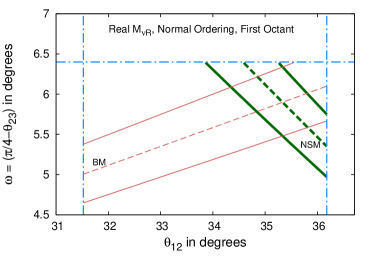
Figure 1: $\omega=(\pi/4-\theta_{23})$ -vs- $\theta_{12}$ plot for normal ordering. The $3\sigma$ allowed range of $\sin\theta_{13}$ is marked by the solid lines whereas the dashed line indicates the best-fit value. Thin pink (thick green) lines denote the BM (NSM) case. The horizontal and vertical lines represent the data allowed 3$\sigma$ range. The first octant of $\theta_{23}$ is preferred since $\omega$ is positive always. Although $\omega$ is positive for TBM and GR mixing patterns its value lies beyond the $3\sigma$ range. Best-fit values of atmospheric and solar mass splittings are taken. Inverted ordering is disallowed for $M_{\nu R}$ real.

Using Eqs. (23), (25), and (27) it can be found:

$$\Delta m^{2}_{solar}=2~{}m^{-}m^{(0)}_{1}~{}\frac{\sin\theta_{13}\cos\delta\cos\epsilon}{\cos 2\zeta~{}\sin(\epsilon-\theta_{12}^{0})}\;\;.$$ (29)

For real $M_{\nu R}$ inverted ordering is forbidden as can be seen from Eq. (29). In order to justify this one can define:

$$z\equiv m^{-}m^{(0)}_{1}/\Delta m^{2}_{atmos}\;\;{\rm and}\;\;\tan\xi\equiv m_{0}/\sqrt{|\Delta m^{2}_{atmos}|}\;\;,$$ (30)

where $z$ is positive for both the orderings of neutrino masses. With the help of Eq. (29) it can be written as:

$$z=\left(\frac{\Delta m^{2}_{solar}}{|\Delta m^{2}_{atmos}|}\right)\left(\frac{\cos 2\zeta~{}\sin(\epsilon-\theta_{12}^{0})}{2\sin\theta_{13}|\cos\delta|\cos\epsilon}\right)\;\;.$$ (31)

From Eq. (30) it is straightforward to show that:

$$z = \sin\xi/(1+\sin\xi)\;\;{\rm~{}i.e.,}\;\;0\leq z\leq\frac{1}{2}\;\;{\rm(for~{}normal~{}ordering)},$$

$$z = 1/(1+\sin\xi)\;\;{\rm~{}i.e.,}\;\;\frac{1}{2}\leq z\leq 1\;\;{\rm(for~{}inverted~{}ordering)}\;\;.$$ (32)

The lightest neutrino mass $m_{0}$ has a one-to-one correspondence with $z$. In the quasi-degenerate limit, i.e., $m_{0}\rightarrow$ large, $z\rightarrow\frac{1}{2}$ for both orderings. For real $M_{\nu R}$, $|\cos\delta|=1$ in Eq. (31). It simply follows from the global fit mass splittings and mixing angles in Sec. IV.1 and Table 4 that $z\sim 10^{-2}$ or smaller for all four popular mixing alternatives. Thus inverted ordering is forbidden for real $M_{\nu R}$.

Using Eqs. (27) and (28) the deviation of the atmospheric mixing angle from maximality is found to be:

$$\tan\omega=\frac{\sin\theta_{13}\cos\delta}{\tan(\epsilon-\theta_{12}^{0})}\;\;.$$ (33)

Eq. (28) implies that $\omega$ is positive always for normal ordering irrespective of the mixing pattern. Thus $\theta_{23}$ is confined only to the first octant for real $M_{\nu R}$. $\epsilon$ can be expressed in terms of $\theta_{12}$ using Eqs. (21) and (22). Thus $\omega$ in Eq. (33) can be expressed as a function of $\theta_{13}$ and $\theta_{12}$ only. Fig. 1 exhibits $\omega$ as a function of $\theta_{12}$ for BM (thin pink lines) and NSM (thick green lines) alternatives. $\theta_{12}$ and $\omega$ varied within 3$\sigma$ allowed ranges as shown in Sec. IV.1. The TBM and GR cases are excluded owing as for the allowed values of $\theta_{12}$ they predict $\theta_{23}$ beyond the 3$\sigma$ range. The 3$\sigma$ limiting values of $\theta_{13}$ are marked by the solid lines whereas the dashed lines indicate its best-fit value. The vertical and horizontal blue dot-dashed lines denote the 3$\sigma$ experimental limits of $\theta_{12}$ and $\theta_{23}$.

With the help of Eq. (31), one can translate any allowed point in the $\omega-\theta_{12}$ plane and the $\theta_{13}$ associated with it to a value of $z$ or equivalently $m_{0}$, when the solar and the atmospheric mass splittings are provided. For both the allowed mixing patterns $m_{0}$ varies over a very small range. This range is found to be $2.13$ meV $\leq m_{0}\leq 3.10$ meV ($3.20$ meV $\leq m_{0}\leq 4.42$ meV) for NSM (BM) when both mass splittings and all the three mixing angles are allowed to vary over their entire 3$\sigma$ ranges.

The salient features of real $M_{\nu R}$ case are:

1. Only the normal ordering of neutrino masses is allowed.

2. Only the first octant of $\theta_{23}$ is admissible.

3. Type-I see-saw corrections is unable to make the TBM and GR mixing patterns consistent with the allowed ranges of the mixing angles.

4. NSM and BM alternatives can produce solutions in agreement with the observed neutrino masses and mixing. The allowed ranges of lightest neutrino mass is very narrow.

IV.3 Complex $M_{\nu R}$

Real $M_{\nu R}$ has several limitations viz. inverted ordering and CP-violation is forbidden. Moreover TBM and GR mixing patterns cannot be included within the ambit of the model when $M_{\nu R}$ is real. In order to overcome these constraints the general complex form of $M_{\nu R}$ leading to Type-I see-saw contribution $M^{\prime}$ furnished in Eq. (17) has to be considered. It is worth reminding ourselves that this choice introduces the complex phases $\phi_{1,2}$ while $x$ and $y$ can only be positive.

Thus, $M^{\prime}$ is no longer hermitian. To retain the hermitian nature the combination $(M^{0}+M^{\prime})^{\dagger}(M^{0}+M^{\prime})$ is considered among which $M^{0\dagger}M^{0}$ and $(M^{0\dagger}M^{\prime}+M^{\prime\dagger}M^{0})$ are treated as the leading term and the perturbation at the lowest order respectively. The unperturbed eigenvalues are given by $(m^{(0)}_{i})^{2}$ and perturbation matrix is:

$$(M^{0\dagger}M^{\prime}+M^{\prime\dagger}M^{0})={m_{D}^{2}\over m_{R}}\pmatrix{0&2ym^{(0)}_{1}\cos\phi_{1}&yf(\phi_{1})\cr 2ym^{(0)}_{1}\cos\phi_{1}&\sqrt{2}xm^{(0)}_{1}\cos\phi_{2}&-{x\over\sqrt{2}}f(\phi_{2})\cr yf^{*}(\phi_{1})&-{x\over\sqrt{2}}f^{*}(\phi_{2})&\sqrt{2}xm^{(0)}_{3}\cos\phi_{2}}\;,$$ (34)

where,

$$f(\varphi)\equiv m^{+}\cos\varphi-im^{-}\sin\varphi\;\;.$$ (35)

The rest of the procedure is analogous to what was done in case of real $M_{\nu R}$ keeping in mind the discriminating factors of Eq. (34). Now, instead of Eqs. (21) and (22) of the real $M_{\nu R}$ case, the solar mixing obtained from Eq. (34) is given by

$$\theta_{12}=\theta_{12}^{0}+\zeta\;\;,\;\;\tan 2\zeta=2\sqrt{2}~{}{y\over x}~{}{\cos\phi_{1}\over\cos\phi_{2}}\;\;,$$ (36)

and

$$\sin\epsilon=\frac{y\cos\phi_{1}}{\sqrt{y^{2}\cos^{2}\phi_{1}+x^{2}\cos^{2}\phi_{2}/2}}\;\;,\;\;\cos\epsilon=\frac{x\cos\phi_{2}/\sqrt{2}}{\sqrt{y^{2}\cos^{2}\phi_{1}+x^{2}\cos^{2}\phi_{2}/2}}\;\;,\;\;\tan\epsilon=\frac{1}{2}\tan 2\zeta\;.$$ (37)

Mixing	Normal Ordering		Inverted Ordering
Pattern	$\delta$	$\theta_{23}$	$\delta$	$\theta_{23}$
	quadrant	octant	quadrant	octant
NSM	First/Fourth	First	Second/Third	Second
BM, TBM, GR	Second/Third	First	First/Fourth	Second

Table 5: The octant of $\theta_{23}$ and the quadrants of the CP-phase $\delta$ for different mixing patterns for both orderings of neutrino masses are exhibited.

Table 4 shows the allowed ranges of $\zeta$ and $\epsilon$ which depend on the mixing patterns. For all mixing alternatives $\cos\epsilon$ is found to be positive. Thus from Eq. (37) $\phi_{2}$ must always lie in the first or fourth quadrants. For the different mixing patterns the ranges of $\phi_{1}$ are also given by that of $\epsilon$. When $\epsilon$ is positive (negative) then from the first relation contained in Eq. (37), it is evident that $\phi_{1}$ has to be in the first or fourth (second or third) quadrants. Using the results displayed in Table 4 one can infer that the first (second) option holds for the NSM (BM) patterns. In case of TBM and GR, $\epsilon$ varies over positive and negative values making both options equally admissible.

Applying degenerate perturbation theory the solar mass splitting attributed completely to the Type-I see-saw contribution can be obtained from Eq. (34):

$$\Delta m^{2}_{solar}=\sqrt{2}m^{(0)}_{1}~{}\frac{m_{D}^{2}}{m_{R}}\sqrt{x^{2}\cos^{2}\phi_{2}+8y^{2}\cos^{2}\phi_{1}}=\sqrt{2}m^{(0)}_{1}~{}\frac{m_{D}^{2}}{m_{R}}~{}\frac{x\cos\phi_{2}}{\cos 2\zeta}=\sqrt{2}m^{(0)}_{1}~{}\frac{m_{D}^{2}}{m_{R}}\frac{2\sqrt{2}y\cos\phi_{1}}{\sin 2\zeta}\;.$$ (38)

In place of Eq. (26) one gets:

$$|\psi_{3}\rangle=\pmatrix{\kappa_{c}[\frac{\sin\epsilon}{\cos\phi_{1}}f(\phi_{1})\cos\theta_{12}^{0}-\frac{\cos\epsilon}{\cos\phi_{2}}f(\phi_{2})\sin\theta_{12}^{0}]/m^{+}\cr{1\over\sqrt{2}}\{1-\kappa_{c}[\frac{\sin\epsilon}{\cos\phi_{1}}f(\phi_{1})\sin\theta_{12}^{0}+\frac{\cos\epsilon}{\cos\phi_{2}}f(\phi_{2})\cos\theta_{12}^{0}]/m^{+}\}\cr{1\over\sqrt{2}}\{1+\kappa_{c}[\frac{\sin\epsilon}{\cos\phi_{1}}f(\phi_{1})\sin\theta_{12}^{0}+\frac{\cos\epsilon}{\cos\phi_{2}}f(\phi_{2})\cos\theta_{12}^{0}]/m^{+}\}}\;,$$ (39)

where,

$$\kappa_{c}=\frac{m_{D}^{2}}{m_{R}m^{-}}~{}{\sqrt{y^{2}\cos^{2}\phi_{1}+x^{2}\cos^{2}\phi_{2}/2}}\;,$$ (40)

Here Eq. (37) and the complex function $f(\phi_{1,2})$ defined in Eq. (35) have been used. $\kappa_{c}$ is positive (negative) for NO (IO). Comparing Eq. (39) with the third column of Eq. (4) leads to:

$$\sin\theta_{13}\cos\delta=\kappa_{c}~{}\sin(\epsilon-\theta_{12}^{0})\;,$$ (41)

$$\sin\theta_{13}\sin\delta=\kappa_{c}~{}\frac{m^{-}}{m^{+}\cos\phi_{1}\cos\phi_{2}}\left[\sin\epsilon\sin\phi_{1}\cos\phi_{2}\cos\theta_{12}^{0}-\cos\epsilon\cos\phi_{1}\sin\phi_{2}\sin\theta_{12}^{0}\right]\;.$$ (42)

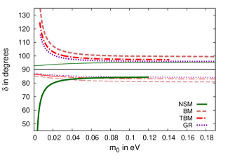
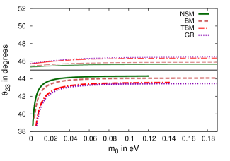
Figure 2: In the left (right) panel the CP-phase $\delta$ ($\theta_{23}$) predicted by this model is plotted as a function of the lightest neutrino mass $m_{0}$ for all the four mixing patterns when the best-fit values of the data are taken as input. The NSM, BM, TBM and GR mixing alternatives are represented by the green solid, pink dashed, red dot-dashed, and violet dotted curves respectively. Thick (thin) curves of each kind denote NO (IO).

From Table 4, it is obvious that $(\epsilon-\theta_{12}^{0})$ exists in the first (fourth) quadrant for the NSM (BM, TBM, and GR) mixing pattern. From Eq. (41) one can immediately conclude that for NSM (BM, TBM, and GR) case(s) $\delta$ remains in the first or fourth (second or third) quadrants in case of normal ordering. $\kappa_{c}$ changes sign for inverted ordering. Thus the quadrants get modified accordingly. The different alternatives are furnished in Table 5. There are two allowed quadrants of $\delta$ having $\sin\delta$ of opposite sign for any mixing option and ordering of neutrino masses. The sign of the right-hand-side of Eq. (42) governs the phases $\phi_{1,2}$ which in its turn decides the quadrants CP-phase $\delta$ out of the two allowed options. As already discussed, $\phi_{2}$ can be in either the first or fourth quadrants. The quadrant of $\phi_{1}$ depends on the mixing pattern in such a manner that $\sin\phi_{1}$ can be of either sign. Therefore, the phases $\phi_{1}$ and $\phi_{2}$ can be chosen in a way such that $\sin\delta$ can acquire any particular sign. Thus the two alternate quadrants of $\delta$ for every case in Table 5 are equally allowed in the model.

The Type-I see-saw perturbative contribution to the atmospheric mixing angle can be obtained from Eq. (39) as:

$$\tan\omega=\frac{\sin\theta_{13}\cos\delta}{\tan(\epsilon-\theta_{12}^{0})}\;.$$ (43)

Let us recall, Eq. (41) relates $\delta$ and $(\epsilon-\theta_{12}^{0})$ through $\kappa_{c}$. Thus for all mixing alternatives $~{}\theta_{23}$ always remains in first (second) octant for NO (IO). This is one of the most important results of the model as shown in Table 5.

In the solar splitting expressed in Eq. (38), the factor of  $m_{D}^{2}/m_{R}$ can be replaced in terms of $\kappa_{c}$. This together with Eq. (41) gives,

$$\Delta m^{2}_{solar}=\frac{2m^{-}m_{1}^{(0)}\sin\theta_{13}\cos\delta\cos\epsilon}{\sin(\epsilon-\theta_{12}^{0})\ cos2\zeta}\;.$$ (44)

Predictions of the model can be extracted from Eqs. (43) and (44). The three mixing angles $\theta_{13}$, $\theta_{12}$, and $\theta_{23}$ are taken as inputs. Eq. (43) determines a value of the CP-violating phase $\delta$. With the help of these and the experimentally observed solar splitting the combination $m_{1}^{(0)}m^{-}$, or equivalently the variable $z$ can be calculated using Eq. (44) that fixes the lightest neutrino mass $m_{0}$. It may seem that arbitrarily large values of $m_{0}$, and hence $m_{1}^{(0)}m^{-}$, may be accounted for by tuning $\cos\delta$ to smaller and smaller values. However, this certainly is not the case. Experimental data necessitate $\omega=(\pi/4-\theta_{23})$ to be restricted within observed limits. As all other factors have ranges determined experimentally, Eq. (43) also puts lower and upper bounds on $\delta$. Subsequently, $m_{0}$ lies within a fixed range for any mixing pattern.

Fig. 2 contains the CP-phase $\delta$ ($\theta_{23}$) as a function of the lightest neutrino mass $m_{0}$ for different mixing patterns as predicted by this model in the left (right) panel while the best-fit values of the various measured angles and mass splittings are used. The NSM, BM, TBM and GR are depicted by green solid, pink dashed, red dot-dashed, and violet dotted curves respectively. The thick (thin) curves of each kind indicate NO (IO). Normal and inverted orderings are always associated with the first and second octants of the atmospheric mixing angle $\theta_{23}$ respectively. For NSM case $\delta$ lies in the first (second) quadrant for normal (inverted) ordering, while for the rest of the mixing options it is in the second (first) quadrant. For inverted neutrino mass ordering $|\delta|$ remains close to $\pi/2$ for the complete range of $m_{0}$. The CP-phase $\delta$ lies near $\pi/2$ for normal ordering for $m_{0}$ larger than around 0.05 eV.

From Table 5 it is evident that if $\delta$ is a solution for some $m_{0}$ then by properly choosing alternate values of the phases $\phi_{1,2}$ appearing in $M_{\nu R}$ one can also obtain a second solution with the phase $-\delta$. This mirror set of solutions are not shown in Fig. 2. The preliminary data presented by the T2K [21] and NOVA [22] collaborations can be considered as primary hint of normal ordering associated with $\delta\sim-\pi/2$. The consistency of this model with these observations is clearly visible from Fig. 2 with $\delta\sim-\pi/2$ favouring $m_{0}$ in the quasi-degenerate regime, i.e., $m_{0}\geq\mathcal{O}$(0.05 eV), for normal ordering. If this result is determined with better accuracy in the future analysis then the model will predict neutrino masses to be in a range that ongoing experiments are capable of probing [23, 24].

These interrelationships between the octant of $\theta_{23}$, the quadrant of the CP-violating phase $\delta$, and the neutrino mass ordering provide a clear set of correlations characteristic of this $A4$ based model. In the model the corrections to the three neutrino mixing angles and $\Delta m^{2}_{solar}$ all have a common origin – the Type-I see-saw. As a result these parameters get correlated. Such interrelationships are specific to this model. Although the model has a large number of parameters, only this correlated region of the parameter space allowed by neutrino mass and mixing data leads to testable predictions in Table 5.

V Conclusions

In this paper an $A4$ based see-saw model for neutrino masses and mixing has been proposed. The flavour quantum numbers suitable for the model are assigned to the leptons and the scalars. The Lagrangian is inclusive of all the symmetry conserving terms. No soft breaking of symmetry is entertained. The Yukawa couplings induce the charged lepton masses, Dirac and Majorana masses for the left- and right-handed neutrinos after the symmetry is broken spontaneously. Neutrino masses are produced by a combined effect of both Type-I and Type-II see-saw terms present in the Lagrangian of which the former can be thought of to be a small correction. The Type-II see-saw dominant contribution is associated with the atmospheric mass splitting, no solar splitting, keeps $\theta_{23}=\pi/4$, and $\theta_{13}=0$ and $\theta_{12}$ can be given any preferred value. In particular, this model is scrutinized in context of tribimaximal, bimaximal, golden ratio, and ‘no solar mixing’ patterns. The contribution of Type-I see-saw can be treated as a perturbation that generates the solar splitting and tunes the mixing angles to values in agreement with the global fits. As a corollary a correlation between the octants of $\theta_{23}$ and neutrino mass ordering followed – first (second) octant is allowed for normal (inverted) ordering of neutrino mass. The model has several testable predictions including that of the CP-phase $\delta$, relationships between mixing angles and mass splittings. Moreover, inverted ordering got associated with near-maximal CP-phase $\delta$ and arbitrarily small neutrino masses are allowed. In case of normal ordering $\delta$ can vary over a larger range and maximality is accomplished in the quasi-degenerate regime. The lightest neutrino mass has to be at least a few meV for this case.

Acknowledgements: I acknowledge support from CSIR, India during the initial stage of this work at University of Calcutta. I also thank Prof. Amitava Raychaudhuri for his valuable insights and comments at various stages of this endeavor.

A Appendix: The group $A4$

$A4$ is the even permutation group of four objects having 12 elements and two generators $S$ and $T$ satisfying the property $S^{2}=T^{3}=(ST)^{3}=\mathbb{I}$. It has four inequivalent irreducible representations viz. one 3 dimensional representation and three 1 dimensional representations namely, $1,1^{\prime}$ and $1^{\prime\prime}$. These three dimension-1 representations are singlets under $S$ whereas they transform as 1, $\omega$, and $\omega^{2}$ respectively under the action of $T$, $\omega$ being a cube root of unity. Therefore it is apparent that $1^{\prime}\times 1^{\prime\prime}=1$. The pertinent form of the generators $S$ and $T$ acting on the 3 dimensional representations are given by,

$$S=\pmatrix{1&0&0\cr 0&-1&0\cr 0&0&-1}\ \ \ \ {\rm and}\ \ \ \ T=\pmatrix{0&1&0\cr 0&0&1\cr 1&0&0}\;\;.$$ (A.1)

It is imperative to note the product rule for the three dimensional representation is:

$$3\otimes 3=1\oplus 1^{\prime}\oplus 1^{\prime\prime}\oplus 3\oplus 3\;\;.$$ (A.2)

When two triplets of $A4$ given by $3_{a}\equiv{a_{i}}$ and $3_{b}\equiv{b_{i}}$, with $i=1,2,3$; are combined according to Eq. (A.2), then the resultant triplets can be represented by $3_{c}\equiv{c_{i}}$ and $3_{d}\equiv{d_{i}}$ where,

$$c_{i} = \left(\frac{a_{2}b_{3}+a_{3}b_{2}}{2},\frac{a_{3}b_{1}+a_{1}b_{3}}{2},\frac{a_{1}b_{2}+a_{2}b_{1}}{2}\right)\;\;,\;\;{\rm or,}\;\;c_{i}\equiv\alpha_{ijk}a_{j}b_{k}\;\;,$$

$$d_{i} = \left(\frac{a_{2}b_{3}-a_{3}b_{2}}{2},\frac{a_{3}b_{1}-a_{1}b_{3}}{2},\frac{a_{1}b_{2}-a_{2}b_{1}}{2}\right)\;\;,\;\;{\rm or,}\;\;d_{i}\equiv\beta_{ijk}a_{j}b_{k}\;\;,\;\;(i,j,k,{\rm are~{}cyclic})\;\;.$$ (A.3)

and the $1$, $1^{\prime}$ and $1^{\prime\prime}$ so obtained can be scripted as:

$$1 = a_{1}b_{1}+a_{2}b_{2}+a_{3}b_{3}\equiv\rho_{1ij}a_{i}b_{j}\;\;,$$

$$1^{\prime} = a_{1}b_{1}+\omega^{2}a_{2}b_{2}+\omega a_{3}b_{3}\equiv\rho_{3ij}a_{i}b_{j}\;\;,$$

$$1^{\prime\prime} = a_{1}b_{1}+\omega a_{2}b_{2}+\omega^{2}a_{3}b_{3}\equiv\rho_{2ij}a_{i}b_{j}\;\;.$$ (A.4)

The group is studied in extensive details in [9, 10].

B Appendix: Minimization of the scalar potential

Some detailed analysis of the nature of the scalar potential is presented in this Appendix. The conditions that have to be satisfied by the parameters of the potential so that the vevs acquire the values considered in the model are extracted. The conditions so obtained guarantee the potential is locally minimized by those choices. To confirm if those choices are in concurrence with the global minimum is beyond the scope of this work.

The fields catalogued in Table 3 comprise of scalars having lepton numbers as well as $A4$, $SU(2)_{L}$, and $U(1)_{Y}$ charges. The scalar potential must be of the most general quartic nature conserving all the symmetries under consideration. Thus all the terms allowed by the symmetries are included in the discussion below. Verification of $SU(2)_{L}$, $U(1)_{Y}$ and lepton number are familiar exercises. $A4$ invariance requires elaborate discussion as presented in the following section.

B.1 $A4$ conserving terms: Notations and general principles

Let us summarize a few salient features of this model to fix the notations to be followed for the $A4$-invariant terms. As already noted, the scalar spectrum has fields transforming as $1,1^{\prime},1^{\prime\prime},$ and $3$ under $A4$. One has to consider all the combinations of these fields up to quartics that can yield $A4$ invariants. The product rules for $1,1^{\prime}$ and $1^{\prime\prime}$ are easy, but that for the triplets of $A4$ needs to be emphasized. If there are two $A4$ triplet fields $A\equiv(a_{1},a_{2},a_{3})^{T}$ and $B\equiv(b_{1},b_{2},b_{3})^{T}$ where $a_{i},b_{i}$ may possess $SU(2)_{L}\times U(1)_{Y}$ transformation properties that are not considered for the time being in the immediate course of discussion. As furnished in Eq. (A.2), one can combine $A$ and $B$ to obtain

$$3_{A}\otimes 3_{B}=1\oplus 1^{\prime}\oplus 1^{\prime\prime}\oplus 3\oplus 3\;\;.$$ (B.1)

For notational simplicity let us denote the irreducible representations on the right-hand-side by $O_{1}(A,B)$, $O_{2}(A,B)$, $O_{3}(A,B)$, $T_{s}(A,B)$ and $T_{a}(A,B)$, respectively, where, as already noted in Eqs. (A.3, A.4)

$$O_{1}(A,B) \equiv 1=a_{1}b_{1}+a_{2}b_{2}+a_{3}b_{3}\equiv\rho_{1ij}a_{i}b_{j}\;\;,$$

$$O_{2}(A,B) \equiv 1^{\prime}=a_{1}b_{1}+\omega^{2}a_{2}b_{2}+\omega a_{3}b_{3}\equiv\rho_{3ij}a_{i}b_{j}\;\;,$$

$$O_{3}(A,B) \equiv 1^{\prime\prime}=a_{1}b_{1}+\omega a_{2}b_{2}+\omega^{2}a_{3}b_{3}\equiv\rho_{2ij}a_{i}b_{j}\;\;,$$ (B.2)

and

$$T_{s}(A,B) \equiv 3=\left(\frac{a_{2}b_{3}+a_{3}b_{2}}{2},\ \ \frac{a_{3}b_{1}+a_{1}b_{3}}{2},\ \ \frac{a_{1}b_{2}+a_{2}b_{1}}{2}\right)^{T}\;\;,$$

$$T_{a}(A,B) \equiv 3=\left(\frac{a_{2}b_{3}-a_{3}b_{2}}{2},\ \ \frac{a_{3}b_{1}-a_{1}b_{3}}{2},\ \ \frac{a_{1}b_{2}-a_{2}b_{1}}{2}\right)^{T}\;\;.$$ (B.3)

It is worth noticing that $O_{3}(A^{\dagger},A)=[O_{2}(A^{\dagger},A)]^{\dagger}$ and $T_{a}(A,A)=0$.

The scalar potential can be formulated implementing this notation and keeping in mind that the scalar sector of this model is devoid of any field which is invariant under all the symmetries under consideration. Therefore the scalar potential will contain terms of the following kind (only $A4$ properties are exhibited):

1. Quadratic: $W^{\dagger}W$,

2. Cubic: $X_{i}X^{\prime}_{j}X^{\prime\prime}_{k},X_{i}X_{j}X_{k}$, $X^{\prime}_{i}X^{\prime}_{j}X^{\prime}_{k},$ $X^{\prime\prime}_{i}X^{\prime\prime}_{j}X^{\prime\prime}_{k}$, $O_{1}(Y_{i},Y_{j})X_{k}$, $O_{2}(Y_{i},Y_{j})X^{\prime\prime}_{k}$, $O_{3}(Y_{i},Y_{j})X^{\prime}_{k}$,

3. Quartic: $(W_{i}^{\dagger}W_{i})(W_{j}^{\dagger}W_{j}),~{}(X_{i}X_{j})(X_{k}X_{l}),~{}(X_{i}X_{j})(X^{\prime}_{k}X^{\prime\prime}_{l}),~{}(X^{\prime}_{i}X^{\prime\prime}_{j})(X^{\prime}_{k}X^{\prime\prime}_{l}),~{}(X^{\prime}_{i}X^{\prime}_{j})(X^{\prime}_{k}X_{l}),~{}(X^{\prime\prime}_{i}X^{\prime\prime}_{j})(X^{\prime\prime}_{k}X_{l})$,
   $O_{1}(Y_{i},Y_{j})X_{k}X_{l},~{}O_{1}(Y_{i},Y_{j})X^{\prime}_{k}X^{\prime\prime}_{l},~{}O_{2}(Y_{i},Y_{j})X^{\prime}_{k}X^{\prime}_{l},~{}O_{2}(Y_{i},Y_{j})X_{k}X^{\prime\prime}_{l}$,
   $O_{3}(Y_{i},Y_{j})X^{\prime\prime}_{k}X^{\prime\prime}_{l},~{}O_{3}(Y_{i},Y_{j})X_{k}X^{\prime}_{l}$,
   $O_{1}(Y_{i},Y_{j})O_{1}(Y_{k},Y_{l}),O_{2}(Y_{i},Y_{j})^{\dagger}O_{2}(Y_{k},Y_{l}),O_{3}(Y_{i},Y_{j})^{\dagger}O_{3}(Y_{k},Y_{l}),O_{2}(Y_{i},Y_{j})O_{3}(Y_{k},Y_{l})$,
   $O_{1}(T_{s}(Y_{i},Y_{j}),T_{s}(Y_{k},Y_{l}))$, $O_{1}(T_{s}(Y_{i},Y_{j}),T_{a}(Y_{k},Y_{l}))$, $O_{1}(T_{a}(Y_{i},Y_{j}),T_{a}(Y_{k},Y_{l}))$.
   $O_{1}(T_{s}(Y_{i},Y_{j}),Y_{k})X_{l}$, $O_{2}(T_{s}(Y_{i},Y_{j}),Y_{k})X^{\prime\prime}_{l}$, $O_{3}(T_{s}(Y_{i},Y_{j}),Y_{k})X^{\prime}_{l}$,
   $O_{1}(T_{a}(Y_{i},Y_{j}),Y_{k})X_{l}$, $O_{2}(T_{a}(Y_{i},Y_{j}),Y_{k})X^{\prime\prime}_{l}$, $O_{3}(T_{a}(Y_{i},Y_{j}),Y_{k})X^{\prime}_{l}$ .

Here $W$ is any field, $X$, $X^{\prime}$, and $X^{\prime\prime}$ represent generic fields transforming as $1$, $1^{\prime}$, and $1^{\prime\prime}$ under $A4$ while $Y$ happens to be generic $A4$ triplet field. The invariants constructed by using $X^{\dagger}$, $X^{\prime\dagger}$, $X^{\prime\prime\dagger}$, and $Y^{\dagger}$ are not listed separately.

Owing to the large number of scalars in the model – e.g., $SU(2)_{L}$ singlets, doublets, and triplets – the scalar potential consists of many terms. In order to simplify the discussion, cubic terms in the fields are excluded and all the couplings are taken to be real. The antisymmetric triplet arising from the combination of two $A4$ triplets i.e., the terms denoted by $T_{a}$ in Eq. (B.3) are not included in the potential throughout for ease of calculation. The potential is studied piece-wise: (a) consisting of terms that arise from combination of fields belonging to same $SU(2)_{L}$ sector, and (b) comprising of terms obtained by combining scalars of different $SU(2)_{L}$ sectors. The vev of the $SU(2)_{L}$ singlets giving rise to the right-handed neutrino mass are larger than the vev of the other scalar fields. Thus in the latter category the combinations of $SU(2)_{L}$ singlets with the doublets and triplets of $SU(2)_{L}$ are considered, whereas, doublet-triplet inter-sector terms are dropped owing to the smallness of the triplet vev responsible for the left-handed Majorana neutrino mass. Also the electroweak precision measurements put a stringent bound on the triplet vev compelling it to be very small.

B.2 $SU(2)_{L}$ Singlet Sector:

The $SU(2)_{L}$ singlet scalar sector consists of three $A4$ triplets $\hat{\Delta}^{R}_{p}$ with $p=a,b,c$ denoting each one of them. These three triplets possess identical quantum numbers, their vev being the only discriminating criterion. Also there are three more fields viz. $\Delta_{1}^{R}$, $\Delta_{2}^{R}$ and $\Delta_{3}^{R}$ transforming as $1$, $1^{\prime}$ and $1^{\prime\prime}$ under $A4$. From Eq. (B.1) we can see that two same $\hat{\Delta}^{R}_{p}$ triplets can combine to produce several $A4$ irreducible representations. For notational simplicity let us define:

$$O_{1p}^{ss}\equiv O_{1}(\hat{\Delta}^{R\dagger}_{p},\hat{\Delta}^{R}_{p});~{}O_{2p}^{ss}\equiv O_{2}(\hat{\Delta}^{R\dagger}_{p},\hat{\Delta}^{R}_{p});~{}T_{sp}^{ss}\equiv T_{s}(\hat{\Delta}^{R}_{p},\hat{\Delta}^{R}_{p})\;\;,\;\;(p=a,b,c).$$ (B.4)

Using two different triplets $\hat{\Delta}^{R}_{p}$ and $\hat{\Delta}^{R}_{q}$ where $p\neq q$ analogous combinations can be defined:

$$\hat{O}_{1pq}^{ss}\equiv O_{1}(\hat{\Delta}^{R\dagger}_{p},\hat{\Delta}^{R}_{q});~{}\hat{O}_{2pq}^{ss}\equiv O_{2}(\hat{\Delta}^{R\dagger}_{p},\hat{\Delta}^{R}_{q});~{}\hat{T}_{spq}^{ss}\equiv T_{s}(\hat{\Delta}^{R}_{p},\hat{\Delta}^{R}_{q})\;\;,\;\;(p,q=a,b,c\ \ {\rm and}\ \ p\neq q).$$ (B.5)

Generically, it is convenient to use $\widetilde{O}_{ip}$ or $\widetilde{T}_{sp}$ if the second triplet in the argument is replaced by its hermitian conjugate. As an example,

$$~{}\widetilde{O}_{1p}^{ss}\equiv O_{1}(\hat{\Delta}^{R\dagger}_{p},\hat{\Delta}^{R\dagger}_{p}),~{}\widetilde{O}_{2p}^{ss}\equiv O_{2}(\hat{\Delta}^{R\dagger}_{p},\hat{\Delta}^{R\dagger}_{p}),~{}\widetilde{O}_{3p}^{ss}\equiv O_{3}(\hat{\Delta}^{R\dagger}_{p},\hat{\Delta}^{R\dagger}_{p})~{}{\rm and}~{}\widetilde{T}_{sp}^{ss}\equiv T_{s}(\hat{\Delta}^{R}_{p},\hat{\Delta}^{R\dagger}_{p}),$$ (B.6)

One can also consider:

$$~{}\widetilde{O}_{1pq}^{ss}\equiv O_{1}(\hat{\Delta}^{R\dagger}_{p},\hat{\Delta}^{R\dagger}_{q}),~{}\widetilde{O}_{2pq}^{ss}\equiv O_{2}(\hat{\Delta}^{R\dagger}_{p},\hat{\Delta}^{R\dagger}_{q}),~{}\widetilde{O}_{3pq}^{ss}\equiv O_{3}(\hat{\Delta}^{R\dagger}_{p},\hat{\Delta}^{R\dagger}_{q}).$$ (B.7)

Also the following combinations are required:

$$~{}\mathscr{O}_{1p}^{ss}\equiv O_{1}(\hat{\Delta}^{R}_{p},{T}_{sp}^{ss\dagger}),~{}\mathscr{O}_{2p}^{ss}\equiv O_{2}(\hat{\Delta}^{R}_{p},{T}_{sp}^{ss\dagger}),~{}\mathscr{O}_{3p}^{ss}\equiv O_{3}(\hat{\Delta}^{R}_{p},{T}_{sp}^{ss\dagger})\;\;,\;\;(p=a,b,c).$$ (B.8)

The $A4$ singlets $\Delta_{i}^{R}$ ($i=1,2,3$) can be combined to yield

$$Q_{i}^{ss}\equiv\Delta_{i}^{R\dagger}\Delta_{i}^{R}\;\;,\;\;(i=1,2,3).$$ (B.9)

Needless to mention that such terms are singlets of all the symmetries under consideration.

Having devised the essential notations one can write the most general scalar potential for the $SU(2)_{L}$ singlet sector of this model as:

$$V_{singlet} = \sum_{i=1}^{3}m_{\Delta_{i}^{R}}^{2}Q_{i}^{ss}+\sum_{p=a}^{c}m_{\hat{\Delta}^{R}_{p}}^{2}O_{1p}^{ss}+\left[\sum_{{p\neq q};\,{p,q=a}}^{c}m_{\hat{\Delta}^{R}_{pq}}^{2}\hat{O}_{1pq}^{ss}\ \ +\ \ {\rm all}\ \ {\rm possible}\ \ {\rm permutations}\right]$$

$$+ {1\over 2}\sum_{i=1}^{3}\lambda^{s}_{1i}\left[Q_{i}^{ss}\right]^{2}+{1\over 2}\sum_{k<j;\,k\neq j;\,k=1}^{2}\sum_{j=2}^{3}\lambda^{s}_{2jk}\left\{Q_{j}^{ss}Q_{k}^{ss}\right\}$$

$$+ {1\over 2}\sum_{p=a}^{c}\lambda_{3p}^{s}\left\{[O_{1p}^{ss}]^{2}+(O_{2p}^{ss})^{\dagger}O_{2p}^{ss}+O_{1p}({T_{sp}^{ss}},T_{sp}^{ss\dagger})\right\}$$

$$+ \sum_{{p\neq q};\,{p,q=a}}^{c}\lambda^{s}_{3pq}\left\{[\hat{O}_{1pq}^{ss}]^{2}+(\hat{O}_{2pq}^{ss})^{\dagger}\hat{O}_{2pq}^{ss}+h.c.\right\}+{1\over 2}\sum_{{p\neq q};\,{p,q=a}}^{c}\widetilde{\lambda}^{s}_{3pq}\left\{(\hat{O}_{1pq}^{ss})^{\dagger}\hat{O}_{1pq}^{ss}+O_{1}({\hat{T}_{spq}^{ss}},\hat{T}_{spq}^{ss\dagger})\right\}$$

$$+ \sum_{p=a}^{c}\sum_{i=1}^{3}\left[{1\over 2}\lambda^{s}_{4ip}\left(Q_{i}^{ss}O_{1p}^{ss}\right)\right]+\sum_{i=1}^{3}\sum_{{p\neq q};\,{p,q=a}}^{c}\lambda^{s}_{4ipq}\left[\left(Q_{i}^{ss}\hat{O}_{1pq}^{ss}\right)+h.c.\right]+{1\over 2}\sum_{p=a}^{c}\lambda^{s}_{5p}\left(\mathscr{O}_{1p}^{ss}\Delta_{1}^{R}+~{}{\rm h.c.}\right)$$

$$+ \sum_{{p\neq q};\,{p,q=a}}^{c}\lambda^{s}_{5pq}\left[\left\{\left(\Delta_{1}^{R}O_{1}(\hat{\Delta}_{p}^{R},\hat{T}_{spq}^{ss\dagger}\right)+\left(\Delta_{1}^{R}O_{1}(\hat{\Delta}_{q}^{R},\hat{T}_{spq}^{ss\dagger}\right)\right\}+h.c.\right]$$

$$+ {1\over 2}\sum_{p=a}^{c}\lambda^{s}_{6p}\left(\mathscr{O}_{3p}^{ss}\Delta_{2}^{R}+~{}{\rm h.c.}\right)+\sum_{{p\neq q};\,{p,q=a}}^{c}\lambda^{s}_{6pq}\left[\left\{\left(\Delta_{2}^{R}O_{3}(\hat{\Delta}_{p}^{R},\hat{T}_{spq}^{ss\dagger}\right)+\left(\Delta_{2}^{R}O_{3}(\hat{\Delta}_{q}^{R},\hat{T}_{spq}^{ss\dagger}\right)\right\}+h.c.\right]$$

$$+ {1\over 2}\sum_{p=a}^{c}\lambda^{s}_{7p}\left(\mathscr{O}_{2p}^{ss}\Delta_{3}^{R}+~{}{\rm h.c.}\right)+\sum_{{p\neq q};\,{p,q=a}}^{c}\lambda^{s}_{7pq}\left[\left\{\left(\Delta_{3}^{R}O_{2}(\hat{\Delta}_{p}^{R},\hat{T}_{spq}^{ss\dagger}\right)+\left(\Delta_{3}^{R}O_{2}(\hat{\Delta}_{q}^{R},\hat{T}_{spq}^{ss\dagger}\right)\right\}+h.c.\right]$$

$$+ \sum_{p=a}^{c}\sum_{i=1}^{3}\lambda^{s}_{8ip}\left({\Delta_{i}^{R}}^{2}\widetilde{O}_{ip}+h.c.\right)+\sum_{{p\neq q};\,{p,q=a}}^{c}\sum_{i=1}^{3}\lambda^{s}_{8ipq}\left({\Delta_{i}^{R}}^{2}\widetilde{O}_{ipq}+h.c.\right)$$

$$+ \sum_{p=a}^{c}\left[\lambda^{s}_{91p}\Delta_{2}^{R}\Delta_{3}^{R}\widetilde{O}_{1p}+\lambda^{s}_{92p}\Delta_{1}^{R}\Delta_{3}^{R}\widetilde{O}_{2p}+\lambda^{s}_{93p}\Delta_{1}^{R}\Delta_{2}^{R}\widetilde{O}_{3p}+h.c.\right]$$

$$+ \sum_{{p\neq q};\,{p,q=a}}^{c}\left[\lambda^{s}_{91pq}\Delta_{2}^{R}\Delta_{3}^{R}\widetilde{O}_{1pq}+\lambda^{s}_{92pq}\Delta_{1}^{R}\Delta_{3}^{R}\widetilde{O}_{2pq}+\lambda^{s}_{93pq}\Delta_{1}^{R}\Delta_{2}^{R}\widetilde{O}_{3pq}+h.c.\right].$$

$$\;\;.$$ (B.10)

Here $\lambda^{s}_{3p}$, $\lambda^{s}_{3pq}$ and $\widetilde{\lambda}^{s}_{3pq}$ are taken as the common coefficient of the different $A4$ invariants generated by combining two $\hat{\Delta}^{R}$ and two $(\hat{\Delta}^{R})^{\dagger}$ fields. Similar policy will be adopted for the fields with other $SU(2)_{L}$ properties.

B.3 $SU(2)_{L}$ Doublet Sector:

The $SU(2)_{L}$ doublet scalar precinct consists of the two fields $\Phi$ and $\eta$ transforming as $3$ and $1$ of $A4$ respectively. Opposite hypercharges are assigned to $\Phi$ and $\eta$. The $A4$ triplet $\Phi$ combinations are denoted as:

$$O_{1}^{dd}\equiv O_{1}(\Phi^{\dagger},\Phi);~{}O_{2}^{dd}\equiv O_{2}(\Phi^{\dagger},\Phi);~{}T_{s}^{dd}\equiv T_{s}(\Phi,\Phi),$$ (B.11)

and that of the $A4$ singlet $\eta$ are:

$$Q_{\eta}^{dd}\equiv\eta^{\dagger}\eta\;\;.$$ (B.12)

The potential for the $SU(2)_{L}$ doublet sector is given by:

$$V_{doublet} = m_{\eta}^{2}Q_{\eta}^{dd}+m_{\Phi}^{2}O_{1}^{dd}+{1\over 2}\lambda^{d}_{1}\left[Q_{\eta}^{dd}\right]^{2}+{1\over 2}\lambda^{d}_{2}\left\{[O_{1}^{dd}]^{2}+\{O_{2}^{dd}\}^{\dagger}O_{2}^{dd}\right.$$ (B.13)

$$+ \left.O_{1}({T_{s}^{dd}},T_{s}^{dd\dagger})\right\}+{1\over 2}\lambda^{d}_{3}\left[Q_{\eta}^{dd}O_{1}^{dd}\right].$$

B.4 $SU(2)_{L}$ Triplet Sector:

The $SU(2)_{L}$ triplet sector comprises of five fields. There are two $A4$ triplets $\hat{\Delta}^{L}_{a}$ and $\hat{\Delta}^{L}_{b}$ together with the fields the $\Delta^{L}_{1}$, $\Delta^{L}_{2}$ and $\Delta^{L}_{3}$ transforming as $1$, $1^{\prime}$, $1^{\prime\prime}$ of $A4$ respectively. It is useful to define:

$$O_{1n}^{tt}\equiv O_{1}(\hat{\Delta}^{L\dagger}_{n},\hat{\Delta}^{L}_{n});~{}O_{2n}^{tt}\equiv O_{2}(\hat{\Delta}^{L\dagger}_{n},\hat{\Delta}^{L}_{n});~{}T_{sn}^{tt}\equiv T_{s}(\hat{\Delta}^{L}_{n},\hat{\Delta}^{L}_{n})\;\;,\;\;(n=a,b),$$ (B.14)

$$\hat{O}_{1nl}^{tt}\equiv O_{1}(\hat{\Delta}^{L\dagger}_{n},\hat{\Delta}^{L}_{l});~{}\hat{O}_{2nl}^{tt}\equiv O_{2}(\hat{\Delta}^{L\dagger}_{n},\hat{\Delta}^{L}_{l});~{}\hat{O}_{3nl}^{tt}\equiv O_{3}(\hat{\Delta}^{L\dagger}_{n},\hat{\Delta}^{L}_{l});~{}\hat{T}_{snl}^{tt}\equiv T_{s}(\hat{\Delta}^{L}_{n},\hat{\Delta}^{L}_{l}),\;\;(n,l=a,b\ \ {\rm and}\ \ n\neq l),$$ (B.15)

$$Q_{i}^{tt}\equiv\Delta_{i}^{L\dagger}\Delta_{i}^{L}\;\;,\;\;(i=1,2,3),$$ (B.16)

and

$$~{}\mathscr{O}_{\gamma n}^{tt}\equiv O_{\gamma}(\hat{\Delta}^{L}_{n},T_{sn}^{tt\dagger});~{}\mathscr{O}_{\gamma nl}^{tt}\equiv O_{\gamma}(\hat{\Delta}^{L}_{n},\hat{T}_{sl}^{tt\dagger}),\;\;(\gamma=1,2,3)\;\;{\rm and}\ \ (n,l=a,b),$$ (B.17)

$$~{}\widetilde{O}^{tt}_{jn}\equiv O_{j}(\hat{\Delta}^{L\dagger}_{n},\hat{\Delta}^{L\dagger}_{n});~{}\widetilde{O}^{tt}_{jnl}\equiv O_{j}(\hat{\Delta}^{L\dagger}_{n},\hat{\Delta}^{L\dagger}_{l}),\;\;(j=1,2,3)\;\;{\rm and}\ \ (n,l=a,b\ \ {\rm and}\ \ n\neq l).$$ (B.18)

The scalar potential for this sector:

$$V_{triplet} = \sum_{i=1}^{3}{m^{2}_{\Delta^{L}_{i}}}~{}Q_{i}^{tt}+\sum_{n=a}^{b}m_{\hat{\Delta}^{L}_{n}}^{2}~{}O_{1n}^{tt}+\left(\sum_{{n\neq l;\,n,l=a}}^{b}m_{\hat{\Delta}^{L}_{nl}}^{2}~{}\hat{O}_{1nl}^{tt}+\ \ {\rm all}\ \ {\rm possible}\ \ {\rm permutations}\right)$$

$$+ {1\over 2}\sum_{i=1}^{3}\lambda^{t}_{1_{i}}\left[Q_{i}^{tt}\right]^{2}+{1\over 2}\sum_{k<j,\,k=1}^{2}\sum_{j=2}^{3}\lambda^{t}_{2jk}Q_{j}^{tt}Q_{k}^{tt}+{1\over 2}\sum_{n=a}^{b}\lambda^{t}_{3n}\left\{[O_{1n}^{tt}]^{2}+\{O_{2n}^{tt}\}^{\dagger}O_{2n}^{tt}+O_{1}({T_{sn}^{tt}},T_{sn}^{tt\dagger})\right\}$$

$$+ {1\over 2}\sum_{{n\neq l;\,n,l=a}}^{b}\lambda^{t}_{3nl}\left\{[\hat{O}_{1nl}^{tt}]^{2}+\{\hat{O}_{2nl}^{tt}\}^{\dagger}\hat{O}_{2nl}^{tt}+h.c.\right\}+{1\over 2}\sum_{{n\neq l;\,n,l=a}}^{b}\widetilde{\lambda}^{t}_{3nl}\left\{[\hat{O}_{1nl}^{tt}]^{\dagger}\hat{O}_{1nl}^{tt}]+O_{1}(\hat{T}_{sn}^{tt},\hat{T}_{sn}^{tt\dagger})\right\}$$

$$+ {1\over 2}\sum_{j=1}^{3}\sum_{n=a}^{b}\lambda^{t}_{4_{jn}}\left[\left(\Delta^{L\dagger}_{j}\Delta^{L}_{j}\right)O_{1n}^{tt}\right]+\sum_{j=1}^{3}\sum_{{n\neq l;\,n,l=a}}^{b}\lambda^{t}_{4_{1nl}}\left[\left(\Delta^{L\dagger}_{j}\Delta^{L}_{j}\right)\hat{O}_{1n}^{tt}+h.c.\right]$$

$$+ {1\over 2}\sum_{n=a}^{b}\lambda^{t}_{5n}\left[\left\{\Delta_{1}^{L}\mathscr{O}^{tt}_{1n}\right\}+h.c.\right]+\sum_{{n,l=a}}^{b}\lambda^{t}_{5nl}\left[\left\{\Delta_{1}^{L}\mathscr{O}^{tt}_{1nl}\right\}+h.c.\right]+{1\over 2}\sum_{n=a}^{b}\lambda^{t}_{6n}\left[\left\{\Delta_{2}^{L}\mathscr{O}^{tt}_{3n}\right\}+h.c.\right]$$

$$+ \sum_{{n,l=a}}^{b}\lambda^{t}_{6nl}\left[\left\{\Delta_{2}^{L}\mathscr{O}^{tt}_{3nl}\right\}+h.c.\right]+{1\over 2}\sum_{n=a}^{b}\lambda^{t}_{7n}\left[\left\{\Delta_{3}^{L}\mathscr{O}^{tt}_{2n}\right\}+h.c.\right]+\sum_{{n,l=a}}^{b}\lambda^{t}_{7nl}\left[\left\{\Delta_{3}^{L}\mathscr{O}^{tt}_{2nl}\right\}+h.c.\right]$$

$$+ \sum_{n=a}^{b}\sum_{j=1}^{3}\lambda^{t}_{8jn}\left[\left({\Delta_{j}^{L}}^{2}\widetilde{O}^{tt}_{jn}\right)+h.c.\right]+\sum_{{n\neq l;\,n,l=a}}^{b}\sum_{j=1}^{3}\lambda^{t}_{8jnl}\left[\left({\Delta_{j}^{L}}^{2}\widetilde{O}^{tt}_{jnl}\right)+h.c.\right]$$

$$+ \sum_{n=a}^{b}\left[\left\{\lambda^{t}_{91n}\left(\Delta_{2}^{L}\Delta_{3}^{L}\widetilde{O}^{tt}_{1n}\right)\right\}+\left\{\lambda^{t}_{92n}\left(\Delta_{1}^{L}\Delta_{3}^{L}\widetilde{O}^{tt}_{2n}\right)\right\}+\left\{\lambda^{t}_{93n}\left(\Delta_{1}^{L}\Delta_{2}^{L}\widetilde{O}^{tt}_{3n}\right)\right\}+h.c.\right]$$

$$+ \sum_{{n\neq l;\,n,l=a}}^{b}\left[\left\{\lambda^{t}_{91nl}\left(\Delta_{2}^{L}\Delta_{3}^{L}\widetilde{O}^{tt}_{1nl}\right)\right\}+\left\{\lambda^{t}_{92nl}\left(\Delta_{1}^{L}\Delta_{3}^{L}\widetilde{O}^{tt}_{2nl}\right)\right\}+\left\{\lambda^{t}_{93nl}\left(\Delta_{1}^{L}\Delta_{2}^{L}\widetilde{O}^{tt}_{3nl}\right)\right\}+h.c.\right]$$

$$\;\;.$$ (B.19)

B.5 Inter-sector terms in the scalar potential:

The terms in the scalar potential involving scalar fields of identical $SU(2)_{L}$ behavior are already taken into account. Apart from them, the scalar potential will also receive contributions from terms generated by combining scalars of two different $SU(2)_{L}$ sectors that constitute the main objective of the following discussion. In this category the combinations of the $SU(2)_{L}$ singlet scalars with that belonging to either of the doublet or the triplet sector. The other variety of inter-sector terms – doublet-triplet type – are not included. This seems to be a reasonable approximation as the vevs of the singlet fields are the largest.

B.5.1 Singlet-Doublet inter-sector terms:

Let us consider the combinations:

$$\widetilde{T}_{sp}^{ss}\equiv T_{s}(\hat{\Delta}^{R}_{p},\hat{\Delta}^{R\dagger}_{p});\ \ \widetilde{T}_{spq}^{ss}\equiv T_{s}(\hat{\Delta}^{R}_{p},\hat{\Delta}^{R\dagger}_{q})\;\;{\rm and}\;\;\widetilde{T}_{s}^{dd}\equiv T_{s}(\Phi,\Phi^{\dagger}),\ \ (p,q=a,b,c\ \ {\rm and}\ \ p\neq q)$$ (B.20)

and

$$O_{1sp}^{sd}\equiv O_{1}(\widetilde{T}_{s}^{dd},\widetilde{T}_{sp}^{ss});\ \ \hat{O}_{1spq}^{sd}\equiv O_{1}(\widetilde{T}_{s}^{dd},\widetilde{T}_{spq}^{ss});~{}\mathscr{O}_{p\gamma}^{sd}\equiv O_{\gamma}(\hat{\Delta}^{R}_{p},\widetilde{T}_{s}^{dd})\ \ ,\ \ (\gamma=1,2,3)\ \ {\rm and}\ \ (p,q=a,b,c\ \ {\rm with}\ \ p\neq q).$$ (B.21)

Using this notations:

$$V_{sd} = {1\over 2}\sum_{i=1}^{3}\left[\lambda^{sd}_{1i}\left(Q_{i}^{ss}Q_{\eta}^{dd}\right)+\left(\lambda^{sd}_{2i}Q_{i}^{ss}O_{1}^{dd}\right)\right]+{1\over 2}\sum_{p=a}^{c}\lambda^{sd}_{3p}\left[Q_{\eta}^{dd}O_{1p}^{ss}\right]+{1\over 2}\sum_{{p\neq q};\,{p,q=a}}^{c}\left[Q_{\eta}^{dd}\hat{O}^{ss}_{1pq}\right]$$ (B.22)

$$+ \sum_{p=a}^{c}\left[\lambda^{sd}_{4p}\left(\{\mathscr{O}_{1p}^{sd}\}\Delta_{1}^{R}+h.c.\right)+\lambda^{sd}_{5p}\left(\{\mathscr{O}_{2p}^{sd}\}\Delta_{2}^{R}+h.c.\right)+\lambda^{sd}_{6p}\left(\{\mathscr{O}_{3p}^{sd}\}\Delta_{3}^{R}+h.c.\right)\right]$$

$$+ {1\over 2}\sum_{p=a}^{c}\lambda^{sd}_{7p}\left[O_{1}^{dd}O_{1p}^{ss}+\{O_{2p}^{ss}\}^{\dagger}O_{2}^{dd}+\{O_{2}^{dd}\}^{\dagger}O_{2p}^{ss}+O_{1sp}^{sd}\right]$$

$$+ {1\over 2}\sum_{{p\neq q};\,{p,q=a}}^{c}\lambda^{sd}_{7pq}\left[O_{1}^{dd}\hat{O}_{1pq}^{ss}+\{\hat{O}_{2pq}^{ss}\}^{\dagger}O_{2}^{dd}+\{O_{2}^{dd}\}^{\dagger}\hat{O}_{2pq}^{ss}+\hat{O}_{1spq}^{sd}\right].$$

In the last two terms a simplifying assumption of using a common couplings $\lambda_{7p}^{sd}$ and $\lambda_{7pq}^{sd}$ for the terms in the scalar potential that are generated from various combinations of $(\Phi^{\dagger}\Phi)(\hat{\Delta}^{R\dagger}\hat{\Delta}^{R})$, all four of the fields involved being triplets of $A4$.

B.5.2 Singlet-Triplet inter-sector terms:

In this case the following combinations comes into play:

$$\widetilde{T}^{tt}_{sn} \equiv T_{s}(\hat{\Delta}^{L}_{n},\hat{\Delta}^{L\dagger}_{n});\ \ \widetilde{T}^{tt}_{snl}\equiv T_{s}(\hat{\Delta}^{L}_{n},\hat{\Delta}^{L\dagger}_{l});\ \ O_{1snp}^{ts}\equiv O_{1}(\widetilde{T}^{tt}_{sn},\widetilde{T}^{ss}_{sp});\ \ \hat{O}_{1snpq}^{ts}\equiv O_{1}(\widetilde{T}_{sn}^{tt},\widetilde{T}_{spq}^{ss});\ \$$

$$\hat{O}_{1snlp}^{ts} \equiv O_{1}(\widetilde{T}_{snl}^{tt},\widetilde{T}_{sp}^{ss});\ \ \hat{O}_{1snlpq}^{ts}\equiv O_{1}(\widetilde{T}_{snl}^{tt},\widetilde{T}_{spq}^{ss});\ \ O_{\gamma np}^{ts}\equiv O_{\gamma}(\hat{\Delta}^{R\dagger}_{p},\hat{\Delta}^{L}_{n});\ \ \widetilde{O}_{\gamma np}^{ts}\equiv O_{\gamma}(\hat{\Delta}^{R}_{p},\hat{\Delta}^{L}_{n});$$

$$\mathscr{O}_{\gamma np}^{ts} \equiv O_{\gamma}(\widetilde{T}_{sp}^{ss},\hat{\Delta}^{L}_{n});\ \ \mathscr{\widetilde{O}}_{\gamma np}^{ts}\equiv O_{\gamma}(\widetilde{T}_{sn}^{tt},\hat{\Delta}^{R}_{p});\ \ \hat{\mathscr{O}}_{\gamma npq}^{ts}\equiv O_{\gamma}(\widetilde{T}_{spq}^{ss},\hat{\Delta}^{L}_{n});\ \ \mathscr{\widetilde{O}}_{\gamma nlp}^{ts}\equiv O_{\gamma}(\widetilde{T}_{snl}^{tt},\hat{\Delta}^{R}_{p}).$$

where $\;\;(\gamma=1,2,3);\ \ (p,q=a,b,c)\ \ {\rm and}\ \ (n,l=a,b)$. Needless to mention $p\neq q$ and $n\neq l$.

Following the convention introduced already:

$$O_{\gamma np}^{ts}\equiv O_{\gamma}(\hat{\Delta}^{R\dagger}_{p},\hat{\Delta}^{L}_{n});\ \ \widetilde{O}_{\gamma np}^{ts}\equiv O_{\gamma}(\hat{\Delta}^{R}_{p},\hat{\Delta}^{L}_{n}),\;(\gamma=1,2,3);\ \ (p=a,b,c)\ \ {\rm and}\ \ (n=a,b).$$ (B.24)

The inter-sector potential for this case is given by:

$$V_{ts} = {1\over 2}\sum_{i=1}^{3}\sum_{j=1}^{3}\lambda^{ts}_{1ij}\left[Q_{i}^{ss}Q_{j}^{tt}\right]+{1\over 2}\sum_{j=1}^{3}\sum_{n=a}^{b}\lambda^{ts}_{2jn}\left[\left(Q_{j}^{ss}O_{1n}^{tt}\right)+h.c.\right]+{1\over 2}\sum_{j=1}^{3}\sum_{{n\neq l;\,n,l=a}}^{b}\lambda^{ts}_{2jnl}\left[\left(Q_{j}^{ss}\hat{O}_{1nl}^{tt}\right)+h.c.\right]$$ (B.25)

$$+ {1\over 2}\sum_{i=1}^{3}\sum_{p=a}^{c}\lambda^{ts}_{3ip}\left[Q_{i}^{tt}O_{1p}^{ss}\right]+\sum_{i=1}^{3}\sum_{{p\neq q};\,{p,q=a}}^{c}\lambda^{ts}_{3ipq}\left[Q_{i}^{tt}\hat{O}_{1pq}^{ss}\right]$$

$$+ {1\over 2}\sum_{p=a}^{c}\sum_{n=a}^{b}\lambda^{ts}_{41nnpp}\left[O_{1n}^{tt}O_{1p}^{ss}+\{O_{2p}^{ss}\}^{\dagger}O_{2n}^{tt}+\{O_{2n}^{tt}\}^{\dagger}O_{2p}^{ss}+O_{1snp}^{ts}\right]$$

$$+ {1\over 2}\sum_{{p\neq q};\,{p,q=a}}^{c}\sum_{n=a}^{b}\lambda^{ts}_{42nnpq}\left[O_{1n}^{tt}\hat{O}_{1pq}^{ss}+\{\hat{O}_{2pq}^{ss}\}^{\dagger}O_{2n}^{tt}+\{O_{2n}^{tt}\}^{\dagger}\hat{O}_{2pq}^{ss}+\hat{O}_{1snpq}^{ts}\right]$$

$$+ {1\over 2}\sum_{p=a}^{c}\sum_{{n\neq l;\,n,l=a}}^{b}\lambda^{ts}_{43nlpp}\left[\hat{O}_{1nl}^{tt}O_{1p}^{ss}+\{O_{2p}^{ss}\}^{\dagger}\hat{O}_{2nl}^{tt}+\{\hat{O}_{2nl}^{tt}\}^{\dagger}O_{2p}^{ss}+\hat{O}_{1snlp}^{ts}\right]$$

$$+ {1\over 2}\sum_{{p\neq q};\,{p,q=a}}^{c}\sum_{{n\neq l;\,n,l=a}}^{b}\lambda^{ts}_{44nlpq}\left[\hat{O}_{1nl}^{tt}\hat{O}_{1pq}^{ss}+\{\hat{O}_{2pq}^{ss}\}^{\dagger}\hat{O}_{2nl}^{tt}+\{\hat{O}_{2nl}^{tt}\}^{\dagger}\hat{O}_{2pq}^{ss}+\hat{O}_{1snlpq}^{ts}\right]$$

$$+ \sum_{i=1}^{3}\sum_{p=a}^{c}\sum_{n=a}^{b}\lambda^{ts}_{5ippn}\left(\mathscr{O}_{inp}^{ts}{\Delta^{L}_{i}}^{\dagger}+h.c.\right)+\sum_{i=1}^{3}\sum_{{p\neq q};\,{p,q=a}}^{c}\sum_{n=a}^{b}\lambda^{ts}_{5ipqn}\left(\hat{\mathscr{O}}_{inpq}^{ts}{\Delta^{L}_{i}}^{\dagger}+h.c.\right)$$

$$+ \sum_{i=1}^{3}\sum_{p=a}^{c}\sum_{n=a}^{b}\lambda^{ts}_{6innp}\left(\widetilde{\mathscr{O}}_{inp}^{ts}{\Delta^{R}_{i}}^{\dagger}+h.c.\right)+\sum_{i=1}^{3}\sum_{p=a}^{c}\sum_{{n\neq l};\,{n,l=a}}^{b}\lambda^{ts}_{6inlp}\left(\widetilde{\mathscr{O}}_{inlp}^{ts}{\Delta^{R}_{i}}^{\dagger}+h.c.\right)$$

$$+ \sum_{p=a}^{c}\sum_{n=a}^{b}\left[\lambda^{ts}_{7}O_{1np}^{ts}\left(\Delta_{1}^{L\dagger}\Delta_{1}^{R}+\Delta_{2}^{L\dagger}\Delta_{2}^{R}+\Delta_{3}^{L\dagger}\Delta_{3}^{R}\right)+h.c.\right]$$

$$+ \sum_{p=a}^{c}\sum_{n=a}^{b}\left[\lambda^{ts}_{8}O_{2np}^{ts}\left(\Delta_{1}^{L\dagger}\Delta_{3}^{R}+\Delta_{2}^{L\dagger}\Delta_{1}^{R}+\Delta_{3}^{L\dagger}\Delta_{2}^{R}\right)+h.c.\right]$$

$$+ \sum_{p=a}^{c}\sum_{n=a}^{b}\left[\lambda^{ts}_{9}O_{3np}^{ts}\left(\Delta_{3}^{L\dagger}\Delta_{1}^{R}+\Delta_{1}^{L\dagger}\Delta_{2}^{R}+\Delta_{2}^{L\dagger}\Delta_{3}^{R}\right)+h.c.\right]$$

$$+ \sum_{p=a}^{c}\sum_{n=a}^{b}\left[\lambda^{ts}_{10}\widetilde{O}_{3np}^{ts}\left(\Delta_{3}^{L\dagger}\Delta_{1}^{R\dagger}+\Delta_{1}^{L\dagger}\Delta_{3}^{R\dagger}+\Delta_{2}^{L\dagger}\Delta_{2}^{R\dagger}\right)+h.c.\right]$$

$$+ \sum_{p=a}^{c}\sum_{n=a}^{b}\left[\lambda^{ts}_{11}\widetilde{O}_{2np}^{ts}\left(\Delta_{2}^{L\dagger}\Delta_{1}^{R\dagger}+\Delta_{1}^{L\dagger}\Delta_{2}^{R\dagger}+\Delta_{3}^{L\dagger}\Delta_{3}^{R\dagger}\right)+h.c.\right]$$

$$+ \sum_{p=a}^{c}\sum_{n=a}^{b}\left[\lambda^{ts}_{12}\widetilde{O}_{1np}^{ts}\left(\Delta_{1}^{L\dagger}\Delta_{1}^{R\dagger}+\Delta_{3}^{L\dagger}\Delta_{2}^{R\dagger}+\Delta_{2}^{L\dagger}\Delta_{3}^{R\dagger}\right)+h.c.\right]\;\;.$$

It must be noted that while writing the last $\lambda^{ts}_{7-12}$ terms the different couplings corresponding to the combinations of $O_{inp}^{ts}$ with $(\Delta^{L\dagger}_{i}\Delta^{R}_{j})$ and $\widetilde{O}_{inp}^{ts}$ with $(\Delta^{L\dagger}_{i}\Delta^{R\dagger}_{j})$ are set to be equal.

B.6 The conditions for minimization:

With the scalar potential in hand it is necessary to derive the conditions for which the particular vev configurations used in this model – see Eqs. (6), (7) and (8) and Table 3 – corresponds to the local minimum. For immediate reference the vevs are:

$$\langle\Phi^{0}\rangle=\frac{v}{\sqrt{3}}\pmatrix{1\cr 1\cr 1}\;,\;\langle\eta^{0}\rangle=u\;,\langle\hat{\Delta}^{L0}_{a}\rangle=v_{La}\pmatrix{1\cr 0\cr 0}\;,\;\langle\hat{\Delta}^{L0}_{b}\rangle=v_{Lb}\pmatrix{1\cr 1\cr 1}\;,\;\langle\Delta_{1}^{L0}\rangle=\langle\Delta_{2}^{L0}\rangle=\langle\Delta_{3}^{L0}\rangle={u}_{L}\;,$$ (B.26)

$$\langle\hat{\Delta}^{R0}_{a}\rangle=v_{Ra}\pmatrix{1\cr 1\cr 1}\;,\;\langle\hat{\Delta}^{R0}_{b}\rangle=v_{Rb}\pmatrix{1\cr\omega\cr\omega^{2}}\;,\;\langle\hat{\Delta}^{R0}_{c}\rangle=v_{Rc}\pmatrix{1\cr\omega^{2}\cr\omega}\;,\;$$ (B.27)

$$\langle\Delta_{1}^{R0}\rangle={u}_{1R}\;,\;\langle\Delta_{2}^{R0}\rangle={u}_{2R}\;,\;\langle\Delta_{3}^{R0}\rangle={u}_{3R}\;.\;$$ (B.28)

where the $SU(2)_{L}$ nature of the scalars has been suppressed.

Eq. (B.26) shows that the $A4$ triplet fields – $\hat{\Delta}^{L,R}$ and $\Phi$ – have vev configurations that have been verified to be the global minima in [25]. This result was for a single $A4$ triplet considered in isolation. In the current scenario since many other fields are involved, it is not straight-forward to directly adopt the conclusions of [25].

The conditions for which the vev configurations shown in Eqs. (6), (7) and (8) correspond to minimum are shown sector by sector. For minima of the scalar potential, the first derivatives of the scalar potential with respect to the vevs have to vanish and the second derivatives have to satisfy some conditions. Since the scalar sector is very rich, the expressions look very complicated. The conditions arising by setting the first derivatives to be zero have been discussed for each of the $SU(2)_{L}$ sectors. As a sample, constraints coming from the second derivatives have been shown only for the $SU(2)_{L}$ singlet sector. Similar exercise can be carried out for the other $SU(2)_{L}$ sectors but are not presented here.

B.6.1 $SU(2)_{L}$ singlet sector:

The $SU(2)_{L}$ singlet vevs are much larger than those of the doublet and triplet scalars. Thus it is safe to neglect the contributions to the minimization equations from the inter-sector terms.

Let us remind ourselves that $v_{Rp}$ $(p=a,b,c)$ are real and define:

$$\tilde{v}_{Ra_{1}}\equiv v_{Ra},\ \ \tilde{v}_{Ra_{2}}\equiv v_{Ra},\ \ \tilde{v}_{Ra_{3}}\equiv v_{Ra};$$

$$\tilde{v}_{Rb_{1}}\equiv v_{Rb},\ \ \tilde{v}_{Rb_{2}}\equiv v_{Rb}\omega,\ \ \tilde{v}_{Rb_{3}}\equiv v_{Ra}\omega^{2};$$

$$\tilde{v}_{Rc_{1}}\equiv v_{Rc},\ \ \tilde{v}_{Rc_{2}}\equiv v_{Rc}\omega^{2},\ \ \tilde{v}_{Rc_{3}}\equiv v_{Rc}\omega.$$ (B.29)

For ease of presentation, let us set the following masses and couplings equal:

$$m^{2}_{\Delta_{1}^{R}} = m^{2}_{\Delta_{2}^{R}}=m^{2}_{\Delta_{3}^{R}}=m^{2}_{R1};\ \ m^{2}_{\hat{\Delta}_{a}^{R}}=m^{2}_{\hat{\Delta}_{b}^{R}}=m^{2}_{\hat{\Delta}_{c}^{R}}=m^{2}_{R2};\ \ m^{2}_{ab}=m^{2}_{ac}=m^{2}_{bc}=m^{2}_{R3};$$

$$\lambda^{s}_{1i} = \lambda^{s}_{1}\ \ \forall\ \ (i=1,2,3);\ \ \lambda^{s}_{221}=\lambda^{s}_{231}=\lambda^{s}_{223}=\lambda^{s}_{2};\ \ \lambda^{s}_{3a}=\lambda^{s}_{3b}=\lambda^{s}_{3c}=\lambda^{s}_{3};\ \ \widetilde{\lambda}^{s}_{3a}=\widetilde{\lambda}^{s}_{3b}=\widetilde{\lambda}^{s}_{3c}=\widetilde{\lambda}^{s}_{3};$$

$$\lambda^{s}_{3ab} = \lambda^{s}_{3ac}=\lambda^{s}_{3bc}=\hat{\lambda}^{s}_{3};\ \ \lambda^{s}_{4ip}=\lambda^{s}_{4}\ \ \forall\ \ (p=a,b,c)\ \ {\rm and}\ \ (i=1,2,3);\ \$$

$$\lambda^{s}_{41ab} = \lambda^{s}_{41ac}=\lambda^{s}_{41bc}=\lambda^{s}_{42ab}=\lambda^{s}_{42ac}=\lambda^{s}_{42bc}=\lambda^{s}_{43ab}=\lambda^{s}_{43ac}=\lambda^{s}_{43bc}=\widetilde{\lambda}^{s}_{4};$$

$$\lambda^{s}_{5a} = \lambda^{s}_{5b}=\lambda^{s}_{5c}=\lambda^{s}_{5};\ \ \lambda^{s}_{5ab}=\lambda^{s}_{5ac}=\lambda^{s}_{5bc}=\widetilde{\lambda}^{s}_{5};\ \ \lambda^{s}_{6a}=\lambda^{s}_{6b}=\lambda^{s}_{6c}=\lambda^{s}_{6};\ \ \lambda^{s}_{6ab}=\lambda^{s}_{6ac}=\lambda^{s}_{6bc}=\widetilde{\lambda}^{s}_{6};\ \$$

$$\lambda^{s}_{7a} = \lambda^{s}_{7b}=\lambda^{s}_{7c}=\lambda^{s}_{7};\ \ \lambda^{s}_{7ab}=\lambda^{s}_{7ac}=\lambda^{s}_{7bc}=\widetilde{\lambda}^{s}_{7};\ \ \lambda^{s}_{8ip}=\lambda^{s}_{8}\ \ \forall\ \ (p=a,b,c)\ \ {\rm and}\ \ (i=1,2,3);\ \$$

$$\lambda^{s}_{81ab} = \lambda^{s}_{81ac}=\lambda^{s}_{81bc}=\lambda^{s}_{82ab}=\lambda^{s}_{82ac}=\lambda^{s}_{82bc}=\lambda^{s}_{83ab}=\lambda^{s}_{83ac}=\lambda^{s}_{83bc}=\widetilde{\lambda}^{s}_{8};\ \$$

$$\lambda^{s}_{9ip} = \lambda^{s}_{9}\ \ \forall\ \ (p=a,b,c)\ \ {\rm and}\ \ (i=1,2,3);\ \$$

$$\lambda^{s}_{91ab} = \lambda^{s}_{91ac}=\lambda^{s}_{91bc}=\lambda^{s}_{92ab}=\lambda^{s}_{92ac}=\lambda^{s}_{92bc}=\lambda^{s}_{93ab}=\lambda^{s}_{93ac}=\lambda^{s}_{93bc}=\widetilde{\lambda}^{s}_{9}.$$ (B.30)

With the help of the singlet sector potential in Eq. (B.10), the equalities in Eq. (B.30) and the vev in Eqs. (6), (7) and (8) one can obtain:

$$\frac{\partial V_{singlet}|_{min}}{\partial u_{1R}^{*}}=0 \Rightarrow m^{2}_{R1}u_{1R}+\lambda^{s}_{1}(u_{1R}^{*}u_{1R}^{2})+\lambda^{s}_{2}\left[(u_{2R}^{*}u_{2R})+(u_{3R}^{*}u_{3R})\right]$$ (B.31)

$$+ \frac{3\lambda_{4}^{s}}{2}u_{1R}\left[v_{Ra}^{2}+v_{Rb}^{2}+v_{Rc}^{2}\right]+3\lambda_{5}^{s}v_{Ra}^{3}$$

$$- 3\widetilde{\lambda}_{5}^{s}v_{Ra}\left(v_{Rb}^{2}+v_{Rc}^{2}\right)+6\lambda_{8}^{s}u_{1R}^{*}v_{Ra}^{2}+6\widetilde{\lambda}_{8}^{s}u_{1R}^{*}v_{Rb}v_{Rc}$$

$$+ 3\lambda_{9}^{s}\left(u_{3R}^{*}v_{Rb}^{2}+u_{2R}^{*}v_{Rc}^{2}\right)+3\widetilde{\lambda}_{9}^{s}\left[v_{Ra}\left(u_{2R}^{*}v_{Rb}+u_{3R}^{*}v_{Rc}\right)\right]=0\;\;,$$

$$\frac{\partial V_{singlet}|_{min}}{\partial\tilde{v}_{Ra_{1}}^{*}} = \frac{\partial V_{singlet}|_{min}}{\partial v_{Ra_{1}}^{*}}=0$$ (B.32)

$$\Rightarrow m_{R2}^{2}v_{Ra}+m_{R3}^{2}\left(v_{Rb}+v_{Rc}\right)+\frac{7}{2}\lambda^{s}_{3}v_{Ra}^{3}+\left(3\hat{\lambda}_{3}+\frac{\widetilde{\lambda}^{s}_{3}}{8}\right)v_{Ra}\left(v_{Rb}^{2}+v_{Rc}^{2}\right)$$

$$+ \left[\frac{\lambda^{s}_{4}}{2}v_{Ra}+\widetilde{\lambda}^{s}_{4}(v_{Rb}+v_{Rc})\right]\left(u_{1R}^{*}u_{1R}+u_{2R}^{*}u_{2R}+u_{3R}^{*}u_{3R}\right)+\lambda^{s}_{5}v_{Ra}^{2}\left(u_{1R}^{*}+2u_{1R}\right)$$

$$- \widetilde{\lambda}^{s}_{5}\left[(v_{Ra}v_{Rb}+v_{Ra}v_{Rc})(2u_{1R}+u_{1R}^{*})\right]+\lambda^{s}_{6}v_{Ra}^{2}(u_{2R}^{*}-u_{2R})$$

$$+ \widetilde{\lambda}^{s}_{6}\left[u_{2R}\left(2v_{Rb}^{2}-v_{Rc}^{2}-v_{Ra}v_{Rb}+2v_{Rb}v_{Rc}\right)-u_{2R}^{*}v_{Ra}(v_{Rb}+v_{Rc})\right]+\lambda^{s}_{7}v_{Ra}^{2}(u_{3R}^{*}-u_{3R})$$

$$+ \widetilde{\lambda}^{s}_{7}\left[u_{3R}\left(2v_{Ra}v_{Rb}-v_{Ra}v_{Rc}-v_{Rb}^{2}+2v_{Rc}^{2}\right)-u_{3R}^{*}v_{Ra}(v_{Rb}+v_{Rc})\right]$$

$$+ \left(u_{1R}^{2}+u_{2R}^{2}+u_{3R}^{2}\right)\left[2\lambda^{s}_{8}v_{Ra}+\widetilde{\lambda}^{s}_{8}(v_{Rb}+v_{Rc})\right]$$

$$+ \left(u_{1R}^{*}u_{2R}+u_{1R}^{*}u_{3R}+u_{2R}^{*}u_{3R}\right)\left[2\lambda^{s}_{9}v_{Ra}+\widetilde{\lambda}^{s}_{9}(v_{Rb}+v_{Rc})\right]=0\;\;,$$

Besides the first derivatives discussed above, second derivatives are also needed to established minimality. For example,

$$\frac{\partial^{2}V_{singlet}|_{min}}{\partial u_{1R}^{*2}} > 0$$ (B.33)

$$\Rightarrow \lambda^{s}_{1}u_{1R}^{2}+6\lambda^{s}_{8}v_{Ra}^{2}+6\widetilde{\lambda}^{s}_{8}v_{Rb}v_{Rc}>0$$

and

$$\frac{\partial^{2}V_{singlet}|_{min}}{\partial\tilde{v}_{Ra_{1}}^{*2}} > 0$$ (B.34)

$$\Rightarrow \lambda^{s}_{3}v_{Ra}^{2}+4\hat{\lambda}_{3}\left(v_{Rb}^{2}+v_{Rc}^{2}\right)+2\lambda^{s}_{8}\left(u_{1R}^{2}+u_{2R}^{2}+u_{3R}^{2}\right)$$

$$+ 2\lambda^{s}_{8}\left(u_{2R}u_{3R}+u_{1R}u_{2R}+u_{1R}u_{3R}\right)>0$$

Further mixed derivatives such as:

$$\frac{\partial^{2}V_{singlet}|_{min}}{\partial u_{1R}^{*}\tilde{v}_{Ra_{1}}} = \frac{\lambda^{s}_{4}}{2}v_{Ra}u_{1R}+\widetilde{\lambda}^{s}_{4}\left(v_{Rb}+v_{Rc}\right)u_{1R}$$ (B.35)

$$+ \lambda^{s}_{5}v_{Ra}^{2}-\widetilde{\lambda}^{s}_{5}v_{Ra}\left(v_{Rb}+v_{Rc}\right)$$

are also necessary to establish minimality in the most general case. The results presented for the first and second derivatives are calculated using the most general expression of the scalar potential in terms of the vevs and putting $(v_{Ra1}=v_{Ra2}=v_{Ra3}=v_{Ra})$, $(v_{Rb1}=v_{Rb},v_{Rb2}=\omega v_{Rb},v_{Rb3}=\omega^{2}v_{Rb})$ and $(v_{Rc1}=v_{Rc},v_{Rc2}=\omega^{2}v_{Rc},v_{Rc3}=\omega v_{Rc})$ where $v_{Ra}$, $v_{Rb}$, $v_{Rc}$ are real. Needless to mention that $\tilde{v}_{Rp_{i}}^{*}=\tilde{v}_{Rp_{i}}$ for ($p=a,i=1,2,3$) and ($p=b,c\ \ {\rm and}\ \ i=1$). Similar equations can be obtained by minimizing the potential wrt $u_{2R},\ \ u_{3R}$, $\tilde{v}_{Ra2},\ \ \tilde{v}_{Ra3}$ and $\tilde{v}_{Rpi}$ for $(p=b,c)$ and $(i=1,2,3)$. For the sake of brevity those are not mentioned. Similar strategy will be adopted for the $SU(2)_{L}$ doublet and $SU(2)_{L}$ triplet sector. It is worth noting that this exercise for all the three sectors are for illustrative purpose only and the minimization equations are achieved by setting the different couplings equal.

B.6.2 $SU(2)_{L}$ doublet sector:

For this sector contributions from both the doublet sector itself – Eq. (B.13) – together with the singlet-doublet inter-sector are considered. Let us define $V_{\mathscr{D}}=V_{doublet}+V_{sd}$. Also let us call $\langle\Phi_{i}\rangle\equiv v_{i}$ where $v_{1}=v_{2}=v_{3}=\frac{v}{\sqrt{3}}$, $v$ being real. The following couplings are set to be equal:

$$\lambda^{sd}_{1i} = \lambda^{sd}_{1},\ \ \lambda^{sd}_{2i}=\lambda^{sd}_{2}\ \ \forall\ \ (i=1,2,3);$$

$$\lambda^{sd}_{3p} = \lambda^{sd}_{3},\ \ \lambda^{sd}_{4p}=\lambda^{sd}_{4},\ \ \lambda^{sd}_{5p}=\lambda^{sd}_{5},\ \ \lambda^{sd}_{6p}=\lambda^{sd}_{6},\ \ \lambda^{sd}_{7p}=\lambda^{sd}_{7}\ \ \forall\ \ (p=a,b,c);$$

$$\lambda^{sd}_{3ab} = \lambda^{sd}_{3ac}=\lambda^{sd}_{3bc}=\widetilde{\lambda}^{sd}_{3};\ \ \lambda^{sd}_{7ab}=\lambda^{sd}_{7ac}=\lambda^{sd}_{7bc}=\widetilde{\lambda}^{sd}_{7}.$$ (B.36)

For the vevs in Eqs. (B.26), (B.27) and (B.28) correspond to the minimum of the scalar potential it is necessary to satisfy the following conditions:

$$\frac{\partial V_{\mathscr{D}}|_{min}}{\partial u^{*}}=0\Rightarrow u\left[m_{\eta}^{2}+\lambda^{d}_{1}u^{*}u+\lambda^{d}_{3}v^{2}+\lambda^{sd}_{1}\sum_{i=1}^{3}\left(u_{iR}^{*}u_{iR}\right)+\frac{3}{2}\lambda^{sd}_{3}\sum_{p=a}^{c}{v}_{Rp}^{2}\right]=0.$$ (B.37)

and

$$\frac{\partial V_{\mathscr{D}}|_{min}}{\partial v_{1}^{*}} = 0$$

$$\Rightarrow \frac{v}{\sqrt{3}}\left[m_{\Phi}^{2}+2\lambda_{2}^{d}\frac{v^{2}}{3}+\frac{\lambda_{3}^{d}}{2}(u^{*}u)+\frac{\lambda^{sd}_{2}}{2}\sum_{i=1}^{3}\left(u_{iR}^{*}u_{iR}\right)\right.$$

$$+ \left.\frac{\lambda^{sd}_{4}}{2}\left(2v_{Ra}-v_{Rb}-v_{Rc}\right)\left(u_{1R}+u_{1R}^{*}\right)\right.$$

$$+ \left.\frac{\lambda^{sd}_{7}}{2}\left[\left(\sum_{p=a}^{c}3v_{Rp}^{2}\right)+\frac{1}{2}\left(2v_{Ra}^{2}-v_{Rb}^{2}-v_{Rc}^{2}\right)\right]\right.$$

$$+ \left.\frac{\widetilde{\lambda}^{sd}_{7}}{2}\left[6\left(v_{Ra}v_{Rb}+v_{Ra}v_{Rc}+v_{Rb}v_{Rc}\right)+\frac{1}{2}\left(v_{Ra}v_{Rb}+v_{Ra}v_{Rc}-2v_{Rb}v_{Rc}\right)\right]\right]=0.$$

In order to satisfy Eqs. (B.37) and (LABEL:DMIN3) some degree of fine-tuning is necessary that involve both $SU(2)_{L}$ doublet and singlet vev of varying magnitudes. Similar equations can be obtained by minimizing the potential wrt $v_{2}^{*}$ and $v_{3}^{*}$.

B.6.3 $SU(2)_{L}$ triplet sector:

In analogy to the doublet sector, let us define $V_{\mathscr{T}}=V_{triplet}+V_{ts}$ using Eqs. (B.19) and (B.25). Let us also recall, $v_{La1}=v_{La}$, $v_{La2}=v_{La3}=0$ and $v_{Lb1}=v_{Lb2}=v_{Lb3}=v_{Lb}$.

This sector has several couplings involved. For simplicity of presentation, let us implement the following choices:

$$m_{\Delta^{L}_{1}} = m_{\Delta^{L}_{2}}=m_{\Delta^{L}_{3}}=m_{t1};\ \ m_{\hat{\Delta}^{L}_{a}}=m_{\hat{\Delta}^{L}_{b}}=m_{t2};\ \ m_{ab}=m_{t3};\ \ \lambda^{t}_{1i}=\lambda^{t}_{1},\ \ \forall\ \ (i=1,2,3);\ \$$

$$\lambda^{t}_{221} = \lambda^{t}_{232}=\lambda^{t}_{231}=\lambda^{t}_{2}\;\;;\;\;\lambda^{t}_{3a}=\lambda^{t}_{3b}=\lambda^{t}_{3};\ \ \lambda^{t}_{3ab}=\hat{\lambda}^{t}_{3};\ \ \widetilde{\lambda}^{t}_{3ab}=\widetilde{\lambda}^{t}_{3};\ \$$

$$\lambda_{4jn} = \lambda_{4jnl}=\lambda_{4};\ \ \lambda_{8jn}=\lambda_{8jnl}=\lambda_{8};\ \ \lambda_{9jn}=\lambda_{9jnl}=\lambda_{9},\ \ \forall\ \ (j=1,2,3),\ \ (n,l=a,b)\ \ {\rm and}\ \ n\neq l;\ \$$

$$\lambda^{t}_{5a} = \lambda^{t}_{5b}=\lambda^{t}_{5ab}=\lambda^{t}_{5};\ \ \lambda^{t}_{6a}=\lambda^{t}_{6b}=\lambda^{t}_{6ab}=\lambda^{t}_{6};\ \ \lambda^{t}_{7a}=\lambda^{t}_{7b}=\lambda^{t}_{7ab}=\lambda^{t}_{7};\ \$$

$$\lambda^{ts}_{1ij} = \lambda^{ts}_{1},\ \ \forall\ \ (i,j=1,2,3)\ \ {\rm and}\ \ i\neq j;\ \ \lambda^{ts}_{2jn}=\lambda^{ts}_{2jnl},\ \ \forall\ \ (j=1,2,3),\ \ (n,l=a,b)\ \ {\rm and}\ \ n\neq l;\ \$$

$$\lambda^{ts}_{3pi} = \lambda^{ts}_{3pqi},\ \ \forall\ \ (i=1,2,3),\ \ (p,q=a,b,c)\ \ {\rm and}\ \ p\neq q;\ \$$

$$\lambda^{ts}_{4jnnpp} = \lambda^{ts}_{4jnlpp}=\lambda^{ts}_{4jnnpq}=\lambda^{ts}_{4jnlpq}=\lambda^{ts}_{4},\,\forall\,(j=1,2,3),\,(p,q=a,b,c),\,(n,l=a,b)\,{\rm and}\,p\neq q,\,n\neq l;\ \$$

$$\lambda^{ts}_{5jppn} = \lambda^{ts}_{5jpqn}=\lambda^{ts}_{5},\ \ \forall\ \ (j=1,2,3),\ \ (p=a,b,c),\ \ (n=a,b);$$

$$\lambda^{ts}_{6jnnp} = \lambda^{ts}_{6jnlp}=\lambda^{ts}_{6},\ \ \forall\ \ (j=1,2,3),\ \ (p=a,b,c),\ \ (n,l=a,b)\ \ {\rm and}\ \ n\neq l.$$

In order to minimize $V_{\mathscr{T}}$ such that one can arrive to vevs furnished in Eqs. (B.26), (B.27) and (B.28) the following conditions are to be ensured:

$$\frac{\partial V_{\mathscr{T}}|_{min}}{\partial u_{L1}^{*}} = 0$$ (B.40)

$$\Rightarrow u_{L}\left[m_{t1}^{2}+(u_{L}^{*}u_{L})\left(\lambda_{1}^{t}+\lambda_{2}^{t}\right)+\frac{\lambda_{4}^{t}}{2}\left(v_{La}^{2}+3v_{Lb}^{2}+2v_{La}v_{Lb}\right)\right]+\lambda_{5}^{t}v_{Lb}^{2}\left(3v_{Lb}+v_{La}\right)$$

$$+ 2\lambda_{8}^{t}u_{L}^{*}\left(v_{La}^{2}+3v_{Lb}^{2}+v_{La}v_{Lb}\right)+2\lambda_{9}^{t}v_{La}\left(v_{La}+v_{Lb}\right)+\lambda_{1}^{ts}u_{L}\sum_{i=1}^{3}\left(u_{iR}^{*}u_{iR}\right)$$

$$+ \frac{3}{2}\lambda_{3}^{ts}u_{L}\left[v_{Ra}^{2}+v_{Rb}^{2}+v_{Rc}^{2}+v_{Rb}v_{Rc}\right]$$

$$+ \lambda_{5}^{ts}\left(v_{La}+3v_{Lb}\right)\left[2v_{Ra}^{2}-v_{Rb}^{2}-v_{Rc}^{2}-2v_{Ra}^{2}(v_{Ra}+v_{Rb}^{2})+4v_{Rb}v_{Rc}\right]$$

$$+ \left[\left(\lambda_{7}^{t}su_{1R}+\lambda_{12}^{t}su_{1R}^{*}\right)\left[v_{La}\left(v_{Ra}+v_{Rb}+v_{Rc}\right)+3v_{Ra}v_{Lb}\right]\right]$$

$$+ \left[\left(\lambda_{8}^{t}su_{3R}+\lambda_{10}^{t}su_{3R}^{*}\right)\left[v_{La}\left(v_{Ra}+v_{Rb}+v_{Rc}\right)+3v_{Rc}v_{Lb}\right]\right]$$

$$+ \left[\left(\lambda_{9}^{t}su_{2R}+\lambda_{11}^{t}su_{2R}^{*}\right)\left[v_{La}\left(v_{Ra}+v_{Rb}+v_{Rc}\right)+3v_{Rb}v_{Lb}\right]\right]=0.$$

Also one gets;

$$\frac{\partial V_{\mathscr{T}}|_{min}}{\partial v_{La_{1}}^{*}} = 0$$

$$\Rightarrow v_{La}\left[m_{t1}^{2}+m_{t2}^{2}+2\lambda_{3}^{t}v_{La}^{2}+4\hat{\lambda}^{t}_{3}v_{Lb}^{2}+\frac{3}{2}\widetilde{\lambda}_{3}^{t}v_{Lb}^{2}\right]+\frac{3}{2}\lambda_{4}^{t}\left(u_{L}^{*}u_{L}\right)\left(v_{La}+v_{Lb}\right)$$

$$+ \left(2\lambda_{5}^{t}-\lambda_{6}^{t}-\lambda_{7}^{t}\right)v_{Lb}^{2}u_{L}+\lambda_{8}^{t}u_{L}^{2}\left(2v_{La}+3v_{Lb}\right)+\lambda_{9}^{t}u_{L}^{2}\left(2v_{La}+v_{Lb}\right)$$

$$+ \frac{\lambda_{2}^{ts}}{2}\left[\left(v_{La}+v_{Lb}\right)\sum_{i=1}^{3}u_{iR}^{*}u_{iR}\right]+\frac{\lambda_{4}^{ts}}{2}\left[3\left(v_{La}+v_{Lb}\right)\sum_{p=a}^{c}v_{Rp}^{2}+\frac{1}{2}v_{Lb}\left(2v_{Ra}^{2}-v_{Rb}^{2}-v_{Rc}^{2}\right)\right]$$

$$+ \widetilde{\lambda}_{4}^{ts}\left[3\left(v_{La}+v_{Lb}\right)\left(v_{Ra}v_{Rb}+v_{Rb}v_{Rc}\right)+\frac{1}{2}v_{Lb}\left(v_{Ra}v_{Rb}+v_{Ra}v_{Rc}+v_{Rb}v_{Rc}\right)\right]$$

$$+ \lambda_{5}^{ts}\left[3u_{L}\left(2v_{Ra}^{2}-v_{Rb}^{2}-v_{Rc}^{2}-2v_{Ra}v_{Rb}-2v_{Ra}v_{Rc}+4v_{Rb}v_{Rc}\right)\right]$$

$$+ \left[u_{L}\left(v_{Ra}+v_{Rb}+v_{Rc}\right)\right]\left[\left[\left(u_{1R}^{*}+u_{2R}^{*}+u_{3R}^{*}\right)\left(\lambda_{7}^{ts}+\lambda_{8}^{ts}+\lambda_{9}^{ts}\right)\right]\right.$$

$$+ \left.\left[\left(u_{1R}+u_{2R}+u_{3R}\right)\left(\lambda_{10}^{ts}+\lambda_{11}^{ts}+\lambda_{12}^{ts}\right)\right]\right]=0.$$

It is worth noticing that certain fine-tuning is essential to satisfy Eqs. (B.40) - (LABEL:DMIN32). Also similar equations can be obtained by minimizing the potential wrt $u_{Lj}^{*}$ where $(j=2,3)$, $v_{Lni}^{*}$ where for $n=b$ one has $(i=1,2,3)$ and for $n=a$ we have $(i=2,3)$. Those are not mentioned here. This exercise is performed to illustrate the scenario in a simplified limit achieved by setting several masses and couplings to be equal.

C Appendix: Flavour basis form of the mass matrices

Mass matrices expressed in the Lagrangian basis in Eqs. (9) and (10) can be transformed to simpler forms in the flavour basis as in Eqs. (12) and (13) with the help of a unitary transformation written in Eq. (11). Certain straight-forward algebraic calculations related to this derivation of the forms the mass matrices in the flavour basis is furnished in this Appendix. The Lagrangian in Eq. (5) produces the following mass matrix for the charged leptons and the left-handed Majorana neutrinos:

$$M_{e\mu\tau}=\frac{v}{\sqrt{3}}\pmatrix{y_{1}&y_{2}&y_{3}\cr y_{1}&\omega y_{2}&\omega^{2}y_{3}\cr y_{1}&\omega^{2}y_{2}&\omega y_{3}}\;,\;M_{\nu L}=\pmatrix{(Y^{L}_{1}+2Y^{L}_{2})u_{L}&\frac{1}{2}\hat{Y}^{L}_{b}v_{Lb}&\frac{1}{2}\hat{Y}^{L}_{b}v_{Lb}\cr\frac{1}{2}\hat{Y}^{L}_{b}v_{Lb}&(Y^{L}_{1}-Y^{L}_{2})u_{L}&\frac{1}{2}(\hat{Y}^{L}_{a}v_{La}+\hat{Y}^{L}_{b}v_{Lb})\cr\frac{1}{2}\hat{Y}^{L}_{b}v_{Lb}&\frac{1}{2}(\hat{Y}^{L}_{a}v_{La}+\hat{Y}^{L}_{b}v_{Lb})&(Y^{L}_{1}-Y^{L}_{2})u_{L}},$$ (C.1)

where, the Yukawa coupling $Y^{L}_{2}$ is chosen to be equal to $Y^{L}_{3}$. Also, $y_{1}v=m_{e},~{}y_{2}v=m_{\mu},~{}y_{3}v=m_{\tau}$ is satisfied. The dominant Type-II see-saw component of the neutrino mass matrix, $M_{\nu L}$, gives rise to the atmospheric splitting and maximal atmospheric mixing but is devoid of solar splitting and is therefore characterized by two masses $m_{1}^{(0)}$ and $m_{3}^{(0)}$. It is useful to define $m^{\pm}\equiv m_{3}^{(0)}\pm m_{1}^{(0)}$. Thus $m^{-}$ is positive (negative) for normal (inverted) ordering. Certain identifications of the vev and Yukawa products are essential viz. $3(Y^{L}_{1}+2Y^{L}_{2})u_{L}=(m_{3}^{(0)}+m^{+})$, $6(Y^{L}_{1}-Y^{L}_{2})u_{L}=\hat{Y}^{L}_{a}v_{La}=m^{+}$ and $3\hat{Y}^{L}_{b}v_{Lb}=-2m^{-}$ to generate the desired structures of the mass matrices as presented in Eq. (12). The neutrino Dirac mass matrix and the right-handed Majorana neutrino mass matrix in the Lagrangian basis are:

$$M_{D}=fu~{}\mathbb{I}\;\;,\;\;M_{\nu R}=m_{R}\pmatrix{\chi_{1}&\chi_{6}&\chi_{5}\cr\chi_{6}&\chi_{2}&\chi_{4}\cr\chi_{5}&\chi_{4}&\chi_{3}}\;\;,$$ (C.2)

where,

$$m_{R}\chi_{1} \equiv (Y^{R}_{1}u_{1R}+Y^{R}_{2}u_{2R}+Y^{R}_{3}u_{3R})$$

$$m_{R}\chi_{2} \equiv (Y^{R}_{1}u_{1R}+\omega Y^{R}_{2}u_{2R}+\omega^{2}Y^{R}_{3}u_{3R})$$

$$m_{R}\chi_{3} \equiv (Y^{R}_{1}u_{1R}+\omega^{2}Y^{R}_{2}u_{2R}+\omega Y^{R}_{3}u_{3R})$$

$$m_{R}\chi_{4} \equiv \frac{1}{2}(\hat{Y}^{R}_{a}v_{Ra}+\hat{Y}^{R}_{b}v_{Rb}+\hat{Y}^{R}_{c}v_{Rc})$$

$$m_{R}\chi_{5} \equiv \frac{1}{2}(\hat{Y}^{R}_{a}v_{Ra}+\omega\hat{Y}^{R}_{b}v_{Rb}+\omega^{2}\hat{Y}^{R}_{c}v_{Rc})$$

$$m_{R}\chi_{6} \equiv \frac{1}{2}(\hat{Y}^{R}_{a}v_{Ra}+\omega^{2}\hat{Y}^{R}_{b}v_{Rb}+\omega\hat{Y}^{R}_{c}v_{Rc}).$$ (C.3)

Here $m_{R}$ is the right-handed Majorana neutrino mass scale and $\chi_{i}$ are dimensionless ${\cal O}(1)$ quantities. In order to achieve the right-handed Majorana neutrino mass matrix of the form expressed in Eq. (13), the vev and Yukawa couplings products have to obey:

$$Y^{R}_{1}u_{1R}=m_{R}(r_{11}+2r_{23}),\ \ Y^{R}_{2}u_{2R}=m_{R}(r_{22}+2r_{13}),\ \ Y^{R}_{3}u_{3R}=m_{R}(r_{33}+2r_{12})$$

$$\hat{Y}^{R}_{a}v_{Ra}=2m_{R}(r_{11}-r_{23}),\ \ \hat{Y}^{R}_{b}v_{Rb}=2m_{R}(r_{22}-r_{13})\ \ {\rm and}\ \ \hat{Y}^{R}_{c}v_{Rc}=2m_{R}(r_{33}-r_{12}).$$ (C.4)

The $r_{ij}$ in Eq. (C.4) are given by :

$$r_{11} \equiv \sqrt{2}b\sin 2\theta_{12}^{0}+a\sin^{2}\theta_{12}^{0},\ \$$

$$r_{22} \equiv -\sqrt{2}b\sin\theta_{12}^{0}-\frac{b}{2}\sin 2\theta_{12}^{0}-a\cos\theta_{12}^{0}+\frac{a}{2}\cos^{2}\theta_{12}^{0}+\frac{a}{2},\ \$$

$$r_{33} \equiv -\frac{b}{\sqrt{2}}\sin 2\theta_{12}^{0}-\sqrt{2}b\sin\theta_{12}^{0}+a\cos\theta_{12}^{0}+\frac{a}{2}\cos^{2}\theta_{12}^{0}+\frac{a}{2},$$

$$r_{12} \equiv b\cos 2\theta_{12}^{0}+\frac{a}{2\sqrt{2}}\sin^{2}\theta_{12}^{0}+b\cos\theta_{12}^{0}-\frac{a}{\sqrt{2}}\sin\theta_{12}^{0},\ \$$

$$r_{13} \equiv -b\cos 2\theta_{12}^{0}-\frac{a}{2\sqrt{2}}\sin^{2}\theta_{12}^{0}+b\cos\theta_{12}^{0}-\frac{a}{\sqrt{2}}\sin\theta_{12}^{0},\ \$$

$$r_{23} \equiv \frac{b}{2}\sin 2\theta_{12}^{0}-\frac{a}{2}\cos^{2}\theta_{12}^{0}+\frac{a}{2}\ \ .$$ (C.5)

where $a$ and $b$ are dimensionless quantities of ${\cal O}(1)$. The charged lepton mass matrix is not diagonal in the Lagrangian basis. In order to go to a basis in which the charged lepton mass matrix $M_{e\mu\tau}$ is diagonal a unitary transformation $U_{L}$ is applied on the left-handed lepton doublets. The transformation $V_{R}$ is applied on the right-handed neutrino singlets of $SU(2)_{L}$ such that the Dirac neutrino mass matrix remains proportional to identity in this transformed basis as well. This basis in which the charged lepton mass matrix is diagonal and the entire lepton mixing is dictated by the neutrino sector is called the flavour basis. The right-handed charged leptons were kept unchanged. The transformation matrices are given by:

$$U_{L}={1\over{\sqrt{3}}}\pmatrix{1&1&1\cr 1&\omega^{2}&\omega\cr 1&\omega&\omega^{2}}=V_{R}\;.$$ (C.6)

The mass matrices in the flavour basis are:

$$M_{e\mu\tau}^{flavour}=\pmatrix{m_{e}&0&0\cr 0&m_{\mu}&0\cr 0&0&m_{\tau}}\;\;,\;\;M_{\nu L}^{flavour}={1\over 2}\pmatrix{2m^{(0)}_{1}&0&0\cr 0&m^{+}&m^{-}\cr 0&m^{-}&m^{+}}\;\;,$$ (C.7)

$$M_{D}=fu~{}\mathbb{I}\;\;,\;\;M_{\nu R}^{flavour}={m_{R}\over 4ab}\pmatrix{r_{11}&r_{12}&r_{13}\cr r_{12}&r_{22}&r_{23}\cr r_{13}&r_{23}&r_{33}}\;\;.$$ (C.8)

One can identify $fu=m_{D}$ where $m_{D}$ is the scale of the Dirac masses of the neutrinos. Type-I see-saw mechanism contribution is given by the matrices in Eq. (C.8).

References

- [1] B. Brahmachari and A. Raychaudhuri, Phys. Rev. D 86, 051302 (2012) [arXiv:1204.5619 [hep-ph]]; S. Pramanick and A. Raychaudhuri, Phys. Rev. D 88, 093009 (2013) [arXiv:1308.1445 [hep-ph]].
- [2] S. Pramanick and A. Raychaudhuri, Phys. Lett. B 746, 237 (2015) [arXiv:1411.0320 [hep-ph]]; Int. J. Mod. Phys. A 30, 1530036 (2015) [arXiv:1504.01555 [hep-ph]].
- [3] P. Minkowski, Phys. Lett. B 67, 421 (1977); M. Gell-Mann, P. Ramond and R. Slansky, in Supergravity, p. 315, edited by F. van Nieuwenhuizen and D. Freedman, North Holland, Amsterdam, (1979); T. Yanagida, Proc. of the Workshop on Unified Theory and the Baryon Number of the Universe, KEK, Japan, (1979); S.L. Glashow, NATO Sci. Ser. B 59, 687 (1980); R.N. Mohapatra and G. Senjanović, Phys. Rev. D 23, 165 (1981).
- [4] F. Vissani, JHEP 9811, 025 (1998) [hep-ph/9810435]. Models with somewhat similar points of view as those espoused here are E. K. Akhmedov, Phys. Lett. B 467, 95 (1999) [hep-ph/9909217] and M. Lindner and W. Rodejohann, JHEP 0705, 089 (2007) [hep-ph/0703171].
- [5] For other recent work after the determination of see S. Antusch, S. F. King, C. Luhn and M. Spinrath, Nucl. Phys. B 856, 328 (2012) [arXiv:1108.4278 [hep-ph]]; B. Adhikary, A. Ghosal and P. Roy, Int. J. Mod. Phys. A 28, 1350118 (2013) arXiv:1210.5328 [hep-ph]; D. Aristizabal Sierra, I. de Medeiros Varzielas and E. Houet, Phys. Rev. D 87, 093009 (2013) [arXiv:1302.6499 [hep-ph]]; R. Dutta, U. Ch, A. K. Giri and N. Sahu, Int. J. Mod. Phys. A 29, 1450113 (2014) arXiv:1303.3357 [hep-ph]; L. J. Hall and G. G. Ross, JHEP 1311, 091 (2013) arXiv:1303.6962 [hep-ph]; T. Araki, PTEP 2013, 103B02 (2013) arXiv:1305.0248 [hep-ph]; A. E. Carcamo Hernandez, I. de Medeiros Varzielas, S. G. Kovalenko, H. Päs and I. Schmidt, Phys. Rev. D 88, 076014 (2013) [arXiv:1307.6499 [hep-ph]]; M. -C. Chen, J. Huang, K. T. Mahanthappa and A. M. Wijangco, JHEP 1310, 112 (2013) [arXiv:1307.7711] [hep-ph]; B. Brahmachari and P. Roy, JHEP 1502, 135 (2015) [arXiv:1407.5293 [hep-ph]].
- [6] For a review see, for example, S. F. King and C. Luhn, Rept. Prog. Phys. 76, 056201 (2013) [arXiv:1301.1340 [hep-ph]].
- [7] For the present status of see presentations from Double Chooz, RENO, Daya Bay, and T2K at Neutrino 2016 (http://neutrino2016.iopconfs.org/programme).
- [8] S. Pramanick and A. Raychaudhuri, Phys. Rev. D 93, no. 3, 033007 (2016) [arXiv:1508.02330 [hep-ph]].
- [9] E. Ma and G. Rajasekaran, Phys. Rev. D 64, 113012 (2001) [hep-ph/0106291].
- [10] G. Altarelli and F. Feruglio, Nucl. Phys. B 741, 215 (2006) [hep-ph/0512103]; H. Ishimori, T. Kobayashi, H. Ohki, Y. Shimizu, H. Okada and M. Tanimoto, Prog. Theor. Phys. Suppl. 183, 1 (2010) [arXiv:1003.3552 [hep-th]].
- [11] For a sampling see, for example, F. Bazzocchi, S. Morisi and M. Picariello, Phys. Lett. B 659, 628 (2008) [arXiv:0710.2928 [hep-ph]]; E. Ma, Phys. Rev. D 73, 057304 (2006) [hep-ph/0511133]; P. Ciafaloni, M. Picariello, E. Torrente-Lujan and A. Urbano, Phys. Rev. D 79, 116010 (2009) [arXiv:0901.2236 [hep-ph]]. B. Brahmachari, S. Choubey and M. Mitra, Phys. Rev. D 77, 073008 (2008) Erratum: [Phys. Rev. D 77, 119901 (2008)] [arXiv:0801.3554 [hep-ph]].
- [12] E. Ma and D. Wegman, Phys. Rev. Lett. 107, 061803 (2011) [arXiv:1106.4269 [hep-ph]]; S. Gupta, A. S. Joshipura and K. M. Patel, Phys. Rev. D 85, 031903 (2012) [arXiv:1112.6113 [hep-ph]]; G. C. Branco, R. G. Felipe, F. R. Joaquim and H. Serodio, arXiv:1203.2646 [hep-ph]; B. Adhikary, B. Brahmachari, A. Ghosal, E. Ma and M. K. Parida, Phys. Lett. B 638, 345 (2006) [hep-ph/0603059]; B. Karmakar and A. Sil, Phys. Rev. D 91, 013004 (2015) [arXiv:1407.5826 [hep-ph]]; E. Ma, Phys. Lett. B 752, 198 (2016) [arXiv:1510.02501 [hep-ph]].
- [13] S. K. Kang and M. Tanimoto, Phys. Rev. D 91, no. 7, 073010 (2015) [arXiv:1501.07428 [hep-ph]].
- [14] S. Pramanick and A. Raychaudhuri, Phys. Rev. D 94, no. 11, 115028 (2016) [arXiv:1609.06103 [hep-ph]].
- [15] J. Barry and W. Rodejohann, Phys. Rev. D 81, 093002 (2010) [arXiv:1003.2385 [hep-ph]]; J. Barry, W. Rodejohann and H. Zhang, JHEP 1107, 091 (2011) [arXiv:1105.3911 [hep-ph]]; A. Adulpravitchai and R. Takahashi, JHEP 1109, 127 (2011) doi:10.1007/JHEP09(2011)127 [arXiv:1107.3829 [hep-ph]].
- [16] R. Gonzalez Felipe, H. Serodio and J. P. Silva, Phys. Rev. D 87, 055010 (2013) [arXiv:1302.0861 [hep-ph]].
- [17] S. F. King and M. Malinsky, Phys. Lett. B 645, 351 (2007) [hep-ph/0610250]; E. Ma, H. Sawanaka and M. Tanimoto, Phys. Lett. B 641, 301 (2006) [hep-ph/0606103]; S. Morisi, M. Nebot, K. M. Patel, E. Peinado and J. W. F. Valle, Phys. Rev. D 88, 036001 (2013) [arXiv:1303.4394 [hep-ph]]; S. Morisi, E. Peinado, Y. Shimizu and J. W. F. Valle, Phys. Rev. D 84, 036003 (2011) [arXiv:1104.1633 [hep-ph]].
- [18] E. Ma and U. Sarkar, Phys. Rev. Lett. 80, 5716 (1998) [hep-ph/9802445].
- [19] M. C. Gonzalez-Garcia, M. Maltoni, J. Salvado and T. Schwetz, JHEP 1212, 123 (2012) [arXiv:1209.3023v3 [hep-ph]], NuFIT 2.1 (2016).
- [20] D. V. Forero, M. Tortola and J. W. F. Valle, Phys. Rev. D 86, 073012 (2012) [arXiv:1205.4018 [hep-ph]].
- [21] K. Abe et al. (T2K collaboration), arXiv:1502.01550v2 [hep-ex] (see Fig. 37).
- [22] P. Adamson et al. (NOVA collaboration), arXiv:1601.05022v2 [hep-ex].
- [23] M. Haag [KATRIN Collaboration], PoS EPS -HEP2013, 518 (2013).
- [24] See, for example, G. Drexlin, V. Hannen, S. Mertens and C. Weinheimer, Adv. High Energy Phys. 2013, 293986 (2013) [arXiv:1307.0101 [physics.ins-det]].
- [25] A. Degee, I. P. Ivanov and V. Keus, JHEP 1302, 125 (2013) [arXiv:1211.4989 [hep-ph]].
- [26] S. Pramanick and A. Raychaudhuri, JHEP 1801, 011 (2018) [arXiv:1710.04433 [hep-ph]].
- [27] R. de Adelhart Toorop, F. Bazzocchi, L. Merlo and A. Paris, JHEP 1103, 035 (2011) Erratum: [JHEP 1301, 098 (2013)] [arXiv:1012.1791 [hep-ph]].
- [28] R. Gonzalez Felipe, H. Serodio and J. P. Silva, Phys. Rev. D 88, 015015 (2013) [arXiv:1304.3468 [hep-ph]].