The Extended Power Distribution: A new distribution on (0, 1)

Abstract.

We propose a two-parameter bounded probability distribution called the extended power distribution. This distribution on $(0,1)$ is similar to the beta distribution, however there are some advantages which we explore. We define the moments and quantiles of this distribution and show that it is possible to give an $r$-parameter extension of this distribution ($r>2$). We also consider its complementary distribution and show that it has some flexibility advantages over the Kumaraswamy and beta distributions. This distribution can be used as an alternative to the Kumaraswamy distribution since it has a closed form for its cumulative function. However, it can be fitted to data where there are some samples that are exactly equal to 1, unlike the Kumaraswamy and beta distributions which cannot be fitted to such data or may require some censoring. Applications considered show the extended power distribution performs favourably against the Kumaraswamy distribution in most cases.

1. Introduction

In this work, we propose an interesting two-parameter probability distribution with bounded support and propose this as an alternative to the Kumaraswamy and beta distributions. The proposed distribution is bounded on $(0,1)$, just like the beta and Kumaraswamy distributions. However, the extended power distribution has some advantage over the beta distribution, since its cumulative distribution can be obtained in closed form. We will explore properties of this distribution such as moments, quantiles and cumulative distribution. We even go further to give a closed form for its complementary distribution as discussed in Jones (2002) and Jones (2009) for the beta and Kumaraswamy distributions respectively.

The extended power distribution is an extension of the power function distribution (which is a special case of the beta distribution). However, it has the advantage of being easily extendable to a multi-parameter case, which add extra flexibility when fitting to observed samples. We can also easily obtain the cumulative distribution function of the generalised extended power distribution in closed form unlike the generalised beta distribution.

Other distributions with bounded support have been investigated in statistical literature, such as the beta distribution, truncated normal distribution, log-Lindley distribution (Gómez-Déniz et al. (2014)) and the Kumaraswamy distribution (Kumaraswamy (1980)). The beta distribution has been used to model data arising from distribution of proportions and is widely used in bayesian analysis as a conjugate prior for sampling proportions from the binomial distribution. A beta regression model has been proposed by Ferrari and Cribari-Neto (2004) for modelling responses that are proportions. Using the idea of the uniform distribution, Jones (2004) and Eugene et al. (2002) have proposed generating a new class of distributions from the beta distribution with the shape parameters controlling asymmetry. In Eugene et al. (2002), a new distribution called the beta-normal distribution was proposed and other properties such as moments were explored. Using the idea of Eugene et al. (2002), other distributions arising from the beta distribution have been proposed such as the beta-exponential distribution (Nadarajah and Kotz (2006)), beta-Gumbel distribution (Nadarajah and Kotz (2004)), beta generalised exponential distribution (Barreto-Souza et al. (2010)), beta-Pareto distribution (Akinsete et al. (2008)), beta linear failure rate distribution (Jafari and Mahmoudi (2012)) among others. In Jones (2002), a new distribution arising from the quantile function of the beta distribution named the complementary beta distribution is proposed. However, a drawback of the beta distribution is the non-availability of its cumulative distribution in closed form. To deal with this Kumaraswamy (1980) proposed a double bounded distribution (renamed Kumaraswamy distribution by Jones (2009)). This distribution was originally proposed for modelling data in the field of hydrology but later suggested as an alternative to the beta distribution with a closed form for its cumulative distribution and a simple density function without any special functions. A new class of distributions arising from the Kumaraswamy distribution was proposed by Cordeiro and de Castro (2011). These are sometimes called the Kumaraswamy-G distribution. Some new distributions proposed include the Kumaraswamy Weibull distribution (Cordeiro et al. (2010)), Kumaraswamy Gumbel distribution (Cordeiro et al. (2012)) and the Kumaraswamy generalised gamma distribution (de Pascoa et al. (2011)) among others. However, the Kumaraswamy distribution (just like the beta distribution) is unable to fit data in which some sample points are exactly $1$. The extended power distribution has some interesting advantages as an alternative to the beta distribution with its simple qunatile function and interesting complementary distribution.

In this work, we propose a new bounded distribution with a closed form cumulative distribution function and with additional flexibility through generalisation. We will calculate moments of this distribution for the two parameter case and give its quantile function to enable simulations. We also show that for the generalised case with multiple parameters, simulation simply involves finding the feasible solution to some polynomial equation. We use applications to show that the extended power distribution performs favourably against the Kumaraswamy distribution. In section 2, we explore the origin and basic properties of the extended power distribution as well as special cases of the distribution such as the linear failure rate distribution, exponential and Raleigh distribution. In section 3, we calculate the moments and quantile of this distribution and give a procedure for calculating the maximum likelihood estimates of the parameters. We also explore the distribution of order statistics for the minimum and maximum and give a closed form for the generalised extended power distribution as well as discuss its basic properties. In section 4, we propose the complementary extended power distribution using the quantile distribution of the extended power distribution. We also obtain the moments, quantiles and give special cases of the complementary distribution. Conclusion and further discussions are given in section 5.

2. Basics and special cases

The name ”extended power distribution” is obtained from the fact that the cumulative distribution function of the extended power function is derived from an extension of the power function. This was motivated by extension of the single parameter power warping function to a warping function with $r$ parameters (the warping functions are used in functional data analysis for aligning curves). The power function is given by

$$G(t)=t^{\alpha}=\exp(\alpha\log(t)).$$ (2.1)

We extended equation 2.1 in powers of $\log(t)$ and the two parameter case is what we have as the cumulative distribution function of the extended power function which is given in equation 2.2

$$F(t)=\exp\{\alpha_{0}\log(t)-\alpha_{1}(\log(t))^{2}\}.$$ (2.2)

The probability density function of the extended power distribution (EPD) with parameters $\alpha_{0}$ and $\alpha_{1}$ is given as follows

$$f(t)=\left\{\frac{\alpha_{0}-2\alpha_{1}\log(t)}{t}\right\}\exp\left\{\alpha_{0}\log(t)-\alpha_{1}(\log(t))^{2}\right\},\quad t\in(0,1).$$ (2.3)

The shape parameters for this distribution satisfy $\alpha_{0}>0$ and $\alpha_{1}\geq 0$. An implication of the relationship between the power function and the extended power distribution is that for $\alpha_{1}=0$, the extended power function reduces to a special case of beta distribution.

Figure 1. Plots of the extended power distribution for different values of $\alpha_{0}$ and $\alpha_{1}$

If $\alpha_{1}=0$, then

$$f(t)=\alpha_{0}t^{\alpha_{0}-1}$$ (2.4)

which is a special case of the beta distribution with $\beta=1$. This special case is in fact the power function distribution, and is obtainable from the Kumaraswamy distribution by setting $\beta=1$. Recall that the density function for the beta distribution is

$$g(t)=\frac{t^{\alpha-1}(1-t)^{\beta-1}}{B(\alpha,\beta)}$$

where $B(\alpha,\beta)$ is beta function. The density function for the Kumaraswamy distribution is

$$g(t)=\alpha\beta t^{\alpha-1}(1-t^{\alpha})^{\beta-1}$$

For $\alpha_{0}=1$ and $\alpha_{1}=0$, the extended power distribution reduces to the uniform distribution on $(0,1)$. In a similar manner, the Beta(1, 1) and Kumaraswamy(1, 1) gives the uniform on $(0,1)$ (see Jones (2009)). If T follows the extended power distribution with parameters $\alpha_{0}$ and $\alpha_{1}$, then $V=-\log(T)$ is a random variable from the linear failure rate distribution (Bain (1974), Sarhan and Kundu (2009)) with density function

$$f(v)=(\alpha_{0}+2\alpha_{1}v)\exp\{-\alpha_{0}v-\alpha_{1}v^{2}\},\quad 0<v<\infty.$$

Properties of this distribution including moments and quantiles have been studied by Sen and Bhattacharyya (1995) and Sen (2006). For $\alpha_{1}=0$, we have

$$f(v)=\alpha_{0}\exp\{-\alpha_{0}v\},\quad 0<v<\infty$$

which is an exponential distribution with parameter $\alpha_{0}$. If we allow $\alpha_{0}=0$ in the linear failure rate distribution, then $V$ reduces to a random variable from the Raleigh distribution with scale parameter $\sqrt{\frac{1}{2\alpha_{1}}}$ and density

$$f(v)=2\alpha_{1}v\exp\{-\alpha_{1}v^{2}\},\quad 0<v<\infty.$$

As stated earlier, an advantage of the extended power distribution over the beta distribution is that we have its cumulative distribution function in closed form. With a closed form for the cumulative distribution and invertibility, it is possible to easily use the probability integral transform for simulation. If we define the $U\sim U(0,1)$, then equating $F(T)=U$ from equation 2.2, we have

$$\alpha_{1}(\log(T))^{2}-\alpha_{0}\log(T)+\log(U)=0$$

hence,

$$T=\begin{cases}\exp\left\{\frac{\alpha_{0}-\sqrt{\alpha_{0}^{2}-4\alpha_{1}\log(U)}}{2\alpha_{1}}\right\},&\mbox{if }\alpha_{1}\neq 0\\ U^{\frac{1}{\alpha_{0}}},&\mbox{otherwise}.\end{cases}$$ (2.5)

This random variable generator like that specified for the Kumaraswamy distribution (as mentioned in Jones (2009)) is less complicated than those required to simulate from the beta distribution. To simulate a random variate T from the extended power distribution, we simply simulate U from $U(0,1)$ and evaluate equation 2.5. The limiting behaviour of the extended power distribution is as follows

$$\lim_{t\to 0}\frac{f(t)}{t^{\alpha_{0}-1}} = 0$$

$$\lim_{t\to 1}f(t) = \alpha_{0}.$$

3. Moments, Quantiles and Estimators

In this section, we will estimate some relevant quantities related to the extended power distribution. An interesting property of the extended power distribution is that we can estimate quantiles in nice closed form without any special functions as against the beta distribution whose median requires special functions. However, the moments of the extended power distribution are a bit more complicated than those of the beta and Kumaraswamy distributions. We need the complementary error integral functions (sometimes denoted by erfc(.)) to specify the moments of the extended power distribution.

3.1. Moments

We can derive a general formula for the kth moment of the extended power distribution.

Theorem 3.1.

The kth moment of the extended power distribution is given as

$$E(T^{k})=1-\frac{k}{2}\sqrt{\frac{\pi}{\alpha_{1}}}\exp\left\{\frac{(\alpha_{0}+k)^{2}}{4\alpha_{1}}\right\}\text{erfc}\bigg{(}\frac{\alpha_{0}+k}{2\sqrt{\alpha_{1}}}\bigg{)}.$$ (3.1)

Proof.

$$E(T^{k})=\int_{0}^{1}t^{k}f(t)dt=\int_{0}^{1}t^{k-1}(\alpha_{0}-2\alpha_{1}\log(t))\exp\left\{\alpha_{0}\log(t)-\alpha_{1}(\log(t))^{2}\right\}dt$$

Defining $u=\alpha_{0}\log(t)-\alpha_{1}(\log(t))^{2}$, we have

$$E(T^{k})=\exp\left\{\frac{\alpha_{0}k}{2\alpha_{1}}\right\}\int_{-\infty}^{0}\exp\left\{\frac{k(\alpha_{0}^{2}-4\alpha_{1}u)^{1/2}}{-2\alpha_{1}}.\right\}\exp\{u\}du.$$

Let $v=k(\alpha_{0}^{2}-4\alpha_{1}u)^{1/2}$, this implies

$$E(T^{k})=\frac{\exp\left\{\frac{(\alpha_{0}+k)^{2}}{4\alpha_{1}}\right\}}{2\alpha_{1}k^{2}}\int_{\alpha_{0}k}^{\infty}v\exp\left\{-\frac{(v+k^{2})^{2}}{4\alpha_{1}k^{2}}\right\}dv.$$

Therefore,

$$E(T^{k})=1-\frac{k}{2}\sqrt{\frac{\pi}{\alpha_{1}}}\exp\left\{\frac{(\alpha_{0}+k)^{2}}{4\alpha_{1}}\right\}\text{erfc}\bigg{(}\frac{\alpha_{0}+k}{2\sqrt{\alpha_{1}}}\bigg{)}.$$

∎

From theorem 3.1, we have the following results for $E(T)$ and $Var(T)$

$$E(T)= 1-\frac{1}{2}\sqrt{\frac{\pi}{\alpha_{1}}}\exp\left\{\frac{(\alpha_{0}+1)^{2}}{4\alpha_{1}}\right\}\text{erfc}\bigg{(}\frac{\alpha_{0}+1}{2\sqrt{\alpha_{1}}}\bigg{)}$$

$$Var(T)= \bigg{(}\sqrt{\frac{\pi}{\alpha_{1}}}\exp\left\{\frac{(\alpha_{0}+1)^{2}}{4\alpha_{1}}\right\}\text{erfc}\bigg{(}\frac{\alpha_{0}+1}{2\sqrt{\alpha_{1}}}\bigg{)}\bigg{)}\bigg{(}1-\frac{1}{4}\sqrt{\frac{\pi}{\alpha_{1}}}\exp\left\{\frac{(\alpha_{0}+1)^{2}}{4\alpha_{1}}\right\}\text{erfc}\bigg{(}\frac{\alpha_{0}+1}{2\sqrt{\alpha_{1}}}\bigg{)}\bigg{)}$$

$$-\sqrt{\frac{\pi}{\alpha_{1}}}\exp\left\{\frac{(\alpha_{0}+2)^{2}}{4\alpha_{1}}\right\}\text{erfc}\bigg{(}\frac{\alpha_{0}+2}{2\sqrt{\alpha_{1}}}\bigg{)}$$

where $\text{erfc}(x)=2(1-\Phi(x\sqrt{2}))$ and $\Phi(.)$ is the normal CDF.

3.2. Quantiles and Mode

The $p$th quantile function for the extended power distribution is easily obtainable from the cumulative distribution function and is given as

$$Q_{p}=\exp\left\{\frac{\alpha_{0}-\sqrt{\alpha_{0}^{2}-4\alpha_{1}\log(p)}}{2\alpha_{1}}\right\}.$$ (3.2)

Estimating the median in closed form is straightforward from equation 3.2 and it can be written as shown in equation 3.3.

$$Q_{0.5}=\exp\left\{\frac{\alpha_{0}-\sqrt{\alpha_{0}^{2}-4\alpha_{1}\log(0.5)}}{2\alpha_{1}}\right\}$$ (3.3)

This expression for the median is obviously an improvement on the beta distribution, where the median is expressed in terms of the incomplete beta function. Since the first derivative of the density ($f(t)$) is easily obtainable, we can calculate the mode of the extended power distribution in closed form. The mode for the extended power distribution is given as

$$M=\exp\left\{\frac{(2\alpha_{0}-1)-\sqrt{1+8\alpha_{1}}}{4\alpha_{1}}\right\}.$$ (3.4)

3.3. Maximum Likelihood Estimators

Like in the beta and Kumaraswamy distributions, there is no simple form for the maximum likelihood estimators (MLEs) of $\alpha_{0}$ and $\alpha_{1}$. However, we can use a non-linear optimisation procedure to estimate these parameters numerically. Given n random samples from the extended power distribution $t_{1},t_{2},\ldots,t_{n}$, the log-likelihood function is

$$\ell(\alpha_{0},\alpha_{1})=\sum_{i=1}^{n}\log(\alpha_{0}-2\alpha_{1}\log t_{i})-\sum_{i=1}^{n}\log t_{i}+\alpha_{0}\sum_{i=1}^{n}\log t_{i}-\alpha_{1}\sum_{i=1}^{n}(\log t_{i})^{2}.$$

Differentiating $\ell(\alpha_{0},\alpha_{1})$ w.r.t $\alpha_{0}$ and $\alpha_{1}$, we obtain the system of equations

$$\frac{\partial\ell(\alpha_{0},\alpha_{1})}{\partial\alpha_{0}} = \sum_{i=1}^{n}\frac{1}{(\alpha_{0}-2\alpha_{1}\log t_{i})}+\sum_{i=1}^{n}\log t_{i}=0$$ (3.5)

$$\frac{\partial\ell(\alpha_{0},\alpha_{1})}{\partial\alpha_{1}} = 2\sum_{i=1}^{n}\frac{\log t_{i}}{(\alpha_{0}-2\alpha_{1}\log t_{i})}+\sum_{i=1}^{n}(\log t_{i})^{2}=0.$$ (3.6)

The observed Fisher’s information matrix is

$$\bm{H}=\left[\begin{array}[]{cc}\sum_{i=1}^{n}\frac{1}{(\hat{\alpha}_{0}-2\hat{\alpha}_{1}\log t_{i})^{2}}&-2\sum_{i=1}^{n}\frac{\log t_{i}}{(\hat{\alpha}_{0}-2\hat{\alpha}_{1}\log t_{i})^{2}}\\ -2\sum_{i=1}^{n}\frac{\log t_{i}}{(\hat{\alpha}_{0}-2\hat{\alpha}_{1}\log t_{i})^{2}}&4\sum_{i=1}^{n}\frac{(\log t_{i})^{2}}{(\hat{\alpha}_{0}-2\hat{\alpha}_{1}\log t_{i})^{2}}\\ \end{array}\right].$$

Estimating the method of moments estimators will be more complicated, because the parameters of the distribution are contained in special functions of the population moment. In table 1, we simulate random samples using the probability integral transform and use the MLE method to estimate the parameters of these samples. In each case, 5000 random samples were generated with specified parameter values for $\alpha_{0}$ and $\alpha_{1}$ and estimated parameters are compared to the actual parameter values.

Actual Parameters $(\alpha_{0},\alpha_{1})$	Maximum Likelihood estimates $(\hat{\alpha}_{0},\hat{\alpha}_{1})$
(2, 1)	(2.0042, 1.0088)
(1, 1)	(1.0110, 1.0022)
(1.2, 3.3)	(1.2093, 3.3191)
(0.02, 5)	(0.0174, 5.0162)
(3, 8)	(3.0528, 8.0279)
(0.8, 5)	(0.8301, 4.9695)
(0.8, 25)	(0.8555, 25.5528)
(1, 0.01)	(1.0047, 0.0063)

Table 1. MLE for different simulated samples

3.4. Distribution of Order Statistics

Let $T_{(1)}\leq T_{(2)}\leq T_{(3)}\leq\ldots\leq T_{(n)}$ be the order statistics of a random sample of size n from the extended power distribution with parameters $\alpha_{0}$ and $\alpha_{1}$ (EPD($\alpha_{0}$, $\alpha_{1}$)). Then the minimum, $T_{(1)}$ has density function

$$f(t_{(1)})=\left\{\frac{\alpha_{0}n-2\alpha_{1}n\log(t)}{t}\right\}\exp\left\{\alpha_{0}\log(t)-\alpha_{1}(\log(t))^{2}\right\}\bigg{[}1-\exp\left\{\alpha_{0}\log(t)-\alpha_{1}(\log(t))^{2}\right\}\bigg{]}^{n-1}.$$ (3.7)

The minimum has the Kumaraswamy-G (Kw-G) distribution with parameters $a=1$ and $b=n$. The Kw-G distribution was introduced by Cordeiro and de Castro (2011) (motivated by Jones (2004) work on distributions arising from beta distribution)and has density function

$$f(t)=abg(t)G(t)^{a-1}\bigg{[}1-G(t)^{a}\bigg{]}^{b-1}$$ (3.8)

where $G(t)$ is the parent continuous cumulative distribution function. Similarly, the maximum $T_{(n)}$ has density function

$$f(t_{(n)})=\left\{\frac{\alpha_{0}n-2\alpha_{1}n\log(t)}{t}\right\}\exp\left\{\alpha_{0}n\log(t)-\alpha_{1}n(\log(t))^{2}\right\}$$ (3.9)

which is an extended power distribution with parameters $\alpha_{0}n$ and $\alpha_{1}n$ (EPD ($\alpha_{0}n$, $\alpha_{1}n$)).

3.5. A Generalisation

An important advantage of the extended power distribution is that it can be easily generalised and will have a similar form to the two parameter case. Generalisations of the beta and Kumaraswamy distributions have been studied by Gordy et al. (1998), Nadarajah and Kotz (2003), McDonald and Xu (1995) and these usually have complicated forms with cumulative distribution needing special functions (which makes simulations more complex and requires algorithms like rejection sampling). The generalised beta distribution has density function

$$h(t)=\frac{\mid a\mid t^{ap-1}(1-(1-c)(t/b)^{a})^{q-1}}{b^{ap}B(p,q)(1+c(t/b)^{a})^{p+q}},\quad 0<t^{a}<b^{a}/(1-c).$$ (3.10)

We can generalise the extended power distribution to have $r$ parameters and the density function is given as follows

$$f(t)=\frac{1}{t}\sum_{h=1}^{r}\alpha_{h-1}(\log t)^{h-1}h(-1)^{h-1}\exp\left\{\sum_{h=1}^{r}(-1)^{h-1}\alpha_{h-1}(\log t)^{h}\right\},\quad t\in(0,1).$$ (3.11)

The $r$ parameters of this density function are $\alpha_{0}>0,\alpha_{1}\geq 0,\alpha_{2}\geq 0,\ldots,\alpha_{r-1}\geq 0$ are determine the shape of the distribution. Figure 2 gives plot of the density function of this distribution for the three-parameter and four-parameter cases.

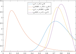
(a) Shapes of the three-parameter case

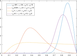
(b) Shapes of the four-parameter cases

Figure 2. The EPD for the three and four-parameter cases

This generalisation reduces to the two parameter extended power distribution if we set $\alpha_{2}=\alpha_{3}=\ldots=\alpha_{r-1}=0$ and to the $\text{Beta}(\alpha_{0},1)$, if we set $\alpha_{1}=\alpha_{2}=\alpha_{3}=\ldots=\alpha_{r-1}=0$. In a similar manner, setting $\alpha_{0}=1,\alpha_{1}=\alpha_{2}=\alpha_{3}=\ldots=\alpha_{r-1}=0$ gives the uniform distribution on $(0,1)$. For this generalisation, the cumulative distribution function is

$$F(t)=\exp\left\{\sum_{h=1}^{r}(-1)^{h-1}\alpha_{h-1}(\log t)^{h}\right\}$$ (3.12)

and we can simulate random variates using probability integral transform by finding the root of the polynomial

$$\sum_{h=1}^{r}(-1)^{h-1}\alpha_{h-1}(\log T)^{h}-\log U=0$$

which lies on $(0,1)$. This is more complicated than in the two parameter case, however, there are a number of available mathematical programs for calculating roots of a polynomial and we can easily utilise the roots function in MATLAB for this purpose. A similar scenario applies when calculating the median of the generalised distribution and we obtain the median ($M$) as a root of the polynomial

$$\sum_{h=1}^{r}(-1)^{h-1}\alpha_{h-1}(\log M)^{h}-\log 0.5=0.$$

Maximum likelihood estimators can be derived for the generalised extended power distribution by first obtaining the likelihood function and optimising using numerical methods. The log-likelihood function for the generalised density is

$$\ell(\alpha_{0},\alpha_{1},\ldots,\alpha_{r-1})= \sum_{i=1}^{n}\log\bigg{(}\sum_{h=1}^{r}\alpha_{h-1}(\log t_{i})^{h-1}h(-1)^{h-1}\bigg{)}-\sum_{i=1}^{n}\log t_{i}$$

$$+\sum_{h=1}^{r}(-1)^{h-1}\alpha_{h-1}\sum_{i=1}^{n}(\log t_{i})^{h}.$$

Differentiating the log-likelihood function with respect to $\alpha_{h-1}$, we get

$$\frac{\partial\ell}{\partial\alpha_{h-1}}=\sum_{i=1}^{n}\frac{(\log t_{i})^{h-1}h(-1)^{h-1}}{\sum_{h=1}^{r}\alpha_{h-1}(\log t_{i})^{h-1}h(-1)^{h-1}}+(-1)^{h-1}\sum_{i=1}^{n}(\log t_{i})^{h}$$ (3.13)

and second derivative

$$\frac{\partial^{2}\ell}{\partial\alpha_{h-1}\alpha_{k-1}}=\sum_{i=1}^{n}\frac{(\log t_{i})^{h+k-2}hk(-1)^{h+k-1}}{\bigg{(}\sum_{h=1}^{r}\alpha_{h-1}(\log t_{i})^{h-1}h(-1)^{h-1}\bigg{)}^{2}}.$$ (3.14)

3.6. Applications and Examples

In this subsection, we show examples where the extended power distribution is applicable. We also compare how well the extended power function fits actual data to how the Kumaraswamy distribution compares in performance. Finally, we will simulate data using the extended power distribution and try fitting the data with the Kumaraswamy distribution to see show cases where the extended power distribution has particular advantages over other bounded distributions. To fit the observed data, we will obtain maximum likelihood estimators for the parameters the distribution by maximising the log-likelihood functions for both the extended power distribution and the Kumaraswamy distribution. Table 2 shows the Akaike information criterion (AIC) of the fitted distributions in each application. The corrected AIC (AICc) and the Bayesian information criterion (BIC) which penalises more for extra parameters are given in tables 3 and 4 respectively. The MLE for the fitted distributions are detailed in table 5. In most of the examples, the extended power distribution performed better than the Kumaraswamy distribution (using AIC, AICc and BIC). The only exception is example 2, where the Kumaraswamy had the least BIC. The difference between this BIC and the BIC of the 3 parameter EPD is quite negligible.

Distribution	Kumaras.	2-Par EPD	3-Par EPD	4-Par EPD
Example 1	-88.6054	-70.4173	-91.9646	$\mathbf{-92.8209}$
Example 2	-82.7203	-67.5975	$\mathbf{-84.6515}$	-83.0609
Example 3	-153.3079	-170.5573	$\mathbf{-177.6280}$	-175.6280
Example 4	-82.4570	$\mathbf{-83.0053}$	-81.0053	-79.0053
Example 5	-669.9358	-719.9494	-814.5105	$\mathbf{-850.8778}$
Example 6	-795.4145	-965.8150	$\mathbf{-996.5056}$	$-994.5056$
Example 7		$\mathbf{-302.7052}$	-300.7052	-298.7052

Table 2. AIC for fitted distributions in examples 1-7, with the best fitting distribution in bold

Distribution	Kumaras.	2-Par EPD	3-Par EPD	4-Par EPD
Example 1	-88.4054	-70.2173	-91.5579	$\mathbf{-92.1313}$
Example 2	-82.5203	-67.3975	$\mathbf{-84.3447}$	-82.3712
Example 3	-153.1364	-170.3859	$\mathbf{-177.2802}$	-175.0398
Example 4	-82.2570	$\mathbf{-82.8053}$	-80.5985	-78.3156
Example 5	-669.9052	-719.9188	-814.4491	$\mathbf{-850.7753}$
Example 6	-795.4024	-965.8030	$\mathbf{-996.4815}$	$-994.4654$
Example 7		$\mathbf{-302.6230}$	-300.5396	-298.4274

Table 3. AICc for fitted distributions in examples 1-7, with the best fitting distribution in bold

Distribution	Kumaras.	2-Par EPD	3-Par EPD	4-Par EPD
Example 1	-84.3191	-66.1311	$\mathbf{-85.5352}$	-84.2484
Example 2	$\mathbf{-78.4340}$	-63.3113	-78.2221	-74.4883
Example 3	-148.7269	-165.9764	$\mathbf{-170.7566}$	-166.4662
Example 4	-78.1708	$\mathbf{-78.7190}$	-74.5759	-70.4327
Example 5	-661.9780	-711.9916	-802.5738	$\mathbf{-834.9623}$
Example 6	-785.5990	-955.9995	$\mathbf{-981.7823}$	$-974.8745$
Example 7		$\mathbf{-296.6973}$	-291.6933	-286.6894

Table 4. BIC for fitted distributions in examples 1-7, with the best fitting distribution in bold

Distribution	Kumaras.	2-Par EPD	3-Par EPD	4-Par EPD
Example 1	$\hat{\alpha}=4.51,\hat{\beta}=15.21$	$\hat{\alpha}_{0}=0.00,\hat{\alpha}_{1}=1.72$	$\hat{\alpha}_{0}=0.00,\hat{\alpha}_{1}=0.00,\hat{\alpha}_{2}=2.00$	$\hat{\alpha}_{0}=0.00,\alpha_{1}=0.00,\hat{\alpha}_{2}=0.73,\hat{\alpha}_{3}=1.39$
Example 2	$\hat{\alpha}=4.31,\hat{\beta}=13.06$	$\hat{\alpha}_{0}=0.00,\hat{\alpha}_{1}=1.68$	$\hat{\alpha}_{0}=0.00,\hat{\alpha}_{1}=0.00,\hat{\alpha}_{2}=1.90$	$\hat{\alpha}_{0}=0.00,\alpha_{1}=0.00,\hat{\alpha}_{2}=1.45,\hat{\alpha}_{3}=0.47$
Example 3	$\hat{\alpha}=0.66,\hat{\beta}=3.44$	$\hat{\alpha}_{0}=0.01,\hat{\alpha}_{1}=0.10$	$\hat{\alpha}_{0}=0.04,\hat{\alpha}_{1}=0.00,\hat{\alpha}_{2}=0.02$	$\hat{\alpha}_{0}=0.04,\hat{\alpha}_{1}=0.00,\hat{\alpha}_{2}=0.02,\hat{\alpha}_{3}=0.00$
Example 4	$\hat{\alpha}=5.85,\hat{\beta}=3.03$	$\hat{\alpha}_{0}=0.25,\hat{\alpha}_{1}=7.03$	$\hat{\alpha}_{0}=0.25,\hat{\alpha}_{1}=7.03,\hat{\alpha}_{2}=0.00$	$\hat{\alpha}_{0}=0.25,\hat{\alpha}_{1}=7.03,\hat{\alpha}_{2}=0.00,\hat{\alpha}_{3}=0.00$
Example 5	$\hat{\alpha}=1.00,\hat{\beta}=5.28$	$\hat{\alpha}_{0}=0.00,\hat{\alpha}_{1}=0.17$	$\hat{\alpha}_{0}=0.03,\hat{\alpha}_{1}=0.00,\hat{\alpha}_{2}=0.06$	$\hat{\alpha}_{0}=0.07,\hat{\alpha}_{1}=0.00,\hat{\alpha}_{2}=0.00,\hat{\alpha}_{3}=0.02$
Example 6	$\hat{\alpha}=3.58,\hat{\beta}=2.05$	$\hat{\alpha}_{0}=0.51,\hat{\alpha}_{1}=3.38$	$\hat{\alpha}_{0}=0.90,\hat{\alpha}_{1}=0.62,\hat{\alpha}_{2}=3.22$	$\hat{\alpha}_{0}=0.90,\hat{\alpha}_{1}=0.62,\hat{\alpha}_{2}=3.22,\hat{\alpha}_{3}=0.00$
Example 7		$\hat{\alpha}_{0}=6.53,\hat{\alpha}_{1}=0.00$	$\hat{\alpha}_{0}=6.53,\hat{\alpha}_{1}=0.00,\hat{\alpha}_{2}=0.00$	$\hat{\alpha}_{0}=6.53,\hat{\alpha}_{1}=0.00,\hat{\alpha}_{2}=0.00,\hat{\alpha}_{3}=0.00$

Table 5. MLE for fitted distributions in examples 1-7

3.6.1. Example 1

In this example, we explore data on US senate voting patterns from 1953 to 2015. The observed data are proportion of party unity votes in which a majority of voting Democrats opposed a majority of voting Republicans. The data is taken from the Brookings Institution (Brookings (2017)) and is available for free. A histogram of the actual data and its empirical cumulative distribution along with fitted density and distribution functions are given in figure 3. From the fitted distributions, we see that the four-parameter extended power distribution best fits the actual data.

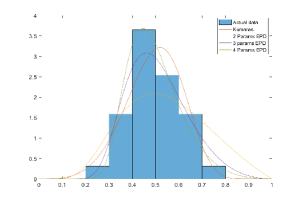
(a) Density functions fitted to histogram

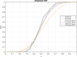
(b) Fitting cdfs to the empirical cdf

Figure 3. Fitting proportion of US Senate party unity votes using the Kumaraswamy and extended power distributions

3.6.2. Example 2

This second data explores proportion of unity votes in the US House of Representatives from 1953 to 2015. The data is also from Brookings (2017). A histogram (and empirical cumulative distribution) of the actual data and fitted distributions using MLE are shown in figure 4. In this case, the three-parameter and four-parameter extended power distribution give the best fit, with the four-parameter case having a slightly higher peak. From the cumulative distribution plot, we see that at the lower tail, the three and four-parameter extended power distribution function best fits the empirical distribution function.

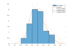
(a) Density functions fitted to histogram

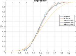
(b) Fitting cdfs to the empirical cdf

Figure 4. Fitting proportion of US House of Representatives party unity votes using the Kumaraswamy and extended power distributions

3.6.3. Example 3

This data which is taken from Jodrá and Jiménez-Gamero (2016) and is a measure of a firm’s risk management cost effectiveness given as a proportion. This data has been used in Jodrá and Jiménez-Gamero (2016) for regression modelling using the beta and log-Lindley distributions. The extended power distribution gives the best fit for this data and even has smaller AIC than that obtained for the log-Lindley distribution (Gómez-Déniz et al. (2014)) which is $-149.2083$.

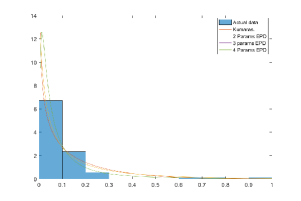
(a) Density functions fitted to histogram

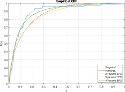
(b) Fitting cdfs to the empirical cdf

Figure 5. Fitting risk management cost effectiveness using the Kumaraswamy and extended power distributions

3.6.4. Example 4

This example involves proportion of presidential bill victories in the US Senate from President Einsenhower in 1953 to President Obama in 2015 (obtained from Brookings (2017)). The fitted distributions are shown in figure 6. In this case, the two-parameter extended power distribution seems to give the best fit.

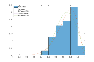
(a) Density functions fitted to histogram

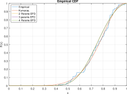
(b) Fitting cdfs to the empirical cdf

Figure 6. Fitting proportion of US senators of who support presidential bills using the Kumaraswamy and extended power distributions

3.6.5. Example 5

This example is taken from the 2011 census data on the proportion of minority ethnic groups across different local authorities in England and Wales. The data is obtained from the Office of National Statistics 2011 census (ONS (2011)) and the minorities include groups such as white Irish, white and black Caribbean, Arabian, etc. The extended power distribution has the best fit for this example.

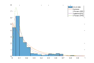
(a) Density functions fitted to histogram

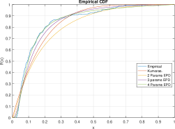
(b) Fitting cdfs to the empirical cdf

Figure 7. Fitting proportion of ethnic minorities in different local authorities in England and Wales using the Kumaraswamy and extended power distributions

3.6.6. Example 6

In this example, we simulate data ($n=1000$) from the three-parameter extended power distribution with parameters $\alpha_{0}=1$, $\alpha_{1}=0.001$ and $\alpha_{4}=4$. We then fit the simulated data using the Kumaraswamy distribution. From figure 8, we see that the the Kumaraswamy distribution fails to properly fit the data as values of the random variable approaches 1.

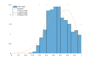
(a) Density functions fitted to histogram

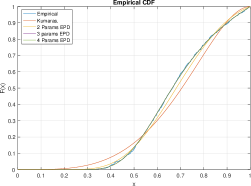
(b) Fitting cdfs to the empirical cdf

Figure 8. Fitting a Kumaraswamy distribution and extended power distribution to data simulated from the three-parameter extended power distribution

3.6.7. Example 7

This example, obtained from the UNICEF website (UNICEF (2015)) contains the proportion of literate youths in 149 different countries (updated in October, 2015). Figure 9 show a plot of the actual data as well as the maximum likelihood fits. In this example, the Kumaraswamy distribution is not applicable, because some countries have youth literacy of $100\%$ (that is proportion is 1), however, the Kumaraswamy distribution has density converging to 0 (for $\beta>1$) and to $\infty$ (for $\beta<1$) when $t$ is exactly 1, making the log-likelihood function undefined at $t=1$ and the MLE cannot be computed. For this example, the two-parameter extended power distribution has the smallest AIC values, hence gives the best fit.

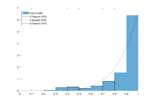
(a) Density functions fitted to histogram

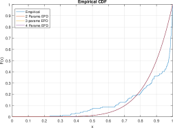
(b) Fitting cdfs to the empirical cdf

Figure 9. Fitting youths literacy rates in 149 different countries using the Kumaraswamy and extended power distributions

4. Complementary Distribution

The complementary distribution for the beta distribution has been defined in Jones (2002) and are obtained by considering the quantile functions and as the cumulative distribution function of a probability distribution on $(0,1)$. This same procedure can be considered for other bounded distribution on $(0,1)$ to get a new bounded distribution. In the complementary beta distribution, the form of density function and moments involve the use of special function as given in Jones (2002). However, for the complementary Kumarawamy distribution (Jones (2009)), even though the density function can be written in a nice form, there is nothing new to be seen in its form because it is equivalent to $g(1-t,\frac{1}{\beta},\frac{1}{\alpha})$, where $g\sim\text{Kumaraswamy}(t,\alpha,\beta)$.

In this section, we will define the complementary extended power distribution, its properties such as moments, quantiles and parameter estimation. The density function of the complementary extended power distribution is obtained by taking the first derivative of the quantile function. The quantile function is given as

$$Q(t)=F^{-1}(t)=\exp\left\{\frac{-\alpha_{0}+(\alpha_{0}^{2}-4\alpha_{1}\log(t))^{1/2}}{-2\alpha_{1}}\right\},$$

hence the density function of the proposed complementary extended power distribution is

$$q(t)=\frac{1}{t}(\alpha_{0}^{2}-4\alpha_{1}\log t)^{-1/2}\exp\left\{\frac{-\alpha_{0}+(\alpha_{0}^{2}-4\alpha_{1}\log(t))^{1/2}}{-2\alpha_{1}}\right\}.$$ (4.1)

An interesting properties of this distribution on first sight is that both its density function and distribution are available in a simple closed form without the need for any special function. Secondly, it has a form which is not exactly similar to the extended power distribution, implying some new information may be gained.

An interesting special case of the complementary extended power distribution is obtained by setting $\alpha_{1}=0$. Simply replacing $\alpha_{1}=0$ in equation 4.1, will make the exponent indeterminate. To deal with this problem, we use binomial expansion on $(\alpha_{0}^{2}-4\alpha_{1}\log(t))^{1/2}$, hence the density function becomes

$$q(t)=\frac{1}{t}(\alpha_{0}^{2}-4\alpha_{1}\log t)^{-1/2}\exp\left\{\frac{1}{\alpha_{0}}\log t+\frac{\alpha_{1}(\log t)^{2}}{\alpha_{0}^{3}}+\frac{2\alpha_{1}^{2}(\log t)^{3}}{\alpha_{0}^{5}}+\ldots\right\},\quad t\in(0,1)$$

and setting $\alpha_{1}=0$ gives

$$q(t)=\frac{1}{\alpha_{0}}t^{\frac{1}{\alpha_{0}}-1}$$

which corresponds to a $\text{Beta}(\frac{1}{\alpha_{0}},1)$ or a $\text{Kumaraswamy}(\frac{1}{\alpha_{0}},1)$. Like in the extended power distribution considered earlier, fixing $\alpha_{0}=1$ and $\alpha_{1}=0$, $q(t)$ reduces to the density for a uniform distribution on $(0,1)$. If T is a random variable from the two-parameter complementary extended power distribution, with $\alpha_{1}=0$, then the random variable $V=-\log T$ follows an exponential distribution with density function

$$f(v)=\frac{1}{\alpha_{0}}\exp\{-\frac{v}{\alpha_{0}}\}.$$

Generating random variates from the complementary extended power distribution is straightforward using the probability integral transform. If $U\sim U(0,1)$, then we simulate random variables T using,

$$T=\exp\left\{\alpha_{0}\log U-\alpha_{1}(\log U)^{2}\right\}.$$ (4.2)

4.1. Moments, Quantiles and Mode

In this section, we will give formulas for the moments, quantiles and mode of the complementary extended power distribution. We will begin by giving a formula for the $kth$ moment of the complementary extended power distribution. This makes it easier to calculate quantities such as the variance, skewness and kurtosis.

Theorem 4.1.

The $kth$ moment of the complementary extended power distribution is

$$E(T^{k})=\frac{1}{2}\sqrt{\frac{\pi}{\alpha_{1}k}}\exp\left\{\frac{(4\alpha_{0}\alpha_{1}k+4\alpha_{1})^{2}}{64\alpha_{1}^{3}k}\right\}\text{erfc}\bigg{(}\frac{4\alpha_{0}\alpha_{1}k+4\alpha_{1}}{8\alpha_{1}^{3/2}k^{1/2}}\bigg{)}.$$ (4.3)

Proof.

$$E(T^{k})=\int_{0}^{1}t^{k-1}(\alpha_{0}^{2}-4\alpha_{1}\log t)^{-1/2}\exp\left\{\frac{-\alpha_{0}+(\alpha_{0}^{2}-4\alpha_{1}\log(t))^{1/2}}{-2\alpha_{1}}\right\}dt.$$

If we define $u=\frac{-\alpha_{0}+(\alpha_{0}^{2}-4\alpha_{1}\log(t))^{1/2}}{-2\alpha_{1}}$, we have

$$E(T^{k})=\exp\left\{\alpha_{1}k\bigg{(}\ \frac{4\alpha_{0}\alpha_{1}k+4\alpha_{1}}{8\alpha_{1}^{2}k}\bigg{)}^{2}\right\}\int_{-\infty}^{0}\exp\left\{-\alpha_{1}k\bigg{[}u-\bigg{(}\ \frac{4\alpha_{0}\alpha_{1}k+4\alpha_{1}}{8\alpha_{1}^{2}k}\bigg{)}\bigg{]}^{2}\right\}du.$$

Simplifying further, we have the final result as

$$E(T^{k})=\frac{1}{2}\sqrt{\frac{\pi}{\alpha_{1}k}}\exp\left\{\frac{(4\alpha_{0}\alpha_{1}k+4\alpha_{1})^{2}}{64\alpha_{1}^{3}k}\right\}\text{erfc}\bigg{(}\frac{4\alpha_{0}\alpha_{1}k+4\alpha_{1}}{8\alpha_{1}^{3/2}k^{1/2}}\bigg{)}.$$

∎

With this result, we have $E(T)$ and $Var(T)$ as

$$E(T)= \frac{1}{2}\sqrt{\frac{\pi}{\alpha_{1}}}\exp\left\{\frac{(4\alpha_{0}\alpha_{1}+4\alpha_{1})^{2}}{64\alpha_{1}^{3}}\right\}\text{erfc}\bigg{(}\frac{4\alpha_{0}\alpha_{1}+4\alpha_{1}}{8\alpha_{1}^{3/2}}\bigg{)}$$

$$Var(T)= \frac{1}{2}\sqrt{\frac{\pi}{2\alpha_{1}}}\exp\left\{\frac{(8\alpha_{0}\alpha_{1}+4\alpha_{1})^{2}}{128\alpha_{1}^{3}}\right\}\text{erfc}\bigg{(}\frac{8\alpha_{0}\alpha_{1}+4\alpha_{1}}{(2^{7/3}\alpha_{1})^{3/2}}\bigg{)}$$

$$-\frac{1}{4}\frac{\pi}{\alpha_{1}}\exp\left\{\frac{(4\alpha_{0}\alpha_{1}+4\alpha_{1})^{2}}{32\alpha_{1}^{3}}\right\}\left\{\text{erfc}\bigg{(}\frac{4\alpha_{0}\alpha_{1}+4\alpha_{1}}{8\alpha_{1}^{3/2}}\bigg{)}\right\}^{2}.$$

The median for the complementary extended power distribution is

$$Q_{0.5}=\exp\left\{\alpha_{0}\log(0.5)-\alpha_{1}(\log(0.5))^{2}\right\}.$$

and the mode is obtainable in a closed form by calculating the first derivative of $q(t)$ and equating to zero. Hence, we can calculate the mode by solving the cubic equation

$$A_{0}+A_{1}\log t+A_{2}(\log t)^{2}+A_{3}(\log t)^{3}=0$$ (4.4)

where

$$A_{0} = \alpha_{0}^{2}-4\alpha_{0}^{4}\alpha_{1}+4\alpha_{0}^{6}\alpha_{1}^{2}-1$$

$$A_{1} = -48\alpha_{0}^{4}\alpha_{1}^{3}-4\alpha_{1}$$

$$A_{2} = 192\alpha_{0}^{2}\alpha_{1}^{4}-64\alpha_{1}^{3}$$

$$A_{3} = -256\alpha_{1}^{5}.$$

4.2. Maximum Likelihood Estimation

The log-likelihood function of the complementary extended power distribution is

$$\ell(\alpha_{0},\alpha_{1})=\sum_{i=1}^{n}\log(\alpha_{0}^{2}-4\alpha_{1}\log t_{i})^{-1/2}-\sum_{i=1}^{n}\log t_{i}+\frac{\alpha_{0}n}{2\alpha_{1}}-\frac{1}{2\alpha_{1}}\sum_{i=1}^{n}(\alpha_{0}^{2}-4\alpha_{1}\log t_{i})^{1/2}$$ (4.5)

and we have the following system of equations by differential the log-likelihood

$$\frac{\partial\ell(\alpha_{0},\alpha_{1})}{\partial\alpha_{0}} = -\alpha_{0}\sum_{i=1}^{n}(\alpha_{0}^{2}-4\alpha_{1}\log t_{i})^{-1}+\frac{n}{2\alpha_{1}}-\frac{\alpha_{0}}{2\alpha_{1}}\sum_{i=1}^{n}(\alpha_{0}^{2}-4\alpha_{1}\log t_{i})^{-1/2}=0$$

$$\frac{\partial\ell(\alpha_{0},\alpha_{1})}{\partial\alpha_{0}} = 2\sum_{i=1}^{n}\log t_{i}(\alpha_{0}^{2}-4\alpha_{1}\log t_{i})^{-1}-\frac{\alpha_{0}n}{2\alpha_{1}^{2}}-\frac{\alpha_{1}^{-3}}{2}\sum_{i=1}^{n}(\alpha_{0}^{2}-4\alpha_{1}\log t_{i})^{-1/2}=0.$$

Like in the extended power function, we can apply non-linear optimisation to estimate the unknown parameters.

5. Conclusion

A bounded probability distribution motivated by warping functions in functional data analysis is proposed. We have explored properties of the extended power distribution (EPD), such as moments and applications. We have given special cases of the distribution which are related to the Raleigh distribution, exponential distribution, beta distribution and linear hazard rate distribution (Bain (1974)). In this work, closed forms for the mode, median and other quantiles were given. An important property of this distribution over the beta distribution is that we have its cumulative distribution function and quantile function available in simple mathematical forms which makes it easy to simulate using the probability integral transform.

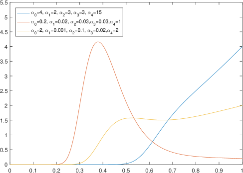
Figure 10. Plots of the 5-parameter extended power distribution for different parameter values showing some extra flexibilities

We note that the Kumaraswamy distribution and extended power distribution have some interesting properties in common, such as a closed form for their cumulative distribution and quantile functions. However, unlike Kumaraswamy distribution, the extended power distribution is easily extendable from a two-parameter to a muilti-parameter distribution. This multi-parameter extension comes with added flexibility as we have seen in some applications in this work. In figure 10 for example, we show a five-parameter case of the extended power distribution with different parameter choices. Another advantage of the extended power distribution is that as $t$ nears $1$, the density approaches the parameter $\alpha_{0}$, while the density function of the Kumaraswamy distribution (and the beta distribution) approaches $0$ or $\infty$, as $t$ approaches $1$. This is useful in applications where there is a high proportion of observed values closer to the upper bound.

The generalisation of the extended power distribution makes computing moments more complicated and would involve numerical integration. However, simulations using the probability integral transform are less complicated and would involve finding the roots of a polynomial (same applies to the median). We can also estimate the parameters of the generalised extended power distribution numerically, using maximum likelihood.

Like in Jones (2002), we have proposed a complementary extended power distribution, which is the distribution derived from the quantile of the extended power distribution. We have shown that this distribution is linked to the beta distribution and the exponential distribution with inverted parameters. Simulation from this distribution, are easy using the probability integral transform because of the closed form of the cumulative density of the extended power distribution. However, the mode of the complementary extended power distribution is not available in closed form, but can the calculated as the solution to a cubic equation.

Figure 11. Fitting distributions to skewed data with high peak

We note that for skewed data (either left or right skewed) with very high peaks, the Kumaraswamy distribution gives a better fit than both the beta distribution and extended power distribution. This is seen in figure 11, for data containing information on employment rates in different counties in the US (BLS (2017)). The Kumaraswamy distribution has a higher peak than the two, three and four-parameter extended power distribution.

In the future, more applications peculiar to the extended power distribution needs to be explored. It will also be interesting to consider a new family of distributions by combining the extended power distribution and its complementary distribution. Just like the beta regression models are used for modelling bounded responses, we believe the extended power distribution can be alternative to the beta distribution. Programs for calculating different quantities related to extended power distribution are available in MATLAB.

References

- Akinsete et al. [2008] Alfred Akinsete, Felix Famoye, and Carl Lee. The beta-pareto distribution. Statistics, 42(6):547–563, 2008.
- Bain [1974] Lee J Bain. Analysis for the linear failure-rate life-testing distribution. Technometrics, 16(4):551–559, 1974.
- Barreto-Souza et al. [2010] Wagner Barreto-Souza, Alessandro HS Santos, and Gauss M Cordeiro. The beta generalized exponential distribution. Journal of Statistical Computation and Simulation, 80(2):159–172, 2010.
- BLS [2017] BLS. Local area unemployment statistics. https://www.bls.gov/web/metro/laucntycur14.txt, 2017. Accessed: 2017-09-30.
- Brookings [2017] Brookings. Vital statistics on congress. https://www.brookings.edu/multi-chapter-report/vital-statistics-on-congress/, 2017. Accessed: 2017-09-15.
- Cordeiro and de Castro [2011] Gauss M Cordeiro and Mario de Castro. A new family of generalized distributions. Journal of statistical computation and simulation, 81(7):883–898, 2011.
- Cordeiro et al. [2010] Gauss M Cordeiro, Edwin MM Ortega, and Saralees Nadarajah. The kumaraswamy weibull distribution with application to failure data. Journal of the Franklin Institute, 347(8):1399–1429, 2010.
- Cordeiro et al. [2012] Gauss M Cordeiro, Saralees Nadarajah, and Edwin MM Ortega. The kumaraswamy gumbel distribution. Statistical Methods & Applications, 21(2):139–168, 2012.
- de Pascoa et al. [2011] Marcelino AR de Pascoa, Edwin MM Ortega, and Gauss M Cordeiro. The kumaraswamy generalized gamma distribution with application in survival analysis. Statistical methodology, 8(5):411–433, 2011.
- Eugene et al. [2002] Nicholas Eugene, Carl Lee, and Felix Famoye. Beta-normal distribution and its applications. Communications in Statistics-Theory and methods, 31(4):497–512, 2002.
- Ferrari and Cribari-Neto [2004] Silvia Ferrari and Francisco Cribari-Neto. Beta regression for modelling rates and proportions. Journal of Applied Statistics, 31(7):799–815, 2004.
- Gómez-Déniz et al. [2014] Emilio Gómez-Déniz, Miguel A Sordo, and Enrique Calderín-Ojeda. The log–lindley distribution as an alternative to the beta regression model with applications in insurance. Insurance: Mathematics and Economics, 54:49–57, 2014.
- Gordy et al. [1998] Michael B Gordy et al. A generalization of generalized beta distributions. Division of Research and Statistics, Division of Monetary Affairs, Federal Reserve Board, 1998.
- Jafari and Mahmoudi [2012] Ali Akbar Jafari and Eisa Mahmoudi. Beta-linear failure rate distribution and its applications. arXiv preprint arXiv:1212.5615, 2012.
- Jodrá and Jiménez-Gamero [2016] P Jodrá and MD Jiménez-Gamero. A note on the log-lindley distribution. Insurance: Mathematics and Economics, 71:189–194, 2016.
- Jones [2002] MC Jones. The complementary beta distribution. Journal of Statistical Planning and Inference, 104(2):329–337, 2002.
- Jones [2004] MC Jones. Families of distributions arising from distributions of order statistics. Test, 13(1):1–43, 2004.
- Jones [2009] MC Jones. Kumaraswamy’s distribution: A beta-type distribution with some tractability advantages. Statistical Methodology, 6(1):70–81, 2009.
- Kumaraswamy [1980] Ponnambalam Kumaraswamy. A generalized probability density function for double-bounded random processes. Journal of Hydrology, 46(1-2):79–88, 1980.
- McDonald and Xu [1995] James B McDonald and Yexiao J Xu. A generalization of the beta distribution with applications. Journal of Econometrics, 66(1):133–152, 1995.
- Nadarajah and Kotz [2003] Saralees Nadarajah and Samuel Kotz. A generalized beta distribution ii. InterStat, 2003.
- Nadarajah and Kotz [2004] Saralees Nadarajah and Samuel Kotz. The beta gumbel distribution. Mathematical Problems in Engineering, 2004(4):323–332, 2004.
- Nadarajah and Kotz [2006] Saralees Nadarajah and Samuel Kotz. The beta exponential distribution. Reliability engineering & system safety, 91(6):689–697, 2006.
- ONS [2011] ONS. People, population and community. https://www.ons.gov.uk/peoplepopulationandcommunity/culturalidentity/ethnicity/articles/ethnicityandnationalidentityinenglandandwales/2012-12-11, 2011. Accessed: 2017-09-20.
- Sarhan and Kundu [2009] Ammar M Sarhan and Debasis Kundu. Generalized linear failure rate distribution. Communications in Statistics—Theory and Methods, 38(5):642–660, 2009.
- Sen [2006] Ananda Sen. Linear hazard rate distribution. Encyclopedia of Statistical Sciences, 2006.
- Sen and Bhattacharyya [1995] Ananda Sen and Gouri K Bhattacharyya. Inference procedures for the linear failure rate model. Journal of Statistical Planning and Inference, 46(1):59–76, 1995.
- UNICEF [2015] UNICEF. Education and literacy. https://data.unicef.org/topic/education/overview/, 2015. Accessed: 2017-09-30.