About simple variational splines
from the Hamiltonian viewpoint

Abstract

In this paper, we study simple splines on a Riemannian manifold $Q$ from the point of view of the Pontryagin maximum principle (PMP) in optimal control theory. The control problem consists in finding smooth curves matching two given tangent vectors with the control being the curve’s acceleration, while minimizing a given cost functional. We focus on cubic splines (quadratic cost function) and on time-minimal splines (constant cost function) under bounded acceleration. We present a general strategy to solve for the optimal hamiltonian within the PMP framework based on splitting the variables by means of a linear connection. We write down the corresponding hamiltonian equations in intrinsic form and study the corresponding hamiltonian dynamics in the case $Q$ is the $2$-sphere. We also elaborate on possible applications, including landmark cometrics in computational anatomy.

2010 MSC: 53D20, 65D07; 49J15, 70H06

keywords: Riemannian splines, Computational anatomy,
                      Geometric control, Reduction, Reconstruction

Paula Balseiro

Departamento de Matemática Aplicada, Universidade Federal Fluminense

Rua Mário Santos Braga, S/N, Campus do Valonguinho

24020-140, Niterói, RJ, Brazil

pbalseiro@vm.uff.br

Teresinha J. Stuchi

Departamento de Física Matemática, Universidade Federal do Rio de Janeiro

Centro de Tecnologia - Bloco A - Cidade Universitária - Ilha do Fundão

21941-972 Rio de Janeiro - RJ - Brazil

emailtstuchi@if.ufrj.br

Alejandro Cabrera

Departamento de Matemática Aplicada, Universidade Federal do Rio de Janeiro

Centro de Tecnologia - Bloco C - Cidade Universitária - Ilha do Fundão

21941-909 Rio de Janeiro - RJ - Brazil

acabrera@labma.ufrj.br

Jair Koiller

Instituto Nacional de Metrologia, Qualidade e Tecnologia

Divisão de Metrologia em Dinâmica de Fluidos

25250-020, Xerém, Duque de Caxias - RJ - Brazil

jairkoiller@gmail.com

1 Introduction

Cubic Riemannian splines and their higher order extensions have been instrumental for interpolation and statistics on manifolds. The bibliography is vast, see e.g. [85], [50], [49], [26], [46], [47], [77], [95], [43]. In this note we consider only the simplest case, namely, of splines having the tangent bundle as state space, the acceleration vector being the control. We remark that a tangent vector gives a minimal model for a short process. For instance, the rendezvous problem in robotics and in space science ([45], [91], [70]) consists of planning a path with prescribed initial and end tangent vectors. For instance, to achieve a smooth docking of a service spacecraft to the International Space Station.

In computational anatomy [101] splines are useful for longitudinal medical studies [42], [89],[90], [40], combined with adaptive machine learning techniques, see e.g. [76], [97]. However, the idea of comparing two short physiological processes seems not much explored as yet. This question is important in embryology, where it is called morphokinetics [36].

There is a potential use of simple splines also in sport science, computer animation, recognition, and video/movies repair, see [15] and references therein.

Let us now present our general framework, which belongs to the class of so-called mechanical control problems. These were first studied via Geometric Mechanics in Andrew Lewis thesis [66], consolidating earlier work by several authors, specially R. Brocket, J. Baillieul, A. Van der Schaft, P. Crouch and A. Bloch. The standard reference is the book by Bullo and Lewis [24], where the Lagrangian viewpoint is mostly used.

One considers a configuration space $Q$ endowed with a Riemannian (kinetic energy) metric $g$. The organism or device under study is controlled by forces that produce an acceleration $u$, taken here as the control variable. If $\nabla$ denotes the Levi-Civita connection, the state equation on the tangent bundle $TQ$ is

$$\nabla_{\dot{q}}\dot{q}=u\,.$$ (1)

The aim is to connect two tangent vectors (or ’short processes’) $v_{q_{0}},w_{q_{1}}\in TQ$ minimizing a cost functional. In this paper, we focus on the following two special cases which have received special attention.

Cubic splines on a Riemannian manifold, which were introduced around 1990 ([81, 34]), correspond to minimizing the cost functional:

$$\int_{0}^{T}\,\frac{\beta}{2}\,|u|^{2}\,dt,$$ (2)

with prescribed time $T$. Cubic splines have been extensively used in computational anatomy.

The other special case is the time minimal problem under bounded acceleration. It consists in connecting two vectors in minimum time, under the restriction

$$|u|\leq A\,,\,\,{\rm where}\,A\,{\rm is}\,{\rm a}\,{\rm prescribed}\,{\rm bound.}$$ (3)

There is no accessibility issue: for any arbitrarily small bound $\epsilon$ on $|u|$, under mild hypothesis on $Q$ it is possible to concatenate any two tangent vectors by a smooth curve with non vanishing velocity and acceleration norm $\leq\epsilon$ [99]. The time minimal-bounded acceleration problem is in general (though not always) equivalent to the $L^{\infty}$ control problem considered recently by Noakes and Kaya [58], [80], where they ask for a trajectory that minimizes the sup of the norms of the accelerations, with fixed transition time.

From now on we shall refer to cubic splines also as $L^{2}$-splines, due to the form of the underlying cost functional (2), and to time minimal-bounded acceleration splines as $L^{\infty}$-splines, due to the previous discussion.

Via Pontryagin’s maximum principle, every cost functional associated to (1) yields a Hamiltonian system in $\,\,T^{*}(TQ)$. In this paper, we study the resulting Hamiltonian systems in detail.

1.1 Motivations

Splines in $S^{m}$.

According to Lyle Noakes, “the problem of interpolating and approximating spherical data in the m-dimensional manifold $S^{m}$ is much more widespread than might at first be thought” [78]. Indeed, see [98], [41], [18], [37] for information on spherical statistics.

In order to match two infinitesimal processes on $TS^{m}$ with simple variational splines, it seems to us that it is sufficient to understand the cases $m=1,2,3$. This is due to homogeneity under $SO(m+1)$ action: any two tangent vectors $v_{q_{1}},w_{q_{2}}$ on ‘big’ $TS^{N}$ are actually tangent to a isometrically imbedded $S^{m}$ with $m\leq 3$.

(For the analogous problem on $\mathbb{R}^{N}$, $q_{1}$ can be the origin, $v_{1}$, $q_{1}-q_{2}$ and $v_{2}$ define at most a three dimensional subspace.)

We have collected a number of references on cubic splines on $S^{2}$. Somewhat surprisingly, as far as we know, the reduction of the $SO(3)$-symmetry of $T^{*}(TS^{2})$ by Hamiltonian methods was still awaiting. We present here a reduction procedure, but we must confess that it works well only outside the zero section.

Splines in Diff

The systems studied in this paper can be taken as finite-dimensional toy models for the following infinite-dimensional one. Following the notations of [51], let $\mathcal{D}$ a domain in $\mathbb{R}^{d}$ and ${\rm Diff}(\mathcal{D}),\,\mathcal{X}$ respectively the group of diffeomorphisms $\phi$ and vector fields ${\bf u}(x)$ with appropriate boundary conditions. The idea is to consider control systems as in (1) but now on the infinite dimensional $Q={\rm Diff}$. Upon right translations, one has $T{\rm Diff}={\rm Diff}\times\mathcal{X}$, $T^{*}{\rm Diff}={\rm Diff}\times\mathcal{X}^{*}$. With due care to functional analysis, $\mathcal{X}^{*}$ is the space of momentum densities $\bf{m}$, with $m=\bf{m}\cdot{\bf dx}\otimes dV$. Consider a Sobolev metric on ${\rm Diff}$ ([22], [48], [72], [12], [13], [16], [17], [11]). One can write

$$L=\frac{1}{2}\,\int\,{\bf u}(x)\cdot{\bf m}(x)dV\qquad\mbox{and}\qquad{\bf u}(x)=\int\,G(x,y)\,{\bf m}(y)\,dV(y),$$ (4)

where $G(x,y)$ is the Green function for the inverse of the linear partial differential operator that yields ${\bf m}$ when applied to ${\bf u}$.

EPDiff (geodesics on Diff), the celebrated Euler-Poincaré partial differential equation in terms of the momentum density is given by

$$\frac{\partial}{\partial t}\,\bf{m}+\bf{u}\cdot\nabla\bf{m}+(\nabla\bf{u})^{T}\cdot\bf{m}+\bf{m}({\rm div}\,\bf{u})=0\,\,\,\,\,\,{\rm(EPDiff)},$$ (5)

and comes from a noble tradition going back to Arnold’s interpretation of Euler’s incompressible fluid equations as geodesics in the infinite dimensional Lie group of volume preserving diffeomorphisms [75]. One of the striking facts is that often the solutions of EPDiff tend to concentrate on pulson submanifolds

$${\bf m}(x,t)=\sum_{i}^{N}\,\int\,{\bf P}_{i}(s,t)\,\delta(x-{\bf Q}_{i}(s,t)).$$

In turn, from singular momentum solutions one recovers the vector fields via

$${\bf u}(x,t)=\sum_{i}^{N}\,\int\,{\bf P}_{i}(s,t)\,G(x,{\bf Q}_{i}(s,t))\,ds\,\,.$$ (6)

Mario Michelli [71, 72] implemented geodesic equations for landmarks. His formulae for for Christoffel symbols and curvatures coefficients in terms of cometrics, can be used to implement a code for landmark splines using our methodology. In the infinite dimensional case cubic splines have only recently been considered [89], [90]. We will discuss the open problem of relating landmark splines to the infinite dimensional problem in the final section.

1.2 Contents of the paper

In section 2, we study the control problem associated to the state equation (1) from the point of view of Pontryagin maximum principle (PMP). The main theoretical results of the paper are intrinsic formulas for the optimal hamiltonian and the resulting hamiltonian equations (Propositions 1 and 2). The key idea is to use split variables for $T^{*}(TQ)$ coming from taking horizontal and vertical components w.r.t. the underlying linear connection on $TQ$. A dual splitting of $T(TQ)$ was already explored by Lewis and Murray and is presented in full details in Bullo and Lewis [25]. In [7] we generalize the construction to $T^{*}A$, for $A\to Q$ a vector bundle with a connection.

In split variables, the symplectic form is no longer canonical (it contains curvature terms, Proposition 1) but the parametric hamiltonian appearing from the PMP has a simple form. We can then find the optimal hamiltonian for cubic and time-minimal splines easily and derive the corresponding hamiltonian equations in intrinsic form (Proposition 2). We show that, in the particular case $Q=S^{n}$ a $n$-sphere, we recover the higher dimensional case analogue to the hamiltonian system for cubic splines derived by Crouch and Leite [34, 33] for $S^{2}$.

In section 3, we study dynamical aspects of the resulting hamiltonian equations on $T^{*}(TQ)$ in the particular case of cubic splines on $Q=S^{2}$. Our main technical tool in this study is reduction by the natural rotation symmetry. The reduced system has two degrees of freedom. Two known families of solutions for cubic splines on $S^{2}$ are reinterpreted. They correspond to equilibria and partial equilibria of the reduced system. i) “Figure eights” formed by two kissing circles with geodesic curvature $\kappa_{g}=1$, run uniformly in time. They correspond to unstable, loxodromic, fixed points of the reduced Hamiltonian. ii) Equators, run cubically on time, correspond to “partially fixed” points of the reduced system. Moreover, in section 3.3 we discuss some numerical simulations. Poincaré sections indicate that the reduced system is non-integrable, but has regions rich of invariant tori. In section 3.4, we discuss the limitations of the reduction procedure (coming from the rotation action not being free at zero tangent vectors) and provide the explicit relation to the general split variables approach.

Section 4 contains some further comments and presents suggestions for further research. In particular, since it is well known that landmark geodesics lift to geodesic solutions on the full ${\rm Diff}$ [71], [23], we pose the question if landmark splines can be lifted to splines on ${\rm Diff}$.

In appendix A, we present a simple Fortran program used for the reconstruction of trajectories in $S^{2}$. It uses the Runge-Kutta-Fehlberg routine RK78 ([39]) which is of standard use in Celestial Mechanics [5]. In appendix B, we discuss how to interpret the controls entering the state equation (1) in terms of curvatures of the underlying curve, in the particular case $Q=\Sigma\subset\mathbb{R}^{3}$ is a convex surface. These results are applied in section 3.

2 Optimal control on $TQ$ as state space

As mentioned in the introduction, our main object of study will be the following optimal control problem. The state space is $TQ$, where $(Q,g)$ is a Riemannian manifold, and the control is represented by a (force or acceleration) vector field $u\in\mathcal{X}(Q)$. The state equations (1) can be written in first-order form as

$$v=\dot{x},\ \ \ \nabla_{\dot{x}}v=u,\ \ (x(t),v(t))\in TQ.$$ (7)

Above, $\nabla_{\dot{x}}$ represents covariant derivative with respect to the Levi-Civita connection $\nabla$ on $TQ$ so that, for $u=0$, we get the equations for the geodesic flow on $TQ$. We impose the boundary conditions that $(x(t),v(t))$ is fixed to be given $(x_{0},v_{0}),(x_{f},v_{f})\in TQ$ at initial and final times.

To recover the second-order equation (1), we notice that the first equation in (7) above says that we are dealing with a second order problem for $x(t)\in Q$. More precisely, the above equations correspond to the second order vector field $U\in\mathcal{X}_{(2nd)}(TQ)$ given by

$$U|_{(x,v)}=hor_{\nabla}(v)|_{(x,v)}+u^{vert}|_{(x,v)}\in T_{(x,v)}TQ,$$

where $hor_{\nabla}$ denotes the horizontal lift w.r.t. $\nabla$ and $u^{vert}$ the natural vertical lift $T_{x}Q\to T_{(x,v)}(TQ),a\mapsto\frac{d}{dt}|_{t=0}(v+ta)$. In standard local coordinates for $TQ$, the state equations reduce to

$$\dot{x}^{k}=v^{k}\,\,,\,\,\dot{v}^{k}=-\,\Gamma^{k}_{ij}v^{i}v^{j}+u^{k}\,\,,\,\,k=1,\cdots n,$$

where $\Gamma^{k}_{ij}$ are the Cristoffel symbols of $\nabla$ and sum over repeated indices is understood.

Following the introduction further, we shall also consider an optimization component in the problem: $\gamma(t)=(x(t),v(t))$ must also minimize a cost functional of the form

$$\gamma\mapsto\int_{0}^{T}C(U|_{\gamma(t)})dt$$

with $C:T(TQ)\to\mathbb{R}$ a given cost function. The control $u$ is also (possibly) subjected to a constraint of the form

$$g(u,u)\leq A^{2}\qquad\mbox{for a constant $A$}.$$

Applying Pontryagin’s maximum principle.

Our general strategy to attack the above optimization problem will be to apply PMP and transform it into a hamiltonian system on $T^{*}(TQ)$.

We briefly describe here the principle in our present situation, however we assume that the reader is acquainted with the general recipe for PMP (otherwise we suggest [87] for a tutorial book, [84] for the fundamental reference in the area).

The general key idea is, for each state variable, to introduce a new co-state variable. This leads one to consider $T^{*}(TQ)$ endowed with its canonical symplectic form $\omega_{0}$ and consider the $u$-family of hamiltonians $H_{u}\in C^{\infty}(T^{*}(TQ))$ given by

$$H_{u}((x,v,P))=-C(U|_{(x,v)})+\langle P,U\rangle,\ \ P\in T^{*}_{(x,v)}(TQ),$$ (8)

where $\langle\cdot,\cdot\rangle$ denotes the natural pairing between covectors and vectors. The PMP then states that the solution to our optimal control problem is a trajectory (for some suitable initial conditions to be found) of the hamiltonian system $(T^{*}(TQ),\omega_{0},H_{*})$ where

$$H_{*}:=\underset{u}{max}\ H_{u}$$

is the optimal hamiltonian function.

In local coordinates, denoting $y_{k}$ and $z_{k}$ the conjugated coordinates to $x^{k}$ and $v^{k}$ respectively, we have

$$H_{u}\equiv-C(x,v,u)+\,[y_{k}v^{k}+z_{k}(u^{k}-\,\Gamma^{k}_{ij}v^{i}v^{j})].$$

It is easy to optimize this local hamiltonian in the $u^{k}$’s. In general, though, it is not so easy to find the optimal hamiltonian in an intrinsic way (i.e. globaly w.r.t. the manifold $Q$).

In the following subsections we propose a method to achieve this and to write down the corresponding hamilton equations in intrinsic form. This method is general and makes use of ’global splittings’ of variables in which the $H_{u}$ becomes simple (and hence easier to optimize) but the symplectic structure is no longer in canonical form (it incorporates curvature terms).

Other methods simplifying the optimization of $H_{u}$ can be available in particular cases, in which case we provide the dictionary between the two.

2.1 Hamiltonian equations from PMP in split variables

In this subsection, we introduce global split variables to solve the optimal hamiltonian described above. These results can be seen as the Hamiltonian analogue of some results given in Lagrangian form in the supplementary materials of Bullo and Lewis’ book [25].

Moreover, a Hamiltonian version goes back to Crouch, Leite and Camarinha [32], Iyer [53, 54], and more recently on Abrunheiro et al. [1, 2, 3, 4] and [44].

In section 4 we outline further developments: a splitting for $T^{*}A$, with $A$ being an affine bundle with connection [7].

The main observation is that the linear connection $\nabla$ on $q:TQ\to Q$ allows one to decompose tangent vectors into horizontal and vertical components:

$$X\in T_{(x,v)}(TQ)=Hor|_{(x,v)}\oplus Ver|_{(x,v)}\Rightarrow X=X_{h}+X_{v}.$$

In more differential geometric terms, $\nabla$ induces an Ehresmann connection for the submersion $q:TQ\to Q$ given by the bundle projection. The vertical component of $X\in T_{(x,v)}(TQ)$ can be written as $X_{v}=\Theta_{\nabla}(X)^{vert}$ with $\Theta_{\nabla}\in\Omega^{1}(TQ,TQ)$ a vector valued 1-form encoding the vertical projection.

Since both horizontal and vertical spaces can be identified with $T_{x}Q$ by taking horizontal and vertical lifts, the above decomposition defines a global diffeomorphism

$$\begin{split}\phi_{\nabla}:q^{*}TQ&\oplus_{TQ}q^{*}TQ\to T(TQ)\\ w&\oplus a|_{(x,v)}\mapsto hor_{\nabla}(w)|_{(x,v)}+a^{vert}|_{(x,v)}.\end{split}$$

The dual decomposition

$$T^{*}_{(x,v)}(TQ)\simeq Hor^{*}|_{(x,v)}\oplus Ver^{*}|_{(x,v)}\Rightarrow P=P_{h}+P_{v}\in T^{*}_{(x,v)}(TQ)$$

similarly induces a splitting diffeomorphism

$$\psi_{\nabla}:q^{*}T^{*}Q\oplus_{TQ}q^{*}T^{*}Q\to T^{*}(TQ),$$

which is characterized by

$$\langle\psi_{\nabla}(p\oplus\alpha)|_{(x,v)},\phi_{\nabla}(w\oplus a)|_{(x,v)}\rangle=\langle p,w\rangle+\langle\alpha,a\rangle.$$

The covectors $p$ and $\alpha$ above define split variables

$$(x,v,p,\alpha)\equiv(p\oplus\alpha)|_{(x,v)}=\psi_{\nabla}^{-1}(P)$$ (9)

for every co-vector $P\in T^{*}_{(x,v)}(TQ)$.

For clarity, let us examine these diffeomorphisms in local coordinates. Let $(\tilde{p}_{i},\tilde{\alpha}_{j},\tilde{v}^{k},\tilde{x}^{k})$ be canonical coordinates in $T^{*}TQ$ relative to standard ones $(\tilde{v}^{k},\tilde{x}^{k})$ on $TQ$ and let $(p_{i},\alpha_{j},v^{k},x^{k})$ be natural coordinates on $q^{*}T^{*}Q\oplus_{TQ}q^{*}T^{*}Q$. Then,

$$\psi_{\nabla}^{*}\tilde{p}_{i}=p_{i}+\Gamma_{ij}^{k}v^{j}\alpha_{k},\ \psi_{\nabla}^{*}\tilde{\alpha}_{j}=\alpha_{j},\ \psi_{\nabla}^{*}\tilde{v}^{k}=v^{k},\ \psi_{\nabla}^{*}\tilde{x}^{k}=x^{k}.$$ (10)

The next proposition shows the effect of using global split variables in the symplectic form and the underlying general form of Hamilton’s equations.

Proposition 1.

(Symplectic structure in split variables)

1. The pullback $\theta_{\nabla}:=\psi_{\mbox{\tiny{$\nabla$}}}^{*}\theta_{TQ}$ of canonical 1-form $\theta_{TQ}\in\Omega^{1}(T^{*}(TQ))$ to the split cotangent bundle yields

   $$\theta_{\nabla}|_{(x,v,p,\alpha)} = \pi_{1}^{*}\theta_{Q}|_{(x,p)}+\pi^{*}_{2}\langle\alpha,\Theta_{\nabla}|_{(x,v)}\rangle$$

   $$\overset{loc}{\equiv} p_{i}dx^{i}+{\alpha}_{a}(dv^{a}+\Gamma_{ib}^{a}v^{b}dx^{i}),$$

   where $\pi_{1}(x,v,p,\alpha)=(x,p)$ and $\pi_{2}(x,v,p,\alpha)=(x,v)$ denote the natural projections.

2. The pullback $\Omega_{\nabla}:=\psi_{\mbox{\tiny{$\nabla$}}}^{*}\Omega_{TQ}$ of the canonical symplectic form $\Omega_{TQ}$ on $T^{*}(TQ)$ yields

   $$\Omega_{\nabla}|_{(x,v,p,\alpha)} = \pi_{1}^{*}\Omega_{Q}|_{(x,p)}+\langle\pi_{2}^{*}\Theta_{\nabla}|_{(x,v)}\wedge\pi_{3}^{*}\Theta_{\tilde{\nabla}}|_{(x,\alpha)}\rangle-\pi_{0}^{*}\langle{\alpha},Rv\rangle|_{x}$$

   $$\overset{loc}{\equiv} dx^{i}\wedge dp_{i}+(dv^{a}+\Gamma_{ib}^{a}v^{b}dx^{i})\wedge(d{\alpha}_{a}-\Gamma_{ja}^{c}{\alpha}_{c}dx^{j})$$

   $$-\frac{1}{2}R_{ija}^{b}v^{a}{\alpha}_{b}dx^{i}\wedge dx^{j},$$

   where $\pi_{0}(x,v,p,\alpha)=x$, $\pi_{3}(x,v,p,\alpha)=(x,\alpha)$ denote natural projections, $R\in\Omega^{2}(M,End(TQ))$ is the Riemannian curvature tensor of $\nabla$ and $\Theta_{\tilde{\nabla}}\in\Omega^{1}(T^{*}Q,T^{*}Q)$ corresponds to the vertical projection relative to the dual connection $\tilde{\nabla}$ on $T^{*}Q\to Q$.

3. Given $H\in C^{\infty}(q^{*}T^{*}Q\oplus_{TQ}q^{*}T^{*}Q)$, the Hamiltonian vector field $X_{H}$ is given in local coordinates by
   

   $$\dot{x}^{i}=\partial_{p_{i}}H\,\,\,\,\,\,$$

   $$\dot{p}_{i}=-\partial_{x^{i}}H+\Gamma_{ia}^{b}(v^{a}\partial_{v^{b}}H-\alpha_{b}\partial_{\alpha_{a}}H)+R^{b}_{ija}v^{a}\alpha_{b}\dot{x}^{j}$$ (13)

   $$\dot{v}^{a}+\Gamma^{a}_{ib}\dot{x}^{i}v^{b}=\partial_{\alpha_{a}}H,\quad\dot{\alpha}^{a}-\Gamma^{b}_{ia}\dot{x}^{i}\alpha_{b}=-\partial_{v^{a}}H.$$

Proof.

Both the l.h.s. and the r.h.s. of equations ($(i)$) and ($(ii)$) define global differential forms on $q^{*}T^{*}Q\oplus_{TQ}q^{*}T^{*}Q$. To prove $(i)$ and $(ii)$ it is then enough to show that, when restricted to any coordinate chart, the corresponding local expressions of the l.h.s. and of the r.h.s. coincide. Now, the formulas after the $\equiv$ symbols evidently correspond to the local coordinate expressions for the r.h.s’. Hence, we only need to show that the local expressions of $\psi_{\nabla}^{*}\theta_{TQ}$ and $\psi_{\nabla}^{*}\Omega_{TQ}$ coincide with the given ones. Let us then choose coordinates for $T^{*}TQ$ and $q^{*}T^{*}Q\oplus_{TQ}q^{*}T^{*}Q$ as in eq. (10). We have that $\theta_{TQ}\equiv\tilde{p}_{i}d\tilde{x}^{i}+\tilde{\alpha}_{i}d\tilde{v}^{i}$ and thus $(i)$ follows directly by computing the pullback $\psi_{\nabla}^{*}\theta_{TQ}$ following the change of coordinates (10). For $(ii)$, we observe that

$$\psi_{\nabla}^{*}\Omega_{TQ}=\psi_{\nabla}^{*}(-d\,\theta_{TQ})=-d(\psi_{\nabla}^{*}\theta_{TQ})=-d\,\theta_{\nabla},$$

so that we need to apply $-d$ to the known local expression for $\theta_{\nabla}$. By direct computation using the following local expression for the curvature tensor

$$\langle dx^{\ell},R(\partial_{x^{i}},\partial_{x^{j}})\partial_{x^{k}}\rangle=R_{ijk}^{\ell}(x)=\partial_{x^{i}}\Gamma_{jk}^{\ell}-\partial_{x^{j}}\Gamma_{ik}^{\ell}+\Gamma_{jk}^{\tau}\Gamma_{i\tau}^{\ell}-\Gamma_{ik}^{\tau}\Gamma_{j\tau}^{\ell},$$

one obtains the desired equality. Finally, $(iii)$ is a straightforward consequence of $(ii)$. ∎

We recognize that the l.h.s’. of the last two equations in $(iii)$ correspond to covariant derivatives. The equations for the $\dot{p}_{i}$ are more intricate, but we will show below that they simplify for spline control problems with cost functions of a special form.

Optimal spline Hamiltonians

Let us now show how the split variables simplify the hamiltonian of our problem. Indeed, recalling $H_{u}$ defined in (8), then

$$H_{u,\nabla}:=\psi_{\nabla}^{*}H_{u}=-C(U|_{(x,v)})+\langle\alpha,u(x)\rangle+\langle p,v\rangle$$

holds globally in the split phase space $q^{*}T^{*}Q\oplus_{TQ}q^{*}T^{*}Q$. We shall restrict ourselves to the case in which

$$C(U_{(x,v)})=c(g_{x}(u(x),u(x)))$$

is a (typically convex) function $c:\mathbb{R}_{+}\to\mathbb{R}$ of the norm square of the control $u$. Cubic splines have cost functional (2) and are thus a particular case of the above with $c$ being a linear function. Time-minimal splines are also a particular case with $c\equiv-1$ a constant (recall that, in this case, $u$ is constraint by (3)).

It is now easy to find the optimal value $H_{*,\nabla}$ of $H_{u,\nabla}$:

$$H_{*,\nabla}=\langle p,v\rangle+{\rm Leg(c)}(g^{-1}(\alpha,\alpha)),$$ (14)

where $g^{-1}$ is the cometric, the optimal value of the control is

$$u_{*}=\underset{u:\ {\rm constraints}}{\rm argmax}\,\,[\,\langle\alpha,u(x)\rangle-c(|u_{x}|^{2})\,],$$

and ${\rm Leg(c)}$ denotes the Legendre-Fenchel dual of $c$ [86]:

$$c(g(u_{*},u_{*}))+{\rm Leg(c)}(g^{-1}(\alpha,\alpha))=\langle\alpha\,,\,u_{*}\rangle\,.$$ (15)

We now show that a dramatic simplification in the $\dot{p}_{i}$ equation results from the connection preserving the metric.

Proposition 2.

Hamilton’s equations for $H_{*,\nabla}$ in the case of cost functions of the form $C=c(g(u,u))$ can be intrinsically written as

$$\dot{x}=v\,\,\,,\,\,\,\tilde{\nabla}_{\dot{x}}p=-i_{v}\langle\alpha,Rv\rangle\,\,\,,\,\,\,\nabla_{\dot{x}}v=u_{*}\,\,\,,\,\,\,\tilde{\nabla}_{\dot{x}}\alpha=-p.$$ (16)

Locally, they read

$$\dot{x}^{i}=v^{i},\ (\tilde{\nabla}_{\dot{x}}p)_{i}=\alpha_{b}R^{b}_{ijk}v^{j}v^{k},\ (\nabla_{\dot{x}}v)^{a}=u_{*}^{a},\ (\tilde{\nabla}_{\dot{x}}\alpha)_{a}=-p_{a}.$$

Proof.

From item $(iii)$ in Proposition 1 and the definition of $H_{*}\equiv H_{*,\nabla}$ given in (14), we immediately get

$$\dot{x}=\partial_{p}H_{*}=v\qquad\mbox{and}\qquad\tilde{\nabla}_{\dot{x}}\alpha=-\partial_{v}H_{*}=-p.$$

The equation for $\dot{v}$ reduces to

$$(\nabla_{\dot{x}}v)^{i}=\partial_{\alpha_{i}}\left({\rm Leg(c)}(g^{-1}(\alpha,\alpha))\right).$$

Deriving with respect to $\alpha_{i}$ both sides of the eq. (15) defining ${\rm Leg(c)}$ one gets

$$\partial_{\alpha_{i}}\left({\rm Leg(c)}(g^{-1}(\alpha,\alpha))\right)=u_{*}^{i}$$

as wanted. We are thus only left with the equation (13) for $\dot{p}$. Transporting the term $\Gamma_{ia}^{b}v^{a}\partial_{v^{b}}H_{*}=\Gamma_{ia}^{b}v^{a}p_{b}$ to the l.h.s. to get a covariant derivative one obtains

$$(\tilde{\nabla}_{\dot{x}}p)_{i}=-(\partial_{x^{i}}H_{*}+\Gamma_{ia}^{b}\alpha_{b}\partial_{\alpha_{a}}H_{*})+R^{b}_{ija}v^{a}\alpha_{b}\dot{x}^{j}.$$

The proof will be finished when we show that the term between brackets in the r.h.s. vanishes. This, in turn, follows by virtue of the fact that $\nabla$ preserves the metric $g$, and hence $\tilde{\nabla}$ preserves $g^{-1}\equiv(g^{ab}(x))$, so that

$$(\ast)\ \ \partial_{x^{i}}g^{ab}=-\Gamma^{a}_{ic}g^{cb}-\Gamma^{b}_{ic}g^{ac}.$$

Finally, this identity directly implies the desired vanishing:

$$\partial_{x^{i}}H_{*}+\Gamma_{ia}^{b}\alpha_{b}\partial_{\alpha_{a}}H_{*}=[{\rm Leg(c)}]^{\prime}\ \partial_{x^{i}}g^{ab}\alpha_{a}\alpha_{b}+\Gamma_{ia}^{b}\alpha_{b}(2[{\rm Leg(c)}]^{\prime}g^{ac}\alpha_{c})\overset{(\ast)}{=}0.$$

∎

2.2 Cubic and time minimal splines

Let us examine the particular cases mentioned in the introduction. For cubic splines, the cost functional is (2) so

$$H_{u}(x,v,p,\alpha)=-\frac{\beta}{2}g(u,u)+\langle\alpha,u\rangle+\langle p,v\rangle.$$

The advantage of the split variables is now apparent: the optimal hamiltonian is immediately given by

$$H^{\rm cubic}:=H_{*,\nabla}=\frac{1}{2\beta}\,g^{-1}(\alpha,\alpha)+\langle p,v\rangle\,\,,\,\,\,\,\,u_{*}=\alpha^{\sharp}/\beta,$$ (17)

where, for any covector $\alpha$, one defines $\alpha^{\sharp}$ by $g(\alpha^{\sharp},v)=\alpha(v)$ for all vectors $v$. Likewise, the optimal Hamiltonian for the time minimal problem with constraint (3) is also easily shown to be

$$H^{\rm tmin}:=H_{*,\nabla}=-1+A\sqrt{g^{-1}(\alpha,\alpha)}+\langle p,v\rangle\,\,,\,\,u_{*}=A\,\alpha^{\sharp}/|\alpha^{\sharp}|.$$ (18)

The equations of motion in both cases are (16) with the corresponding $u_{*}$ from (17) and (18). For instance, taking $\beta=1$ in the cubic splines problem, then $\nabla_{\dot{x}}\dot{x}=u_{*}=\alpha^{\sharp}$. Deriving this equation covariantly two more times and using the equations of motion for $\alpha$ and $p$ we get

$$\nabla^{(3)}_{\dot{x}}\dot{x}=-R(\nabla_{\dot{x}}\dot{x},\dot{x})\dot{x},$$ (19)

recovering the equations found by L. Noakes, G. Heinzinger and B. Paden [81], and P. Crouch and F. S. Leite [34].

Landmark splines on $Q=(\mathbb{R}^{d})^{N}$

Before moving on to splines on spheres, we present some comments about landmark cometrics. For $N=1$ one has the euclidian metric on $\mathbb{R}^{d}$, for which $L^{2}$ splines are cubic polynomials on each coordinate. The $L^{\infty}$ problem has been addressed in [27] for any value of $d$ (actually $d=2,3$ is enough). The next simplest nontrivial case is $d=1,N=2$. One observes that the underlying geodesic problem (i.e. when the control $u=0$) is integrable, with Hamiltonian

$$2H=p_{1}^{2}+p_{2}^{2}+2G(x_{1}-x_{2})\,p_{1}p_{2}\,\,.$$

In the spline problem ($u\neq 0$) one also has invariance under translations on the line, so there will be a conserved momentum and it will be reducible to 3 degrees of freedom. Numerical experiments for landmark splines are in order. In “Mario’s formulas”, partial derivatives are computed on cometric entries [71]. At every computation step, done at the current landmark locations, there is only one matrix inversion, of the cometric matrix, which has a block structure. For simulations we suggest using the Cauchy kernel $G(x_{1},x_{2})=1/(1+|x_{1}-x_{2}|^{2})$ that has a weaker decay at infinity than kernels involving the exponential.

Cubic splines on $Q=S^{n}$ and extrinsic vs intrinsic description

In this case, there is an alternative approach to finding the optimal hamiltonian which uses extrinsic variables coming from the embedding $S^{n}\subset\mathbb{R}^{n+1}$. We shall show below how to explicitly relate the two descriptions.

We first follow Dong-Eui Chang [28], fix a sphere $S^{n}(r)$ of radius $r$ and consider the following state equations in $\mathbb{R}^{2(n+1)}$

$$\dot{x}={\bf v},\qquad\dot{{\bf v}}=u-|{\bf v}|^{2}\,x/r^{2},\qquad u\perp x.$$

To avoid confusions with scalar velocities used later, we use boldface for velocity vectors from now on. The idea is that these equations have $TS^{n}(r)\subset\mathbb{R}^{2(n+1)}$ as invariant submanifolds and induce the correct state equations (7) on the sphere.

The natural coordinates on $\mathbb{R}^{2(n+1)}$ restrict to $TS^{n}(r)$ yielding (local, but almost global) coordinates that we call extrinsic variables and denote by $(x,v)$. Following the notation of section 2.1, we consider the cotangent bundle $T^{*}(T\mathbb{R}^{n+1})=\mathbb{R}^{4(n+1)}$ with coordinates $(x,{\bf v},\tilde{p},\,\tilde{\alpha})$ and canonical symplectic form

$$\Omega_{T\mathbb{R}^{n+1}}=dx\wedge d\tilde{p}+d{\bf v}\wedge d\tilde{\alpha}.$$ (20)

In the case of cubic splines, the parametric Hamiltonian (8) in the ambient $\mathbb{R}^{4(n+1)}$ is

$$\hat{H}_{u}=-\beta||u||^{2}/2+\tilde{p}\cdot{\bf v}+\tilde{\alpha}\cdot(u-\frac{|{\bf v}|^{2}}{r^{2}}\,x),$$

where the controls are restricted to the tangent planes: $u\perp x$. Notice that the ambient scalar product $\cdot$ allows us to identify vectors and covectors. Let us consider the projections

$$\alpha^{\parallel}=\tilde{\alpha}-\langle\tilde{\alpha},x\rangle x/r^{2},\qquad\tilde{p}^{\parallel}=\tilde{p}-\langle\tilde{p},x\rangle x/r^{2}$$ (21)

onto the plane perpendicular to $x$, so that $(x,v,\tilde{p}^{\parallel},\alpha^{\parallel})$ define extrinsic variables for $T^{*}(TS^{n}(r))\subset\mathbb{R}^{4(n+1)}$. It is immediate to deduce that, upon restriction $H_{u}=\hat{H}_{u}|_{T^{*}(TS^{n}(r))}$, the optimal control is $u_{*}=\frac{1}{\beta}\alpha^{\parallel}\,\,\,$ and that the optimal Hamiltonian reads

$$H_{*}=\frac{1}{2\beta}|\alpha^{\parallel}|^{2}+\tilde{p}\cdot{\bf v}-\,\frac{\langle\tilde{\alpha},x\rangle}{r^{2}}|{\bf v}|^{2}=\frac{1}{2\beta}|\alpha^{\parallel}|^{2}+(\tilde{p}^{\parallel}-\,\frac{\langle\tilde{\alpha},x\rangle}{r^{2}}\,{\bf v})\,\cdot\,{\bf v}.$$ (22)

The relation between the extrinsic variables $(x,v,\tilde{p}^{\parallel},\alpha^{\parallel})$ and the split variables $(x,v,p,\alpha)$ of section 2.1 is given by the following:

Proposition 3.

The split variables (9) for $T^{*}(TS^{n})$ are given by

$$\alpha = \alpha^{\parallel}=\tilde{\alpha}-\langle\tilde{\alpha},x\rangle x/r^{2}\in T^{*}_{x}S^{n}(r)\,\,\,(\equiv T_{x}S^{n}(r))$$

$$p = \tilde{p}^{\parallel}-\,\frac{\langle\tilde{\alpha},x\rangle}{r^{2}}\,{\bf v}\,\,\,\in T^{*}_{x}S^{n}(r)\,\,\,(\equiv T_{x}S^{n}(r)\,).$$

Of course, expressing the Hamiltonian (22) in terms of the split variables we get

$$H_{*,\nabla}=\frac{1}{2\beta}|\alpha|^{2}+\langle p,{\bf v}\rangle,$$

which is the general optimal hamiltonian (17). We stress the evident simplification operated on the Hamiltonian (22) when passing to split variables.

Hamiltonian equations for cubic splines in $S^{n}$ and Crouch-Leite equations

To write down the equations of motion (16) in this particular case, let us first notice that for a curve $(x(t),w(t))\in TS^{n}(r)$ described in extrinsic variables, we have

$$\nabla_{\dot{x}}w=\dot{w}+(w\cdot\dot{x})x.$$

Indeed, the above implies $(\nabla_{\dot{x}}w)\cdot x=0$ by virtue of $w\cdot x=0$, so that the covariant derivative remains tangent to the sphere. Secondly, the curvature tensor of the sphere can be expressed in terms of the ambient inner product as

$$R(X,Y)Z=(Y\cdot Z)X-(X\cdot Z)Y.$$

Introducing the following change of notation

$$x=x_{o}\,\,,\,\,\,{\bf v}=x_{1}\,\,\,,\,\,\,\alpha=\alpha^{\parallel}=x_{2}\,\,\,,\,\,\,p=p^{\parallel}-\,\frac{\langle\tilde{\alpha},x\rangle}{r^{2}}\,{\bf v}=-x_{3}$$

and recalling $u_{*}=\alpha^{\sharp}(\equiv\alpha)$ in the cubic spline case, it immediately follows that eqs. (16) yield:

$$\dot{x}_{o} = x_{1}\,\,,\,\,\,\,\,\,\dot{x}_{1}=x_{2}-|x_{1}|^{2}x_{o}$$

$$\dot{x}_{2} = x_{3}-(x_{2}\cdot x_{1})x_{o}$$ (23)

$$\dot{x}_{3} = -(x_{3}\cdot x_{1})x_{o}+(x_{2}\cdot x_{1})x_{1}-|x_{1}|^{2}\,x_{2}.$$

Notice that, by the previous general results, the above system automatically implies the well known nonlinear equation (19) for cubic splines.

Remark 1.

The above system of equations reproduces the system derived by Crouch and Leite [34, 33] for cubic splines in the case of the $(n=2)$-sphere. Notice that our results imply, in particular, that this system is Hamiltonian for any $n$. We shall come back to these equations for $S^{2}$ in the next section.

3 Dynamical analysis of splines on $S^{2}$

In this section, we want to analyze the solutions of the hamiltonian equations (16) coming from the PMP in the particular case of $Q=S^{2}$. In this case, the $SO(3)$ symmetry plays an important role: we can perform symplectic reduction to decrease the dimension of the system. In order to simplify the reduction-reconstruction procedure, we will use a description of non-zero tangent vectors

$$TS^{2}-0\simeq\mathbb{R}_{+}\times SO(3)$$

which is based on the Gauss map for a convex hypersurface and detailed in Appendix B. In section 3.4 the dictionary between the above variables and the general split ones of Proposition 2 is described. We also discuss the artificial singularity at $v=0$ introduced by the above identification.

3.1 Hamiltonian equations on $T^{*}(TS^{2}-0)$

Let us consider a $2$-sphere of radius $r$ and take $M:=TS^{2}-0$ to be the manifold given by all non-zero tangent vectors to the sphere. Following appendix B, the map

$$\begin{split}\mathbb{R}_{+}\times SO(3)&\to M=TS^{2}-0\\ (v,R)&\mapsto(x=R{\bf e}_{3},{\bf v}=vR\,{\bf e}_{1}),\end{split}$$ (24)

where $\{{\bf e}_{1},{\bf e}_{2},{\bf e}_{3}\}\in\mathbb{R}^{3}$ denote the standard basis vectors, is a diffeomorphism (c.f. (50)). (One should not confuse the scalar $v\in\mathbb{R}_{+}$ with notation previously used for vectors.) Since the underlying surface $\Sigma=S^{2}$ is a sphere, this diffeomorphism preserves the natural $SO(3)$-actions (on $M$ is given by the tangent lift of the action by rotations on $S^{2}$). Following equation (54) in appendix B, the state equations (1) for curves in $TS^{2}$ with non-zero velocity (i.e. lying in $M$) read

$$\dot{v}=u_{1}\qquad\mbox{and}\qquad\dot{R}=RX,$$

with

$$X=X(v,u_{2})=\left(\begin{array}[]{ccc}0&-u_{2}/v&v/r\\ u_{2}/v&0&0\\ -v/r&0&0\end{array}\right)$$ (25)

and $(u_{1},u_{2})\in\mathbb{R}^{2}$ being the controls. Note that $u_{1}$ represents the tangential acceleration and $u_{2}=v^{2}\kappa_{g}$, where $\kappa_{g}$ is the geodesic curvature. The skew-symmetric matrix $X\in so(3)$ can be conveniently represented as

$$\Omega=\Omega(X)=(0\,,\,v/r\,,\,u_{2}/v)\in\mathbb{R}^{3}\,\,.$$ (26)

We recall that, for cubic splines, the cost function is

$$C=\frac{1}{2}\beta\,(u_{1}^{2}+u_{2}^{2})$$ (27)

while for the time-minimal problem: $C=1$ and $u=(u_{1},u_{2})$ is constraint by

$$u_{1}^{2}+u_{2}^{2}\leq A^{2}\,\,.$$ (28)

Applying Pontryagin’s principle

The cotangent bundle of the state space $M$ is

$$T^{*}M=T^{*}\mathbb{R}_{+}\times T^{*}SO(3)\simeq T^{*}\mathbb{R}_{+}\times(SO(3)\times\mathbb{R}^{3}),$$

where we used the standard left trivialization of the cotangent bundle of $SO(3)$. We denote by $a\in\mathbb{R}$ the conjugate to $v\in\mathbb{R}_{+}$ and $(R,M_{1},M_{2},M_{3})\in SO(3)\times\mathbb{R}^{3}$ the left trivialized covectors on the rotation group. The parametric hamiltonian (8) yields in this case

$$H_{u}=-C+a\ u_{1}+\Omega\cdot{\bf M}=-C+a\,u_{1}+M_{2}\,v/r+M_{3}u_{2}/v\,\,.$$

Now, finding the optimal Hamiltonian is a trivial task. For cubic splines

$$u_{1}^{*}=a/\beta,\,u_{2}^{*}=M_{3}/(\beta v)$$ (29)

so that

$$H_{*}=\frac{1}{2\beta}\,\left(a^{2}+(M_{3}/v)^{2}\right)+M_{2}\,v/r\,\,.$$ (30)

For time minimal splines,

$$(u_{1}^{*},u_{2}^{*})=\frac{A}{\sqrt{a^{2}+M_{3}^{2}/v^{2}}}\,(a,\frac{M_{3}}{v})\,\,\,,\,\,\,H_{*}=A\sqrt{a^{2}+M_{3}^{2}/v^{2}}+M_{2}\,v/r.$$ (31)

Hamiltonian equations for reduction-reconstruction

The symplectic structure on $T^{*}M\simeq T^{*}\mathbb{R}_{+}\times(SO(3)\times\mathbb{R}^{3})$ is the product of the canonical one on the first factor and the very well known one on the second factor (e.g. from the rigid body problem). It is then straightforward to derive the hamiltonian equations coming from $H_{*}$. Moreover, we observe that $H_{*}$ does not depend on $R$ so that it descends to a reduced hamiltonian function on

$$M_{red}=T^{*}M/SO(3)=T^{*}\mathbb{R}_{+}\times\mathbb{R}^{3}.$$

The induced Poisson brackets on $M_{red}$ are also well known

$$\{v,a\}=1,\ \{M_{i},M_{j}\}=\epsilon_{ijk}M_{k}.$$

The equations on $T^{*}M$ can be thus split into the reconstruction equations for $R(t)\in SO(3)$,

$$\dot{R}=R\ X_{*},\ \ X_{*}=X(v(t),u_{2}^{*}(t))$$ (32)

and the reduced equations for $(v,a,{\bf M})$:

$$\dot{v}=\partial H_{*}/\partial a\,,\,\dot{a}=-\partial H_{*}/\partial v\,\,,\,\,\,\dot{{\bf M}}={\bf M}\times({\rm grad}_{{\bf M}}H_{*})\,\,.$$ (33)

The function

$$M_{1}^{2}+M_{2}^{2}+M_{3}^{2}=\mu^{2}\,\,.$$

is a Casimir and restricts the dynamics of ${\bf M}$ to a momentum sphere.

For the rest of this section, we shall concentrate on the case of cubic splines. In this case, $H_{*}$ is given by (30) and, then, the reduced equations (33) read

$$\dot{v}=a/\beta,\ \dot{a}=-M_{2}/r+M_{3}^{2}/(\beta\,v^{3}),\ \dot{M}=M\times(\,0,\,v/r,\,M_{3}/(\beta v^{2})\,)$$ (34)

or, more explicitly,

$$\dot{v} = a/\beta\,\,\,,\,\,\,\dot{a}=-M_{2}/r+M_{3}^{2}/(\beta\,v^{3})$$

$$\dot{M}_{1} = M_{2}M_{3}/(\beta v^{2})-M_{3}v/r$$

$$\dot{M}_{2} = -M_{1}M_{3}/(\beta v^{2})$$ (35)

$$\dot{M}_{3} = M_{1}v/r.$$

The study of time minimal case on $S^{2}$ will be submitted elsewhere [61].

3.2 Dynamics of cubic splines from reduced system’s fixed points

Equators: linearly accelerating geodesics

The simplest fixed points for eqs. (35) in the virtual momentum sphere correspond to the values $M_{1}=M_{3}=0,M_{2}=\mu$ (we allow $\mu$ positive or negative). Then, so to speak, the ‘poles’ on the virtual momentum sphere are in the second coordinate $M_{2}$. The variables $a$ and $v$ follow, respectively, a linear and a quadratic function of time:

$$a(t)=-(\mu/r)\,(t-t_{o})+a_{o}\,\,\,,\,\,\,v(t)=(\mu/2r\beta)(t-t_{o})^{2}+(a_{o}/\beta)(t-t_{o})+v_{o}\,\,.$$

Since $\Omega=(0,v(t)/r,0)$ it is easy to reconstruct $R$ via (32). In fact, setting $R(t_{o})=I$, in the $x_{1}-x_{3}$ plane there is a family of trajectories passsing at $t=t_{o}$ trough the north pole of the physical sphere (radius $r$):

$$\gamma(t)=r(\sin(\theta(t)),0,\cos(\theta(t)))\in S^{2}$$

with

$$\theta(t)=\mu/(6r\beta)(t-t_{o})^{3}+a_{o}/(2\beta)(t-t_{o})^{2}+v_{o}(t-t_{o})+\theta_{o}$$

which honors the name “cubic” splines.

More fixed points of the reduced system

Fixed points can be parametrized by $v\in\mathbb{R}_{+}$ since stationary points of (35) must satisfy $a=0,\,M_{2}=r\,M_{3}^{2}/(\beta\,v^{3})$ and $M$ parallel to $(\,0,\,v/r,\,M_{3}/(\beta v^{2})\,)$. A simple algebraic manipulation yields

Proposition 4.

For each $v>0$ there are two equilibria with $\mu=\sqrt{2}\,\,\beta v^{3}/r$ and

$$a=0,\,\,\,M_{1}=0,\,\,\,M_{2}=\beta\frac{v^{3}}{r},\,\,\,M_{3}=\pm\beta\frac{v^{3}}{r}$$ (36)

These fixed points correspond to relative equilibria in the unreduced system. From (29) we have $u_{2}^{*}=M_{3}/(\beta v)$ while from the general state equation on $TS^{2}$ one deduces $u_{2}^{*}=\kappa_{g}\,v^{2}$ where $\kappa_{g}$ denotes the geodesic curvature of the underlying curve $\gamma(t)\in S^{2}$ (c.f. appendix B). Since $M_{3}=\pm\beta\frac{v^{3}}{r}$ , we get

$$|\kappa_{g}|=\frac{1}{r}\,\,.$$

Recall that on a sphere of radius $r$, the parallel of latitude $\theta$ has geodesic curvature $\kappa_{g}=\tan\theta/r$ and thus $\theta=\pi/4.$ Moreover, we observe that

Proposition 5.

(Figure eights.) The reconstructed curves in $S^{2}$ with $R(0)=I$, corresponding to the two equilibria parametrized by $v>0$ as above, are two orthogonal (touching) circles making a $\textup{45}^{\circ}$ angle with the equatorial plane. They are given by

$$\gamma(t)=r\left(\frac{\sqrt{2}}{2}\,\sin\theta,\,\pm\frac{1}{2}(1-\cos\theta),\,\frac{1}{2}(1+\cos\theta)\right)\quad\mbox{and}\quad\theta=\sqrt{2}\,\frac{v}{r}\,t\,\,.$$ (37)

Proof.

Since $u_{2}^{*}=\frac{M_{3}}{\beta v}\,\,,\,\,\,M_{3}=\pm\frac{\beta v^{3}}{r}$ it follows that $u_{2}^{*}=\pm\frac{v^{2}}{r}$ and

$$\dot{R}=RX_{*}\quad\mbox{with}\quad X_{*}=\left(\begin{array}[]{ccc}0&\mp v/r&v/r\\ \pm v/r&0&0\\ -v/r&0&0\end{array}\right)$$

So we have steady rotations with angular velocity $\omega=\sqrt{2}\,v/r$ about

$$(u_{x},u_{y},u_{z})=(0\,,\,\frac{\sqrt{2}}{2}\,,\,\pm\frac{\sqrt{2}}{2}).$$ (38)

Recall that for an unit vector $(u_{x},u_{y},u_{z})$ the rotation matrix $R(\theta)$ with $R(0)=I$ is given by

$$\left[\begin{array}[]{lll}\cos\theta+u_{x}^{2}(1-\cos\theta)&u_{x}u_{y}(1-\cos\theta)-u_{z}\sin\theta&u_{x}u_{z}(1-\cos\theta)+u_{y}\sin\theta\\ u_{x}u_{y}(1-\cos\theta)-u_{z}\sin\theta&\cos\theta+u_{y}^{2}(1-\cos\theta)&u_{z}u_{y}(1-\cos\theta)-u_{x}\sin\theta\\ u_{z}u_{x}(1-\cos\theta)-u_{y}\sin\theta&u_{z}u_{y}(1-\cos\theta)+u_{x}\sin\theta&\cos\theta+u_{z}^{2}(1-\cos\theta)\end{array}\right]$$

Equations (37) come from the third column of $R(\theta)$. ∎

In hindsight, we could allow $v<0$ in (37), so we can describe both twin circles in both directions. We have therefore four solutions, each twin pair starting at the north pole $(0,0,r)$ with velocity vector $(v,0,0)$.

Discrete symmetries

They are in correspondence with expected geometric symmetries in the full system (in $S^{2}$). i) Reflecting a solution curve $\gamma(t)$ over the equator that it is tangent at a given point. Hence, given a solution, one gets infinitely many others (but two successive reflections correspond to the action of an $SO(3)$ element on the original curve). ii) Velocity reversal iii) Time reversal: it implies that there is a symmetry between stable and unstable manifolds that perhaps could be numerically explored.

Proposition 6.

Discrete symmetries.

1. Reflection (Left-right):

   $$\tilde{v}=v(t)\,\,,\,\,\,\tilde{a}(t)=a(t)\,\,,\,\,\,\tilde{M}_{1}(t)=-M_{1}(t)\,,\,\,\tilde{M}_{2}(t)=M_{2}(t)\,\,\,,\,\,\,\tilde{M}_{3}=-M_{3}(t).$$

2. velocity reversal:

   $$\tilde{v}(t)=-v(t)\,,\,\tilde{a}(t)=-a(t)\,\,,\,\tilde{M}_{1}(t)=M_{1}(t)\,,\,\tilde{M}_{2}(t)=-M_{2}(t)\,,\,\tilde{M}_{3}(t)=-M_{3}(t).$$ (39)

3. Time-reversal:

   $$\tilde{a}(-t)=-a(t),\tilde{v}(t)=v(-t)\,,\,\tilde{M}_{1}(t)=-M_{1}(-t),\tilde{M_{2}}(t)=M_{2}(-t),\tilde{M}_{3}(t)=M_{3}(-t).$$

These symmetries may be useful in finding periodic orbits via global calculus of variations, and perhaps find their stability using symplectic techniques [29], [68].

The fixed points are focus-focus singularities

In order to linearize about the equilibria it is convenient to take spherical coordinates on the momentum sphere,

$${\bf M}=\mu\,(\,\cos{\phi}\,\cos{\theta}\,,\,\sin{\phi}\,,\,\cos{\phi}\,\sin{\theta}\,)\,\,.$$ (40)

The reduced system is confined to the symplectic manifold $M_{\mu}:=T^{*}\mathbb{R}_{+}\times S^{2}_{\mu}$, where $S^{2}_{\mu}$ is the momentum sphere of radius $|\mu|$ (and recall that $T^{*}\mathbb{R}_{+}=\{(v,a)\,:\,v>0\}$).

We can also define $z=\sin\phi$ so that the symplectic form on $M_{\mu}$ becomes

$$\Omega_{M_{\mu}}=da\wedge dv+\,\mu\,\cos{\phi}\,d\phi\,\wedge\,d\theta=da\wedge dv+\,\mu\,dz\wedge\,d\theta$$ (41)

and the reduced optimal Hamiltonian writes as (recall $z=\sin\phi$)

$$H^{{\rm red}}_{*} = \,\frac{1}{2\beta}\,a^{2}+\,\frac{\mu^{2}}{2\beta}\,\frac{(\cos{\phi}\,\sin{\theta})^{2}}{v^{2}}+\,\,\mu\,\sin{\phi}\,(v/r)\,$$ (42)

$$= \frac{1}{2\beta}\,a^{2}+\frac{\mu^{2}}{2\beta}\,(1-z^{2})\,(\sin{\theta})^{2}/v^{2}+\,\mu\,z\,v/r\,.$$

The equilibria are

$$a_{o}=0\,\,\,,\,\,\,v_{o}^{3}=\,\pm\,\left(\frac{\mu\,r}{\beta}\right)\sqrt{2}/2\,\,\,,\,\,\,\theta_{o}=\pi/2\,\,{\rm or}\,\,3\pi/2\,\,\,,\,\,\,z_{0}=\pm\sqrt{2}/2$$ (43)

with energy

$$h^{*}=(3/2)\,\beta\,(v^{4}/r^{2}).$$ (44)

We add $v$ to the parameters $\mu,r,\beta$. It turns out that the matrix that linearizes the Hamiltonian system given by (41) and (42) does not depend on $\mu$ and is the same for both equilibria:

$$A=\left(\begin{array}[]{cccc}0&-\frac{3\,\mathrm{\beta}\,v^{2}}{r^{2}}&-\frac{3\,\sqrt{2}\,\mathrm{\beta}\,v^{3}}{r^{2}}&0\\ \frac{1}{\mathrm{\beta}}&0&0&0\\ 0&0&0&\frac{\sqrt{2}\,v}{2\,r}\\ 0&\frac{3}{r}&-\frac{\sqrt{2}\,v}{r}&0\end{array}\right)$$ (45)

Furthermore, its characteristic polynomial does not depend on $\beta$.

$$p={\mathrm{\lambda}}^{4}+\frac{4\,v^{2}}{r^{2}}\,{\mathrm{\lambda}}^{2}\,+\frac{12\,v^{4}}{r^{4}}.$$ (46)

Proposition 7.

The eigenvalues at the fixed points (36) (equivalently (43)) are loxodromic (focus-focus type)

$$(v/r)\,\sqrt{2}\,\,\sqrt[4]{3}\,\,\left(\,\,\pm\sqrt{\frac{1}{2}-\frac{\sqrt{3}}{{6}}}\,\,\,\,\pm\,\,\,\,\,\sqrt{\frac{1}{2}+\frac{\sqrt{3}}{{6}}}\,\,i\,\,\,\right)$$ (47)

In $T^{*}TS^{2}$, the union for all $v\neq 0$ of these special circle solutions with $\kappa_{g}=1/r$ forms a center manifold $C$ of dimension 4.

In the reduced space we have local unstable and stable (spiralling) manifolds of dimension two. They lift to 6-dimensional stable and unstable manifolds $W_{C}^{s},\,W_{C}^{u}$ inside $T^{*}TS^{2}$. This dimension count is coherent with ${\rm dim}C=6+6-8=4$.

Several global dynamical question can now be posed: on the unreduced system, take initial conditions near the focus-focus equilibrium. What happens with their solutions and with the corresponding unreduced solutions?

More precisely, understanding the global behavior of $W^{u}$ and $W^{s}$ is in order. Do they intersect transversally?

Are equators in the ‘periphery’ of phase space?

The equations of motion corresponding to the symplectic form (41) and the Hamiltonian (42) are given by

$$\dot{v} = a/\beta\,\,,\,\,\,\,\,\,\,\dot{a}=\mu\left(-z/r+\,\frac{\mu}{\beta}(1-z^{2})\,\frac{(\sin{\theta})^{2}}{v^{3}}\,\right),$$ (48)

$$\dot{\theta} = \,\frac{v}{r}\,-\,\,\frac{\mu}{\beta}\,\,\frac{z\,(\sin{\theta})^{2}}{v^{2}}\,\,,\,\,\,\,\,\,\,\dot{z}=\,\,\frac{\mu}{\beta}\,\sin{\theta}\,\cos{\theta}\,\frac{(z-1)(z+1)}{v^{2}}\,\,\,.$$

Assuming that $v=0$ is a regularizable singularity (taking into account the various symmetries of Proposition 6, translated to these coordinates), we have

$$a,v,\theta\in\mathbb{R}\,,\,\,\,\,|z|\leq 1\,.$$

The horizontal lines $z=\pm 1$ are invariant, equivalent to $M_{1}=M_{3}=0,M_{2}=\pm\mu$. We know from the previous discussion that reconstruction yields the equators in the unreduced system. The coordinate $a$ runs uniformly in time from left to right at $z=-1$ and from right to left at $z=+1$, namely $a(t)=-{\rm sign}(z)\mu t/r+a_{o}$. As we expect, $v$ is quadratic on time, with leading term $-{\rm sign}(z)\mu t^{2}/(2r\beta)$.

As for $\theta$, for $|t|$ sufficiently large the second term in the equation for $\dot{\theta}$ can be dropped out. Thus for such large $|t|$ we have $\theta(t)\sim-{\rm sign}(z)\mu t^{3}/(6r\beta)$.

This means that except possibly at intermediate times, the horizontal invariant $\theta$ lines in the plane $(\theta,z)$ run in opposite ways for $z=\pm 1$.

3.3 Simulations of $S^{2}$ cubic splines

Numerical work on sphere splines include (we apologize for omissions), [52], [78] (a survey for the computational geometry community), [88] (a gradient descent method). Here we present some experiments using the reduction to two degrees of freedom. Besides the ‘figure eights’ of Prop.5, the other family of solutions that seems to have fundamental dynamical importance are the equators, described in 3.2.

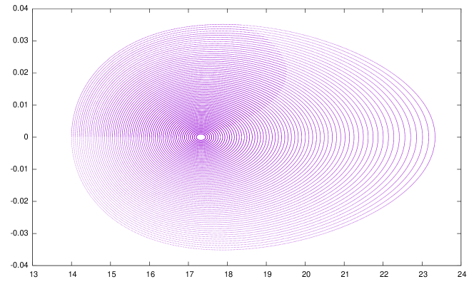
Figure 1: Energy $h=0.01$. Regular trajectories.

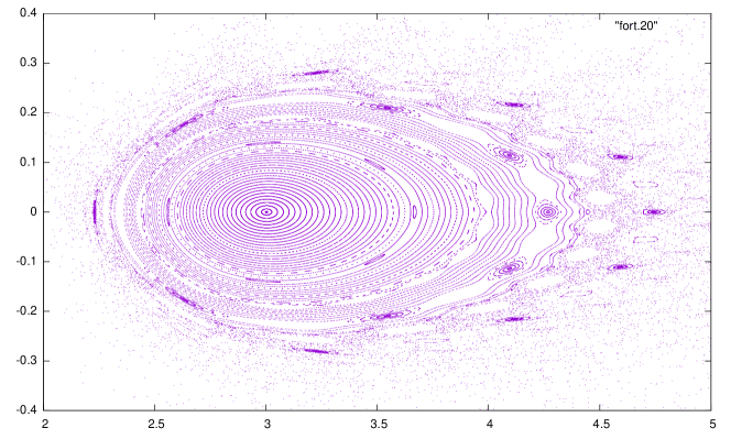
Figure 2: Energy $h=0.332412099$. There is a large chaotic zone, with escaping trajectories.

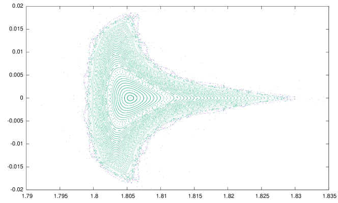
Figure 3: Energy $h=0.806$. Even larger chaotic/escaping zone. The triangular feature is probably related to a 3:1 torus resonance. Note that we zoomed in with respect to Fig.2.

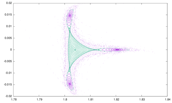
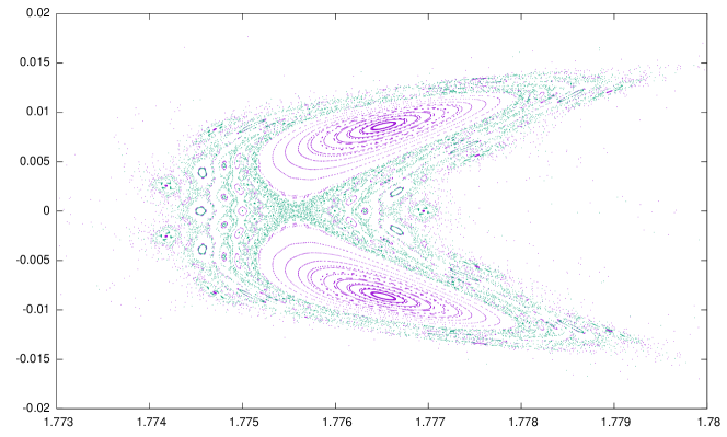
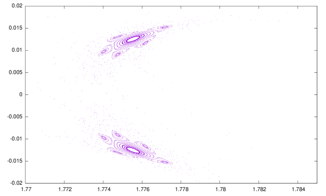
Figure 4: Nearby energies $h=0.8065,\,0.818,\,8189$. Only a small $a$ interval was depicted for better visualization. Which bifurcations took place: pitchfork, period doubling, Hamiltonian Hopf?

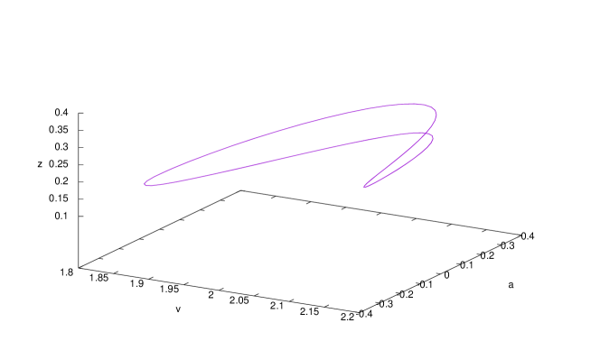
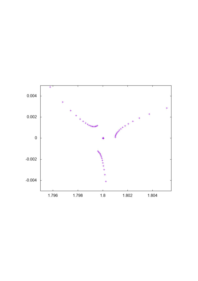
Figure 5: The periodic trajectory in the energy level $h=0.808$. Note the central zone shrinking in the associated surface of section

Understanding the dynamics near the equators is important both conceptually and numerically (see figs 6.1 and 6.2 in [79]). Linearization does not help. It is easy to see from the general cubic spline equation (19) that for any Riemannian metric geodesics whose accelerations vary linearly are $L^{2}$ splines. Our original (uninformed) guess was that, for any Riemannian manifold, splines would tend to accelerating geodesics as $t\rightarrow\pm\infty$.

Our numerical experiments indicate that this is not the case for cubic splines on $S^{2}$. They strongly suggest that the system is non-integrable. However, we found zones in the reduced phase space having invariant tori.

Surface of sections

In Figures 1 to 4 we depict some Poincaré sections of phase space $(v,a,\theta,z)$, taking $\theta=\pi/2$. The vertical axis is $a$, horizontal $v$. The parameters are $\beta=1,r=2,\mu=2$. Figure 5 shows a central periodic trajectory.

Invariant tori

Figs.6 and 7 depict invariant tori. They were found, among several others with complicated Lagrangian projections, by (obsessive) trial and error experimentation. They live on remote regions of phase space, neither close to the loxodromic equilibria nor to the equators $z=\pm 1$. There is a variety of confined trajectories whose ‘morphology’ merit further study.

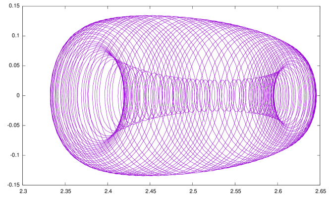
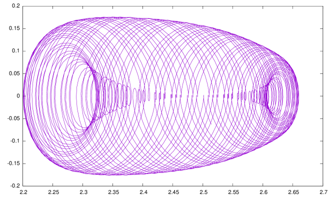
Figure 6: Invariant tori, seen on a Lagrangian projection in the plane $(a,z)$. Energies  $h=0.49494873,\,$ and $h=0.522397316$.

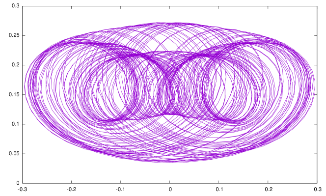
Figure 7: An invariant torus, seen on a Lagrangian projection in the plane $(a,z)$. $h=0.586204019$, $\beta=1,\mu=r=2$.

Trajectories emanating from the focus-focus

The simulations suggest that (at least some of them) are reaching a neighborhood of an equator. Will they eventually recur back to the focus-focus loxodromic equilibrium (figure eights of the unreduced)? Our simulations suggest that as $t\rightarrow\infty$ those trajectories seem to ‘orbit’ around the equator $z=-1$, but they stay at a ‘safe’ distance to it (see Figure 8).

We assert that this is not an artifact of the integrator. Here’s an heuristic argument. From (48) it follows that when $v\rightarrow\infty$ then $\dot{\theta}\sim v/r$, and $\theta$ also diverges (only more so). Therefore $\dot{z}=O(v^{-2})\rightarrow 0$ is an ever oscillatory way. This suggests that $z$ perhaps could stabilize close to $z=-1$, but at a distance of it.

A study of (48) is in order. The behavior of the systems for moderate values of $v$ seems quite unpredictable.

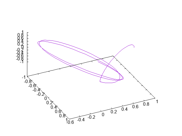
Figure 8: Top: reconstructed trajectory in the physical sphere, that approaches a neighborhood of an equator. Below: the reduced trajectory emanating from the unstable equilibrium, projected in the $(v,a)$ plane. Note that $v$ is growing quadratically with respect to $a$. The reconstructed trajectory is approaching a neighborhood of an equator. It remains to be seen if it stays there or returns to a vicinity of the reduced equilibrium.

3.4 Zero velocities and the relation to the general approach via split variables

Motivation: unfolding $v=0$

The price we had to pay in the description given so far of cubic splines in $S^{2}$ is that the scalar velocity $v$ appears in denominators of (3.1), and it may vanish along a solution in finite time. Nonetheless, we expect that this is regularizable. In other words, we posit that troubles at $v=0$ are (unfortunate) artifacts of our parameterization of $TS^{2}$ which excludes zero velocities and, ultimately, of the reduction procedure we implemented. (Notice that the lifted $SO(3)$ action on $TS^{2}$ is not principal; it is so when restricted to $M=TS^{2}-0$.)

We must then go back to the beautiful equations (2.2) for the unreduced system (taking $n=2$ there). As mentioned earlier, these were originally derived by Crouch and Leite [34, 33] (we also obtained them from our general split variables recipe in section 2.2). Clearly, unreduced solutions pass through ${\bf v}=x_{1}=0$ as smoothly as anywhere else.

Regularization consists in lifting a reduced solution such that $v(t_{o})=0$ to an unreduced solution. In Crouch-Leite system there is no trouble passing though $x_{1}(t_{o})=0$, and projecting back the continued unreduced solution. In Proposition 8 below we will provide the explicit Poisson map relating the unreduced split variables $(x_{o},x_{1},x_{2},x_{3})$ to the reduced ones $(a,v,M_{1},M_{2},M_{3})$.

Regularizing the reduced systems directly?

Before moving on to relating the unreduced and reduced system, we mention the following heuristic argument. Take the generic situation that $x_{2}(t_{o})\neq 0$ when $x_{1}(t_{o})=0$. Then

$$x_{1}\sim x_{2}(t_{o})(t-t_{o})\,\,{\rm for}\,\,t\,\,{\rm near}\,\,t_{o}.$$

This has a dramatic consequence in our reduction: $e_{1}=x_{1}/|x_{1}|$ sudenly flips from $-x_{2}(t_{o})/|x_{2}(t_{o})|$ to $+x_{2}(t_{o})/|x_{2}(t_{o})|$. In this case we argue that the continuation of (3.1) beyond $t_{o}$ could be done using the velocity reversal symmetry of the problem.

One indication is the behavior of the infinitesimal rotation (26) as $t\rightarrow t_{o}^{-}$. We have $\Omega=(0,v/r,u_{2}/v)\rightarrow(0,0,\infty)\,\,\,.$

We expect that this “infinite infinitesimal rotation” around $e_{3}$ will amount to an instantaneous rotation by $\pi$ of the tangent plane. In other words, the vectors $e_{1},e_{2}$ will instantaneously change sign at $t_{o}$, that is,

$$e_{1}^{+}=-e_{1}^{-},\,e_{2}^{+}=-e_{2}^{-}\,.$$

Indeed, in view of (52)

$$\int_{t_{o}^{-}}^{t_{o}^{+}}(u_{2}/v)dt=\int_{t_{o}^{-}}^{t_{o}^{+}}\,(\kappa_{g}v)\,dt=\int_{s_{o}^{-}}^{s_{o}^{+}}\kappa_{g}\,ds$$

and we posit that $\kappa_{g}$ should be $\pi$ times the delta function at $s_{o}=s(t_{o})$.

The Poisson map $(x,{\bf v},p,\alpha)\to(a,v,M_{1},M_{2},M_{3})$

We need to compute the composition

$$q^{*}(T^{*}S^{2})\oplus_{(TS^{2}-0)}q^{*}(T^{*}S^{2})\overset{(i)}{\simeq}T^{*}(TS^{2}-0)\overset{(ii)}{\simeq}T^{*}M\overset{(iii)}{\to}M_{red}.$$

The symplectomorphism $(i)$ is the $\psi_{\nabla}$ of section 2.1, with underlying change of variables given in proposition 3 (in the particular case of the $(n=2)$-sphere). The symplectomorphism $(ii)$ is induced by the diffeomorphism (24) between $TS^{2}-0$ and $M=\mathbb{R}_{+}\times SO(3)$ (see also appendix B). The Poisson map $(iii)$ is just the projection which forgets the $R\in SO(3)$ (once we use left trivialized covectors: $T^{*}SO(3)\simeq SO(3)\times\mathbb{R}^{3}$).
A straightforward tracking the above maps yields our final result (for simplicity we took $r=\beta=1$).

Proposition 8.

The above Poisson map taking the split variables $(x,\,{\bf v},\,p,\,\alpha)$ for $T^{*}(TS^{2})$, as described in proposition 3, to the reduced variables $(a,v,M_{1},M_{2},M_{3})\in M_{red}=T^{*}\mathbb{R}_{+}\times\mathbb{R}^{3}$ is given by

$$a = \alpha\cdot{\bf v}/v\,\,\,,\,\,\,v=|{\bf v}|$$

$$M_{1} = {\rm det}(p,{\bf v}/v,x)$$

$$M_{2} = \,\,\,p\cdot{\bf v}/v$$ (49)

$$M_{3} = {\rm det}(\alpha,\,x,\,{\bf v}).$$

4 Comments and further questions

Control systems on anchored vector bundles

More generally than in (1), which is a control problem with state space $A=TQ$, one could consider control problems with state space $A\ni(x,a)$ being a vector (or, more generally, affine) bundle $q:A\to Q$ with a connection $\nabla$, and state equations of the form

$$\dot{x}=\rho(a),\ \nabla_{\dot{x}}a=u$$

with $\rho:A\to TM$ a given (’anchor’) map. In this paper, we have been considering the particular case $A=TQ$ and $\rho=id$. Also note that for $u=0$ (uncontrolled problem) we recover the geodesic equations relative to $(\rho,\nabla)$.

Examples of such systems arise from nonholonomic control problems [21] and control on (almost) algebroids [55] (for background on algebroids, see also [69], [100], [35]). We observe that control problems with state space $TQ$ with a Levi-Civita connection can be recast, via the dual connection, to a control problem with state space $T^{*}Q$. This is a usefull observation for landmark splines, since the problem is best described in terms of a cometric.

In general, the PMP leads to the cotangent bundle $T^{*}A$ and to the problem of finding the optimal hamiltonian. The connection $\nabla$ allows us to obtain split variables generalizing those of section 2.1,

$$T^{*}A\simeq q^{*}(T^{*}Q)\oplus_{A}q^{*}A^{*}.$$

Proposition 1 generalizes to this more general setting and provides a formula for the symplectic structure in split variables (also containing curvature terms). Moreover, the optimal hamiltonian is easy to find in these variables just as in 2.1. This will be detailed in [7].

Higher order splines and natural curvatures

For future work one can think of higher order splines as a control problem with state equation corresponding to

$$\nabla^{(k+1)}_{\dot{x}}\dot{x}=u.$$

The state space can be taken to be $A=J^{k}Q$, the space of $k$-jets on $Q$. The cost functional can depend on $u$ and (possibly) lower order covariant derivatives $D^{(i)}_{\dot{q}}\dot{q}\,,\,i=1,\cdots k$. An optimal curve $\gamma(t)$ should connect two prescribed $k$-jets $j^{(k)}|_{x_{o}},\,j^{(k)}|_{x_{1}}\,\,$ (in computational anatomy it is often required that $\gamma(t)$ passes through a number of intermediary points at prescribed times). In this paper, we have treated the case $k=1$.

We remark that such a system is related to two very nice papers by Gay-Balmaz, Holm, Meier, Ratiu, and Vialard [46, 47] on higher order lagrangians.

Our general approach via PMP applies here as well. One obtains $T^{*}(J^{k}(Q))$ and has to find the optimal hamiltonian. At this point, one notices that $J^{k}(Q)$ fits into a tower of affine bundles

$$\cdots J^{k}(Q)\rightarrow J^{(k-1)}(Q)\rightarrow\cdots\rightarrow J^{1}(Q)\rightarrow Q,$$

see [65]. One can thus find split variables for $T^{*}(J^{k}(Q))$ recursively using a given connection on $J^{1}Q=TQ$. The higher order curvatures of the underlying curve $\gamma(t)\in Q$ will be related to components of the control, similarly to what we obtained in appendix B for $Q$ a surface (and $k=1$) and, more generally, to what happens in elastica (see e.g. [64], [56, 57]). We plan to pursue this in a sequel paper.

Is accessibility an issue?

For the general context of accessibility in mechanical control problems, see [9]. In Alan Weinstein’s Ph.D. dissertation [99], about cut and conjugate loci on Riemannian manifolds, there is basic lemma stating that, if the manifold is complete, connected, and of finite volume, then any two unit tangent vectors can be joined by a smooth curve, parametrized by arc length, with geodesic ends, having geodesic curvature smaller than any arbitrarily small bound. Using this result it is easy to show accessibility for the time-minimal, bounded acceleration problem. We wonder if the same is true in higher order, namely joining two given 2-jets by a curve with arbitrarily small “jerk”.

Controllability on vector bundles

In the seminal paper by Lewis and Murray [67] on configuration controllability of mechanical systems, the concept of symmetric product of vector fields was introduced. Their results were extended to mechanical systems with constraints and symmetries, see [31]. For a geometric interpretation, see [8]. Can the techniques be used in the general context of control problems on vector bundles with connection? Note that the control appears in a fraction ${\rm rank}(A)/({n+{\rm rank}(A)})$ of the equations (further, the system can be sub-actuated). For results on controlabillity of affine connection mechanical systems, see [10].

Diffusion PCA

More generally, on any framework where the phase space is a cotangent bundle $T^{*}P$ of a manifold with a bundle structure $P\to B$ (and a connection), a splitting of variables will be useful. In the case of principal bundles $G\to P\to P/G$, the reduction of $T^{*}P$ goes back to Kummer [62, 63] in the 1980’s. For instance, a theory for diffusion principal component analysis (PCA) was developed by Sommer [93], based upon stochastic development via Eells-Elworthy-Malliavin construction of Brownian motion [38], [94]. A Hamiltonian system on the cotangent bundle of the frame bundle $T^{*}({\rm Fr}(Q))$, governs the most probable paths.

Interpreting the terms in the (simple splines) Hamiltonian equations

Peter Michor observed at the workshop that the extra terms in the equation for $\dot{p}_{i}$ in Proposition 1 could be related to the concepts of symmetrized force and shape stress in his work with Michelli and Mumford [73].

$L^{\infty}$ vs. $L^{2}$

For certain applications, Noakes has argued that $L^{\infty}$ could be better than $L^{2}$. Indeed, from the mathematical side, a drawback of cubic splines is that for manifolds of negative curvature the velocity can become infinite in finite time [82]. One can anticipate this behavior from equations (13). They contain curvatures - signs matter. In contradistinction, under bounded acceleration constraint, the scalar velocity grows at most linearly, so in all cases trouble is avoided by default. Would that be physiologically reasonable? Some simple experiments with $n=d=1$ shows that, for cubic splines, the acceleration can attain high values of during the prescribed time interval, while the time minimal bounded acceleration can do the job in not a much longer time, depending on the concrete problem at hand. For robotics applications, or for an athlete, disastrous consequences could happen if the norm of the control force exceeds a given bound at some instant, see [96], [92].

Singular reduction

$SO(3)$ does not act freely on $TS^{2}$: trouble happens when the scalar velocity $v$ vanishes (ie., the zero section of $TS^{2}$), and this propagates to non-freeness of the action of $SO(3)$ on the symplectic manifold $T^{*}(TS^{2})$. More generally, one may consider a vector bundle $A\to Q$ with a $G$-action, that is not free on the base (hence on the zero section). A procedure to do the singular Hamiltonian reduction of $T^{*}A$ is in order, a research direction that we hope to address in the future.

Applying Morales-Ramis theory

Let us go back to cubic splines in $S^{2}$ as described in section 3. Since the kissing circles unstable periodic orbits are explicitly known, one may hope to prove nonintegrability using the Morales-Ramis approach [74]. However, linearizing (2.2) and doing the required Galois theory for the time periodic linear equations would be, no doubt, a tour-de-force. On could also attempt to show nonintegrability linearizing around the equator solutions.

Controlled Lagrangians

In [20, 19] the concept of controlled Lagrangian is introduced, for mechanical systems $L=T-V$ of natutal type. The control forces here keep the conservative nature of the controlled system. This is achieved by conveniently shaping the kinetic and/or potential energy. The modified system is still a closed-loop system, and the controlled system is Lagrangian by construction. Energy methods are used to find control gains that yield closed-loop stability. It would be interesting to see if such methods could be used to match tangent vectors.

Splines in infinite dimensional Riemannian geometry

This is a special edition about a meeting on infinite-dimensional Riemannian geometry, so we now try to link the present work to the infinite dimensional setting. As it is customary, the idea is to use the present study of systems with underlying finite dimensional configuration spaces $Q$ as simplified models for the cases in which $Q$ is an infinite dimensional Riemannian manifold. In this direction, the Levi-Civita connection and the curvature of Sobolev metrics on $Q={\rm Diff}$ have been studied by several authors, see eg. [14], [72], [48], [59, 6, 60], [75]. Below we enumerate some related questions.

1. PDEs for splines in shape space. This means optimal control problems with state space $A=T{\rm Diff}$. In order to describe $T(T{\rm Diff})$ and $T^{*}(T{\rm Diff})$, one can take advantage of the fact that ${\rm Diff}$ is a group and, thus, $T{\rm Diff}={\rm Diff}\times\mathcal{X}$. What are the corresponding PDEs for $L^{2}$ and $L^{\infty}$ splines? They should involve not only the momentum density ${\bf m}$ but another density $\bf{p}$ corresponding to a Pontryagin multiplier (alternatively, a PDE for ${\bf m}$ involving three time derivatives).

2. Lifting landmark splines. Consider splines on a finite dimensional landmark space, i.e., with state space $A=T(\mathbb{R}^{d})^{N}$ and cometric given by a Green function $G(x,y)$. In the case of a finite number $N$ of (point) landmarks, Mario Michelli [71, 72] has implemented the geodesic equations for the landmark cometrics. In a similar way as it can be done for EPDiff, can these be lifted to solutions of a corresponding infinite dimensional spline problem on $T{\rm Diff}$? Faute de mieux, one would use the same ansatz (6) to move other points in $\mathcal{D}$, but in doing so we would be neglecting the new costate variables. Once this question is elucidated, one could proceed to numerical discretization, see e.g. [30], [11], [83] for geodesics in ${\rm Diff}$.

Acknowledgements. Supported by Brazil’s Science without Frontiers grants on Geometric Mechanics and Control, PVE011-2012 and PVE089-2013. We thank Darryl Holm, Tudor Ratiu and Richard Montgomery and Alain Albouy for their generous participation in the project and Marco Castrillon for useful discussions. JK wishes to thank Martins Bruveris, Martin Bauer and Peter Michor for the invitation to the Program on Infinite-Dimensional Riemannian Geometry with Applications to Image Matching and Shape Analysis at the Erwin Schrodinger Institute.

Appendix A Fortran program for reconstruction

      implicit real*8(a-h,o-z)
      dimension z(13),b(13),f(13),r(13,13)
      common erk,amu,beta,rr
      external dertres
      erk=1.d-13
      n=13

c     parameters
      rr=2.d0
      amu=2.d0
      beta=1.d0
      pi=4.0*datan(1.d0)


c   variables are in order 1 to 13:
c   r13 r23 r33  r11 r21 r31 r12 r22 r32    v  a  tetha phi

c initial conditions
Ψ z(1)=0.d0
Ψ z(2)=0.d0
Ψ z(3)=1.d0
Ψ z(4)=1.d0
Ψ z(5)=0.d0
Ψ z(6)=0.d0
Ψ z(7)=0.d0
Ψ z(8)=1.0d0
Ψ z(9)=0.d0
Ψ z(10)=(amu*rr/(beta*dsqrt(2.d0)))**(1./3)
Ψ z(11)=0.0d0
Ψ z(12)=pi/2.d0
Ψ z(13)=pi/4.d0
c
      t=0.d0
      e=erk
      n=13
      h=.01d0
      hmi=1.d-8
      hma=.1d0
cΨ
      do i=1,200
Ψ  call rk78n(t,z,n,h,hmi,hma,e,r,b,f,dertres)Ψ
Ψ  write(20,*)z(1),z(2),z(3)
Ψ  write(21,*)z(10),z(11),z(12),z(13)
      enddo
      stop
      end

C--------------------------------------------------------------------
C   FORTRAN SUBROUTINE FOR  EDOS
C-------------------------------------------------------------------


c  Runge Kutta code courtesy of C. SIMO group

 subroutine dertres(a,b,n,f)
      implicit real*8(a-h,o-z)
      dimension b(13),f(13)
      common erk,amu,beta,rr
Ψ vr=b(10)/rr
Ψ vb=beta*b(10)**2
Ψ am3=amu*dcos(b(13))*dsin(b(12))
      f(1)=vr*b(4)
      f(2)=vr*b(5)
      f(3)=vr*b(6)
      f(4)=am3*b(7)/(vb)-b(1)*vr
      f(5)=am3*b(8)/(vb)-b(2)*vr
      f(6)=am3*b(9)-b(3)*vr
      f(7)=-am3*b(4)/(vb)
      f(8)=-am3*b(5)/(vb)
      f(9)=-am3*b(6)/(vb)
      f(10)=b(11)/beta
      f(11)=-amu*dsin(b(13))/rr+amu**2*dcos(b(13))*dsin(b(12))**2/
     #Ψ (beta*b(10)**3)
      f(12)=(b(10)/(rr)-amu*(sin(b(12)))**2*dsin(b(13))/(beta*b(10)**2))
      f(13)=-amu*dcos(b(13))*dsin(b(12))*dcos(b(12))/(beta*b(10)**2)
      return
      end
    

Appendix B State equations on convex surfaces and the Gauss map

In this appendix, we elaborate on a description of non-zero tangent vectors on a convex surface $\Sigma$ which uses the Gauss map. We use it to provide an alternative form of the state equations (7) on $T\Sigma$. This description is used in section 3 in the particular case of $\Sigma=S^{2}$ to exploit the rotational symmetry.

Let $\Sigma\subset\mathbb{R}^{3}$ be a closed smooth convex surface. The Gauss map induces a diffeomorphism between $T\Sigma-0$ and $\mathbb{R}_{+}\times SO(3)$:

$${\bf v}_{q}\,\leftrightarrow\,\,(v,R)\,\,\,,\,\,\,\,\,v=||{\bf v}_{q}||\neq 0$$ (50)

where $R\in SO(3)$ is constructed as follows: points $q\in\Sigma$ correspond uniquely to external unit normal vectors to the surface, which we denote $e_{3}$. Now, a nonzero tangent vector ${\bf v}_{q}$ corresponds uniquely to a pair $(v,e_{1})$ with

$${\bf v}_{q}=v\,e_{1}\,\,,\,\,v>0\,\,\,,\,\,{\rm and}\,\,\,e_{1}\cdot e_{3}=0\,\,,\,\,|e_{1}|=|e_{3}|=1.$$

We use a redundant vector $e_{2}=e_{3}\times e_{1}$ to construct the matrix $R$ with columns $e_{1},e_{2},e_{3}$. Therefore, a control problem with state space $T\Sigma$ corresponds to a control problem on $SO(3)\times R_{+}$, provided we exclude the zero section.

Let us now move on to rewritting the state equations (7) in our present situation. Recall the Darboux formulas for a curve $\gamma(s)\in\Sigma$ (${}^{\prime}=d/ds$)

$$e_{1}^{\prime}=\kappa_{g}\,e_{2}+\kappa_{n}\,e_{3}\,,\quad e_{2}^{\prime}=-\kappa_{g}\,e_{1}+\tau_{g}\,e_{3}\,,\quad e_{3}^{\prime}=-\kappa_{n}\,e_{1}-\tau_{g}\,e_{2}$$

where $\kappa_{g}$ is the geodesic curvature, $\kappa_{n}$ the normal curvature, and $\tau_{g}$ the geodesic torsion of $\gamma$. These formulas can be rewritten as

$$\dot{R}=R\,X\quad\mbox{with}\quad X=v\,\left(\begin{array}[]{ccc}0&-\kappa_{g}&-\kappa_{n}\\ \kappa_{g}&0&-\tau_{g}\\ \kappa_{n}&\tau_{g}&0\end{array}\right).$$

The normal curvature is not freely controllable since it corresponds to the force that constrains the curve to stay in the surface. Indeed, taking derivatives in the ambient space,

$$\ddot{\gamma}=\dot{v}\,e_{1}+v^{2}\,e_{1}^{\prime}=\dot{v}\,e_{1}+v^{2}(\kappa_{g}\,e_{2}+\kappa_{n}\,e_{3})=\nabla_{\dot{\gamma}}\,\dot{\gamma}+v^{2}\kappa_{n}\,e_{3}$$

with $\kappa_{n}=e_{1}^{\prime}\cdot e_{3}=-e_{3}^{\prime}\cdot e_{1}:=B(e_{1},e_{1})$ where $B$ is the second fundamental form of the surface. On the other hand, the intrinsic description of the state equations, using the Levi-Civita connection, reads

$$\nabla_{\dot{\gamma}}\,\dot{\gamma}=\,u_{1}\,e_{1}+u_{2}\,e_{2}$$ (51)

where $u_{1},u_{2}$ are the controls. The previous simple calculation thus showed that

$$u_{1}=\dot{v}\quad\mbox{and}\quad u_{2}=v^{2}\kappa_{g}.$$ (52)

But the geodesic torsion $\kappa_{g}$ also admits the following interesting formula found by Darboux

$$\tau_{g}=\tau_{g}(e_{1})=(\kappa_{1}-\kappa_{2})\sin\phi\,\cos\phi$$ (53)

where $\phi$ is the angle between the unit tangent vector $e_{1}$ to the curve and a principal direction on the surface. We then conclude that the state equations can be written as

$$\dot{v}=u_{1}\,,\quad\dot{R}=R\,X\,,\quad X=\left(\begin{array}[]{ccc}0&-u_{2}/v&-v\,B(e_{1},e_{1})\\ u_{2}/v&0&-v\,\tau_{g}(e_{1})\\ v\,B(e_{1},e_{1})&v\,\tau_{g}(e_{1})&0\end{array}\right)\,.$$ (54)

References

- [1] L. Abrunheiro, M. Camarinha and J. Clemente-Gallardo, Cubic polynomials on Lie groups: reduction of the Hamiltonian system, Journal of Physics A: Mathematical and Theoretical, 44 (2011), 355203, URL \urlhttp://stacks.iop.org/1751-8121/44/i=35/a=355203.
- [2] L. Abrunheiro, M. Camarinha and J. Clemente-Gallardo, Corrigendum: Cubic polynomials on Lie groups: reduction of the Hamiltonian system, Journal of Physics A: Mathematical and Theoretical, 46 (2013), 189501, URL \urlhttp://stacks.iop.org/1751-8121/46/i=18/a=189501.
- [3] L. Abrunheiro and M. Camarinha, Optimal control of affine connection control systems from the point of view of lie algebroids, International Journal of Geometric Methods in Modern Physics, 11 (2014), 1450038, URL \urlhttp://www.worldscientific.com/doi/abs/10.1142/S0219887814500388.
- [4] L. Abrunheiro, M. Camarinha and J. Clemente-Gallardo, Geometric Hamiltonian formulation of a variational problem depending on the covariant acceleration, Conference Papers in Mathematics, 2013 (2013), 9, URL \urlhttp://www.hindawi.com/archive/2013/243621/.
- [5] A. Attri, Development of Models for the Equations of Motion in the Solar System: Implementations and Applications, Master’s thesis, Universitat Politécnica de Catalunya Master in Aerospace Science and Technology, 2014.
- [6] B. B. Khesin, J. Lenells, G. Misiolek and S. C. Preston, Curvatures of Sobolev metrics on diffeomorphism groups, Pure and Applied Mathematics Quarterly, 9 (2013), 291–332.
- [7] P. Balseiro, A. Cabrera and J. Koiller, Optimal control on vector bundles, in preparation.
- [8] M. Barbero-Liñán and A. D. Lewis, Geometric interpretations of the symmetric product in affine differential geometry and applications, International Journal of Geometric Methods in Modern Physics, 09 (2012), 1250073, URL \urlhttp://www.worldscientific.com/doi/abs/10.1142/S0219887812500739.
- [9] M. Barbero-Liñán, Characterization of accessibility for affine connection control systems at some points with nonzero velocity, in Proceedings of the IEEE Conference on Decision and Control and European Control Conference, 2011, 6528–6533.
- [10] M. Barbero-Liñán and M. Sigalotti, High-order sufficient conditions for configuration tracking of affine connection control systems, Systems & Control Letters, 59 (2010), 491–503, URL \urlhttp://www.sciencedirect.com/science/article/pii/S0167691110000757 (http://arxiv.org/abs/1501.04026).
- [11] M. Bauer, M. Bruveris, P. Harms and J. Moller-Andersen, A numerical framework for Sobolev metrics on the space of curves. SIAM J. Imaging Sci. (forthcoming), arxiv:1603.03480.
- [12] M. Bauer, M. Bruveris, P. Harms and J. Møller-Andersen, Curve Matching with Applications in Medical Imaging, 5th MICCAI workshop on Mathematical Foundations of Computational Anatomy, arXiv:1506.08840.
- [13] M. Bauer, M. Bruveris and P. W. Michor, Why use Sobolev metrics on the space of curves, in Riemannian Computing in Computer Vision, chapter 11, Turaga, P. and Srivastava, A., editors, p. 223-255, Springer-Verlag, 2016.
- [14] M. Bauer, M. Bruveris and P. Michor, Overview of the geometries of shape spaces and diffeomorphism groups, Journal of Mathematical Imaging and Vision, 50 (2014), 60–97, URL \urlhttp://dx.doi.org/10.1007/s10851-013-0490-z.
- [15] M. Bauer, M. Eslitzbichler and M. Grasmair, Landmark-guided elastic shape analysis of human character motions, arxiv:1502.07666.
- [16] M. Bauer, P. Harms and P. W. Michor, Sobolev metrics on shape space of surfaces, Journal of Geometric Mechanics, 3 (2011), 389–438, URL \urlhttp://aimsciences.org/journals/displayArticlesnew.jsp?paperID=7061.
- [17] M. Bauer, P. Harms and P. W. Michor, Sobolev metrics on shape space, ii: Weighted sobolev metrics and almost local metrics, Journal of Geometric Mechanics, 4 (2012), 365–383, URL \urlhttp://aimsciences.org/journals/displayArticlesnew.jsp?paperID=8178.
- [18] C. Bingham, Review: Geoffrey S. Watson, Statistics on Spheres, Ann. Statist., 13 (1985), 838–844, URL \urlhttp://dx.doi.org/10.1214/aos/1176349566.
- [19] A. Bloch, D. E. Chang, N. Leonard and J. Marsden, Controlled Lagrangians and the stabilization of mechanical systems. II. potential shaping, Automatic Control, IEEE Transactions on, 46 (2001), 1556–1571.
- [20] A. Bloch, N. Leonard and J. Marsden, Controlled Lagrangians and the stabilization of mechanical systems. I. the first matching theorem, Automatic Control, IEEE Transactions on, 45 (2000), 2253–2270.
- [21] A. Bloch, Nonholonomic Mechanics and Control, vol. 24 of Interdisciplinary Applied Mathematics, Springer, 2007.
- [22] M. Bruveris, Geometry of Diffeomorphism Groups and Shape Matching, PhD thesis, Department of Mathematics, Imperial College, london, 2012.
- [23] M. Bruveris and D. Holm, Geometry of Image Registration: The Diffeomorphism Group and Momentum Maps, in Geometry, Mechanics, and Dynamics: The Legacy of Jerry Marsden, ed. by Chang, D.E., Holm, D.D., Patrick, G., Ratiu, T., vol. 73 of Fields Institute Communications Series, Springer-Verlag, 2015, 19–56.
- [24] F. Bullo and A. D. Lewis, Geometric Control of Mechanical Systems, Texts in Applied Mathematics 49, Springer-Verlag, New York, 2005.
- [25] F. Bullo and A. D. Lewis, Supplementary chapters for Geometric Control of Mechanical Systems, motion.mee.ucsb.edu/book-gcms, 2014.
- [26] C. L. Burnett, D. D. Holm and D. M. Meier, Inexact trajectory planning and inverse problems in the Hamilton–Pontryagin framework, Proceedings of the Royal Society of London A: Mathematical, Physical and Engineering Sciences, 469.
- [27] A. Castro and J. Koiller, On the dynamic Markov-Dubins problem: From path planning in robotics and biolocomotion to computational anatomy, Regular and Chaotic Dynamics, 18 (2013), 1–20, URL \urlhttp://dx.doi.org/10.1134/S1560354713010012.
- [28] D. E. Chang, A simple proof of the Pontryagin maximum principle on manifolds, Automatica, 47 (2011), 630 – 633, URL \urlhttp://www.sciencedirect.com/science/article/pii/S0005109811000525.
- [29] A. Chenciner and R. Montgomery, A remarkable periodic solution of the three-body problem in the case of equal masses., Annals of Mathematics. Second Series, 152 (2000), 881–901, URL \urlhttp://eudml.org/doc/121861.
- [30] A. Chertock, P. D. Toit and J. E. Marsden, Integration of the EPDiff equation by particle methods,, ESAIM: Mathematical Modelling and Numerical Analysis, 46 (2012), 515–534.
- [31] J. Cortés, S. Martínez, J. P. Ostrowski and H. Zhang, Simple mechanical control systems with constraints and symmetry, SIAM Journal on Control and Optimization, 41 (2002), 851–874, URL \urlhttp://dx.doi.org/10.1137/S0363012900381741.
- [32] P. Crouch, F. S. Leite and M. Camarinha, A second order Riemannian variational problem from a Hamiltonian perspective, preprint, Centro de Matemática da Universidade de Coimbra, http://hdl.handle.net/10316/11230, 1998.
- [33] P. Crouch and F. Leite, The dynamic interpolation problem: On Riemannian manifolds, Lie groups, and symmetric spaces, Journal of Dynamical and Control Systems, 1 (1995), 177–202, URL \urlhttp://dx.doi.org/10.1007/BF02254638.
- [34] P. Crouch and F. S. Leite, Geometry and the dynamic interpolation problem, in Proceedings of the 1991 American Control Conference, 1991, 1131–1136.
- [35] M. de León, J. C. Marrero and E. Martínez, Lagrangian submanifolds and dynamics on Lie algebroids, Journal of Physics A: Mathematical and General, 38 (2005), R241, URL \urlhttp://stacks.iop.org/0305-4470/38/i=24/a=R01.
- [36] N. Desai, S. Ploskonka, L. R. Goodman, C. Austin, J. Goldberg and T. Falcone, Analysis of embryo morphokinetics, multinucleation and cleavage anomalies using continuous time-lapse monitoring in blastocyst transfer cycles, Reproductive Biology and Endocrinology : RB&E, 12 (2014), 54–54, URL \urlhttp://www.ncbi.nlm.nih.gov/pmc/articles/PMC4074839/.
- [37] I. L. Dryden, Statistical analysis on high-dimensional spheres and shape spaces, The Annals of Statistics, 33 (2005), 1643–1665, URL \urlhttp://www.jstor.org/stable/3448620.
- [38] D. Elworthy, Geometric aspects of diffusions on manifolds, in École d’Été de Probabilités de Saint-Flour XV–XVII, 1985–87, Lecture Notes in Mathematics (ed. P.-L. Hennequin), vol. 1362, Springer Berlin Heidelberg, 1988, 277–425, URL \urlhttp://dx.doi.org/10.1007/BFb0086183.
- [39] E. Fehlberg, Classical Seventh, Sixth, and Fifth-Order Runge Kutta-Nystrom Formula with Stepsize Control for General Second-Order Differential Equations, Technical report, NASA TR R-432, Washington D.C, 1974.
- [40] J.-B. Fiot, H. Raguet, L. Risser, L. D. Cohen, J. Fripp and F.-X. Vialard, Longitudinal deformation models, spatial regularizations and learning strategies to quantify Alzheimer’s disease progression, NeuroImage: Clinical, 4 (2014), 718 – 729, URL \urlhttp://www.sciencedirect.com/science/article/pii/S2213158214000205.
- [41] N. Fisher, T. Lewis and B. Embleton, Statistical Analysis of Spherical Data, Cambridge University Press, 1987.
- [42] P. T. Fletcher, Statistical Variability in Nonlinear Spaces: Application to Shape Analysis and DT-MRI, PhD thesis, Department of Computer Science, University of North Carolina, 2004.
- [43] P. T. Fletcher, Geodesic regression and the theory of least squares on Riemannian Manifolds, International Journal of Computer Vision, 105 (2013), 171–185, URL \urlhttp://dx.doi.org/10.1007/s11263-012-0591-y.
- [44] D. Fortuné, J. A. R. Quintero and C. Vallée, Pontryagin calculus in Riemannian geometry, in Geometric Science of Information, Lecture Notes in Computer Science (eds. F. Nielsen, F. Barbaresco and F. Dubois), vol. 9389, Springer International Publishing, 2015, 541–549, URL \urlhttp://dx.doi.org/10.1007/978-3-319-25040-3_58.
- [45] B. Francis and M. Maggiore, Flocking and Rendezvous in Distributed Robotics, Springer International Publishing, 2016.
- [46] F. Gay-Balmaz, D. D. Holm, D. M. Meier, T. S. Ratiu and F.-X. Vialard, Invariant higher-order variational problems, Communications in Mathematical Physics, 309 (2012), 413–458, URL \urlhttp://dx.doi.org/10.1007/s00220-011-1313-y.
- [47] F. Gay-Balmaz, D. D. Holm, D. M. Meier, T. S. Ratiu and F.-X. Vialard, Invariant higher-order variational problems ii, Journal of Nonlinear Science, 22 (2012), 553–597, URL \urlhttp://dx.doi.org/10.1007/s00332-012-9137-2.
- [48] P. Harms, Sobolev metrics on shape space of surfaces, PhD thesis, Universität Wien, 2010.
- [49] J. Hinkle, P. Fletcher and S. Joshi, Intrinsic polynomials for regression on riemannian manifolds, Journal of Mathematical Imaging and Vision, 50 (2014), 32–52, URL \urlhttp://dx.doi.org/10.1007/s10851-013-0489-5.
- [50] J. Hinkle, P. Muralidharan, P. Fletcher and S. Joshi, Polynomial regression on Riemannian manifolds, in Computer Vision – ECCV 2012 (eds. A. Fitzgibbon, S. Lazebnik, P. Perona, Y. Sato and C. Schmid), vol. 7574 of Lecture Notes in Computer Science, Springer Berlin Heidelberg, 2012, 1–14, URL \urlhttp://dx.doi.org/10.1007/978-3-642-33712-3_1.
- [51] D. D. Holm, T. Schmah and C. Stoica, Geometric Mechanics and Symmetry: From Finite to Infinite Dimensions, Oxford Texts in Applied and Engineering Mathematics, Oxford University Press, 2009.
- [52] K. Hüper, Y. Shen and F. Silva Leite, Geometric splines and interpolation on : Numerical experiments, in Proceedings of the 45th IEEE Conference on Decision Control, San Diego, CA, USA, 2006, 6403–6407.
- [53] R. V. Iyer, Pontryagin’s minimum principle for simple mechanical systems on Riemannian manifolds and Lie groups, 2005, Http://www.math.ttu.edu/ rvenkata/Papers/max-principle.pdf.
- [54] R. V. Iyer, R. Holsapple and D. Doman, Optimal control problems on parallelizable Riemannian manifolds: theory and applications, ESAIM: Control, Optimisation and Calculus of Variations, 12 (2006), 1–11, URL \urlhttp://www.esaim-cocv.org/action/article_S1292811905000266.
- [55] M. Jóźwikowski, Optimal control theory on almost Lie algebroids, PhD thesis, Institute of Mathematics, Polish Academy of Sciences, 2011.
- [56] V. Jurdjevic, The Delauney-Dubins problem, in Geometric Control Theory and Sub-Riemannian Geometry (eds. G. Stefani, U. Boscain, J.-P. Gauthier, A. Sarychev and M. Sigalotti), Springer International Publishing, 2014, 219–239, URL \urlhttp://dx.doi.org/10.1007/978-3-319-02132-4_14.
- [57] V. Jurdjevic, Optimal Control and Geometry: Integrable Systems, Cambridge Studies in Advanced Mathematics, Cambridge University Press, 2016.
- [58] C. Y. Kaya and J. L. Noakes, Finding interpolating curves minimizing acceleration in the euclidean space via optimal control theory, SIAM Journal on Control and Optimization, 51 (2013), 442–464, URL \urlhttp://dx.doi.org/10.1137/12087880X.
- [59] B. Khesin, J. Lenells, G. Misiołek and S. Preston, Geometry of diffeomorphism groups, complete integrability and geometric statistics, Geometric and Functional Analysis, 23 (2013), 334–366, URL \urlhttp://dx.doi.org/10.1007/s00039-013-0210-2.
- [60] B. Khesin and R. Wendt, The Geometry of Infinite-Dimensional Groups, vol. 51 of Modern Surveys in Mathematics, 1st edition, Springer-Verlag Berlin Heidelberg, 2009.
- [61] J. Koiller and T. Stuchi, Time minimal splines on the sphere, submitted, in Proceedings of the Sixth IST-IME Meeting (September 5-9 2016, Lisbon), in honor of Waldyr Oliva, to appear.
- [62] M. Kummer, On the construction of the reduced phase space of a hamiltonian system with symmetry, Indiana Univ. Math. J., 30 (1981), 281–291.
- [63] M. Kummer, Realizations of the reduced phase space of a hamiltonian system with symmetry, in Local and Global Methods of Nonlinear Dynamics, Lecture Notes in Physics (eds. A. W. Sáenz, W. W. Zachary and R. Cawley), vol. 252, Springer Berlin Heidelberg, 1986, 32–39, URL \urlhttp://dx.doi.org/10.1007/BFb0018326.
- [64] J. Langer and D. A. Singer, The total squared curvature of closed curves, J. Differential Geom., 20 (1984), 1–22, URL \urlhttp://projecteuclid.org/euclid.jdg/1214438990.
- [65] A. D. Lewis, The affine structure of jet bundles, www.mast.queensu.ca/~andrew/notes/pdf/2005a.pdf, 2005.
- [66] A. D. Lewis, Aspects of Geometric Mechanics and Control of Mechanical Systems, PhD thesis, Caltech, http://www.mast.queensu.ca/ andrew/papers/pdf/1995f.pdf, 1995.
- [67] A. D. Lewis and R. M. Murray, Configuration controllability of simple mechanical control systems, SIAM Review, 41 (1999), 555–574, URL \urlhttp://dx.doi.org/10.1137/S0036144599351065.
- [68] M. Lewis, D. Offin, P.-L. Buono and M. Kovacic, Instability of the periodic hip-hop orbit in the -body problem with equal masses, Discrete and Continuous Dynamical Systems, 33 (2013), 1137–1155, URL \urlhttp://aimsciences.org/journals/displayArticlesnew.jsp?paperID=7827.
- [69] P. Libermann, Lie algebroids in mechanics, Archivum Mathematicum, 32 (1966), 147–162.
- [70] Z. Lin, B. Francis and M. Maggiore, Getting mobile autonomous robots to rendezvous, in Control of Uncertain Systems: Modelling, Approximation, and Design (eds. B. Francis, M. Smith and J. E. Willems), vol. 329, 2006, 119–137.
- [71] M. Micheli, P. W. Michor and D. Mumford, Sectional curvature in terms of the cometric, with applications to the Riemannian manifolds of landmarks, SIAM Journal on Imaging Sciences, 5 (2012), 394–433, URL \urlhttp://dx.doi.org/10.1137/10081678X.
- [72] M. Micheli, P. W. Michor and D. Mumford, Sobolev metrics on diffeomorphism groups and the derived geometry of spaces of submanifolds, Izvestiya: Mathematics, 77 (2013), 541, URL \urlhttp://stacks.iop.org/1064-5632/77/i=3/a=541.
- [73] P. W. Michor, Manifolds of mappings and shapes, http://arxiv.org/abs/1505.02359.
- [74] J. Morales Ruiz, Differential Galois Theory and Non-Integrability of Hamiltonian Systems, Modern Birkhäuser Classics, Springer-Verlag, 1999.
- [75] D. Mumford and P. W. Michor, On Euler’s equation and ‘EPDiff’, Journal of Geometric Mechanics, 5 (2013), 319–344, URL \urlhttp://aimsciences.org/journals/displayArticlesnew.jsp?paperID=9003.
- [76] P. Muralidharan, J. Fishbaugh, H. J. Johnson, S. Durrleman, J. S. Paulsen, G. Gerig and P. T. Fletcher, Diffeomorphic Shape Trajectories for Improved Longitudinal Segmentation and Statistics, 49–56, Springer International Publishing, https://www.ncbi.nlm.nih.gov/pubmed/25320781, 2014, URL \urlhttp://dx.doi.org/10.1007/978-3-319-10443-0_7.
- [77] M. Niethammer, Y. Huang and F.-X. Vialard, Geodesic regression for image time-series, in Medical Image Computing and Computer-Assisted Intervention – MICCAI 2011 (eds. G. Fichtinger, A. Martel and T. Peters), vol. 6892 of Lecture Notes in Computer Science, Springer Berlin Heidelberg, 2011, 655–662, URL \urlhttp://dx.doi.org/10.1007/978-3-642-23629-7_80.
- [78] L. Noakes, Spherical Splines, 77–101, in Geometric Properties for Incomplete Data, ed. by R. Klette, R. Kozera, R., L.Noakes and J.Weickert, Computational Imaging and Vision 31, Springer-Verlag, 2006.
- [79] L. Noakes, Approximating near-geodesic natural cubic splines, Communications in Mathematical Sciences, 12 (2014), 1409 – 1425.
- [80] L. Noakes, Minimum accelerations in Riemannian manifolds, Advances in Computational Mathematics, 40 (2014), 839–863, URL \urlhttp://dx.doi.org/10.1007/s10444-013-9329-9.
- [81] L. Noakes, G. Heinzinger and B. Paden, Cubic splines on curved spaces, IMA Journal of Mathematical Control and Information, 6 (1989), 465–473, URL \urlhttp://imamci.oxfordjournals.org/content/6/4/465.abstract.
- [82] M. Pauley and L. Noakes, Cubics and negative curvature., Differ. Geom. Appl., 30 (2012), 694–701.
- [83] D. Pavlov, Geometric Discretization of the EPDiff Equations, ArXiv e-prints 1503.03935.
- [84] L. S. Pontryagin, V. G. Boltyanskii, R. V. Gamkrelidze and E. F. Mishchenko, The Mathematical Theory of Optimal Processes, Interscience, 1962.
- [85] T. Popiel, Higher order geodesics in Lie groups, Mathematics of Control, Signals, and Systems, 19 (2007), 235–253, URL \urlhttp://dx.doi.org/10.1007/s00498-007-0012-x.
- [86] R. T. Rockafellar, Convex Analysis, Princeton Landmarks in Mathematics and Physics, Princeton University Press, 1996.
- [87] M. Ross, A Primer on Pontryagin’s Principle in Optimal Control, Collegiate Publishers, 2009.
- [88] C. Samir, P.-A. Absil, A. Srivastava and E. Klassen, A gradient-descent method for curve fitting on Riemannian manifolds, Foundations of Computational Mathematics, 12 (2012), 49–73, URL \urlhttp://dx.doi.org/10.1007/s10208-011-9091-7.
- [89] N. Singh and M. Niethammer, Splines for diffeomorphic image regression, in Medical Image Computing and Computer-Assisted Intervention – MICCAI 2014 (eds. P. Golland, N. Hata, C. Barillot, J. Hornegger and R. Howe), vol. 8674 of Lecture Notes in Computer Science, Springer International Publishing, 2014, 121–129, URL \urlhttp://dx.doi.org/10.1007/978-3-319-10470-6_16.
- [90] N. Singh, F.-X. Vialard and M. Niethammer, Splines for diffeomorphisms, Medical Image Analysis, 25 , 56–71, URL \urlhttp://dx.doi.org/10.1016/j.media.2015.04.012.
- [91] S. Smith, M. Broucke and B. Francis, Curve shortening and the rendezvous problem for mobile autonomous robots, Automatic Control, IEEE Transactions on, 52 (2007), 1154–1159.
- [92] M. H. Sohn, J. L. McKay and L. H. Ting, Defining feasible bounds on muscle activation in a redundant biomechanical task: practical implications of redundancy., J Biomech, 46 (2013), 1363–1368.
- [93] S. Sommer, Anisotropic distributions on manifolds: Template estimation and most probable paths, in Information Processing in Medical Imaging, Lecture Notes in Computer Science (eds. S. Ourselin, D. C. Alexander, C.-F. Westin and M. J. Cardoso), vol. 9123, Springer International Publishing, 2015, 193–204, URL \urlhttp://dx.doi.org/10.1007/978-3-319-19992-4_15.
- [94] S. Sommer, Evolution equations with anisotropic distributions and diffusion PCA, in Geometric Science of Information (eds. F. Nielsen and F. Barbaresco), vol. 9389, Lecture Notes in Computer Science, Springer International Publishing, 2015, 3–11, URL \urlhttp://dx.doi.org/10.1007/978-3-319-25040-3_1.
- [95] F. Steinke, M. Hein and B. Schölkopf, Nonparametric regression between general Riemannian manifolds, SIAM Journal on Imaging Sciences, 3 (2010), 527–563, URL \urlhttp://dx.doi.org/10.1137/080744189.
- [96] L. H. Ting, S. A. Chvatal, S. A. Safavynia and J. L. McKay, Review and perspective: neuromechanical considerations for predicting muscle activation patterns for movement., Int J Numer Method Biomed Eng, 28 (2012), 1003–1014.
- [97] B. Wang, W. Liu, M. Prastawa, A. Irimia, P. M. Vespa, J. D. van Horn, P. T. Fletcher and G. Gerig, 4d active cut: An interactive tool for pathological anatomy modeling, Proceedings / IEEE International Symposium on Biomedical Imaging: from nano to macro. IEEE International Symposium on Biomedical Imaging, 2014 (2014), 529–532, URL \urlhttp://www.ncbi.nlm.nih.gov/pmc/articles/PMC4209480/.
- [98] G. S. Watson, Statistics on Spheres, The University of Arkansas lecture notes in the mathematical sciences (Book 6), Wiley-Interscience, 1983.
- [99] A. D. Weinstein, The cut locus and conjugate locus of a riemannian manifold, Annals of Mathematics, 87 (1968), 29–41.
- [100] A. D. Weinstein, Lagrangian mechanics and groupoids, in Mechanics Day, 207–231, no. 7 in Fields Institute Communications Series, American Mathematical Society, 1996.
- [101] L. Younes, Shapes and diffeomorphisms, vol. 171 of Applied Mathematical Sciences, Springer-Verlag, 2010.