An efficient quantum algorithm for generative machine learning

Abstract

A central task in the field of quantum computing is to find applications where quantum computer could provide exponential speedup over any classical computer shor1999polynomial ; feynman1982simulating ; lloyd1996universal . Machine learning represents an important field with broad applications where quantum computer may offer significant speedup Biamonte2017 ; ciliberto2017quantum ; brandao2016quantum ; brandao2017exponential ; farhi2001quantum . Several quantum algorithms for discriminative machine learning jebara2012machine have been found based on efficient solving of linear algebraic problems harrow2009quantum ; wiebe2012quantum ; lloyd2013quantum ; lloyd2014quantum ; rebentrost2014quantum ; cong2016quantum , with potential exponential speedup in runtime under the assumption of effective input from a quantum random access memory giovannetti2008quantum . In machine learning, generative models represent another large class jebara2012machine which is widely used for both supervised and unsupervised learning shalev2014understanding ; goodfellow2016deep . Here, we propose an efficient quantum algorithm for machine learning based on a quantum generative model. We prove that our proposed model is exponentially more powerful to represent probability distributions compared with classical generative models and has exponential speedup in training and inference at least for some instances under a reasonable assumption in computational complexity theory. Our result opens a new direction for quantum machine learning and offers a remarkable example in which a quantum algorithm shows exponential improvement over any classical algorithm in an important application field.

Machine learning and artificial intelligence represent a very important application area which could be revolutionized by quantum computers with clever algorithms that offer exponential speedup Biamonte2017 ; ciliberto2017quantum . The candidate algorithms with potential exponential speedup so far rely on efficient quantum solution of linear system of equations or linear algebraic problems lloyd2013quantum ; lloyd2014quantum ; rebentrost2014quantum ; cong2016quantum . Those algorithms require quantum random access memory (QRAM) as a critical component in addition to a quantum computer. In a QRAM, the number of required quantum routers scales up exponentially with the number of qubits in those algorithms giovannetti2008quantum ; giovannetti2008architectures . This exponential overhead in resource requirement poses a significant challenge for its experimental implementation and is a caveat for fair comparison with corresponding classical algorithms aaronson2015read ; ciliberto2017quantum .

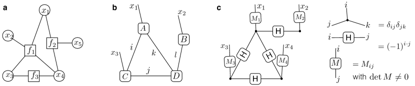
Figure 1: Classical and quantum generative models. a, Illustration of a factor graph, which includes widely-used classical generative models as its special cases. A factor graph is a bipartite graph where one group of the vertices represent variables (denoted by circles) and the other group of vertices represent positive functions (denoted by squares) acting on connected variables. The corresponding probability distribution is given by the product of all these functions. For instance, the probability distribution in (a) is $p(x_{1},x_{2},x_{3},x_{4},x_{5})=f_{1}(x_{1},x_{2},x_{3},x_{4})f_{2}(x_{1},x_{4},x_{5})f_{3}(x_{3},x_{4})/Z$ where $Z$ is a normalization factor. Each variable connects to at most a constant number of functions which introduce correlations in the probability distribution. b, Illustration of a tensor network state. Each unshared (shared) edge represents a physical (hidden) variable, and each vertex represents a complex function of the variables on its connected edges. The wave function of the physical variables is defined as a product of the functions on all the vertices, after summation (contraction) of the hidden variables. Note that a tensor network state can be regarded as a quantum version of the factor graph after partial contraction (similar to marginal probability in classical case) with positive real functions replaced by complex functions. c, Definition of a quantum generative model (QGM) introduced in this paper. The state is a special type of tensor network state, with the vertex functions fixed to be three types as shown on the right side. Without the single-qubit invertible matrix $M_{i}$ which contains the model parameters, the wave function connected by Hadamard and identity matrices just represent a graph state. To get a probability distribution from this model, we measure a subset of $n$ qubits (among total $m$ qubits corresponding to physical variables) in the computational basis under this state. The unmeasured $m-n$ qubits are traced over to get the marginal probability distribution $P(\{x_{i}\})$ of the measured $n$ qubits. We prove in this paper that the $P(\{x_{i}\})$ is general enough to include probability distributions of all classical factor graphs and special enough to allow a convenient quantum algorithm for the parameter training and inference.

In this paper, we propose a quantum algorithm with potential exponential speedup for machine learning based on generative models. Generative models are widely used to learn the underlying probability distribution describing correlations in observed data. It has utility in both supervised and unsupervised learning with a wide range of applications from classification, feature extraction, to creating new data such as style transfer shalev2014understanding ; goodfellow2016deep ; bishop2006pattern . Compared with discriminative models such as support vector machine or feed-forward neural network, generative models can express much more complex relations among variables jebara2012machine , which makes them broadly applicable but at the same time harder to tackle. Typical generative models include probabilistic graphical models such as Bayesian network and Markov random field bishop2006pattern , and generative neural networks such as Boltzmann machine and deep belief network. All these classical probabilistic models can be transformed into the so-called factor graphs bishop2006pattern .

Here we introduce a quantum generative model (QGM) where the probability distribution describing correlations in data is generated by measuring a set of observables under a many-body entangled state. A generative model is largely characterized by its representational power and its performance to learn the model parameters from the data and to make inference about complex relationship between any variables. In terms of representational power, we prove that our introduced QGM can efficiently represent any factor graphs, which include almost all the classical generative models in practical applications as particular cases. Furthermore, we show that the QGM is exponentially more powerful than factor graphs by proving that at least some instances generated by the QGM cannot be efficiently represented by any factor graph with polynomial number of variables if a widely accepted conjecture in computational complexity theory holds, that is, the polynomial hierarchy, which is a generalization of the famous P versus NP problem, does not collapse.

Representational power and generalization ability sm only measure one aspect of a generative model. On the other hand we need an effective algorithm for training and making inference. We propose a general learning algorithm utilizing quantum phase estimation of the constructed parent Hamiltonian for the underlying many-body entangled state. Although it is unreasonable to expect that the proposed quantum algorithm has polynomial scaling in runtime in all cases (as this implies ability of a quantum computer to efficiently solve any NP problem, an unlikely result), we prove that at least for some instances, our quantum algorithm has exponential speedup over any classical algorithm, assuming quantum computers cannot be efficiently simulated by classical computers, a conjecture which is believed to hold.

The intuition for quantum speedup in our algorithm can be understood as follows: the purpose of generative machine learning is to model any data generation process in nature by finding the underlying probability distribution. As nature is governed by the law of quantum mechanics, it is too restrictive to assume that the real world data can always be modelled by an underlying probability distribution as in classical generative models. Instead, in our quantum generative model, correlation in data is parameterized by the underlying probability amplitudes of a many-body entangled state. As the interference of quantum probability amplitudes can lead to phenomena much more complex than those from classical probabilistic models, it is possible to achieve big improvement in our quantum generative model under certain circumstances.

We start by defining factor graph and our QGM. Direct characterization of a probability distribution of $n$ binary variables has an exponential cost of $2^{n}$. A factor graph, which includes many classical generative models as special cases, is a compact way to represent $n$-particle correlation bishop2006pattern ; goodfellow2016deep . As shown in Fig. 1a, a factor graph is associated with a bipartite graph where the probability distribution can be expressed as a product of positive correlation functions of a constant number of variables. Here, without loss of generality, we assumed constant-degree graph, in which the maximum number of edges per vertex is bounded by a constant.

Our QGM is defined on a graph state $|G\rangle$ of $m$ qubits associated with a graph $G$. We introduce the following transformation

$$|Q\rangle\equiv M_{1}\otimes\cdots\otimes M_{m}|G\rangle,$$ (1)

where $M_{i}$ denotes an invertible (in general non unitary) $2\times 2$ matrix applied on the Hilbert space of qubit $i$. From $m$ vertices of the graph $G$, we choose a subset of $n$ qubits as the visible units and measure them in computational basis $\left\{\left|0\right\rangle,\left|1\right\rangle\right\}$. The measurement outcomes sample from a probability distribution $Q\left(\left\{x_{i}\right\}\right)$ of $n$ binary variables $\left\{x_{i},i=1,2,\cdots n\right\}$ (the other $m-n$ hidden qubits are just traced over to give the reduced density matrix). Given graph $G$ and the subset of visible vertices, the distribution $Q\left(\left\{x_{i}\right\}\right)$ defines our QGM which is parameterized efficiently by the parameters in the matrices $M_{i}$. The state $|Q\rangle$ can be written as a special tensor network state (see Fig. 1) sm . We define our model in this form for two reasons: first, the probability distribution $Q\left(\left\{x_{i}\right\}\right)$ needs to be general enough to include all factor graphs; second, if the state $|Q\rangle$ takes a specific form, the parameters in this model can be conveniently trained by a quantum algorithm on a data set.

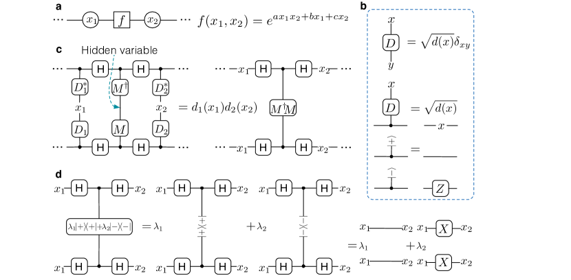
Figure 2: Efficient representation of factor graphs by the quantum generative model. a, The general form of correlation function of two binary variables in a factor graph, with parameters $a,b,c$ being real. This correlation acts as the building block for general correlations in any factor graph by use of the universal approximation theorem le2008representational . b, Notations of some common tensors and their identities: $D$ is a diagonal matrix with diagonal elements $\sqrt{d(x})$ with $x=0,1$; $Z$ is the diagonal Pauli matrix $\text{diag}(1,-1)$; and $|\pm\rangle=(|0\rangle\pm|1\rangle)/\sqrt{2}$. c, Representation of the building block correlator $f(x_{1},x_{2})$ in a factor graph (see a) by the QGM with one hidden variable (unmeasured) between two visible variables $x_{1},x_{2}$ (measured in the computational basis). We choose the single-bit matrix $D_{1},D_{2}$ to be diagonal with $D_{1}=\text{diag}(\sqrt{d_{1}(0)},\sqrt{d_{1}(1)})$ and $D_{2}=\text{diag}(\sqrt{d_{2}(0)},\sqrt{d_{2}(1)})$. In simplification of this graph, we used the identity in b. d, Further simplification of the graph in c, where we choose the form of the single-bit matrix $M^{{\dagger}}M$ acting on the hidden variable to be $M^{{\dagger}}M=\lambda_{1}|+\rangle\langle+|+\lambda_{2}|-\rangle\langle-|$ with positive eigenvalues $\lambda_{1},\lambda_{2}$. We used the identity in b and the relation $HZH=X$, where X (H) denotes the Pauli (Hadamard) matrix, respectively. By solving the values of $\lambda_{1},\lambda_{2},d_{1}(x_{1}),d_{2}(x_{2})$ in terms of $a,b,c$ (see the proof of Theorem 1), this correlator of QGM exactly reproduces the building block correlator $f(x_{1},x_{2})$ of the factor graph.

Now we show that any factor graph can be viewed as a special case of QGM by the following theorem:

Theorem 1.

The QGM defined above can efficiently represent probability distributions from any constant-degree factor graphs by an arbitrarily high precision.

As probabilistic graphical models and generative neural networks can all be reduced to constant-degree factor graphs bishop2006pattern ; sm , the above theorem shows that our proposed QGM is general enough to include those probability distributions in widely-used classical generative models.

Proof of Theorem 1: First, for any factor graph with degree bounded by a constant $k$, by the universal approximation theorem le2008representational , each $k$-variable node function can be approximated arbitrarily well with $2^{k}+k$ variables ($2^{k}$ of them are hidden) connected by the two-variable correlator that takes the generic form $f(x_{1},x_{2})=e^{ax_{1}x_{2}+bx_{1}+cx_{2}}$, where $x_{1}$, $x_{2}$ denote the binary variables and $a,b,c$ are real parameters. As $Q\left(\left\{x_{i}\right\}\right)$ has a similar factorization structure as the factor graph after measuring the visible qubits $x_{i}$ under a diagonal matrix $M_{i}$ (see Fig. 2), it is sufficient to show that each correlator $f(x_{1},x_{2})$ can be constructed in the QGM. This construction can be achieved by adding one hidden variable (qubit) $j$ with invertible matrix $M_{j}$ between two visible variables $x_{1}$ and $x_{2}$. As shown in Fig. 2, we take $M_{1}$ and $M_{2}$ to be diagonal with eigenvalues $\sqrt{d_{1}\left(x_{1}\right)}$ and $\sqrt{d_{2}\left(x_{2}\right)}$, respectively, and $M_{j}^{\dagger}M_{j}=\lambda_{1}\left|+\right\rangle\left\langle+\right|+\lambda_{2}\left|-\right\rangle\left\langle-\right|$, where $\left|\pm\right\rangle=\left(\left|0\right\rangle\pm\left|1\right\rangle\right)/\sqrt{2}$. The correlator between $x_{1}$ and $x_{2}$ in the QGM is then given by $d_{1}\left(x_{1}\right)d_{2}\left(x_{2}\right)\left[\lambda_{1}\delta_{x_{1}x_{2}}+\lambda_{2}(1-\delta_{x_{1}x_{2}})\right]/2$. We want it to be equal to $e^{ax_{1}x_{2}+bx_{1}+cx_{2}}$ to simulate the factor graph. There exists a simple solution with $d_{1}\left(0\right)=d_{2}\left(0\right)=\lambda_{1}/2=1$ and $d_{1}\left(1\right)=e^{b+a/2},$ $d_{2}\left(1\right)=e^{c+a/2},$ $\lambda_{2}=2e^{-a/2}$. This completes the proof.

Furthermore, we can show that the QGM is exponentially more powerful than factor graphs in representing probability distributions. This is summarized by the following theorem:

Theorem 2.

If the polynomial hierarchy in the computational complexity theory does not collapse, there exist probability distributions that can be efficiently represented by a QGM but cannot be efficiently represented even under approximation by conditional probabilities from any classical generative models that are reducible to factor graphs.

The proof of this theorem involves many terminologies and results from the computational complexity theory, so we present it in the Supplementary Material sm .

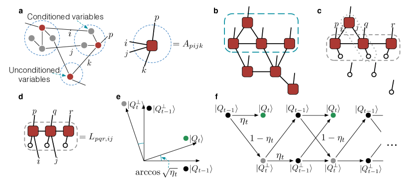
Figure 3: Illustration of our training algorithm for the quantum generative model. a, Training and inference of the QGM are reduced to measuring certain operators under the state $|Q(z)\rangle$. The key step of the quantum algorithm is therefore to prepare the state $|Q(z)\rangle$, which is achieved by recursive quantum phase estimation of the constructed parent Hamiltonian. The variables in the set $z$ whose values are specified are called conditioned variables, whereas the other variables that carry the binary physical index are called unconditioned variables. We group the variables in a way such that each group contains only one unconditioned variable and different groups are connected by a small constant number of edges (representing virtual indices or hidden variables). Each group then defines a tensor with one physical index (denoted by $p$) and a small constant number of virtual indices (denoted by $i,j,k$ in the figure). b, Tensor network representation of $|Q(z)\rangle$, where a local tensor is defined for each group specified in a. c, Tensor network representation of $|Q_{t}\rangle$, where $|Q_{t}\rangle$ are the series of states reduced from $|Q_{z}\rangle$. In each step of the reduction, one local tensor is moved out. The moved-out local tensors are represented by unfilled circles, each carrying a physical index set to $0$. For the edges between the remaining tensor network and the moved-out tensors, we set the corresponding virtual indices to $0$ (represented by unfilled circles). d, Construction of the parent Hamiltonian. The figure shows how to construct one term in the parent Hamiltonian, which corresponds to a group of neighboring local tensors such as those in the dashed box in c. After contraction of all virtual indices among the group, we get a tensor $L_{pqr,ij}$, which defines a linear map $L$ from virtual indices $i,j$ to physical indices $p,q,r$. As the indices $i,j$ take all the possible values, the range of this mapping $L$ spans a subspace $\text{range}(L)$ in the Hilbert space $H_{p,q,r}$ of the physical indices $p,q,r$. This subspace has a complementary orthogonal subspace inside $H_{p,q,r}$, denoted by $\text{comp}(L)$. The projector to the subspace $\text{comp}(L)$ then defines one term in the parent Hamiltonian, and by this definition $|Q_{t}\rangle$ lies in the kernel space of this projector. We construct each local term with a group of neighboring tensors. Each local tensor can be involved in several Hamiltonian terms (as illustrated in c by the dashed box and the dotted box), thus some neighboring groups have non-empty overlap, and they generate terms that in general do not commute. By this method, one can construct the parent Hamiltonian whose ground state uniquely defines the state $|Q_{t}\rangle$ perez2008peps . e, States involved in the evolution from $|Q_{t-1}\rangle$ to $|Q_{t}\rangle$ by quantum phase estimation applied on their parent Hamiltonians. $|Q_{t-1}^{\perp}\rangle,|Q_{t}^{\perp}\rangle$ represent the states orthogonal to $|Q_{t-1}\rangle,|Q_{t}\rangle$, respectively, inside the two-dimensional subspace spanned by $|Q_{t-1}\rangle$ and $|Q_{t}\rangle$. The angle between $|Q_{t}\rangle$ and $|Q_{t-1}\rangle$ is determined by the overlap $\eta_{t}=|\langle Q_{t}|Q_{t-1}\rangle|^{2}$. f, State evolution under recursive application of quantum phase estimation algorithm. Starting from the state $|Q_{t-1}\rangle$, we always stop at the state $|Q_{t}\rangle$, following any branch of this evolution, where $\eta_{t}$ and $1-\eta_{t}$ denote the probabilities of the corresponding outcomes.

For a generative model to be useful for machine learning, apart from high representational power and generalization ability (which are closely related sm ), we also need to have efficient algorithms for both inference and training. For inference, we usually need to compute conditional probability $\sum_{y}p(x,y|z)$ bishop2006pattern , where $x,y,z$ denote variable sets. For training, we choose to minimize the Kullback–Leibler (KL) divergence $D(q_{\text{d}}||p_{\theta})=-\sum_{v}q_{\text{d}}(v)\log(p_{\theta}(v)/q_{\text{d}}(v))$ between $q_{\text{d}}$, the distribution of the given data sample, and $p_{\theta}$, the distribution of the generative model, with the whole parameter set denoted by $\theta$. Typically, one minimizes $D(q_{\text{d}}||p_{\theta})$ by optimizing the model parameters $\theta$ using the gradient descent method goodfellow2016deep . The $\theta$-dependent part $D\left(\theta\right)$ of $D(q_{\text{d}}||p_{\theta})$ can be expressed as $-\sum_{v\in\text{data set}}\log p_{\theta}(v)/M$, where $M$ denotes the total number of data points. As the number of parameters is bounded by $\mbox{poly}(n)$, the required data size $M$ for training is typically also bounded by a $\mbox{poly}(n)$ function sm ; shalev2014understanding .

In our QGM, both of the conditional probability $\sum_{y}p(x,y|z)$ and the gradient of KL divergence $\partial_{\theta}D\left(\theta\right)$ can be conveniently calculated using the structure of state $|Q\rangle$ defined in Fig. 1. We first define a tensor network state $|Q(z)\rangle\equiv(I\otimes\langle z|)|Q\rangle$ by projecting the variable set $z$ to the computational basis. As shown in the Supplementary Material sm , the conditional probability can be expressed as

$$\sum_{y}p(x,y|z)=\frac{\langle Q(z)|O|Q(z)\rangle}{\langle Q(z)|Q(z)\rangle},$$ (2)

which is the expectation value of the operator $O=|x\rangle\langle x|$ under the state $|Q(z)\rangle$. Similarly, we show in the Supplementary Material sm that $\partial_{\theta}D\left(\theta\right)$ can be reduced to a combination of terms taking the same form as Eq. 2, with operator $O$ replaced by $O_{1}=(\partial_{\theta_{i}}M_{i})M_{i}^{-1}+H.c.$ or $O_{2}=|v_{i}\rangle\langle v_{i}|(\partial_{\theta_{i}}M_{i})M_{i}^{-1}+H.c.$, where $\theta_{i}$ denotes a specific parameter in the invertible matrix $M_{i}$; $v_{i}$ is the qubit of data $v$ corresponding to variable $x_{i}$; and $H.c.$ stands for the Hermitian conjugate term. The variable $z$ in this case takes the value of $v$ (or $v$ excluding $v_{i}$) expressed in a binary string.

With the above simplification, training or inference in the QGM is reduced to preparation of the tensor network state $|Q(z)\rangle$. With an algorithm similar to the one in Ref. schwarz2012preparing , we use recurrent quantum phase estimation to prepare the state $|Q(z)\rangle$. For this purpose, first we construct the parent Hamiltonian $H(z)$ whose unique ground state is $|Q(z)\rangle$. This is shown in Fig. 3, where the variables $z=\{z_{i}\}$ are grouped as in Fig. 3a. In this case, the corresponding local tensors in the tensor network state $|Q(z)\rangle$ are all easy to compute and of constant degree. The parent Hamiltonian $H(z)$ is constructed through contraction of these local tensors as shown in Fig. 3c to 3d perez2008peps .

By construction of the parent Hamiltonian for the tensor network state, the quantum algorithm for training and inference in the QGM is realized through the following steps:

Step 1: Construct a series of tensor network states $\{|Q_{t}\rangle\}$ with $t=0,1,...,n$ as shown in Fig. 3c by reduction from $|Q_{n}\rangle=|Q(z)\rangle$. The initial state $|Q_{0}\rangle$ is a product state $|0\rangle^{\otimes n}$, and $|Q_{t}\rangle$ is constructed from $|Q_{t-1}\rangle$ by adding one more tensor in $|Q(z)\rangle$ that is not contained in $|Q_{t-1}\rangle$ and setting the uncontracted virtual indices as $0$.

Step 2: Construct a parent Hamiltonian $H_{t}$ for each $|Q_{t}\rangle$ with the method illustrated in Fig. 3 perez2008peps .

Step 3: Starting from $|Q_{0}\rangle$, we prepare $|Q_{1}\rangle,...,|Q_{n}\rangle$ sequentially. Suppose we have prepared $|Q_{t-1}\rangle$, the following sub-steps will prepare $|Q_{t}\rangle$ based on the recursive quantum phase estimation.

Sub-step 1: Use the phase estimation algorithm abrams1999quantum on the parent Hamiltonians $H_{t}$ and $H_{t-1}$ to implement two projective measurements of $\{|Q_{t}\rangle\langle Q_{t}|,I-|Q_{t}\rangle\langle Q_{t}|\}$ and $\{|Q_{t-1}\rangle\langle Q_{t-1}|,I-|Q_{t-1}\rangle\langle Q_{t-1}|\}$ (see Fig. 3e). The runtime of this algorithm is proportional to $1/\Delta_{t}$ or $1/\Delta_{t-1}$ with some $\mbox{poly}(n)$ overhead, where $\Delta_{t}$ ($\Delta_{t-1}$) denotes the energy gap of the Hamiltonian $H_{t}$ ($H_{t-1}$).

Sub-step 2: Starting from $|Q_{t-1}\rangle$, we perform the projective measurement $\{|Q_{t}\rangle\langle Q_{t}|,I-|Q_{t}\rangle\langle Q_{t}|\}$. If the result is $|Q_{t}\rangle$, we succeed and skip the following sub-steps. Otherwise, we get $|Q_{t}^{\perp}\rangle$ lying in the plane spanned by $|Q_{t-1}\rangle$ and $|Q_{t}\rangle$.

Sub-step 3: We perform the projective measurement $\{|Q_{t-1}\rangle\langle Q_{t-1}|,I-|Q_{t-1}\rangle\langle Q_{t-1}|\}$ on the state $|Q_{t}^{\perp}\rangle$. The result is either $|Q_{t-1}\rangle$ or $|Q_{t-1}^{\perp}\rangle$.

Sub-step 4: We perform the projective measurement $\{|Q_{t}\rangle\langle Q_{t}|,I-|Q_{t}\rangle\langle Q_{t}|\}$ again. We either succeed in getting $|Q_{t}\rangle$, with probability $\eta_{t}=|\langle Q_{t}|Q_{t-1}\rangle|^{2}$, or have $|Q_{t}^{\perp}\rangle$. In the latter case, we go back to the sub-step 3 and continue until success.

The decision/evolution tree of the above process is shown in Fig. 3f. The computational time from $|Q_{t-1}\rangle$ to $|Q_{t}\rangle$ is proportional to the average number of sub-steps

$$\eta_{t}+\sum_{k=0}^{\infty}(4k+6)(1-\eta_{t})^{2}\eta_{t}(\eta_{t}^{2}+(1-\eta_{t})^{2})^{k}=\frac{1}{\eta_{t}}+1$$ (3)

Step 4: After successful preparation of the state $|Q(z)\rangle$, we measure the operator $O$ (for inference) or $O_{1}$, $O_{2}$ (for training), and the expectation value of the measurement gives the required conditional probability or the gradient of KL divergence for learning.

The runtime of the whole algorithm described above is proportional to the maximum of $1/\Delta_{t}$ and $1/\eta_{t}$. The gap $\Delta_{t}$ and the overlap $\eta_{t}$ depend on the topology of the graph $G$ and the parameters of the matrices $M_{i}$. If these two quantities are bounded by $\mbox{poly}(n)$ for all the steps $t$ from $1$ to $n$, this quantum algorithm will be efficient (runtime bounded by $\mbox{poly}(n)$). Although we do not expect this to be true in the worst case (even for the simplified classical generative model such as the restricted Boltzmann machine, the worst case complexity is at least NP hard dagum1993approximating ), we know that the QGM with the above heuristic algorithm will provide exponential speedup over classical generative models for some instances. In the Supplementary Material sm , we give a rigorous proof that our algorithm has exponential speedup over any classical algorithm for some instances under a reasonable conjecture. The major idea of this proof is as follows:

We construct a specific $|Q(z)\rangle$ which corresponds to the tensor network representation of the history state for universal quantum circuits rearranged into a two-dimensional (2D) spatial layout. The history state is a powerful tool in quantum complexity theory kitaev2002classical . Similar type of history state has been used before to prove the QMA-hardness for spin systems in a 2D lattice oliveira2008complexity . For this specific $|Q(z)\rangle$, we prove that both the gap $\Delta_{t}$ and the overlap $\eta_{t}$ scale as $1/\mbox{poly}(n)$ for all the steps $t$, by calculating the parent Hamiltonian of $|Q_{t}\rangle$ directly with proper grouping of local tensors. Our heuristic algorithm for training and inference therefore can be accomplished in polynomial time. On the other hand, our specific state $|Q(z)\rangle$ encodes universal quantum computation through representation of the history state, so it cannot be achieved by any classical algorithm in polynomial time if quantum computation cannot be efficiently simulated by a classical computer. We summarize the result with the following theorem:

Theorem 3.

There exist instances of computing conditional probability and gradient of KL divergence to additive error $1/\mbox{poly}(n)$ such that (i) our algorithm achieves it in polynomial time; (ii) any classical algorithm cannot accomplish them in polynomial time unless universal quantum computing can be simulated efficiently by a classical computer.

In summary, we have introduced a quantum generative model for machine learning and proven that it offers exponential improvement in representational power over widely-used classical generative models. We have also proposed a heuristic quantum algorithm for training and making inference on our model, and proven that this quantum algorithm offers exponential speedup over any classical algorithm at least for some instances if quantum computing cannot be efficiently simulated by a classical computer. Our result combines the tools of different areas and generates an intriguing link between quantum many-body physics, quantum computation and complexity theory, and the machine learning frontier. This result opens a new route to apply the power of quantum computation to solving the challenging problems in machine learning and artificial intelligence, which, apart from its fundamental interest, has wide application potential.

Acknowledgements This work was supported by the Ministry of Education and the National key Research and Development Program of China. LMD and ZYZ acknowledge in addition support from the MURI program.

Author Information All the authors contribute substantially to this work. The authors declare no competing financial interests. Correspondence and requests for materials should be addressed to L.M.D. (lmduanumich@gmail.com) or X. G. (gaoxungx@gmail.com).

Supplementary Material

In this supplementary information, we provide rigorous proofs of theorem 2 and theorem 3 in the main text. We also explain the relation between the representational power and the generational ability of a generative model, the reduction of typical classical generative models to factor graphs, and more details about the training and inference algorithms for our quantum generative model.

I Representational power and generalization ability

In this section, we briefly introduce some basic concepts in statistical learning theory vapnik2013natures , the theoretical foundation of machine learning. Then we discuss the intuitive connection between the generalization ability and representational power of a machine learning model. This connection does not hold in the sense of mathematical rigor and counter examples exist, however, it is still a good guiding principle in practice. More details can be found in the introductory book shalev2014understandings .

A simplified way to formulate a machine learning task is as follows: given $M$ data generated independently from a distribution $\mathcal{D}$ (which is unknown), a set of hypothesis $\mathcal{H}=\{h\}$ (which could be a model with some parameters) and a loss function $L$ characterizing how “good” a hypothesis $h$ is, try to find an $h_{A}$ produced by some machine learning algorithm $A$, minimizing the actual loss:

$$L_{\mathcal{D}}(h_{A})\sim\epsilon_{\text{bias}}+\epsilon_{\text{est}}\text{ where }\epsilon_{\text{bias}}=\min_{h\in\mathcal{H}}L_{\mathcal{D}}(h)\text{ and }\epsilon_{\text{est}}\text{ depends on }M.$$ (S1)

The term $\epsilon_{\text{bias}}$ represents the bias error. When $\mathcal{H}$ is a hypothesis class which is not rich enough or the number of parameters in the model is small, this term might be large no matter how many training data are given, which leads to underfitting. The term $\epsilon_{\text{est}}$ represents the generalization error. When $\mathcal{H}$ is a very rich hypothesis class or the number of parameters in the model is too large, this term might be large if the number of training data is not enough, which leads to overfitting. This is the bias-complexity trade-off of a machine learning model.

The generalization ability of a machine learning model is usually quantified by sample complexity $M(\epsilon_{\text{est}},\delta)$ in the framework of Probably Approximately Correct (PAC) learning valiant1984theorys , which means if the number of training data is larger than $M(\epsilon_{\text{est}},\delta)$, the generalization error is bounded by $\epsilon_{\text{est}}$ with probability at least $1-\delta$. It has been proved that the sample complexity has the same order of magnitude as a quantity of the hypothesis set $\mathcal{H}$, the Vapnik-Chervonenkis dimension (VC dimension)vapnik2015uniforms . The VC dimension could be used to characterize the “effective” degree of freedom of a model, which is the number of parameters in most situations. With a smaller VC dimension, the generalization ability gets better.

There are some caveats of using the VC dimension to connect the generalization ability and the representational power of a machine learning model though, which include: (i) the VC dimension theory only works in the framework of PAC learning (thus restricted to supervised learning), so it is not directly applicable to generative models; (ii) the number of parameters does not always match the VC dimension, e.g., the combination of several parameters as $\theta_{1}+\theta_{2}+\cdots$ only counts as one effective parameter, meanwhile there also exists such a model with only one parameter but having infinite VC dimensions. However, despite of existence of those counter examples, the VC dimension matches the number of parameters in most situations, so it is still a guiding principle to choose models with a smaller number of parameters. If the number of parameters is large, in order to determine each parameter, it needs a large amount of information, thus a large number of data is necessary.

In the case of the QGM, we find a distribution (illustrated by a blue circle in Fig. S1) such that, in order to represent it or equivalently make $\epsilon_{\text{bias}}$ small, the factor graph should have a number of parameters exponentially large (Fig. S1b). In this case, the distribution that the factor graph could represent has a very large degrees of freedom. However, the distribution which the QGM could represent only occupies a small corner of the whole distribution space (Fig. S1b), so the information needed to determine the parameters will be much smaller. Similar reasoning has been used to illustrate the necessity of using deep architecture in neural network goodfellow2016deeps ; maass1994comparisons ; maass1997boundss ; montufar2014numbers ; poggio2015theorys ; eldan2015powers ; mhaskar2016learning1s ; raghu2016expressives ; poole2016exponentials ; mhaskar2016learning2s ; lin2016doess ; liang2016deeps .

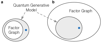
Figure S1: Parameter Space of Factor Graph and QGM. a, The case when both models have a polynomial number of parameters. In this case, factor graphs cannot represent some distributions in the QGM illustrated as blue circles. b, In order to represent the blue circle distribution from the QGM, factor graphs have to involve an exponentially large number of parameters. In this case, the parameter space will inflate to a very large scale.

II Reduction of typical generative models to factor graphs

In this section, we review typical classical generative models with graph structure. There are two large classes: one is the probabilistic graphical model koller2009probabilistics ; bishop2006patterns , and the other is the energy-based generative neural network. Strictly speaking, the later one is a special case of the former, but we regard it as another category because it is usually referred in the context of deep learning goodfellow2016deeps . We discuss the “canonical form” of generative models, the factor graph, and show how to convert various classical generative models into this canonical form. The details could be found in the books in Refs. koller2009probabilistics ; bishop2006patterns .

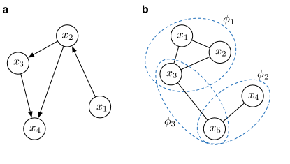
Figure S2: Probabilistic Graphical Models. a, The Bayesian network. The distribution defined by this figure is $P(x_{1},x_{2},x_{3},x_{4})=P(x_{1})P(x_{2}|x_{1})P(x_{3}|x_{2})P(x_{4}|x_{2},x_{3})$. b, Markov random field. The distribution defined by this figure is $P(x_{1},x_{2},x_{3},x_{4})=\phi_{1}(x_{1},x_{2},x_{3})\phi_{2}(x_{4},x_{5})\phi_{3}(x_{3},x_{5})/Z$ where $Z=\sum_{x_{1},x_{2},x_{3},x_{4}}P(x_{1},x_{2},x_{3},x_{4})$ is the normalization factor or partition function. Each dashed circle corresponds to a clique.

First, we introduce two probabilistic graphical models as shown in Fig. S2: the Bayesian network (directed graphical model) and the Markov random field (undirected graphical model). A Bayesian network (Fig. S2a) is defined on a directed acyclic graph. For each node $x_{i}$, assign a transition probability $P(x_{i}|\text{parents of }x_{i})$ where the parent means starting point of a directed edge of which the end point is $x_{i}$. If there is no parent for $x_{i}$, assign a probability $P(x_{i})$. The total probability distribution is the product of these conditional probabilities. A Markov random field (Fig. S2b) is defined on an undirected graph. The sub-graph in each dashed circle is a clique in which each pair of nodes is connected. For each clique, assign a non-negative function for each node variable. The total probability distribution is proportional to the product of these functions.

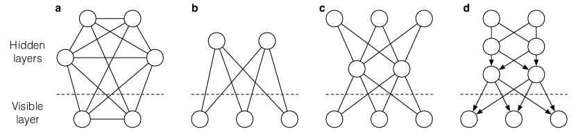
Figure S3: Energy-based Neural Networks. a, Boltzmann machine. A fully connected graph. The correlation between each pair $x_{i}$ and $x_{j}$ is $e^{ax_{i}x_{j}+bx_{i}+cx_{j}+d}$ with $a,b,c,d$ being real numbers. The whole distribution is proportional to the product of all the correlation between each pair of nodes, which is a Gibbs distribution with two-body interaction and classical Hamiltonians. b, Restricted Boltzmann Machine. Bipartite graph (graph with only two layers). The correlation is the same as in a except $a=b=c=d=0$ between the pairs not connected. There is no connection between pairs in the same layer. c, Deep Boltzmann machine. Basically the same as b except there are more than two hidden layers. d, Deep belief network. A mixture of undirected and directed graphical model. The top two layers define a restricted Boltzmann machine. For each node $y_{j}$ as the end point of directed edges, it is assigned a conditional probability $P(y_{j}=0|\cdots,x_{i},\cdots)=1/(1+e^{\sum_{i}a_{ij}x_{i}+b_{j}})$. The distribution of the variables in the visible layer is defined as the marginal probability.

Then we introduce four typical generative neural networks as shown in Fig. S3: the Boltzmann machine, the restricted Boltzmann machine, the deep Boltzmann machine, and the deep belief network. These neural networks are widely used in deep learning goodfellow2016deeps .

All the above generative models could be represented in the form of factor graph. Factor graph could be viewed as a canonical form of the generative models with graph structure. The factor graph representation of the Bayesian network and the Markov random field simply regards the conditional probability $P(x|y)$ and function $\phi(x,y)$ as the factor correlation $f(x,y)$. The factor graph representations of the Boltzmann machine, the restricted Boltzmann machine and the deep Boltzmann machine are graphs such that there is a square in each edge in the original network with correlation $f(x_{i},x_{j})=e^{ax_{i}x_{j}+bx_{i}+cx_{j}}$. The factor graph with unbounded degrees in these cases could be simulated by a factor graph with a constantly bounded degree, which is shown in Fig. S4. The idea is to add equality constraints which could be simulated by correlation $e^{ax_{i}x_{j}-ax_{i}/2-ax_{j}/2}$ with $a$ being a very large positive number since

$$e^{ax_{i}x_{j}-ax_{i}/2-ax_{j}/2}=\delta_{x_{i}x_{j}}+e^{-a/2}(1-\delta_{x_{i}x_{j}})\longrightarrow\delta_{x_{i}x_{j}}\text{ as }a\rightarrow+\infty.$$ (S2)

The factor graph representation of the deep belief network is a mixture of the Bayesian network and the restricted Boltzmann machine except that one correlation in the part of directed graph involves an unbounded number of variables. This is the conditional probability with one variable conditioned on the values of variables in the previous layer. It is

$$P(y|\cdots,x_{i},\cdots)=\frac{e^{(\sum_{i}a_{ij}x_{i}+b_{j})y}}{1+e^{\sum_{i}a_{ij}x_{i}+b_{j}}}.$$ (S3)

where $\{\cdots,x_{i},\cdots\}$ are the parents of $y$. Given the values of $\cdots,x_{i},\cdots$, it’s easy to sample $y$ according to $P(y|\cdots,x_{i},\cdots)$ (which is actually the original motivation for introducing the deep belief network). Thus the process could be represented by a Boolean circuit with random coins. In fact, a circuit with random coins is a Bayesian network: each logical gate is basically a conditional probability (for example, the AND gate $y=x_{1}\land x_{2}$ could be simulated by the conditional probability $P(y|x_{1}x_{2})=\delta_{y,x_{1}\cdot x_{2}}$). So this conditional probability could be represented by a Bayesian network in which the degree of each node is bounded by a constant. Thus deep belief network could be represented by a factor graph with a constant degree.

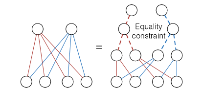
Figure S4: Simulating graphs of unbounded degrees with graphs of constantly bounded degrees. In the case that all the correlations involve only two variables (e.g., for Boltzmann machines), the correlation between one node and $l$ other nodes could be simulated by a binary tree structure with depth $\log l$. The newly added nodes and connections are marked by the dashed circles and lines, respectively. The correlation in the dashed line is an equality constraint which could be approximated by $e^{ax_{i}x_{j}-ax_{i}/2-ax_{j}/2}$ with $a$ being a very large positive number.

One important property is that the conditional probability of a factor graph is still factor graph. Actually, the correlation becomes simpler: the number of variables involved does not increase, which means approximately computing the conditional probability of probabilistic graphical models could be reduced to preparing the state $|Q\rangle$ (which will be shown in next section ). Then we arrive at the following lemma:

Lemma 1.

 All the probability distributions or conditional probability distributions of probabilistic graphical models and energy-based neural networks can be represented efficiently by the factor graph with a constant degree.

III Parent Hamiltonian of the State $|Q\rangle$

We consider tensor network representation of $|Q\rangle$ defined on a graph with a constant degree.

$$|Q\rangle\equiv M_{1}\otimes\cdots\otimes M_{n}|G\rangle$$ (S4)

where $|G\rangle$ is the graph state that is the unique ground state of the frustration-free local Hamiltonian with zero ground-state energy:

$$H_{G}=\sum_{i}H_{i}=\sum_{i}\frac{I-\left(\bigotimes_{j\in\{i\text{'s neighbors}\}}Z_{j}\right)\otimes X_{i}}{2}$$ (S5)

where each $H_{i}$ is the projector of the stabilizer gottesman1997stabilizers ; raussendorf2001ones supported only on the node $i$ and its neighbors, thus being local since the degree of the graph is a constant. And

$$H_{i}|G\rangle=0.$$ (S6)

Next we construct a Hamiltonian:

$$H_{Q}=\sum_{i}H_{i}^{\prime}=\sum_{i}\left(\bigotimes_{j\in\{i\}\cup\{i\text{'s neighbors}\}}M_{j}^{-1}\right)^{{\dagger}}H_{i}\left(\bigotimes_{j\in\{i\}\cup\{i\text{'s neighbors}\}}M_{j}^{-1}\right).$$ (S7)

First, we show that $|Q\rangle$ is the ground state of $H_{Q}$. Since $H_{i}$ is positive semidefinite, thus $H_{i}^{\prime}$ is also positive semidefinite, the eigenvalue of $H_{Q}$ is no less than $0$.

$$\langle Q|H_{i}^{\prime}|Q\rangle = \langle Q|\left(\bigotimes_{j\in\{i\}\cup\{i\text{'s neighbors}\}}M_{j}^{-1}\right)^{{\dagger}}H_{i}\left(\bigotimes_{j\in\{i\}\cup\{i\text{'s neighbors}\}}M_{j}^{-1}\right)|Q\rangle$$ (S8)

$$= \langle G|\left(\bigotimes_{k\in\text{all the nodes except for }j\text{s}}(M_{k}M_{k}^{{\dagger}})^{-1}\right)\otimes H_{i}|G\rangle$$

$$= 0,$$

so $\langle Q|H_{Q}|Q\rangle=0$ which means $|Q\rangle$ is the ground state of $H_{Q}$. Then we prove $|Q\rangle$ is the unique ground state. Suppose $|Q^{\prime}\rangle=M_{1}\otimes\cdots\otimes M_{n}|G^{\prime}\rangle$ satisfying $\langle Q^{\prime}|H_{Q}|Q^{\prime}\rangle=0$ for some state $|G^{\prime}\rangle$, which implies $\langle Q^{\prime}|H_{i}^{\prime}|Q^{\prime}\rangle=0$ for every $i$. So

$$\langle Q^{\prime}|H_{i}^{\prime}|Q^{\prime}\rangle = \langle Q^{\prime}|\left(\bigotimes_{j\in\{i\}\cup\{i\text{'s neighbors}\}}M_{j}^{-1}\right)^{{\dagger}}H_{i}\left(\bigotimes_{j\in\{i\}\cup\{i\text{'s neighbors}\}}M_{j}^{-1}\right)|Q^{\prime}\rangle$$ (S9)

$$= \langle G^{\prime}|H_{i}\otimes\left(\bigotimes_{k\in\text{all the nodes except for }j\text{s}}(M_{k}M_{k}^{{\dagger}})^{-1}\right)|G^{\prime}\rangle$$

$$= \left|H_{i}\otimes\left(\bigotimes_{k\in\text{all the nodes except for }j\text{s}}M_{k}^{-1}\right)|G^{\prime}\rangle\right|_{2}$$

$$= 0,$$

which implies

$$H_{i}\otimes\left(\bigotimes_{k\in\text{all the nodes except for }i\text{ and }j\text{s}}M_{k}^{-1}\right)|G^{\prime}\rangle=0\Longrightarrow H_{i}|G^{\prime}\rangle=0$$ (S10)

for every $i$, thus $|G\rangle=|G^{\prime}\rangle$. This proves the uniqueness of $|Q\rangle$ as the ground state of $H_{Q}$.

IV Proof of Theorem 2

In this section, we use computational complexity theory to prove the exponential improvement on representational power of the QGM over any factor graph in which each correlation is easy to compute given a specific value for all variables (including all the models mentioned above). The discussion of the relevant computational complexity theory could be found in the book in Ref. arora2009computationals or in the recent review article on quantum supremacy Harrow2017s .

To prove theorem 2, first we define the concept of multiplicative error. Denote the probability distribution produced by the QGM as $\{q(x)\}$. Then we ask whether there exists a factor graph such that its distribution $\{p(x)\}$ approximates $\{q(x)\}$ to some error. It is natural to require that if $q(x)$ is very small, $p(x)$ should also be very small, which means rare events should still be rare. So we define the following error model:

Definition 1 (Multiplicative Error).

 Distribution $\{p(x)\}$ approximates distribution $\{q(x)\}$ to multiplicative error means

$$|p(x)-q(x)|\leq\gamma q(x)$$ (S11)

for any $x$, where $\gamma=\Omega(1/\mbox{poly}(n))<1/2$.

This error can also guarantee that any local behavior is approximately the same since the $l_{1}$-distance can be bounded by it:

$$\sum_{x}|p(x)-q(x)|\leq\sum_{x}\gamma q(x)=\gamma.$$ (S12)

But only bounding $l_{1}$-distance cannot guarantee that rare event is still rare. Multiplicative error for small $\gamma$ implies that the KL-divergence is bounded by

$$\left|\sum_{x}q(x)\log\frac{p(x)}{q(x)}\right| \leq \sum_{x}q(x)\log\left(1+\left|\frac{p(x)}{q(x)}-1\right|\right)$$ (S13)

$$\leq \sum_{x}q(x)\gamma=\gamma.$$

The probability $p(x|z)$ of a factor graph can be written as

$$p(x|z)=\frac{\sum_{y}p(x,y,z)}{\sum_{x,y}p(x,y,z)}=\frac{\sum_{y}f(x,y)}{\sum_{x,y}f(x,y)}$$ (S14)

where $f(x,y)$ is product of a polynomial number of relatively simple correlations, thus non-negative and can be computed in polynomial time and $y$ are hidden variables.

The probability $q(x)$ of the QGM can be written as

$$q(x)=\frac{\sum_{y}g(x,y)}{\sum_{x,y}g(x,y)}$$ (S15)

where $g(x,y)$ is product of a polynomial number of tensors given a specific assignment of indices and $y$ are the virtual indices or physical indices of hidden variables, $x$ is the remaining physical indices. Different from $f(x,y)$, $g(x,y)$ is a complex number in general. Thus in some sense, we can say $q(x)$ is the result of quantum interference in contrast to the case of $p(x)$ (or $p(x|z)$) which is only summation of non-negative numbers. Since $q(x)$ is summation of complex numbers, in the process of summation, it can oscillate dramatically, so we expect $q(x)$ being more complex than $p(x)$ (or $p(x|z)$). This can be formalized as the following lemma.

Lemma 2 (Stockmeyer’s theorem stockmeyer1976polynomials ).

 There exists an $\mathsf{FBPP}^{\mathsf{NP}}$ algorithm which can approximate

$$P=\Pr_{t}[f(t)=1]=\frac{1}{2^{r}}\sum_{t\in\{0,1\}^{r}}f(t)$$ (S16)

by $\widetilde{P}$, for any boolean function $f:\{0,1\}^{r}\rightarrow\mathbb{R}^{+}\cup\{0\}$, to multiplicative error $|\widetilde{P}-P|\leq P/\mbox{poly}(n)$ if $f(t)$ can be computed efficiently given $t$.

$\mathsf{FBPP}^{\mathsf{NP}}$ algorithms denote algorithms that a probabilistic Turing machine, supplied with an oracle that can solve all the NP problems in one step, can run in polynomial time.

Without the constraint $f(t)\geq 0$, approximating $P$ by $\widetilde{P}$ such that $|P-\widetilde{P}|\leq\gamma P$ is in general #P-hard even if $\gamma<1/2$. Roughly speaking, the complexity class #P valiant1979complexitys includes problems counting the number of witnesses of an NP problem, which is believed much harder than NP (see Ref. Harrow2017s for a quantum computing oriented introduction). The above lemma shows that summation of non-negative numbers is easier than complex numbers in general. This formulates that quantum interference is more complex than classical probability superposition.

Stockmeyer’s theorem was firstly used to separate classical and quantum distribution in Ref. aaronson2011computationals where the classical distribution is sampled by a probabilistic Turing machine in polynomial time and the quantum distribution is sampled from linear optics network. In some sense, our result could be viewed as a development of this result: the classical distribution is not necessarily sampled by a classical device efficiently, instead, the distribution could be approximated by a factor graph to multiplicative error. An efficient classical device is a special case of factor graph because it could be represented as a Boolean circuit with random coins, this could be represented as the Bayesian network as we have discussed above about the representation of deep belief network by factor graph.

Then we give the proof of theorem 2:

Proof.

Assume there exists a factor graph from which we can compute the conditional probability $p(x|z)$, we will prove that approximating $q(x)$ to multiplicative error, i.e., $|p(x|z)-q(x)|\leq\gamma q(x)$, is in $\mathsf{FBPP}^{\mathsf{NP}}/\mbox{poly}$ (the meaning of this complexity class will be explained later).

Suppose $f$ is defined as $p(x,y|z)$, there exists an $\mathsf{FBPP}^{\mathsf{NP}}$ algorithm approximating $P_{1}=\sum_{x,y}f(x,y)$ by $\widetilde{P}_{1}$ such that $|P_{1}-\widetilde{P}_{1}|\leq\gamma_{1}P_{1}$ and $P_{2}=\sum_{y}f(x,y)$ by $\widetilde{P}_{2}$ such that $|P_{2}-\widetilde{P}_{2}|\leq\gamma_{2}P_{2}$. Define $\widetilde{p}(x)=\widetilde{P}_{2}/\widetilde{P}_{1}$ and we have $p(x|z)=P_{2}/P_{1}$

$$|\widetilde{p}(x)-p(x|z)| = \left|\frac{\widetilde{P}_{2}}{\widetilde{P}_{1}}-\frac{P_{2}}{P_{1}}\right|$$ (S17)

$$\leq \left|\frac{\widetilde{P}_{2}}{\widetilde{P}_{1}}-\frac{P_{2}}{\widetilde{P}_{1}}\right|+\left|\frac{P_{2}}{\widetilde{P}_{1}}-\frac{P_{2}}{P_{1}}\right|$$

$$= \frac{|\widetilde{P}_{2}-P_{2}|}{\widetilde{P}_{1}}+P_{2}\left|\frac{1}{\widetilde{P}_{1}}-\frac{1}{P_{1}}\right|$$

$$= \frac{|\widetilde{P}_{2}-P_{2}|}{\widetilde{P}_{1}}+\frac{P_{2}}{\widetilde{P}_{1}P_{1}}|\widetilde{P}_{1}-P_{1}|$$

$$\leq (\gamma_{1}+\gamma_{2})\frac{P_{2}}{\widetilde{P}_{1}}$$

$$\leq \frac{\gamma_{1}+\gamma_{2}}{1-\gamma_{1}}\frac{P_{2}}{P_{1}}$$

$$= \frac{\gamma_{1}+\gamma_{2}}{1-\gamma_{1}}p(x|z),$$

then

$$|\widetilde{p}(x)-q(x)|\leq|\widetilde{p}(x)-p(x|z)|+|p(x|z)-q(x)|\leq\frac{\gamma_{1}+\gamma_{2}}{1-\gamma_{1}}p(x|z)+\gamma q(x)\leq\frac{\gamma+\gamma_{1}+\gamma_{2}+\gamma_{2}\gamma}{1-\gamma_{1}}q(x)<\frac{1}{2}q(x),$$ (S18)

the last step is because we choose $\gamma_{1}$ and $\gamma_{2}$ as sufficiently small as $1/\mbox{poly}(n)$. Under the assumption that the representation is efficient, such $f(x,y)$ can be represented by a polynomial size circuit, where the circuit corresponds to the description of the factor graph. So $\widetilde{p}(x)$ can be computed in $\mathsf{FBPP}^{\mathsf{NP}}/\mbox{poly}$. “/poly” is because we do not need to construct the circuit efficiently karp1982turings .

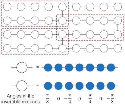
Figure S5: #P-hardness for QGM. The state $|Q\rangle$ in Ref. gao2016quantums . To construct this state, we start from a brickwork of white circles broadbent2009universals (the top side), with each white circle representing seven blue circles. Each blue circle represents a qubit. Then we apply $HZ(\theta)$ which is clearly an invertible matrix on each qubit with the angle $\theta$ shown at the bottom.

In Ref. gao2016quantums , we introduced a special form of QGM that corresponds to a graph state $|Q\rangle$ (Fig. S5) with one layer of invertible matrices $HZ(\theta)$ such that computing $q(x)$ to multiplicative error with $\gamma<1/2$ is at least $\mathsf{FP}^{\mathsf{\#P}}$. So assuming the efficient representation of QGM by factor graph, we will get

$$\mathsf{P}^{\mathsf{\#P}}\subseteq\mathsf{BPP}^{\mathsf{NP}}/\mbox{poly}.$$ (S19)

Then it follows basically the same reasoning as the proof of theorem 3 in Ref. aaronson2017implausibilitys except they consider $\mathsf{P}^{\mathsf{\#P}}\subseteq\mathsf{BPP}^{\mathsf{NP}^{\mathsf{NP}}}/\mbox{poly}$ and the result is polynomial hierarchy collapse to the fourth level. According to Toda’s theorem toda1989computationals , PH$\subseteq\mathsf{P}^{\mathsf{\#P}}$, this implies $\mathsf{NP}^{\mathsf{NP}}\subseteq\mathsf{BPP}^{\mathsf{NP}}/\mbox{poly}$. According to Adleman’s result adleman1978twos , BPP$\subseteq$P/poly, relativizes, which means $\mathsf{NP}^{\mathsf{NP}}\subseteq\mathsf{P}^{\mathsf{NP}}/\mbox{poly}$. Karp-Lipton theorem karp1982turings states if $\textsf{NP}\subset\textsf{P}/\mbox{poly}$, then $\Sigma^{p}_{2}\subseteq\Pi^{p}_{2}$ (polynomial hierarchy collapse to the second level); the result is also relativizing then it follows if $\mathsf{NP}^{\mathsf{NP}}\subseteq\mathsf{P}^{\mathsf{NP}}/\mbox{poly}$, then ${\Sigma^{p}_{2}}^{\textsf{NP}}\subseteq{\Pi^{p}_{2}}^{\textsf{NP}}$ which means $\Sigma^{p}_{3}\subseteq\Pi^{p}_{3}$ (polynomial hierarchy collapse to the third level). ∎

V Training and inference in quantum generative model

In this section, we discuss how to train the QGM and make inference on it. First, we briefly review how to train and make inference on some typical factor graphs. Then we reduce inference on the QGM to preparation of a tensor network state. Finally, we derive the formula for computing gradient of the KL-divergence of QGM and reduce it to the preparation of a tensor network state.

Inference problems on probabilistic graphical models include computing marginal probability $\sum_{y}p(x,y)$ and conditional probability $\sum_{y}p(x,y|z)$ (which includes marginal probability as a special case when the set $z$ is empty). To approximately compute the probability on some variables, we sample the marginal probability $p(x,y)$ or the conditional probability $p(x,y|z)$, and then measure the variable set $x$. We use the Boltzmann machine as an example to show how to train energy-based neural networks. The KL-divergence given $M$ data is

$$\frac{1}{M}\sum_{v\in\text{data set}}\log p(v).$$ (S20)

The training is to optimize this quantity with the gradient descent method. The gradient (for simplicity, we only present $\partial_{a}$ between hidden and visible nodes) is

$$\frac{1}{M}\partial_{a_{ij}}\sum_{v\in\text{data set}}\log p(v) = \frac{1}{M}\sum_{v\in\text{data set}}\sum_{h}P(h|v)h_{i}v_{j}-\sum_{h,v}P(h,v)h_{i}v_{j}$$ (S21)

$$= \langle h_{i}v_{j}\rangle_{\text{data}}-\langle h_{i}v_{j}\rangle_{\text{model}}.$$

The subscript “data” denotes distribution with probability $1/M$ randomly chosen from the training data according to $P(h|v)=P(h,v)/P(v)$, where $P(h,v)$ is the distribution defined by the graphical model, randomly sampling hidden variables $h$. The distribution “model” is $P(h,v)$. So the training is reduced to sampling some distribution or conditional distribution defined by the generative neural network and then estimating the expectation value of local observables. Since the QGM could represent conditional probability of these models and the corresponding state $|Q\rangle$ is the unique ground state of local Hamiltonian, inference and training could be reduced to the ground state preparation problem.

Similarly, inference on the QGM could also be reduced to preparation of a quantum state. As an example, let us compute the marginal probability for the QGM:

$$q(x)=\sum_{y}q(x,y)=\sum_{y}\frac{\langle Q|x,y\rangle\langle x,y|Q\rangle}{\langle Q|Q\rangle}=\frac{\langle Q|(|x\rangle\langle x|\otimes I)|Q\rangle}{\langle Q|Q\rangle}=\frac{\langle Q|(O\otimes I)|Q\rangle}{\langle Q|Q\rangle}.$$ (S22)

So the problem is reduced to preparing the state $|Q\rangle$ and then measuring the local observable $O$. Similarly, the conditional probability is given by

$$q(x|z)=\sum_{y}\frac{q(x,y,z)}{q(z)}=\frac{\langle Q(z)|(|x\rangle\langle x|\otimes I)|Q(z)\rangle}{\langle Q(z)|Q(z)\rangle}=\frac{\langle Q(z)|(O\otimes I)|Q(z)\rangle}{\langle Q(z)|Q(z)\rangle},$$ (S23)

where

$$|Q(z)\rangle\equiv(I\otimes\langle z|)|Q\rangle$$ (S24)

is a tensor network state.

The KL-divergence of the QGM is given by

$$\frac{1}{M}\sum_{v\in\text{data set}}\log{\langle Q(v)|Q(v)\rangle}-\log\langle Q|Q\rangle,$$ (S25)

and its derivative with respect to a parameter $\theta_{i}$ in $M_{i}$ is

$$\partial_{\theta_{i}}\left(\frac{1}{M}\sum_{v\in\text{data set}}\log{\langle Q(v)|Q(v)\rangle}-\log\langle Q|Q\rangle\right) = \frac{1}{M}\sum_{v\in\text{data set}}\frac{\partial_{\theta_{i}}\langle Q(v)|Q(v)\rangle}{\langle Q(v)|Q(v)\rangle}-\frac{\partial_{\theta_{i}}\langle Q|Q\rangle}{\langle Q|Q\rangle}.$$ (S26)

Let us consider the second term first.

$$\frac{\partial_{\theta_{i}}\langle Q|Q\rangle}{\langle Q|Q\rangle} = \frac{\partial_{\theta_{i}}\langle G|M_{1}^{\dagger}M_{1}\otimes\cdots\otimes M_{n}^{\dagger}M_{n}|G\rangle}{\langle Q|Q\rangle}$$ (S27)

$$= \frac{\langle G|M_{1}^{\dagger}M_{1}\otimes\cdots\otimes\partial_{\theta_{i}}M_{i}^{\dagger}M_{i}\otimes\cdots\otimes M_{n}^{\dagger}M_{n}|G\rangle}{\langle Q|Q\rangle}$$

$$= \frac{\langle G|M_{1}^{\dagger}M_{1}\otimes\cdots\otimes\left(M_{i}^{\dagger}(\partial_{\theta_{i}}M_{i})+(\partial_{\theta_{i}}M_{i}^{\dagger})M_{i}\right)\otimes\cdots\otimes M_{n}^{\dagger}M_{n}|G\rangle}{\langle Q|Q\rangle}$$

$$= \frac{\langle G|M_{1}^{\dagger}M_{1}\otimes\cdots\otimes\left(M_{i}^{\dagger}(\partial_{\theta_{i}}M_{i})M_{i}^{-1}M_{i}+M_{i}^{\dagger}M_{i}^{{\dagger}-1}(\partial_{\theta_{i}}M_{i}^{\dagger})M_{i}\right)\otimes\cdots\otimes M_{n}^{\dagger}M_{n}|G\rangle}{\langle Q|Q\rangle}$$

$$= \frac{\langle Q|(\partial_{\theta_{i}}M_{i})M_{i}^{-1}+M_{i}^{{\dagger}-1}(\partial_{\theta_{i}}M_{i}^{\dagger})|Q\rangle}{\langle Q|Q\rangle}.$$

It is basically the same for $|Q(v)\rangle$ if $\theta_{i}$ is the parameter for the unconditioned qubit:

$$\frac{\partial_{\theta_{i}}\langle Q(v)|Q(v)\rangle}{\langle Q(v)|Q(v)\rangle}=\frac{\langle Q(v)|(\partial_{\theta_{i}}M_{i})M_{i}^{-1}+M_{i}^{{\dagger}-1}(\partial_{\theta_{i}}M_{i}^{\dagger})|Q(v)\rangle}{\langle Q(v)|Q(v)\rangle}.$$ (S28)

If $\theta_{i}$ is the parameter of conditioned variables, it is more complicated. Let $|R_{i}\rangle=M_{i}^{-1}(I\otimes\langle v/v_{i}|)|Q(v)\rangle$ which is independent of $\theta_{i}$ and $(I\otimes\langle v_{i}|M_{i})|R_{i}\rangle=|Q(v)\rangle$, $(I\otimes M_{i})|R_{i}\rangle=|Q(v/v_{i})\rangle$, where $v/v_{i}$ denote all variables in $v$ except $v_{i}$.

$$\frac{\partial_{\theta_{i}}\langle Q(v)|Q(v)\rangle}{\langle Q(v)|Q(v)\rangle} = \frac{\langle R_{i}|\partial_{\theta_{i}}(M_{i}^{\dagger}|v_{i}\rangle\langle v_{i}|M_{i})|R_{i}\rangle}{\langle Q(v)|Q(v)\rangle}$$ (S29)

$$= \frac{\langle R_{i}|(\partial_{\theta_{i}}M_{i}^{\dagger})|v_{i}\rangle\langle v_{i}|M_{i}+M_{i}^{\dagger}|v_{i}\rangle\langle v_{i}|(\partial_{\theta_{i}}M_{i})|R_{i}\rangle}{\langle Q(v)|Q(v)\rangle}$$

$$= \frac{\langle R_{i}|M_{i}^{\dagger}M_{i}^{{\dagger}-1}(\partial_{\theta_{i}}M_{i}^{\dagger})|v_{i}\rangle\langle v_{i}|M_{i}+M_{i}^{\dagger}|v_{i}\rangle\langle v_{i}|(\partial_{\theta_{i}}M_{i})M_{i}^{-1}M_{i}|R_{i}\rangle}{\langle Q(v)|Q(v)\rangle}$$

$$= \frac{\langle Q(v/v_{i})|M_{i}^{{\dagger}-1}(\partial_{\theta_{i}}M_{i}^{\dagger})|v_{i}\rangle\langle v_{i}|+|v_{i}\rangle\langle v_{i}|(\partial_{\theta_{i}}M_{i})M_{i}^{-1}|Q(v/v_{i})\rangle}{\langle Q(v)|Q(v)\rangle}$$

$$= \frac{\langle Q(v/v_{i})|M_{i}^{{\dagger}-1}(\partial_{\theta_{i}}M_{i}^{\dagger})|v_{i}\rangle\langle v_{i}|+|v_{i}\rangle\langle v_{i}|(\partial_{\theta_{i}}M_{i})M_{i}^{-1}|Q(v/v_{i})\rangle}{\langle Q(v/v_{i})|Q(v/v_{i})\rangle}/\frac{\langle Q(v)|Q(v)\rangle}{\langle Q(v/v_{i})|Q(v/v_{i})\rangle}$$

$$= \frac{\langle Q(v/v_{i})|M_{i}^{{\dagger}-1}(\partial_{\theta_{i}}M_{i}^{\dagger})|v_{i}\rangle\langle v_{i}|+|v_{i}\rangle\langle v_{i}|(\partial_{\theta_{i}}M_{i})M_{i}^{-1}|Q(v/v_{i})\rangle}{\langle Q(v/v_{i})|Q(v/v_{i})\rangle}/\frac{\langle Q(v/v_{i})|v_{i}\rangle\langle v_{i}|Q(v/v_{i})\rangle}{\langle Q(v/v_{i})|Q(v/v_{i})\rangle}.$$

So computing gradient of KL-divergence of QGM reduces to preparing tensor network state $|Q(z)\rangle$ ($z$ being empty, $v$ or $v/v_{i}$ respectively) and measuring the expectation value of $O=|v\rangle\langle v|$, $O_{1}=(\partial_{\theta_{i}}M_{i})M_{i}^{-1}+c.c.$ and $O_{2}=|v_{i}\rangle\langle v_{i}|(\partial_{\theta_{i}}M_{i})M_{i}^{-1}+c.c.$. If the denominator is small, the error of the estimation through sampling could be large, in particular when the denominator is exponentially close to $0$. But we do not need to be pessimistic. Since this denominator represents the probability of getting $v_{i}$ for measuring the $i$-th variable, conditioned on the remaining variables being $v/v_{i}$, this quantity should not be small if the model distribution is close to the real data distribution. Otherwise, we are not able to observe this data. If the model distribution is far from the real data distribution, there is no need to estimate the gradient precisely. Moreover, statistical fluctuation in sampling in this case could even help to jump out of the local minimum, which is analogous to the stochastic gradient descent method in traditional machine learning shalev2014understandings ; goodfellow2016deeps .

The efficiency of estimating the expectation value of local observable through sampling depends on the maximum value of the observable. In the case of calculation of gradient of the KL-divergence, the maximum value depends on $M_{i}$ whose minimum singular value is set to $1$. Thus, the number of sampling is bounded by $\kappa^{2}/\epsilon^{2}$, where $\kappa$ is the condition number which is the maximum singular value of $M_{i}$, $\epsilon$ is the error of the estimation. In the case when $\kappa$ is large, $M_{i}$ is ill-conditioned, resulting in bad estimation. One strategy to avoid this situation is to use regularization term shalev2014understandings ; goodfellow2016deeps . For example, we may use

$$\sum_{i}\mbox{tr}M_{i}^{\dagger}M_{i}-\chi|\det M_{i}|^{2},$$ (S30)

as a penalty where $\chi>0$ is a hyperparameter which adjust the importance of the second term. The first term guarantees the singular value of $M_{i}$ should not be large and the second term guarantees that $\lambda_{1}\lambda_{2}$ should not be too small. In the case that $\max(\lambda_{1},\lambda_{2})$ is not too large, it guarantees that $\min(\lambda_{1},\lambda_{2})$ is not too small, which means $M_{i}$ is not too ill-conditioned.

VI Proof of Theorem 3

First, we prove that $|Q(z)\rangle$ could represent any tensor network efficiently:

Lemma 3.

Choosing the conditioned variables $z$ and invertible matrices properly, $|Q(z)\rangle$ could efficiently represent any tensor network in which each tensor has constant degree and the virtual index range is bounded by a constant.

Proof.

For a tensor $A_{i\cdots j}$, consider a quantum circuit preparing the following state:

$$\sum_{i\cdots j}A_{i\cdots j}|i\cdots j\rangle$$ (S31)

where the dimension of the Hilbert space is bounded by a constant if the number of indices and the range of each index of this tensor are bounded. The quantum circuit could be represented by a state $|Q(z)\rangle$ like the one in Fig. S5 with constant size, conditioned on specific values of some variables. This is just a post-selection of measurement result in measurement-based quantum computingraussendorf2001ones . Then we consider contracting virtual indices between different tensors. In this case, direct contraction will lead to a problem: the edge connecting two different tensors may be an identity tensor instead of a Hadamard tensor as in state $|Q\rangle$. We can solve this problem by introducing an extra variable in the middle of these two indices and connecting the two indices by Hadamard tensor. Further applying a Hadamard gate on it and conditioning on this extra variable being $0$, the net effect is equivalent to connecting the two indices by an identity tensor.∎

Since computation on the QGM is reduced to preparing $|Q(z)\rangle$, we will focus on tensor network construction for the state $|Q(z)\rangle$ in the following discussion. For an instance that our algorithm could run in polynomial time, $\min_{t}\Delta_{t}$ and $\min_{t}\eta_{t}$ should be both at least $1/\mbox{poly}(n)$. We construct a tensor network satisfying this requirement which at the same time encodes universal quantum computing. Therefore, a classical model is not able to to produce this result if quantum computation can not be efficiently simulated classically.

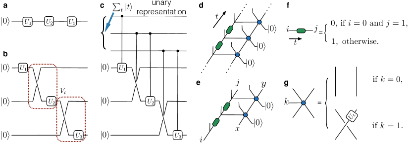
Figure S6: Construction of the History State. Illustration features one qubit only for convenience of drawing. It is straightforward to generalize it to the case of $n$ qubits by considering the layout of the circuits in Fig. 1 of Ref.oliveira2008complexitys . a, The universal quantum circuit. b, By adding swap gates and ancilla qubits, we can simulate the circuit in a by a 1D (2D for $n$ qubits case) tensor network state since there is only two gates applying on each qubit. The circuit in red dashed box is $V_{t}$. c, The history state of circuit b (here we omit the starting $|1\rangle$ and the end $|0\rangle$). d, Tensor network representation of the state in c. e, Group of tensors which is used to construct parent Hamiltonian, $x,y,i,j$ being virtual indices. f,g, Definition of tensors in d,e. f, Tensors representing $\sum_{t}|t\rangle$ (unary representation of $t$). g, Tensors representing controlled-swap and controlled-$U_{t}$ or simply controlled-$V_{t}$.

First, we construct the tensor network state encoding universal quantum computation. Consider the following history state encoding history of quantum computation:

$$|\psi_{\text{clock}}\rangle=\frac{1}{\sqrt{T+1}}\sum_{t=0}^{T}|t\rangle\otimes V_{t}\cdots V_{1}|0\rangle^{\otimes m}$$ (S32)

where $T$ is the number of gates in the quantum circuit, $|t\rangle=|1\cdots 10\cdots 0\rangle$ is the unary representation of the number $t$ (the first $t$ bits are set to $1$ and the last $T-t$ bits are set to $0$), $|0\rangle^{\otimes m}$ is the input state in the 2D layout of the circuits shown in Fig. 1 of Ref.oliveira2008complexitys with $m$ (which is the number of qubits $n$ times the depth of the original circuit, i.e. roughly the same as $T$) qubits and $V_{t}$ is the $t$-th gate defined in Fig. S6b, i.e., $V_{1}=U_{1},V_{t}=U_{t}\cdot\text{SWAP}$ for $t>1$. This history state has been used to prove QMA-hardness for local Hamiltonian on a 2D lattice oliveira2008complexitys . This state can be represented by a “2D” tensor network shown in Fig. S6d since there is only a constant number of gates applying on each qubit. It can be verified directly that the tensor network in Fig. S6d represents $|\psi_{\text{clock}}\rangle$. For simplicity of illustration, we consider computation on a single qubit where the “2D” network (actually 1D in this case) is shown in Fig. S6a. The tensor in Fig. S6f must have the form $|1\cdots 10\cdots 0\rangle$ and all of them have the same weight; the left line in Fig. S6d will be $|t\rangle$ entangled with state in right line; the tensor in Fig. S6g is control-$V_{t}$ gate serving to make the right line in Fig. S6d $V_{t}\cdots V_{1}|0\rangle^{\otimes m}$ if the left line is $|t\rangle$. In this way, the state is exactly $|\psi_{\text{clock}}\rangle$. The general case ($n$-qubit case) for universal quantum computing is constructed in the same way.

Second, we calculate the overlap between two successive tensor networks. From Fig. S6d, direct calculation shows that the tensor network $|Q_{t}\rangle$ is

$$\frac{1}{\sqrt{t+1}}\sum_{t_{1}=0}^{t}|t_{1}\rangle\otimes V_{t_{1}}\cdots V_{1}|0\rangle^{\otimes m}.$$ (S33)

Note that the number of bits in clock register $|t_{1}\rangle$ is the same for any $t$. Then the overlap between $|Q_{t}\rangle$ and $|Q_{t-1}\rangle$ is

$$\langle Q_{t}|Q_{t-1}\rangle=\frac{1}{\sqrt{(t-1)t}}(t-1)=\sqrt{1-\frac{1}{t}},$$ (S34)

so

$$\eta_{t}=1-\frac{1}{t}\geq\frac{1}{2}\text{ for }t\geq 2,$$ (S35)

which means

$$\frac{1}{\min_{t}\eta_{t}}=\mathcal{O}(1).$$ (S36)

Third, we calculate the parent Hamiltonian of tensor network $|Q_{T}\rangle$. For simplicity, we consider quantum circuit on single qubit (Fig. S6a) and the general case follows similarly. Each local term is constructed from five variables shown in Fig. S6e. With different virtual indices denoted by $i,j,x,y$, the tensor corresponds to a five dimensional space spanned by the following states:

$$|000\rangle\otimes|x\rangle|0\rangle,$$

$$|111\rangle\otimes|0\rangle|0\rangle,$$

$$|100\rangle\otimes|x\rangle|0\rangle+|110\rangle\otimes|0\rangle U_{t}|x\rangle=|100\rangle\otimes|x\rangle|0\rangle+|110\rangle\otimes V_{t}(|x\rangle|0\rangle),$$ (S37)

where $x$ can be either $0$ or $1$. The corresponding local term in parent Hamiltonian is projector $\Pi_{t}$ such that its null space is exactly the above subspace so its rank is $32-5=27$:

$$\Pi_{t} = \Pi_{t}^{(1)}+\Pi_{t}^{(2)}+\Pi_{t}^{(3)}+\Pi_{t}^{(4)},$$

where

$$\Pi_{t}^{(1)} = |01\rangle\langle 01|\otimes I\otimes I\otimes I+I\otimes|01\rangle\langle 01|\otimes I\otimes I,\quad\text{rank: }2^{3}+2^{3}=16,$$

$$\Pi_{t}^{(2)} = |000\rangle\langle 000|\otimes I\otimes|1\rangle\langle 1|+|111\rangle\langle 111|\otimes(I\otimes I-|00\rangle\langle 00|),\quad\text{ rank: }2+3=5,$$

$$\Pi_{t}^{(3)} = |100\rangle\langle 100|\otimes I\otimes|1\rangle\langle 1|+|110\rangle\langle 110|\otimes|1\rangle\langle 1|\otimes I,\quad\text{ rank: }2+2=4,$$

$$\Pi_{t}^{(4)} = \frac{|100\rangle\langle 100|\otimes I\otimes|0\rangle\langle 0|+|110\rangle\langle 110|\otimes|0\rangle\langle 0|\otimes I-|100\rangle\langle 110|\otimes(|0\rangle\langle 0|\otimes I)V_{t}^{\dagger}-|110\rangle\langle 100|\otimes V_{t}(|0\rangle\langle 0|\otimes I)}{2},$$ (S38)

$$\quad\text{ rank: }2,$$

where $\Pi^{(i)}_{t}\Pi^{(j)}_{t}=0$ for $i\neq j$ and the first three qubits are in clock register. The rank of these projector could be calculated from trace since all of them are projectors. The parent Hamiltonian is

$$H_{p}=\sum_{t=0}^{T}\Pi_{t}=H_{p}^{(1)}+H_{p}^{(2)}+H_{p}^{(3)}+H_{p}^{(4)}=\sum_{t=0}^{T}\Pi_{t}^{(1)}+\sum_{t=0}^{T}\Pi_{t}^{(2)}+\sum_{t=0}^{T}\Pi_{t}^{(3)}+\sum_{t=0}^{T}\Pi_{t}^{(4)},$$ (S39)

The terms at the boundary are a little bit different since $x=0,i=1$ at the start and $j=0$ at the end.

Finally, we analyze the energy gap of the parent Hamiltonian of $|Q_{t}\rangle$. In order to analyze spectrum of $H_{p}$, it is convenient to introduce the perturbation theory used in kempe2006complexitys . We will use first order perturbation. Consider $\widetilde{H}=H+V$, let $\Pi_{-}$ be the projector to subspace of $H$ with $0$ eigenvalue, and the eigenvalues in $\Pi_{+}$ are greater than $J$. If $J\gg\parallel V\parallel$ where $\parallel\cdot\parallel$ denotes the spectral norm, then the low energy spectrum (those much smaller than $J$) of $\widetilde{H}$ will be approximately the same as the spectrum of $V_{--}\equiv\Pi_{-}V\Pi_{-}$. For convenience, given an operator $X$, we denote $X_{-+}=\Pi_{-}X\Pi_{+}$. Similarly for $X_{--}$ and $X_{++}$. If $X$ is block diagonal in the subspace $\Pi_{-}$ and $\Pi_{+}$, denote $X_{-}=X_{--}$.

Lemma 4 (Ref.kempe2006complexitys ).

 Consider the resolvent of $\widetilde{H}$

$$\widetilde{G}(z)=(zI-\widetilde{H})^{-1}$$

and define self-energy as

$$\Sigma_{-}(z)=zI_{-}-\widetilde{G}^{-1}_{--}(z).$$

Let $\widetilde{\lambda}_{j}$ be the $j$-th eigenvalue of $\widetilde{H}$ below $J/4$. The $j$-th eigenvalue of $\Sigma_{-}(\widetilde{\lambda}_{j})$ is also $\widetilde{\lambda}_{j}$.

Then we can prove the low energy spectrum of $\widetilde{H}$ and $V_{--}$ are approximately the same using the series expansion of $\Sigma_{-}(z)$, which is the generalization of Projection Lemma in kempe2006complexitys .

Lemma 5 (Generalized Projection Lemma).

 If the energy gap of $H$ is $J>\parallel V\parallel^{2}+2\parallel V\parallel$, the spectrum of $\widetilde{H}$ below $J/4$ is $\parallel V\parallel^{2}/J$-close to the spectrum of $V_{--}$.

Proof.

Consider the series expansion of $\Sigma_{-}(z)$ as shown in Ref.kempe2006complexitys :

$$\Sigma_{-}(z)=H_{-}+V_{--}+V_{-+}G_{+}V_{+-}+V_{-+}G_{+}V_{++}G_{+}V_{+-}+V_{-+}G_{+}V_{++}G_{+}V_{++}G_{+}V_{+-}+\cdots$$ (S40)

where $G$ is the resolvent of $H$:

$$G(z)=(zI-H)^{-1},$$

and $H_{-}=0$ in our problem. For $z\leq J/4$, we have

$$\parallel G_{+}\parallel\leq\frac{4}{3}\cdot\frac{1}{J}=\mathcal{O}\left(\frac{1}{J}\right).$$ (S41)

Thus, for $z<J/4$ and $J>\parallel V\parallel^{2}+2\parallel V\parallel$, we have

$$\parallel\Sigma_{-}(z)-V_{--}\parallel=\mathcal{O}\left(\sum_{k=1}^{\infty}\frac{\parallel V\parallel^{k+1}}{J^{k}}\right)=\mathcal{O}\left(\frac{\parallel V\parallel^{2}}{J}\right).$$ (S42)

According to a special case of Weyl’s inequality or the one in kempe2006complexitys , the difference between $j$-th eigenvalues of $\Sigma_{-}(z)$ and $V_{--}$ for any $z<J/4$ is bounded by the spectral norm of their difference. Therefore the difference between the $j$-th eigenvalue below $J/4$ of $\widetilde{H}$ and $V_{--}$ is $\mathcal{O}(\parallel V\parallel^{2}/J)$. ∎

Using this lemma, we prove the following lemma regarding gap of $H_{p}$.

Lemma 6.

 The ground state of $H_{p}$ is unique and has eigenvalue zero. If $T=\mbox{poly}(n)$, the energy gap of $H_{p}$ is at least $1/\mbox{poly}(n)$.

Proof.

Consider the spectrum of $JH_{p}$.

$$JH_{p}\geq J_{1}H_{p}^{(1)}+J_{3}H_{p}^{(3)}+H_{p}^{(4)}$$ (S43)

where we choose $J_{1}$ and $J_{3}$ later satisfying $J>J_{1}>J_{3}$. Notice that all the Hamiltonians is positive semidefinite. We regard $H=J_{1}H_{p}^{(1)}$ and $V=J_{3}H_{p}^{(3)}+H_{p}^{(4)}$. In this case, $\parallel V\parallel=\mathcal{O}(J_{3}T)$. Because the ground subspace of $H_{p}^{(1)}$ is restricted to history state,

$$\Pi_{t--}^{(3)} = |t-1\rangle\langle t-1|\otimes I\otimes|1\rangle\langle 1|+|t\rangle\langle t|\otimes|1\rangle\langle 1|\otimes I,$$ (S44)

$$\Pi_{t--}^{(4)} = \frac{|t-1\rangle\langle t-1|\otimes I\otimes|0\rangle\langle 0|+|t\rangle\langle t|\otimes|0\rangle\langle 0|\otimes I-|t-1\rangle\langle t|\otimes(|0\rangle\langle 0|\otimes I)V_{t}^{\dagger}-|t\rangle\langle t-1|\otimes V_{t}(|0\rangle\langle 0|\otimes I)}{2},$$ (S45)

$$V_{--} = \sum_{t}J_{3}\Pi_{t--}^{(3)}+\Pi_{t--}^{(4)}.$$ (S46)

The difference between low energy spectrums of $\widetilde{H}=H+V$ and $V_{--}$ is $\mathcal{O}(J_{3}^{2}T^{2}/J_{1})$. Then consider a new Hamiltonian $\widetilde{H}^{\prime}=H^{\prime}+V^{\prime}$ where

$$H^{\prime}=J_{3}\sum_{t}\Pi_{t--}^{(3)},$$ (S47)

$$V^{\prime}=\sum_{t}\frac{|t-1\rangle\langle t-1|\otimes(I\otimes I)+|t\rangle\langle t|\otimes(I\otimes I)-|t-1\rangle\langle t|\otimes V_{t}^{\dagger}-|t\rangle\langle t-1|\otimes V_{t}}{2}.$$ (S48)

The Hamiltonian $\widetilde{H}^{\prime}$ is similar to the one used to prove QMA-hardness of local Hamiltonian problems kitaev2002classicals ; aharonov2002quantums and energy gap in universality of adiabatic quantum computingaharonov2008adiabatics . Let $\Pi^{\prime}_{-}$ be the projector to eigenspace of $H^{\prime}$ with zero eigenvalue. Direct calculation shows that

$$V^{\prime}_{--}\equiv\Pi^{\prime}_{-}V^{\prime}\Pi^{\prime}_{-}=\sum_{t}\Pi_{t--}^{(4)}$$ (S49)

The difference between low energy spectrum of $\widetilde{H}^{\prime}=H^{\prime}+V^{\prime}$ and $V_{--}^{\prime}$ is $\mathcal{O}(T^{2}/J_{3})$. Now we have

$$JH_{p}\geq H+V\underset{\mathcal{O}(J_{3}^{2}T^{2}/J_{1})}{\approx}V_{--}\geq V_{--}^{\prime}\underset{\mathcal{O}(T^{2}/J_{3})}{\approx}H^{\prime}+V^{\prime}$$ (S50)

where $\underset{\delta}{\approx}$ means the difference of the low energy spectrum is bounded by $\delta$. All the derivation ignores the boundary terms that are not difficult but just tedious to take into account. Thus we can bound the energy gap of $H_{p}$ to be

$$\Delta_{p}\geq\Omega\left(\frac{1}{JT^{2}}\right)-\mathcal{O}\left(\frac{J_{3}^{2}T^{2}}{JJ_{1}}\right)-\mathcal{O}\left(\frac{T^{2}}{JJ_{3}}\right)$$ (S51)

Choosing $J\sim J_{1},J_{1}\sim J_{3}^{3}$ and $J_{3}>>T^{4}$ will give

$$\Delta_{p}\geq\Omega\left(\frac{1}{T^{14}}\right)=\frac{1}{\mbox{poly}(n)}.$$ (S52)

∎

The same analysis for spectral gap could be applied to any intermediate parent Hamiltonian $H_{t}$. Thus

$$\frac{1}{\min_{t}\Delta_{t}}=\frac{1}{\mbox{poly}(n)}$$ (S53)

.

In summary, we arrive at proof of theorem 3:

Proof.

To prove the theorem for the problem of computing conditional probability is very straightforward since the computation could be reduced to measuring one qubit on $|Q(z)\rangle$ which encodes universal quantum computing in our construction.

For the problem of computing gradient of KL-divergence, we just choose $M_{i}$ in QGM to be parameterized by

$$M_{i}=\left(\begin{array}[]{ccc}\theta_{i}&\theta_{i}^{\prime}\\ \theta_{i}^{\prime\prime}&\theta_{i}^{\prime\prime\prime}\\ \end{array}\right)$$ (S54)

and when all the $M_{i}$ are unitary matrices we could have the state $|Q\rangle$ in Fig. S5. Then we consider the derivative of $\theta_{i^{\prime}}$ for a unconditioned variable and $M_{i^{\prime}}=I$. In this case,

$$O_{1}=(\partial_{\theta_{i^{\prime}}}M_{i^{\prime}})M_{i^{\prime}}^{-1}+M_{i}^{{\dagger}-1}(\partial_{\theta_{i^{\prime}}}M_{i^{\prime}}^{\dagger})=|0\rangle\langle 0|。$$ (S55)

For the term $\log\langle Q|Q\rangle$,

$$\frac{\partial_{\theta_{i}}\langle Q|Q\rangle}{\langle Q|Q\rangle}=\langle G|O_{1}|G\rangle=\frac{1}{2}.$$ (S56)

Then suppose we have only one training data $|v\rangle$ such that $|Q(v)\rangle$ is the tensor network shown in Fig. S6 (where the state $|Q\rangle$ could be the one in Fig. S5 since such a $|Q\rangle$ with postselection is universal and the proof of lemma 3 requires only universility). The gradient of KL-divergence becomes

$$\frac{\partial_{\theta_{i}}\langle Q(v)|Q(v)\rangle}{\langle Q(v)|Q(v)\rangle}=\frac{\langle Q(v)|O_{1}|Q(v)\rangle}{\langle Q(v)|Q(v)\rangle}.$$ (S57)

which is also measuring one qubit on $|Q(z)\rangle$ thus encoding universal quantum computing. Suppose the acceptance probability of a BQP problem is $p_{0}$ (we define measuring 0 as accept), the total gradient of KL-divergence for the parameter $\theta_{i^{\prime}}$ is

$$p_{0}-\frac{1}{2}.$$ (S58)

So we could estimating $p_{0}$ to $p_{0}\pm 1/\mbox{poly}(n)$ through estimating the gradient of KL-divergence.

Meanwhile, the algorithm for preparing $|Q(z)\rangle$ runs in polynomial time, thus we prove this theorem. ∎

References

(1)
Shor, P. W.
Polynomial-time algorithms for prime factorization
and discrete logarithms on a quantum computer.
SIAM review41,
303–332 (1999).
(2)
Feynman, R. P.
Simulating physics with computers.
International journal of theoretical
physics21, 467–488
(1982).
(3)
Lloyd, S. et al.Universal quantum simulators.
SCIENCE-NEW YORK THEN WASHINGTON-
1073–1077 (1996).
(4)
Biamonte, J. et al.Quantum machine learning.
Nature 195–202.
(5)
Ciliberto, C. et al.Quantum machine learning: a classical perspective.
arXiv preprint arXiv:1707.08561
(2017).
(6)
Brandão, F. G. & Svore, K.
Quantum speed-ups for semidefinite programming.
arXiv preprint arXiv:1609.05537
(2016).
(7)
Brandão, F. G. et al.Exponential quantum speed-ups for semidefinite
programming with applications to quantum learning.
arXiv preprint arXiv:1710.02581
(2017).
(8)
Farhi, E. et al.A quantum adiabatic evolution algorithm applied to
random instances of an np-complete problem.
Science292,
472–475 (2001).
(9)
Jebara, T.
Machine learning: discriminative and
generative, vol. 755 (Springer
Science & Business Media, 2012).
(10)
Harrow, A. W., Hassidim, A. &
Lloyd, S.
Quantum algorithm for linear systems of equations.
Physical review letters103, 150502
(2009).
(11)
Wiebe, N., Braun, D. &
Lloyd, S.
Quantum algorithm for data fitting.
Physical review letters109, 050505
(2012).
(12)
Lloyd, S., Mohseni, M. &
Rebentrost, P.
Quantum algorithms for supervised and unsupervised
machine learning.
arXiv preprint arXiv:1307.0411
(2013).
(13)
Lloyd, S., Mohseni, M. &
Rebentrost, P.
Quantum principal component analysis.
Nature Physics10, 631–633
(2014).
(14)
Rebentrost, P., Mohseni, M. &
Lloyd, S.
Quantum support vector machine for big data
classification.
Physical review letters113, 130503
(2014).
(15)
Cong, I. & Duan, L.
Quantum discriminant analysis for dimensionality
reduction and classification.
New Journal of Physics18, 073011
(2016).
(16)
Giovannetti, V., Lloyd, S. &
Maccone, L.
Quantum random access memory.
Physical review letters100, 160501
(2008).
(17)
Shalev-Shwartz, S. & Ben-David, S.
Understanding machine learning: From theory to
algorithms (Cambridge university press,
2014).
(18)
Goodfellow, I., Bengio, Y. &
Courville, A.
Deep learning (MIT
press, 2016).
(19)
Giovannetti, V., Lloyd, S. &
Maccone, L.
Architectures for a quantum random access memory.
Physical Review A78, 052310
(2008).
(20)
Aaronson, S.
Read the fine print.
Nature Physics11, 291–293
(2015).
(21)
Bishop, C. M.
Pattern recognition and machine learning
(springer, 2006).
(22)

References

(1)
Vapnik, V.
The nature of statistical learning theory
(Springer science & business media,
2013).
(2)
Shalev-Shwartz, S. & Ben-David, S.
Understanding machine learning: From theory to
algorithms (Cambridge university press,
2014).
(3)
Valiant, L. G.
A theory of the learnable.
Communications of the ACM27, 1134–1142
(1984).
(4)
Vapnik, V. N. & Chervonenkis, A. Y.
On the uniform convergence of relative frequencies of
events to their probabilities.
In Measures of complexity,
11–30 (Springer,
2015).
(5)
Goodfellow, I., Bengio, Y. &
Courville, A.
Deep learning (MIT
press, 2016).
(6)
Maass, W., Schnitger, G. &
Sontag, E. D.
A comparison of the computational power of sigmoid
and boolean threshold circuits.
In Theoretical Advances in Neural
Computation and Learning, 127–151
(Springer, 1994).
(7)
Maass, W.
Bounds for the computational power and learning
complexity of analog neural nets.
SIAM Journal on Computing26, 708–732
(1997).
(8)
Montufar, G. F., Pascanu, R.,
Cho, K. & Bengio, Y.
On the number of linear regions of deep neural
networks.
In Advances in neural information
processing systems, 2924–2932 (2014).
(9)
Poggio, T., Anselmi, F. &
Rosasco, L.
I-theory on depth vs width: hierarchical function
composition.
Tech. Rep., Center for Brains,
Minds and Machines (CBMM) (2015).
(10)
Eldan, R. & Shamir, O.
The power of depth for feedforward neural networks.
arXiv preprint arXiv:1512.03965
(2015).
(11)
Mhaskar, H., Liao, Q. &
Poggio, T.
Learning real and boolean functions: When is deep
better than shallow.
arXiv preprint arXiv:1603.00988
(2016).
(12)
Raghu, M., Poole, B.,
Kleinberg, J., Ganguli, S. &
Sohl-Dickstein, J.
On the expressive power of deep neural networks.
arXiv preprint arXiv:1606.05336
(2016).
(13)
Poole, B., Lahiri, S.,
Raghu, M., Sohl-Dickstein, J. &
Ganguli, S.
Exponential expressivity in deep neural networks
through transient chaos.
arXiv preprint arXiv:1606.05340
(2016).
(14)
Mhaskar, H. & Poggio, T.
Deep vs. shallow networks : An approximation theory
perspective.
arXiv preprint arXiv:1608.03287
(2016).
(15)
Lin, H. W. & Tegmark, M.
Why does deep and cheap learning work so well?
arXiv preprint arXiv:1608.08225
(2016).
(16)
Liang, S. & Srikant, R.
Why deep neural networks?
arXiv preprint arXiv:1610.04161
(2016).
(17)
Koller, D. & Friedman, N.
Probabilistic graphical models: principles and
techniques (MIT press, 2009).
(18)
Bishop, C. M.
Pattern recognition and machine learning
(springer, 2006).
(19)
Gottesman, D.
Stabilizer codes and quantum error
correction.
Ph.D. thesis, California Institute of Technology
(1997).
(20)
Raussendorf, R. & Briegel, H. J.
A one-way quantum computer.
Physical Review Letters86, 5188 (2001).
(21)
Arora, S. & Barak, B.
Computational complexity: a modern approach
(Cambridge University Press, 2009).
(22)
Harrow, A. W. & Montanaro, A.
Quantum computational supremacy.
Nature 203–209.
(23)
Stockmeyer, L. J.
The polynomial-time hierarchy.
Theoretical Computer Science3, 1–22 (1976).
(24)
Valiant, L. G.
The complexity of computing the permanent.
Theoretical computer science8, 189–201
(1979).
(25)
Aaronson, S. & Arkhipov, A.
The computational complexity of linear optics.
In Proceedings of the forty-third annual
ACM symposium on Theory of computing, 333–342
(ACM, 2011).
(26)
Karp, R. M. & Lipton, R.
Turing machines that take advice.
Enseign. Math28, 191–209
(1982).
(28)
Broadbent, A., Fitzsimons, J. &
Kashefi, E.
Universal blind quantum computation.
In Foundations of Computer Science, 2009.
FOCS’09. 50th Annual IEEE Symposium on, 517–526
(IEEE, 2009).
(29)
Aaronson, S., Cojocaru, A.,
Gheorghiu, A. & Kashefi, E.
On the implausibility of classical client blind
quantum computing.
arXiv preprint arXiv:1704.08482
(2017).
(30)
Toda, S.
On the computational power of pp and (+) p.
In Foundations of Computer Science, 1989.,
30th Annual Symposium on, 514–519
(IEEE, 1989).
(31)
Adleman, L.
Two theorems on random polynomial time.
In Foundations of Computer Science, 1978.,
19th Annual Symposium on, 75–83
(IEEE, 1978).
(32)
Oliveira, R. & Terhal, B. M.
The complexity of quantum spin systems on a
two-dimensional square lattice.
Quantum Information & Computation8, 900–924
(2008).
(33)
Kempe, J., Kitaev, A. &
Regev, O.
The complexity of the local hamiltonian problem.
SIAM Journal on Computing35, 1070–1097
(2006).
(34)
Kitaev, A. Y., Shen, A. &
Vyalyi, M. N.
Classical and Quantum Computation.
47 (American Mathematical
Soc., 2002).
(35)
Aharonov, D. & Naveh, T.
Quantum np-a survey.
arXiv preprint quant-ph/0210077
(2002).
(36)
Aharonov, D. et al.Adiabatic quantum computation is equivalent to
standard quantum computation.
SIAM review50,
755–787 (2008).