Randomized Nonnegative Matrix Factorization

N. Benjamin Erichson, Ariana Mendible, Sophie Wihlborn, J. Nathan Kutz Randomized Nonnegative Matrix Factorization Randomized Nonnegative Matrix Factorization Nonnegative matrix factorization (NMF) is a powerful tool for data mining. However, the emergence of ‘big data’ has severely challenged our ability to compute this fundamental decomposition using deterministic algorithms. This paper presents a randomized hierarchical alternating least squares (HALS) algorithm to compute the NMF. By deriving a smaller matrix from the nonnegative input data, a more efficient nonnegative decomposition can be computed. Our algorithm scales to big data applications while attaining a near-optimal factorization. The proposed algorithm is evaluated using synthetic and real world data and shows substantial speedups compared to deterministic HALS. dimension reduction, randomized algorithm, nonnegative matrix factorization dimension reduction, randomized algorithm, nonnegative matrix factorization N. Benjamin Erichson
Department of Applied Mathematics
University of Washington
Seattle, USA
E-mail:

1 Introduction

Techniques for dimensionality reduction, such as principal component analysis (PCA), are essential to the analysis of high-dimensional data. These methods take advantage of redundancies in the data in order to find a low-rank and parsimonious model describing the underlying structure of the input data. Indeed, at the core of machine learning is the assumption that low-rank structures are embedded in high-dimensional data (udell2017nice). Dimension reduction techniques find basis vectors which represent the data as a linear combination in lower-dimensional space. This enables the identification of key features and efficient analysis of high-dimensional data.

A significant drawback of PCA and other commonly-used dimensionality reduction techniques is that they permit both positive and negative terms in their components. In many data analysis applications, negative terms fail to hold physically meaningful interpretation. For example, images are represented as a grid of nonnegative pixel intensity values. In this context, the negative terms in principal components have no interpretation.

To address this problem, researchers have proposed restricting the set of basis vectors to nonnegative terms (paatero1994positive; lee1999learning). The paradigm is called nonnegative matrix factorization (NMF) and it has emerged as a powerful dimension reduction technique. This versatile tool allows computation of sparse (parts-based) and physically meaningful factors that describe coherent structures within the data. Prominent applications of NMF are in the areas of image processing, information retrieval and gene expression analysis, see for instance the surveys by berry2007algorithms and gillis2014and. However, NMF is computationally intensive and becomes infeasible for massive data. Hence, innovations that reduce computational demands are increasingly important in the era of ‘big data’.

Randomized methods for linear algebra have been recently introduced to ease the computational demands posed by classical matrix factorizations (Mahoney2011; RandNLA). wang2010efficient proposed to use random projections to efficiently compute the NMF. Later, tepper2016compressed proposed compressed NMF algorithms based on the idea of bilateral random projections (zhou2012bilateral). While these compressed algorithms reduce the computational load considerably, they often fail to converge in our experiments.

We follow the probabilistic approach for matrix approximations formulated by halko2011rand. Specifically, we propose a randomized hierarchical alternating least squares (HALS) algorithm to compute the NMF. We demonstrate that the randomized algorithm eases the computational challenges posed by massive data, assuming that the input data feature low-rank structure. Experiments show that our algorithm is reliable and attains a near-optimal factorization. Further, this manuscript is accompanied by the open-software package ristretto, written in Python, which allows the reproduction of all results (GIT repository: https://github.com/erichson/ristretto).

The manuscript is organized as follows: First, Section 2 briefly reviews the NMF as well as the basic concept of randomized matrix algorithms. Then, Section 3 describes a randomized variant of the HALS algorithm. This is followed by an empirical evaluation in Section LABEL:sec:results, where synthetic and real world data are used to demonstrate the performance of the algorithm. Finally, Section LABEL:sec:conclusion concludes the manuscript.

2 Background

2.1 Low-Rank Matrix Factorization

Low-rank approximations are fundamental and widely used tools for data analysis, dimensionality reduction, and data compression. The goal of these methods is to find two matrices of much lower rank that approximate a high-dimensional matrix $\mathbf{X}$:

$$\begin{array}[]{cccc}\mathbf{X}&\approx&\mathbf{W}&\mathbf{H}.\\ m\times n&&m\times k&k\times n\end{array}$$ (1)

The target rank of the approximation is denoted by $k$, an integer between $1$ and $\text{min}\{m,n\}$. A ubiquitous example of these tools, the singular value decomposition (SVD), finds the exact solution to this problem in a least-square sense (Eckart1936psych). While the optimality property of the SVD and similar methods is desirable in many scientific applications, the resulting factors are not guaranteed to be physically meaningful in many others. This is because the SVD imposes orthogonality constraints on the factors, leading to a holistic, rather than parts-based, representation of the input data. Further, the basis vectors in the SVD and other popular decompositions are mixed in sign.

Thus, it is natural to formulate alternative factorizations which may not be optimal in a least-square sense, but which may preserve useful properties such as sparsity and nonnegativity. Such properties are found in the NMF.

2.2 Nonnegative Matrix Factorization

The roots of NMF can be traced back to the work by paatero1994positive. lee1999learning independently introduced and popularized the concept of NMF in the context of psychology several years later.

Formally, the NMF attempts to solve Equation (1) with the additional nonnegativity constraints: $\mathbf{W}\geq 0$ and $\mathbf{H}\geq 0$. These constraints enforce that the input data are expressed as an additive linear combination. This leads to sparse, parts-based features appearing in the decomposition, which have an intuitive interpretation. For example, NMF components of a face image dataset reveal individual nose and mouth features, whereas PCA components yield holistic features, known as ‘eigenfaces’.

Though NMF bears the desirable property of interpretability, the optimization problem is inherently nonconvex and ill-posed. In general, no convexification exists to simplify the optimization, meaning that no exact or unique solution is guaranteed (gillis2017introduction). Different NMF algorithms, therefore, can produce distinct decompositions that minimize the objective function.

We refer the reader to lee2001algorithms, berry2007algorithms, and gillis2014and for a comprehensive discussion of the NMF and its applications. There are two main classes of NMF algorithms (gillis2017introduction), discussed in the following.

2.2.1 Standard Nonlinear Optimization Schemes

Traditionally, the challenge of finding the nonnegative factors is formulated as the following optimization problem:

$$\underset{}{\text{minimize}} f(\mathbf{W},\mathbf{H})=\|\mathbf{X-WH}\|_{F}^{2}$$ (2)

subject to $${\bf W\geq 0}\text{ and }{\bf H\geq 0}.$$

Here $\|\cdot\|_{F}$ denotes the Frobenius norm of a matrix. However, the optimization problem in Equation (2) is nonconvex with respect to both the factors $\mathbf{W}$ and $\mathbf{H}$. To resolve this, most NMF algorithms divide the problem into two simpler subproblems which have closed-form solutions. The convex subproblem is solved by keeping one factor fixed while updating the other, alternating and iterating until convergence. One of the most popular techniques to minimize the subproblems is the method of multiplicative updates (MU) proposed by lee1999learning. This procedure is essentially a rescaled version of gradient descent. Its simple implementation comes at the expense of a much slower convergence.

More appealing are alternating least squares methods and their variants. Among these, HALS proves to be highly efficient (cichocki2009fast). Without being exhaustive, we would also like to point out the interesting work by gillis2012accelerated as well as by kim2014algorithms who proposed improved and accelerated HALS algorithms for computing NMF.

2.2.2 Separable Schemes

Another approach to compute NMF is based on the idea of column subset selection. In this method, $k$ columns of the input matrix are chosen to form the factor matrix $\mathbf{W}:=\mathbf{X}(:,J)$, where $J$ denotes the index set. The factor matrix $\mathbf{H}$ is found by solving the following optimization problem:

$$\ \begin{aligned} &\underset{}{\text{minimize}}&&f(\mathbf{H})=\|\mathbf{X}-\mathbf{W}(:,J)\mathbf{H}\|_{F}^{2}&\text{s.t.}&&{\bf H\geq 0}.\end{aligned}$$ (3)

In context of NMF, this approach is appealing if the input matrix is separable (arora2012computing). This means it must be possible to select basis vectors for $\mathbf{W}$ from the columns of the input matrix $\mathbf{X}$. In this case, selecting actual columns from $\mathbf{X}$ preserves the underlying structure of the data and allows a meaningful interpretation. This assumption is intrinsic in many applications, e.g., document classification and blind hyperspectral unmixing (gillis2017introduction). However, this approach has limited potential in applications where the data is dense or noisy.

These separable schemes are not unique and can be obtained through various algorithms. Finding a meaningful column subset is explored in the CX decomposition (boutsidis2014near), which extracts columns that best describe the data. In addition, the CUR decomposition (mahoney2009cur) leverages statistical significance of both columns and rows to improve interpretability, leading to near-optimal decompositions. Another interesting algorithm to compute the near-separable NMF was proposed by zhou2013divide. This algorithm finds conical hulls in which smaller subproblems can be computed in parallel in 1D or 2D. For details on ongoing research in column selection algorithms, we refer the reader to wang2013improving, boutsidis2017optimal, and wang2016towards.

2.3 Probabilistic Framework

In the era of ‘big data’, probabilistic methods have become indispensable for computing low-rank matrix approximations. The central concept is to utilize randomness in order to form a surrogate matrix which captures the essential information of a high-dimensional input matrix. This assumes that the input matrix features low-rank structure, i.e., the effective rank is smaller than its ambient dimensions. We refer the reader to the surveys by halko2011rand, Mahoney2011, RandNLA and RandomizedMatrixComputations for more detailed discussions of randomized algorithms. For implementations details, for instance, see szlam2014implementation, voronin2015rsvdpack, and erichson2016randomized.

Following halko2011rand, the probabilistic framework for low-rank approximations proceeds as follows. Let $\mathbf{A}$ be an $m\times n$ matrix, without loss of generality we assume that $n\leq m$. First, we aim to approximate the range of $\mathbf{A}$. While the SVD provides the best possible basis in a least-square sense, a near-optimal basis can be obtained using random projections

$$\mathbf{Y}:=\mathbf{A}\mathbf{\Omega},$$ (4)

where $\mathbf{\Omega}\in\mathbb{R}^{n\times k}$ is a random test matrix. Recall, that the target rank of the approximation is denoted by the integer $k$, and is assumed to be $k\ll n$. Typically, the entries of $\mathbf{\Omega}$ are independently and identically drawn from the standard normal distribution. Next, the QR-decomposition of $\mathbf{Y}$ is used to form a matrix $\mathbf{Q}\in\mathbb{R}^{m\times k}$ with orthogonal columns. Thus, this matrix forms a near-optimal normal basis for the input matrix such that

$$\mathbf{A}\approx\mathbf{Q}\mathbf{Q}^{\top}\mathbf{A}$$ (5)

is satisfied. Finally, a smaller matrix $\mathbf{B}\in\mathbb{R}^{k\times n}$ is computed by projecting the input matrix to low-dimensional space

$$\mathbf{B}:=\mathbf{Q}^{\top}\mathbf{A}.$$ (6)

Hence, the input matrix can be approximately decomposed (also called QB decomposition) as

$$\mathbf{A}\approx\mathbf{Q}\mathbf{B}.$$ (7)

This process preserves the geometric structure in a Euclidean sense. The smaller matrix $\mathbf{B}$ is, in many applications, sufficient to construct a desired low-rank approximation. The approximation quality can be controlled by oversampling and the use of power iterations. Oversampling is required to find a good basis matrix. This is because real-world data often do not have exact rank. Thus, instead of just computing $k$ random projections we compute $k+p$ random projections in order to form the basis matrix $\mathbf{Y}$. Specifically, this procedure increases the probability that $\mathbf{Y}$ approximately captures the column space of $\mathbf{X}$. Our experiments show that small oversampling values of about $p=\{10,20\}$ achieve good approximation results to compute the NMF. Next, the idea of power iterations is to pre-process the input matrix in order to sample from a matrix which has a faster decaying singular value spectrum (rokhlin2009randomized). Therefore, Equation (4) is replaced by

$$\mathbf{Y}=\big{(}(\mathbf{X}\mathbf{X}^{*})^{q}\mathbf{X}\big{)}\mathbf{\Omega}$$ (8)

where $q$ specifies the number of power iterations. The drawback to this method, is that additional passes over the input matrix are required. Note that the direct implementation of power iteration is numerically unstable, thus, subspace iterations are used instead (gu2015subspace).

2.3.1 Scalability

We can construct the basis matrix $\mathbf{Q}$ using a deterministic algorithm when the data fit into fast memory. However, deterministic algorithms can become infeasible for data which are too big to fit into fast memory. Randomized methods for linear algebra provide a scalable architecture, which ease some of the challenges posed by big data. One of the key advantages of randomized methods is pass efficiency, i.e., the number of complete passes required over the entire data matrix.

The randomized algorithm, which is sketched above, requires only two passes over the entire data matrix, compared to $k$ passes required by deterministic methods. Hence, the smaller matrix $\mathbf{B}$ can be efficiently constructed if a subset of rows or columns of the data can be accessed efficiently. Specifically, we can construct $\mathbf{Y}$ by sequentially reading in columns or blocks of consecutive columns. See, Appendix LABEL:appendix:qb for more details and a prototype algorithm. Note, that there exist also single pass algorithms to construct $\mathbf{B}$ (tropp2016randomized), however, the performance depends substantially on the singular value spectrum of the data. Thus, we favor the slightly more expensive multi-pass framework. Also, see the work by elvar for an interesting discussion on the pass efficiency of randomized methods.

The randomized framework can be also extended to distributed and parallel computing. voronin2015rsvdpack proposed a blocked scheme to compute the QB decomposition in parallel. Using this algorithm, $\mathbf{B}$ can be constructed by distributing the data across processors which have no access to a shared memory to exchange information.

2.3.2 Theoretical Performance of the QB Decomposition

RandomizedMatrixComputations provides the following simplified description of the expected error:

$$\mathop{\mathbb{E}}\|\mathbf{A}-\mathbf{Q}\mathbf{B}\|_{2}\leq\Bigg{[}1+\sqrt{\frac{k}{p-1}}+\frac{e\sqrt{k+p}}{p}\cdot\sqrt{n-k}\Bigg{]}^{\frac{1}{2q+1}}\sigma_{k+1}(\mathbf{A}).$$

It follows that as $p$ increases, the error tends towards the best possible approximation error, i.e., the singular value $\sigma_{k+1}(\mathbf{A})$. A rigorous error analysis is provided by halko2011rand.

3 Randomized Nonnegative Matrix Factorization

High-dimensional data pose a computational challenge for deterministic nonnegative matrix factorization, despite modern optimization techniques. Indeed, the costs of solving the optimization problem formulated in Equation (2) can be prohibitive. Our motivation is to use randomness as a strategy to ease the computational demands of extracting low-rank features from high-dimensional data. Specifically, a randomized hierarchical alternating least squares (HALS) algorithm is formulated to efficiently compute the nonnegative matrix factorization.

3.1 Hierarchal Alternating Least Squares

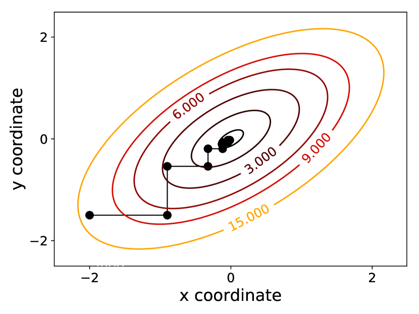
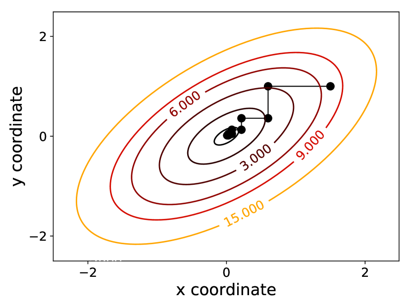
Block coordinate descent (BCD) methods are a universal approach to algorithmic optimization (wright2015coordinate). These iterative methods fix a block of components and optimize with respect to the remaining components. Figure 1 illustrates the process for a simple 2-dimensional function $f(x,y)$, where we iteratively update $x$ while $y$ is fixed

$$x=x+\nu\dfrac{\partial f}{\partial x}(x,y),$$

and $y$ while $x$ is fixed

$$y=y+\nu\dfrac{\partial f}{\partial y}(x,y),$$

until convergence is reached. The parameter $\nu$ controls the step size and can be chosen in various ways (wright2015coordinate). Following this philosophy, the HALS algorithm unbundles the original problem into a sequence of simpler optimization problems. This allows the efficient computation of the NMF (cichocki2009fast).

(a) Starting point $x=-2$ and $y=-1.5$.

(b) Starting point $x=1.5$ and $y=1.0$.

Figure 1: Coordinate descent finds the minimum of a function by successively updating only along one coordinate direction ($x$ or $y$) at a time, while fixing the other direction. In other words, a single variable optimization problem is solved in each iteration.

Suppose that we update $\mathbf{W}$ and $\mathbf{H}$ by fixing most terms except for the block comprised of the $j$th column $\mathbf{W}_{(:,j)}$ and $j$th row $\mathbf{H}_{(j,:)}$. Thus, each subproblem is essentially reduced to a smaller minimization. HALS approximately minimizes the cost function in Equation (2) with respect to the remaining $k-1$ components

$$\underset{}{\text{minimize}} J_{j}({\bf W}_{(:,j)},{\bf H}_{(j,:)})=\|\mathbf{R}^{(j)}-\mathbf{W}_{(:,j)}\mathbf{H}_{(j,:)}\|_{F}^{2},$$ (9)

where $\mathbf{R}^{(j)}$ is the $j$th residual

$$\mathbf{R}^{(j)}:=X-\sum_{i\neq j}^{k}{\bf W}_{(:,i)}{\bf H}_{(i,:)}.$$ (10)

This can be viewed as a decomposition of the residual (pmlr-v39-kimura14). Then, it is simple to derive the gradients to find the stationary points for both components. First, we expend the cost function in Eq. (9) as

$$J_{j} =\operatorname{Tr}\left[\mathbf{R}^{(j)\top}\mathbf{R}^{(j)}-2\mathbf{R}^{(j)\top}\mathbf{W}_{(:,j)}\mathbf{H}_{(j,:)}+\mathbf{H}_{(j,:)}^{\top}\mathbf{W}_{(:,j)}^{\top}\mathbf{W}_{(:,j)}\mathbf{H}_{(j,:)}\right]$$

$$=\|\mathbf{R}^{(j)}\|_{F}^{2}-2\operatorname{Tr}\left[\mathbf{R}^{(j)\top}\mathbf{W}_{(:,j)}\mathbf{H}_{(j,:)}\right]+\operatorname{Tr}\left[\mathbf{H}_{(j,:)}^{\top}\mathbf{W}_{(:,j)}^{\top}\mathbf{W}_{(:,j)}\mathbf{H}_{(j,:)}\right]$$

Then, we take the gradient of $\mathbf{W}(:,j)$ with respect to $J_{j}$

$$0=\frac{\partial J_{j}}{\partial{\bf W}_{(:,j)}}={\bf W}_{(:,j)}{\bf H}_{(j,:)}{\bf H}^{\top}_{(j,:)}-\mathbf{R}^{(j)}{\bf H}^{\top}_{(j,:)},$$

and the gradient of $\mathbf{H}(j,:)$ with respect to $J_{j}$

$$0=\frac{\partial J_{j}}{\partial{\bf H}_{(j,:)}}={\bf H}^{\top}_{(j,:)}{\bf W}^{\top}_{(:,j)}{\bf W}_{(:,j)}-\mathbf{R}^{(j)\top}{\bf W}_{(:,j)}.$$

The update rules for the $j$th component of ${\bf W}$ and ${\bf H}$ are

$${\bf W}_{(:,j)}^{+}\leftarrow\left[\frac{[\mathbf{R}^{(j)}{\bf H}^{\top}_{(j,:)}}{{\bf H}_{(j,:)}{\bf H}^{\top}_{(j,:)}}\right]_{+},$$ (11)

$${\bf H}_{(j,:)}^{+}\leftarrow\left[\frac{\mathbf{R}^{(j)\top}{\bf W}_{(:,j)}}{{\bf W}^{\top}_{(:,j)}{\bf W}_{(:,j)}}\right]_{+},$$ (12)

where the maximum operator, defined as $[x]_{+}:=\text{max}(0,x)$, ensures that the components remain nonzero. Note, that we can express Eq. (10) also as

$$\mathbf{R}^{(j)} :=\mathbf{X}-\sum_{i\neq j}^{k}\mathbf{W}_{(:,i)}\mathbf{H}_{(i,:)}=\mathbf{X}-\mathbf{W}\mathbf{H}+\mathbf{W}_{(:,j)}\mathbf{H}_{(j,:)}.$$ (13)

Then, Eq. 13 can be substituted into the above update rules in order to avoid the explicit computation of the residual $\mathbf{R}^{(j)}$. Hence, we obtain the following simplified update rules:

$$\mathbf{W}_{(:,j)}^{+}\leftarrow\left[\mathbf{W}_{(:,j)}+\frac{\left[\mathbf{X}\mathbf{H}^{\top}\right]_{(:,j)}-\mathbf{{W}}\left[\mathbf{H}\mathbf{H}^{\top}\right]_{(:,j)}}{\left[\mathbf{H}\mathbf{H}^{\top}\right]_{(j,j)}}\right]_{+},$$ (14)

$$\mathbf{H}_{(j,:)}^{+}\leftarrow\left[\mathbf{H}_{(j,:)}+\frac{\left[\mathbf{X}^{\top}\mathbf{W}\right]_{(:,j)}-\mathbf{H}^{\top}\left[\mathbf{W}^{\top}\mathbf{W}\right]_{(:,j)}}{[\mathbf{W}^{\top}\mathbf{W}]_{(j,j)}}\right]_{+}.$$ (15)

3.2 Randomized Hierarchal Alternating Least Squares

Employing randomness, we reformulate the optimization problem in Equation (2) as a low-dimensional optimization problem. Specifically, the high-dimensional $m\times n$ input matrix $\mathbf{X}$ is replaced by the $k\times n$ surrogate matrix $\mathbf{B}$, which is formed as described in Section 2.3. Thus we yield the following optimization problem:

$$\underset{}{\text{minimize}} \tilde{f}(\mathbf{\tilde{W}},\mathbf{H})=\|\mathbf{B-\tilde{W}H}\|_{F}^{2}$$ (16)

subject to $${\bf Q\tilde{W}\geq 0}\text{ and }{\bf H\geq 0}.$$

The nonnegativity constraints need to apply to the high-dimensional factor matrix ${\bf W}$, but not necessarily to ${\bf\tilde{W}}$. The matrix ${\bf\tilde{W}}$ can be rotated back to high-dimensional space using the following approximate relationship ${\bf W\approx Q\tilde{W}}$. Equation (16) can only be solved approximately, since ${\bf QQ^{\top}\neq I}$. Further, there is no reason that ${\bf\tilde{W}}$ has nonnegative entries, yet the low-dimensional projection will decrease the objective function in Equation (16). Now, we formulate the randomized HALS algorithm as

$$\underset{}{\text{minimize}} \tilde{J}_{j}({\bf\tilde{W}}_{(:,j)},{\bf H}_{(j,:)})=\|\mathbf{\tilde{R}}^{(j)}-\mathbf{\tilde{W}}_{(:,j)}\mathbf{H}_{(j,:)}\|_{F}^{2},$$ (17)

where $\mathbf{\tilde{R}}^{(j)}$ is the $j$th compressed residual

$$\mathbf{\tilde{R}}^{(j)}:=\mathbf{B}-\sum_{i\neq j}^{k}{\bf\tilde{W}}_{(:,i)}{\bf H}_{(i,:)}.$$ (18)

Then, the update rule for the $j$th component of $\mathbf{H}$ is as follows

$$\mathbf{H}_{(j,:)}^{+}\leftarrow\left[\mathbf{H}_{(j,:)}+\frac{\left[\mathbf{B}^{\top}\mathbf{\tilde{W}}\right]_{(:,j)}-\mathbf{H}^{\top}\left[\mathbf{\tilde{W}}^{\top}\mathbf{\tilde{W}}\right]_{(:,j)}}{[\mathbf{\tilde{W}}^{\top}\mathbf{\tilde{W}}]_{(j,j)}}\right]_{+},$$ (19)

Note, that we use $[\mathbf{{W}}^{\top}\mathbf{{W}}]_{(j,j)}$ for scaling in practice in order to ensure the correct scaling in high-dimensional space. Next, the update rule for the $j$th component of $\mathbf{\tilde{W}}$ is

$$\mathbf{\tilde{W}}_{(:,j)}\leftarrow\mathbf{\tilde{W}}_{(:,j)}+\frac{\left[\mathbf{B}\mathbf{H}^{\top}\right]_{(:,j)}-\mathbf{\tilde{W}}\left[\mathbf{H}\mathbf{H}^{\top}\right]_{(:,j)}}{\left[\mathbf{H}\mathbf{H}^{\top}\right]_{(j,j)}}.$$ (20)

Then, we employ the following scheme to update the $j$th component in high-dimensional space, followed by projecting the updated factor matrix $\mathbf{W}^{+}$ back to low-dimensional space

$${\bf{W}}_{(:,j)}^{+}\leftarrow[{\bf Q\tilde{W}}_{(:,j)}]_{+}.$$ (21)

$${\bf\tilde{W}}_{(:,j)}^{+}\leftarrow{\bf Q}^{\top}{\bf{W}}_{(:,j)}^{+}.$$ (22)

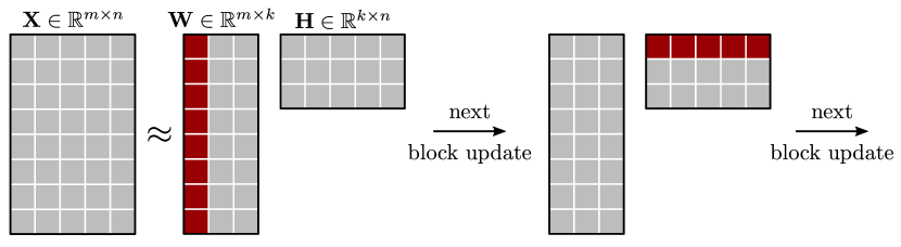
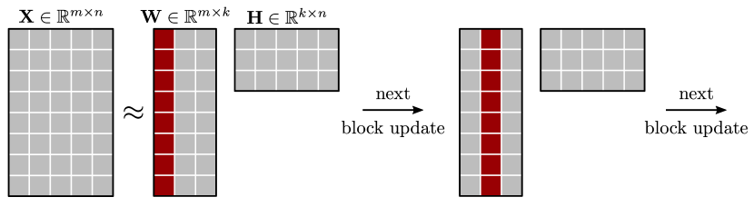
This HALS framework allows the choice of different update orders (kim2014algorithms). For instance, we can proceed by using one of the following two cyclic update orders:

$${\bf{W}}_{(:,1)}^{+}\rightarrow{\bf{H}}_{(1,:)}^{+}\rightarrow\dots\rightarrow{\bf{W}}_{(:,k)}^{+}\rightarrow{\bf{H}}_{(k,:)}^{+},$$ (23)

or

$${\bf{W}}_{(:,1)}^{+}\rightarrow{\bf{W}}_{(:,2)}^{+}\rightarrow\dots\rightarrow{\bf{W}}_{(:,k)}^{+}\rightarrow{\bf{H}}_{(1,:)}^{+}\rightarrow{\bf{H}}_{(2,:)}^{+}\dots\rightarrow{\bf{H}}_{(k,:)}^{+},$$ (24)

which are illustrated in Figure 2. We favor the latter scheme in the following. Alternatively, a shuffled update order can be used, wherein the components are updated in a random order in each iteration. wright2015coordinate noted that this scheme performs better in some applications. Yet another exciting strategy is randomized block coordinate decent (nesterov2012efficiency).

(a) Update order: ${\bf{W}}_{(:,1)}^{+}\rightarrow{\bf{H}}_{(1,:)}^{+}\rightarrow\dots\rightarrow{\bf{W}}_{(:,k)}^{+}\rightarrow{\bf{H}}_{(k,:)}^{+}$.

(b) Update order:${\bf{W}}_{(:,1)}^{+}\rightarrow{\bf{W}}_{(:,2)}^{+}\rightarrow\dots\rightarrow{\bf{W}}_{(:,k)}^{+}\rightarrow{\bf{H}}_{(1,:)}^{+}\rightarrow{\bf{H}}_{(2,:)}^{+}\dots\rightarrow{\bf{H}}_{(k,:)}^{+}$.

Figure 2: Cyclic update orders.

The computational steps are summarized in Algorithm LABEL:alg:rHALS.

3.3 Stopping Criterion

Predefining a maximum number of iterations is not satisfactory in practice. Instead, we aim to stop the algorithm when a suitable measure has reached some convergence tolerance. For a discussion on stopping criteria, for instance, see gillis2012accelerated. One option is to terminate the algorithm if the value of objective function is smaller than some stopping condition $\epsilon$

$$||\mathbf{X}-\mathbf{W}\mathbf{H}||_{F}^{2}<\epsilon.$$ (25)

This criteria is expensive to compute and often not a good measure for convergence. An interesting alternative stopping condition is the projected gradient (lin2007projected; hsieh2011fast). The projected gradient $\nabla^{P}f(\mathbf{W,H})$ measures how close the current solution is to a stationary point. We compute the projected gradient with respect to $\mathbf{W}$ as

$$\nabla^{P}_{\mathbf{W}_{ij}}:=\begin{cases}\dfrac{\partial f(\mathbf{W,H})}{\partial\mathbf{W}_{ij}},&\text{if}\ \mathbf{W}_{ij}>0\\ min(0,\dfrac{\partial f(\mathbf{W,H})}{\partial\mathbf{W}_{ij}}),&\text{if}\ \mathbf{W}_{ij}=0\\ \end{cases},$$ (26)

and in a similar way with respect to $\mathbf{H}$. Accordingly, the stopping condition can be formulated:

$$||\nabla^{P}f(\mathbf{W,H})||_{F}^{2}<\epsilon||\nabla^{P}f(\mathbf{W^{0},H^{0}})||_{F}^{2},$$ (27)

where $\mathbf{W^{0}}$ and $\mathbf{H^{0}}$ indicate the initial points. Note, that it follows from the Karush–Kuhn–Tucker (KKT) condition that a stationary point is reached if and only if the projected gradient is $\nabla^{P}f(\mathbf{W^{*},H^{*}})=0$ for some optimal points $\mathbf{W^{*}}$ and $\mathbf{H^{*}}$.

Require: A nonnegative matrix $\mathbf{X}$ of dimension $m\times n$, and target rank $k$.

Optional: Parameters $p$ and $q$ for oversampling, and power iterations.

(1) $l=k+p$ Slight oversampling

(2) $\mathbf{\Omega}=\texttt{rand}(n,l)$ $\textrm{Generate sampling matrix }\mathbf{\Omega}\in\mathbb{R}^{n\times l}$

(3) $\mathbf{Y}=\mathbf{X}\mathbf{\Omega}$ $\textrm{Form basis }\mathbf{Y}\in\mathbb{R}^{m\times l}$

(4) for $j=1,\dots,q$ Optional: subspace iterations

(5) $\left[\mathbf{Q},\sim\right]=\texttt{qr}(\mathbf{Y})$

(6) $\left[\mathbf{Q},\sim\right]=\texttt{qr}(\mathbf{\mathbf{X}^{\top}\mathbf{Q}})$

(7) $\mathbf{Y}=\mathbf{X}\mathbf{Q}$

(8) $\left[\mathbf{Q},\sim\right]=\texttt{qr}(\mathbf{Y})$ Form orthonormal basis $\mathbf{Q}\in\mathbb{R}^{m\times l}$

(9) $\mathbf{B}=\mathbf{Q}^{\top}\mathbf{X}$ $\textrm{Form smaller matrix }\mathbf{B}\in\mathbb{R}^{l\times n}$

(10) Initialize nonnegative factors $\mathbf{W}\in\mathbb{R}^{m\times k}$, $\mathbf{\tilde{W}}\in\mathbb{R}^{l\times k}$ and $\mathbf{H}\in\mathbb{R}^{k\times n}$

(11) repeat

(12) $\mathbf{R}=\mathbf{B}^{\top}\mathbf{\tilde{W}}$ $\mathbf{R}\in\mathbb{R}^{n\times k}$

(13) $\mathbf{S}=\mathbf{{W}}^{\top}\mathbf{{W}}$ $\mathbf{S}\in\mathbb{R}^{k\times k}$

(14) for $j=1,\dots,k$ Update $\mathbf{H}$ row by row

(15)