Anisotropic emission of neutrino and gravitational-wave signals from rapidly rotating core-collapse supernovae

Abstract

We present analysis on neutrino and GW signals based on three-dimensional (3D) core-collapse supernova simulations of a rapidly rotating 27 $M_{\odot}$ star. We find a new neutrino signature that is produced by a lighthouse effect where the spinning of strong neutrino emission regions around the rotational axis leads to quasi-periodic modulation in the neutrino signal. Depending on the observer’s viewing angle, the time modulation will be clearly detectable in IceCube and the future Hyper-Kamiokande. The GW emission is also anisotropic where the GW signal is emitted, as previously identified, most strongly toward the equator at rotating core-collapse and bounce, and the non-axisymmetric instabilities in the postbounce phase lead to stronger GW emission toward the spin axis. We show that these GW signals can be a target of LIGO-class detectors for a Galactic event. The origin of the postbounce GW emission naturally explains why the peak GW frequency is about twice of the neutrino modulation frequency. We point out that the simultaneous detection of the rotation-induced neutrino and GW signatures could provide a smoking-gun signature of a rapidly rotating proto-neutron star at the birth.

1 Introduction

Detection of neutrinos and gravitational waves (GWs) from core-collapse supernovae (CCSNe) has been long expected to provide crucial information for understanding the explosion mechanism (e.g., Mirizzi et al. (2016); Kotake (2013) for a review). Currently multiple neutrino detectors are in operation, where the best suited ones for detecting CCSN neutrinos are Super-Kamiokande and IceCube (e.g., Scholberg (2012)). Ever since SN1987A, significant progress has been also made in GW detectors. The high sensitivity led to the Nobel-prize-awarded detection by the LIGO collaboration (Abbott et al., 2016) from the black hole merger event. Virgo also reported the first joint GW detection (The LIGO Scientific Collaboration and the Virgo Collaboration et al., 2017). KAGRA will start the operation in the coming years (Aso et al., 2013). Targeted by these multi-messenger observations, the importance of neutrino and GW predictions from CCSNe is ever increasing.

From the CCSN theory and simulations, it is almost certain that multi-dimensional (multi-D) hydrodynamics instabilities including neutrino-driven convection and the Standing-Accretion-Shock-Instability (SASI) play a crucial role in facilitating the neutrino mechanism of CCSNe (Bethe (1990), see Burrows (2013); Janka et al. (2016) for review). In fact, a number of self-consistent models in two or three spatial dimensions (2D, 3D) now report revival of the stalled bounce shock into explosion by the multi-D neutrino mechanism (see, e.g., Müller et al. (2017); Bollig et al. (2017); Roberts et al. (2016); Melson et al. (2015); Lentz et al. (2015); Nakamura et al. (2015) for collective references therein).

In order to get a more robust and sufficiently energetic explosion to meet with observations, some physical ingredients may be still missing (e.g., Janka et al. (2016)). Possible candidates to enhance the chance of explodability include general relativity (e.g., Müller et al. (2012); Kuroda et al. (2012); Roberts et al. (2016)), inhomogenities in the progenitor’s burning shells (e.g., Couch & Ott (2015); Müller & Janka (2015)), rotation (Marek & Janka, 2009; Suwa et al., 2010; Takiwaki et al., 2016; Summa et al., 2017) and magnetic fields (e.g., Mösta et al. (2015); Guilet & Müller (2015); Rembiasz et al. (2016); Obergaulinger & Aloy (2017)).

In our previous work, we reported a new type of rotation-assisted, neutrino-driven explosion of a $27M_{\odot}$ star (Takiwaki et al., 2016), where the growth of non-axisymmetric instabilities due to the so-called low-T/|W| instability is the key to foster the onset of the explosion. More recently, Summa et al. (2017) found yet another type of rotation-assisted, neutrino-driven explosion of a 15 $M_{\odot}$ star where the powerful spiral SASI motions play a crucial role in driving the explosion. Note that the GW signals from rapidly rotating core-collapse and bounce have been extensively studied so far (e.g., Dimmelmeier et al. (2008); Ott (2009); Scheidegger et al. (2010); Kuroda et al. (2014)). The correlation of the neutrino and GW signals from rapidly rotating models have been studied in 3D models (Ott et al., 2012) with octant symmetry focusing on the bounce signature (limited to $\sim 30$ ms postbounce) and in Yokozawa et al. (2015) based on their 2D models. However, the postbounce GW and neutrino signals have not yet been studied in the context of self-consistent, 3D neutrino-driven models aided by rotation.

In this Letter, we present analysis of neutrino and GW signals from the rotation-aided, neutrino-driven explosion of a $27M_{\odot}$ star in Takiwaki et al. (2016). We find a new neutrino signature that is produced by a neutrino lighthouse effect. We discuss the detectability in IceCube and the future Hyper-Kamiokande. By combining with the postbounce GW signatures, we find that the peak GW frequency is physically linked to the peak neutrino modulation frequency. We point out that these signatures, if simultaneously detected, could provide evidence of rapid rotation of the forming PNS.

2 Numerical Methods

From our 3D models computed in Takiwaki et al. (2016), we take the rotation-assisted explosion model of $27.0$ $M_{\odot}$ star ("s27.0-R2.0-3D") for the analysis in this work. For the model, the constant angular frequency of $\Omega_{0}=2$ rad/s is initially imposed to the iron core of a non-rotating progenitor of Woosley et al. (2002) with a cut-off ($\propto r^{-2}$) outside. We employ the isotropic diffusion source approximation (IDSA) scheme (Liebendörfer et al., 2009) for spectral neutrino transport of electron-($\nu_{e}$) and anti-electron-($\bar{\nu}_{e}$) neutrinos and a leakage scheme for heavy-lepton neutrinos ($\nu_{x}$) (see Takiwaki et al. (2016) for more details). Note that our 3D run failed to explode in the absence of rotation (Takiwaki et al., 2016), which is in line with Hanke et al. (2013) who performed 3D full-scale simulations using the same progenitor but with more elaborate neutrino transport scheme.

We consider two water Čerenkov neutrino detectors, IceCube (Abbasi et al., 2011; Salathe et al., 2012) and the future Hyper-Kamiokande (Abe et al., 2011; Hyper-Kamiokande proto-collaboration, 2016). In the detectors, the main detection channel is of anti-electron neutrino ($\bar{\nu}_{e}$) with inverse-beta decay (IBD). The observed event rate at Hyper-Kamiokande is calculated as follows,

$$R_{\rm HK}=N_{\rm p}\int_{E_{\rm th}}{\rm d}E_{e}\frac{{\rm d}F_{\bar{\nu}_{e}}}{{\rm d}E_{\nu}}\sigma\left(E_{\nu}\right)\frac{{\rm d}E_{\nu}}{{\rm d}E_{e}},$$ (1)

where $N_{\rm p}=2.95\times 10^{34}$ is the number of protons for two tanks of Hyper-Kamiokande whose fiducial volume is designed as 440 kton, $E_{\rm th}=7~{}{\rm MeV}$ is the threshold energy, $\sigma$ is the cross section of the IBD (Fukugita & Yanagida, 2003). The neutrino number flux of $\bar{\nu}_{e}$ ($F_{\bar{\nu}_{e}}$) at a source distance of $D$ is estimated as $F_{\bar{\nu}_{e}}=\frac{\mathcal{L}_{\Omega}}{4\pi D^{2}}$, where $\mathcal{L}_{\Omega}$ denotes an viewing-angle dependent neutrino (number) luminosity (see Appendix A of Tamborra et al. (2014)). In this work, $D$ is set as $10$ kpc unless otherwise stated. Following Keil et al. (2003), the neutrino spectrum is assumed to take a Fermi-Dirac distribution with vanishing chemical potential (see their Eq. (5)).

While individual neutrino events cannot be reconstructed, a statistically significantly "glow" is predicted to be observed during the passage of the CCSN neutrino signals at IceCube (e.g., (Mirizzi et al., 2016)). We estimate the event rate at IceCube following Equation (2) in Lund et al. (2010).

Extraction of GWs from our simulations is done by using the conventional quadrupole stress formula (Misner et al., 1973; Müller & Janka, 1997). For numerical convenience, we employ the first-moment-of-momentum-divergence (FMD) formalism proposed by Finn & Evans (1990) (see also Murphy et al. (2009); Müller et al. (2013), and Takiwaki & Kotake (2011) for justification.)

3 Results

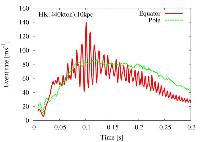
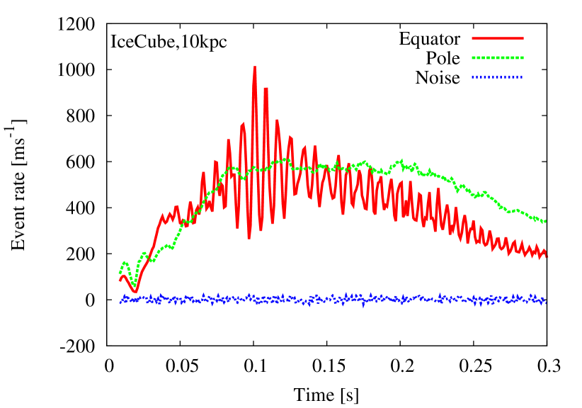
Figure 1: Hyper-Kamiokande (HK, upper) and IceCube (lower) detection rates of $\bar{\nu}_{e}$ at 10 kpc for our rapidly rotating $27M_{\odot}$ model as a function of time after bounce. The red and green line corresponds to the event rates (per 1 ms bin) for an observer along the equator and the pole, respectively. In both of the detectors, a quasi-periodic modulation (red lines) is clearly seen for the observer along the equator. For IceCube, the background fluctuations are shown by blue line.

Figure 1 shows the expected neutrino signals for our rapidly rotating $27M_{\odot}$ star at Hyper-Kamiokande (top panel) and IceCube (lower panel), respectively. In both of the detectors, a quasi-periodic modulation (red lines) is clearly seen for an observer along the equator, which cannot be seen for an observer along the rotational axis (denoted as "Pole" in the panel, green lines). The modulation amplitude at Hyper-Kamiokande (top panel, red line) is significantly higher than the root-N Poisson errors, $\sqrt{N}\sim\sqrt{R_{\rm HK}\times 1{\rm ms}}\sim 9$. For IceCube, much bigger modulation amplitudes are obtained due to its large volume. This is well above the IceCube background noise (blue line) of $\sim\sqrt{R_{\rm bkgd}\times 1{\rm ms}}\sim 38$ for the 1ms bin (Tamborra et al., 2013). For a source at 10 kpc, IceCube plays a crucial role for detecting the signal modulation. But, for the more distant source, Hyper-Kamiokande can be superior because it is essentially background free (see Scholberg (2012) for detail).

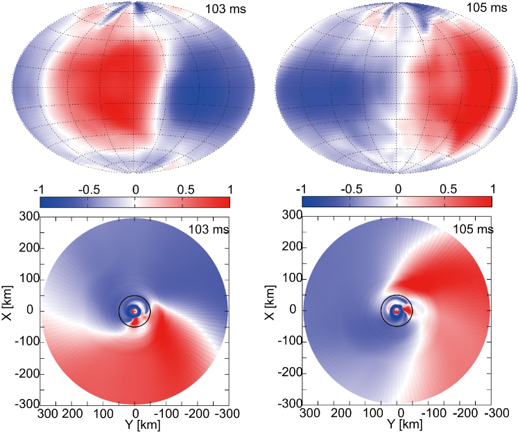
Figure 2: Rotation of the anisotropic $\bar{\nu}_{e}$ flux around the spin axis. Top panels show the deviation of the flux from the angle-averaged one ($\delta F_{\bar{\nu}_{e}}$, Eq.(2)) at two snapshots of 103 ms (left panels) and 105 ms (right panels) after bounce, respectively. In the skymaps using the Hammer projection, the latitudes and longitudes are indicated by the dotted lines. Similar to the top panels, but the bottom panels display $\delta F_{\bar{\nu}_{e}}$ on the equatorial plane ($z=0$). The high neutrino emission region (colored by red) rotates in a counterclockwise direction from the bottom left to the bottom right panel (compare also the top left with the top right panel).

The clear signal modulation of Figure 1 originates from a strong neutrino emitter rotating around the spin axis. This is essentially in analogue to a lighthouse effect as we will explain in detail below. Figure 2 visualizes this, where the top two panels show how the excess in the anisotropic $\bar{\nu}_{e}$ flux (red regions) moves in the skymaps. Here we estimate the degree of local anisotropic $\bar{\nu}_{e}$ flux as

$$\delta F_{\bar{\nu}_{e}}=\frac{F_{\bar{\nu}_{e}}-\langle F_{\bar{\nu}_{e}}\rangle}{\sqrt{\langle\left(F_{\bar{\nu}_{e}}-\langle F_{\bar{\nu}_{e}}\rangle\right)^{2}}\rangle},$$ (2)

where $F_{\bar{\nu}_{e}}$ is the flux measured at a radius of 500 km and $\langle F_{\bar{\nu}_{e}}\rangle$ is the angle-averaged one. In the skymaps, the direction where the flux is strong (weak) is colored by red (blue). The left and right panels correspond to the snapshot at 103 ms and 105 ms after bounce, respectively. At 103 ms (top left panel), the high neutrino emission region (colored by red) looks mostly concentrated in the western side in the skymap. More precisely, the highest neutrino emission comes from the direction near at the center of the skymap $(\theta,\phi)\approx(\frac{\pi}{2},\pi)$. And the high emission region is shown to move to the right (or eastern) direction in the top right panel at 105 ms after bounce, where the highest emission region is shifting to the direction at $(\theta,\phi)\approx(\frac{\pi}{2},\frac{3\pi}{2})$ due to rotation of the hot spot. The neutrino event rates become biggest when the hot spot directly points to the observer.

Looking into more details, we show that the time modulation of Figure 1 originally comes from rotation of the anisotropic $\bar{\nu}_{e}$ flux at the neutrino sphere. The bottom panels of Figure 2 show the degree of the anisotropic $\bar{\nu}_{e}$ flux ($\delta F_{\bar{\nu}_{e}}$) in the equatorial plane (i.e., seen from the direction parallel to the spin axis). In the panels, the black circle drawn at a radius of 50 km roughly corresponds to the (average) $\bar{\nu}_{e}$ sphere. In the bottom left panel, the excess of $\delta F_{\bar{\nu}_{e}}$ (colored by red) is strongest at $(X,Y)=(-300,0)$, corresponding to $(\theta,\phi)\approx(\frac{\pi}{2},\pi)$ in the top left panel. At 2 ms later, the bottom right panel shows that the central region rotates counterclockwisely, making the hot spot rotate simultaneously to the right direction at $(X,Y)=(0,-300)$. Again this corresponds to the red region in the top right panel at $(\theta,\phi)\approx(\frac{\pi}{2},\frac{3\pi}{2})$.

The rotation of the anisotropic neutrino emission seen in Figure 2 is associated with the one-armed spiral flows. As already discussed in Takiwaki et al. (2016), the growth of the spiral flows is triggered by the low-$T/|W|$ instability. Like a screw, the non-axisymmetric flows initially develop from the PNS surface at a radius of 20 km (e.g., middle panel of Figure 3 of Takiwaki et al. (2016)), then penetrate into the $\bar{\nu}_{e}$ sphere (e.g., black circle in the bottom panels of Figure 2), leading to the anisotropic neutrino emission. Rotation of the anisotropic $\bar{\nu}_{e}$ flux at the neutrino sphere is the origin of the neutrino lighthouse effect, leading to the observable modulation in the neutrino signal as shown in Figure 1.

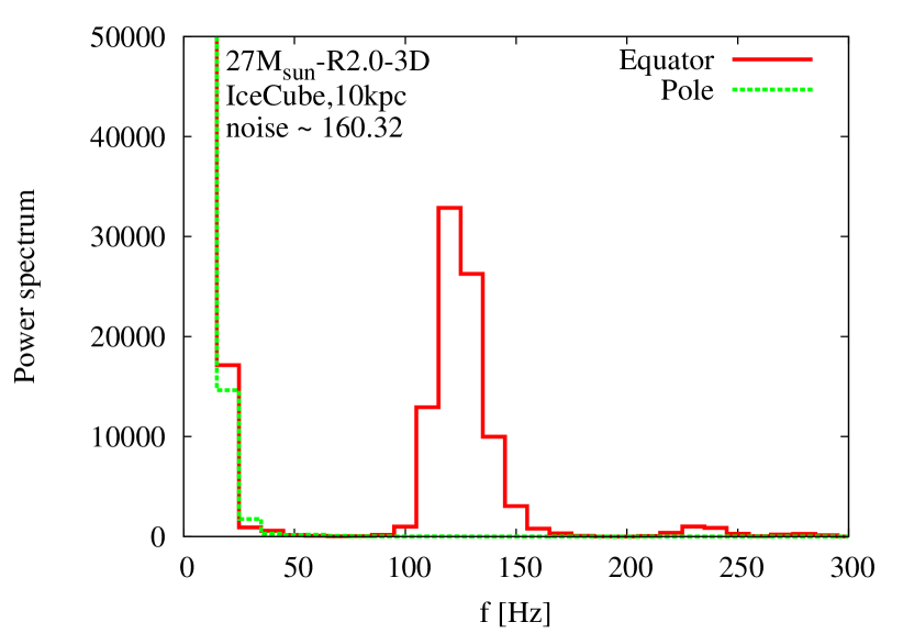
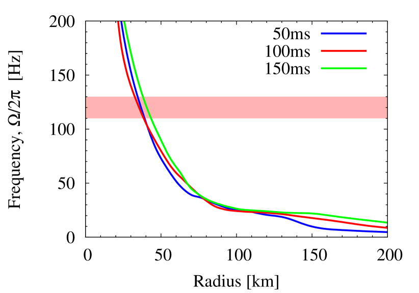
Figure 3: Similar to Figure 1 (lower) but for the power spectrum of the IceCube event rate on the interval of 100 ms (from 50 to 150 ms after bounce). A pronounced peak can be seen at $\sim$ 120 Hz (red line) for an observer in the equatorial direction (labeled as "Equator" ). Bottom panel shows radial profiles of the rotational frequency of the matter at three postbounce times of 50 ms (blue line), 100 ms (red line) and 150 ms (green line), respectively. The rotational frequency is estimated from the (azimuthally-averaged) angular velocity as $\Omega/2\pi$. The horizontal pink band approximately corresponds to the peak frequency in the spectrum with the HWHM contribution ($120\pm 10$ Hz).

The top panel of Figure 3 shows power spectrum of the IceCube event rate on the interval of 100 ms after bounce. Seen from the equator (red line), one can clearly see a peak around 120 Hz, which cannot be seen from the pole (green line). Following Lund et al. (2010) (e.g., their Appendix A and Eq. (12)), the noise level of the IceCube is estimated as 160.32 (for the 100 ms time interval). This is significantly lower than the peak amplitude (red line) at a 10 kpc distance scale.

The bottom panel of Figure 3 shows that the matter rotational frequency (at three different postbounce times) closely matches with the neutrino modulation frequency (horizontal pink band, $120\pm 10$ Hz) at a radius of $40\sim 50$ km, which corresponds to the $\bar{\nu}_{e}$ sphere radius. This also supports the validity of the concept of the neutrino lighthouse effect firstly proposed in this work.

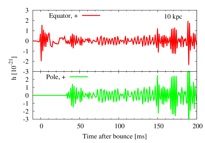
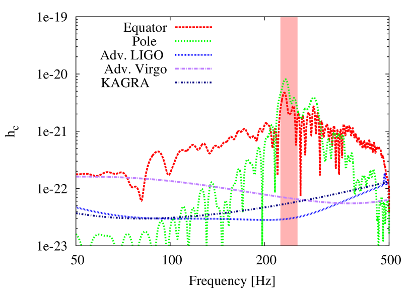
Figure 4: Top panel shows the GW amplitude of plus mode for observers along the equator (red line) and the pole (green line) for a source at 10 kpc. The bottom panel shows the characteristic GW spectra relative to the sensitivity curves of advanced LIGO (Harry & LIGO Scientific Collaboration, 2010), advanced Virgo (Hild et al., 2009) and KAGRA (Aso et al., 2013). Note in the bottom plot, we focus on only the frequency range ($\lesssim$ 500 Hz) with the maximum sensitivity.

Finally we shortly discuss the GW signatures from our 3D model. The top panel of Figure 4 shows the GW amplitude (plus mode) for observers along the equator (red line) and along the pole (green line), respectively. Seen from the equator (red line), the waveform after bounce is characterized by a big spike followed by the ring-down phase (up to $\sim$ 30 ms after bounce). This is the most generic waveform from rapidly rotating core-collapse and bounce (Dimmelmeier et al., 2008), also known as the type I waveform. Seen from the spin axis (green line), the GW amplitude deviates from zero only after $\sim 40$ ms postbounce when the non-axisymmetric instabilities start to develop most strongly in the equatorial region. The wave amplitude is thus bigger for the polar observer compared to the equatorial observer. Note that the polar-to-equator contrast in the GW amplitude is stronger for the cross mode (not shown in the plot) than the plus mode. These features are consistent with those obtained in previous 3D models (Scheidegger et al., 2010; Ott, 2009) but with more approximate neutrino treatments.

The bottom panel of Figure 4 shows the characteristic GW spectra ($h_{c}$) relative to the sensitivity curves of advanced LIGO and KAGRA for a source at 10 kpc. Seen either from the equator (red line) or the pole (green line), the peak GW frequency is around 240Hz (e.g., the pink vertical band). Note that this is about twice as large as that of the modulation frequency of the neutrino signal ($\sim$ 120 Hz). This is simply because a deformed object rotating around the spin axis in the frequency of $f$ emits the quadrupole GW radiation with the frequency of $2f$. Our results show that the non-axisymmetric flow induced by the low-T/|W| instability is the key to explain the correlation between the time modulation in the neutrino and GW signal in the context of rapidly rotating CCSNe. One can also see that the characteristic GW amplitude for the polar observer (green line) in absence of the bounce GW signal is more narrow-banded compared to that for the equatorial observer (red line). As one would expect, the maximum $h_{c}$ at the peak GW frequency ($\sim$ 240 Hz) is bigger for the polar observer than that for the equatorial observer. It should be noted that the peak frequency is close to the maximum sensitivities of advanced LIGO, advanced Virgo, and KAGRA. These neutrino and GW signatures, if simultaneously detected, could provide new evidence of rapid rotation of the forming PNS.

4 Discussion

For enhancing our predictive power of the neutrino and GW signals, we have to update our numerical schemes in many respects. These include general relativistic effects with an improved multipole approximation of gravity (Couch et al., 2013), multi-angle treatment in neutrino transport (e.g., Sumiyoshi et al. (2015)) beyond our ray-by-ray approximation using more detailed neutrino opacities (e.g., Burrows et al. (2006)). Given the rapidly rotating PNS, magnetic fields should be also taken into account (e.g., Mösta et al. (2015)), where the field amplification due to the magneto-rotational instability (e.g., Obergaulinger et al. (2009); Masada et al. (2015)) could potentially affect the explosion dynamics. To test this, a high-resolution 3D MHD model is needed, which is another major undertaking. Finally it is noted that in the 3D model of the 11.2 $M_{\sun}$ progenitor (Takiwaki et al., 2016) no clear signatures as in Figures 1 and 4 are obtained. This is because the 11.2 $M_{\sun}$ model explodes even without rotation where the low T/|W| instability does not develop during the simulation time. In order to clarify how general the correlated signatures found in this work would be, systematic 3D simulations changing the progenitor masses and initial rotation rates are needed, which we leave as a future work.

5 Acknowledgements

The computations in this research were performed on the K computer of the RIKEN AICS through the HPCI System Research project (Project ID:hp120304) together with XC30 of CfCA in NAOJ. This study was supported by JSPS KAKENHI Grant Number (JP15H01039, JP15H00789, JP15KK0173, JP17H06364, JP17K14306, and JP17H01130) and JICFuS as a priority issue to be tackled by using Post ’K’ computer.

References

- Abbasi et al. (2011) Abbasi R., et al., 2011, A&A, 535, A109
- Abbott et al. (2016) Abbott B. P., et al., 2016, Physical Review Letters, 116, 061102
- Abe et al. (2011) Abe K., et al., 2011, preprint, (arXiv:1109.3262)
- Aso et al. (2013) Aso Y., Michimura Y., Somiya K., Ando M., Miyakawa O., Sekiguchi T., Tatsumi D., Yamamoto H., 2013, Phys. Rev. D, 88, 043007
- Bethe (1990) Bethe H. A., 1990, Reviews of Modern Physics, 62, 801
- Bollig et al. (2017) Bollig R., Janka H.-T., Lohs A., Martinez-Pinedo G., Horowitz C. J., Melson T., 2017, preprint, (arXiv:1706.04630)
- Burrows (2013) Burrows A., 2013, Reviews of Modern Physics, 85, 245
- Burrows et al. (2006) Burrows A., Reddy S., Thompson T. A., 2006, Nuclear Physics A, 777, 356
- Couch & Ott (2015) Couch S. M., Ott C. D., 2015, ApJ, 799, 5
- Couch et al. (2013) Couch S. M., Graziani C., Flocke N., 2013, ApJ, 778, 181
- Dimmelmeier et al. (2008) Dimmelmeier H., Ott C. D., Marek A., Janka H.-T., 2008, Phys. Rev. D, 78, 064056
- Finn & Evans (1990) Finn L. S., Evans C. R., 1990, ApJ, 351, 588
- Fukugita & Yanagida (2003) Fukugita M., Yanagida T., 2003, Physics of Neutrino, 2003 edn. Springer
- Guilet & Müller (2015) Guilet J., Müller E., 2015, MNRAS, 450, 2153
- Hanke et al. (2013) Hanke F., Müller B., Wongwathanarat A., Marek A., Janka H.-T., 2013, ApJ, 770, 66
- Harry & LIGO Scientific Collaboration (2010) Harry G. M., LIGO Scientific Collaboration 2010, Classical and Quantum Gravity, 27, 084006
- Hild et al. (2009) Hild S., Freise A., Mantovani M., Chelkowski S., Degallaix J., Schilling R., 2009, Classical and Quantum Gravity, 26, 025005
- Hyper-Kamiokande proto-collaboration (2016) Hyper-Kamiokande proto-collaboration 2016, KEK-PREPRINT-2016-21, ICRR-REPORT-701-2016-1
- Janka et al. (2016) Janka H.-T., Melson T., Summa A., 2016, Annual Review of Nuclear and Particle Science,
- Keil et al. (2003) Keil M. T., Raffelt G. G., Janka H.-T., 2003, ApJ, 590, 971
- Kotake (2013) Kotake K., 2013, Comptes Rendus Physique, 14, 318
- Kuroda et al. (2012) Kuroda T., Kotake K., Takiwaki T., 2012, ApJ, 755, 11
- Kuroda et al. (2014) Kuroda T., Takiwaki T., Kotake K., 2014, Phys. Rev. D, 89, 044011
- Lentz et al. (2015) Lentz E. J., et al., 2015, ApJ, 807, L31
- Liebendörfer et al. (2009) Liebendörfer M., Whitehouse S. C., Fischer T., 2009, ApJ, 698, 1174
- Lund et al. (2010) Lund T., Marek A., Lunardini C., Janka H.-T., Raffelt G., 2010, Phys. Rev. D, 82, 063007
- Marek & Janka (2009) Marek A., Janka H.-T., 2009, ApJ, 694, 664
- Masada et al. (2015) Masada Y., Takiwaki T., Kotake K., 2015, ApJ, 798, L22
- Melson et al. (2015) Melson T., Janka H.-T., Bollig R., Hanke F., Marek A., Müller B., 2015, ApJ, 808, L42
- Mirizzi et al. (2016) Mirizzi A., Tamborra I., Janka H.-T., Saviano N., Scholberg K., Bollig R., Hüdepohl L., Chakraborty S., 2016, Nuovo Cimento Rivista Serie, 39, 1
- Misner et al. (1973) Misner C. W., Thorne K. S., Wheeler J. A., 1973, Gravitation. Princeton University Press
- Mösta et al. (2015) Mösta P., Ott C. D., Radice D., Roberts L. F., Schnetter E., Haas R., 2015, Nature, 528, 376
- Müller & Janka (1997) Müller E., Janka H.-T., 1997, A&A, 317, 140
- Müller & Janka (2015) Müller B., Janka H.-T., 2015, MNRAS, 448, 2141
- Müller et al. (2012) Müller B., Janka H.-T., Heger A., 2012, ApJ, 761, 72
- Müller et al. (2013) Müller B., Janka H.-T., Marek A., 2013, ApJ, 766, 43
- Müller et al. (2017) Müller B., Melson T., Heger A., Janka H.-T., 2017, MNRAS, 472, 491
- Murphy et al. (2009) Murphy J. W., Ott C. D., Burrows A., 2009, ApJ, 707, 1173
- Nakamura et al. (2015) Nakamura K., Takiwaki T., Kuroda T., Kotake K., 2015, PASJ, 67, 107
- Obergaulinger & Aloy (2017) Obergaulinger M., Aloy M. Á., 2017, MNRAS, 469, L43
- Obergaulinger et al. (2009) Obergaulinger M., Cerdá-Durán P., Müller E., Aloy M. A., 2009, A&A, 498, 241
- Ott (2009) Ott C. D., 2009, Classical and Quantum Gravity, 26, 063001
- Ott et al. (2012) Ott C. D., et al., 2012, Phys. Rev. D, 86, 024026
- Rembiasz et al. (2016) Rembiasz T., Guilet J., Obergaulinger M., Cerdá-Durán P., Aloy M. A., Müller E., 2016, MNRAS, 460, 3316
- Roberts et al. (2016) Roberts L. F., Ott C. D., Haas R., O’Connor E. P., Diener P., Schnetter E., 2016, ApJ, 831, 98
- Salathe et al. (2012) Salathe M., Ribordy M., Demirörs L., 2012, Astroparticle Physics, 35, 485
- Scheidegger et al. (2010) Scheidegger S., Käppeli R., Whitehouse S. C., Fischer T., Liebendörfer M., 2010, A&A, 514, A51
- Scholberg (2012) Scholberg K., 2012, Annual Review of Nuclear and Particle Science, 62, 81
- Sumiyoshi et al. (2015) Sumiyoshi K., Takiwaki T., Matsufuru H., Yamada S., 2015, ApJS, 216, 5
- Summa et al. (2017) Summa A., Janka H.-T., Melson T., Marek A., 2017, preprint, (arXiv:1708.04154)
- Suwa et al. (2010) Suwa Y., Kotake K., Takiwaki T., Whitehouse S. C., Liebendörfer M., Sato K., 2010, PASJ, 62, L49
- Takiwaki & Kotake (2011) Takiwaki T., Kotake K., 2011, ApJ, 743, 30
- Takiwaki et al. (2016) Takiwaki T., Kotake K., Suwa Y., 2016, MNRAS, 461, L112
- Tamborra et al. (2013) Tamborra I., Hanke F., Müller B., Janka H.-T., Raffelt G., 2013, Physical Review Letters, 111, 121104
- Tamborra et al. (2014) Tamborra I., Raffelt G., Hanke F., Janka H.-T., Müller B., 2014, Phys. Rev. D, 90, 045032
- The LIGO Scientific Collaboration and the Virgo Collaboration et al. (2017) The LIGO Scientific Collaboration and the Virgo Collaboration et al., 2017, preprint, (arXiv:1709.09660)
- Woosley et al. (2002) Woosley S. E., Heger A., Weaver T. A., 2002, Reviews of Modern Physics, 74, 1015
- Yokozawa et al. (2015) Yokozawa T., Asano M., Kayano T., Suwa Y., Kanda N., Koshio Y., Vagins M. R., 2015, ApJ, 811, 86