Giant Molecular Cloud Collisions as Triggers of Star Formation. VI. Collision-Induced Turbulence

Abstract

We investigate collisions between giant molecular clouds (GMCs) as potential generators of their internal turbulence. Using magnetohydrodynamic (MHD) simulations of self-gravitating, magnetized, turbulent, GMCs, we compare kinematic and dynamic properties of dense gas structures formed when such clouds collide compared to those that form in non-colliding clouds as self-gravity overwhelms decaying turbulence. We explore the nature of turbulence in these structures via distribution functions of density, velocity dispersions, virial parameters, and momentum injection. We find that the dense clumps formed from GMC collisions have higher effective Mach number, greater overall velocity dispersions, sustain near-virial equilibrium states for longer times, and are the conduit for injection of turbulent momentum into high density gas at high rates.

1 Introduction

Collisions between dense molecular clouds (MCs) within the interstellar medium (ISM) have long been posited to explain various star-forming regions observed in the Galaxy (e.g., Loren, 1976; Scoville et al., 1986; Duarte-Cabral et al., 2011; Fukui et al., 2014). On a global galaxy scale, giant molecular cloud (GMC) collisions driven by galactic orbital shear (Gammie et al., 1991) may be a dominant mode for the creation of star clusters and high-mass stars, thus setting the star formation rates (SFRs) in circumnuclear starbursts and disk galaxies (Tan, 2000). These rates are characterized by the dynamical Kennicutt-Schmidt relation (Kennicutt, 1998; Leroy et al., 2008; Suwannajak et al., 2014), $\Sigma_{\rm SFR}\propto\Sigma_{\rm gas}\Omega$, where $\Sigma_{\rm SFR}$ is the SFR surface density, $\Sigma_{\rm gas}$ is the total gas mass surface density, and $\Omega$ is the orbital angular frequency. For a flat rotation curve disk, $\Sigma_{\rm SFR}\propto\Sigma_{\rm gas}/t_{\rm orb}$, where $t_{\rm orb}$ is the orbital time. The average GMC collision time in a marginally self-gravitating disk with a significant fraction of its gas mass in GMCs is expected to be a small, approximately constant fraction of the orbital time, i.e., $t_{\rm coll}\sim 0.2t_{\rm orb}$ (Tan, 2000), depending somewhat on the GMC mass function. This relation was verified approximately by Tasker & Tan (2009) and Tan et al. (2013), with more detailed investigation by Li et al. (2017) (see also, e.g., Dobbs, 2008; Fujimoto et al., 2014; Dobbs et al., 2015). The mechanism of shear-driven GMC collisions as the rate limiting step for creating star-forming clumps naturally connects the scales of star cluster formation, i.e., $\sim 1-10\>$pc, with those of global galactic disks, i.e., $\sim 1-10\>$kpc.

GMCs are observed to have highly supersonic velocity dispersions, indicative of turbulence playing a large role in their structure and evolution (e.g., Larson, 1981; McKee & Ostriker, 2007). This is supported by parsec-scale numerical simulations of supersonic magnetized turbulence (e.g., Federrath & Klessen, 2012; Padoan et al., 2014). However, simulations also show that cloud-scale turbulent modes decay within $\sim$1 dynamical time, $t_{\rm dyn}\sim R_{c}/\sigma_{c}\sim t_{\rm ff}$, where $R_{c}$ is the cloud radius and $\sigma_{c}$ is the internal 1D velocity dispersion (Stone et al., 1998; Mac Low et al., 1998; Mac Low, 1999). Thus, mechanisms are sought to explain the replenishment of turbulence in GMCs. Feedback from star formation has been proposed, e.g., from ionization fronts and/or supernovae (e.g., Joung & Mac Low, 2006; Goldbaum et al., 2011; Körtgen et al., 2016). However, it is unclear if realistic models of feedback are efficient enough to power the observed levels of turbulence in GMCs, especially given the “impedance mismatch” of coupling supernova feedback, which mostly permeates low-density phases of the ISM, with the dense, over-pressured conditions of GMCs. Furthermore, there is no clear observational evidence that the degree of turbulence, e.g., as measured via the virial parameter (Bertoldi & McKee, 1992, see below). is greater for GMCs with active star formation compared to those without.

Frequent collisions between GMCs may be a source of stochastic turbulent energy and “turbulent momentum” injection within the clouds (Tan, 2000; Tan et al., 2013; Li et al., 2017). Much of the energy will be radiated away in post-shock cooling layers, so we focus on “turbulent momentum”, by which we are referring to the momentum associated with internal turbulence in the GMC(s). One goal of this present study is to relate turbulent momentum injection to that of the initial momenta of the two GMCs, in their center-of-mass frame. Thus we will investigate the effect that GMC collisions have on turbulence, by following the momentum injected in interactions at the GMC scale down to pre-stellar clumps and filaments.

This work forms part of a series of papers investigating the nature of collisions between magnetized GMCs. Paper I (Wu et al., 2015) explored an idealized 2-D parameter space for GMC collisions in ideal MHD and introduced photo-dissociation region (PDR)-derived heating/cooling functions. Paper II (Wu et al., 2017a) expanded the study to 3D and introduced supersonic turbulence within the GMCs. Paper III (Wu et al., 2017b) developed sub-grid star formation models and Paper IV (Christie et al., 2017) implemented ambipolar diffusion. Paper V (Bisbas et al., 2017) investigated observational signatures via PDR and radiative transfer modeling.

Below, Section 2 describes our numerical model. Results are presented in Section 3, including analysis of morphology, density distributions, kinematics, dynamics, and turbulent momentum. We discuss our conclusions in Section 4.

2 Numerical Model

2.1 MHD Simulations of GMC Collisions

We perform our analysis on the fiducial ideal-MHD non-colliding and colliding GMC simulations of Paper IV. These GMC models include self-gravity, supersonic turbulence, PDR-based heating/cooling, and are simulated with ideal MHD. Note that we are primarily focused on the turbulent properties of the gas and thus do not include star formation (introduced in Paper III) or ambipolar diffusion (introduced in Paper IV) in this particular analysis.

Our model comprises a $(128\>{\rm pc})^{3}$ domain containing two GMCs, initialized as uniform spheres of radius $R_{\rm GMC}=20.0$ pc, Hydrogen number densities of $n_{\rm H,GMC}=100\>{\rm cm^{-3}}$, and individual masses of $M_{\rm GMC}=9.3\times 10^{4}\>M_{\odot}$. The GMCs are initially nearly touching, with the center of “GMC 1” at $(x,y,z)=(-R_{\rm GMC},0,0)$ and “GMC 2” at $(R_{\rm GMC},0,b)$, where the impact parameter $b=0.5\>R_{\rm GMC}$. The clouds are embedded in an ambient medium of $n_{\rm H,0}=10\>{\rm cm^{-3}}$ representing an atomic cold neutral medium (CNM). In the colliding model, both the CNM and GMCs are converging with a relative velocity of $v_{\rm rel}=10\>{\rm km\>s^{-1}}$. In the non-colliding model, $v_{\rm rel}=0\>{\rm km\>s^{-1}}$.

The entire domain is magnetized, initialized with a uniform magnetic field of $|\textbf{B}|=10\>{\rm\mu G}$ at an angle $\theta=60^{\circ}$ with respect to the collision axis. The GMCs are moderately magnetically supercritical, each with a dimensionless mass-to-flux ratio $\lambda_{\rm GMC}=(M/\Phi)/(1/(2\pi G^{1/2}))=4.3$. Equilibrium temperatures of GMC gas are $\sim 15$ K, corresponding to a thermal-to-magnetic pressure ratio $\beta=8\pi c_{s}^{2}\rho_{0}/B^{2}=0.015$.

Within the GMCs, gas is initialized with a supersonic turbulent velocity field that is purely solenoidal, following $v^{2}_{k}\propto k^{-4}$, where $k=\pi/L$ is the wavenumber for an eddy diameter normalized to the simulation box length, $L$. The strength of the initial turbulence is moderately super-virial, with a 1D velocity dispersion of $\sigma_{v}=5.2\>{\rm km\>s^{-1}}$ corresponding to sonic Mach number $\mathcal{M_{s}}\equiv\sigma/c_{s}=23$ (for $T=15\>{\rm K}$). The initial virial parameter is $\alpha_{\rm vir}\equiv 5\sigma^{2}R/GM=6.8$. This turbulence is not artificially driven and would decay within a few dynamical times.

In this work, we follow the evolution to 4.5 Myr. The freefall time based on the initial densities of the GMCs is $t_{\rm ff}=\sqrt{3\pi/32G\rho}\simeq 4.35$ Myr, but $t_{\rm ff}$ for denser, substructures that form from compression due to the collision or local turbulence can be much shorter.

The simulation has been performed using Enzo, an MHD adaptive mesh refinement (AMR) code (Bryan et al., 2014). The MHD equations are solved using a MUSCL-like Godonov scheme (van Leer, 1977) while the $\nabla\cdot\bf{B}=0$ solenoidal constraint of the magnetic field is maintained via Dedner-based hyperbolic divergence cleaning (Dedner et al., 2002; Wang & Abel, 2008). The variables are reconstructed using a simple piecewise linear reconstruction method (PLM), while the Riemann problem is solved via the Harten-Lax-van Leer with Discontinuities (HLLD) method.

The simulation domain is realized with a top level root grid of $128^{3}$ with 4 additional levels of AMR. The decision to refine to a finer level is based on the desire to resolve the local Jeans length (Truelove et al., 1997). We require at least eight cells of resolution, which is twice that recommended by Truelove et al. (1997), but lower than that used by, e.g., Federrath et al. (2011). Our models have an effective maximum resolution of $2048^{3}$ corresponding to a minimum spatial cell size of $\Delta x=0.0625\>{\rm pc}$. However, note that with the resolution implemented here we will not fully satisfy the Truelove condition over the range of densities we simulate, in particular at high densities where the gas cools to $\sim 10\>$K or less. We note that, since the GMCs are partially supported by magnetic fields, the precise refinement condition is likely to depend on the magneto-Jeans length, which will be less stringent than that of resolving the Jeans length. Still, our focus here is not to fully resolve fragmentation, but rather to describe bulk properties of the turbulence in the clouds.

2.2 Connected Extractions

Much of our investigation involves analysis of dense sub-structures within the GMCs. To isolate these regions, we execute a clump-finding algorithm based on density contours to identify topologically disconnected structures within the entire domain. The largest contiguous sub-structure, by volume, in which all contained cells have densities above a certain threshold is extracted. These density thresholds are chosen to be $n_{\rm H}=10^{2}$, $10^{3}$, $10^{4}$, and $10^{5}\>{\rm cm^{-3}}$, where each successive extraction is contained within the lower density threshold region. These connected extractions (CEs) are denoted as ${\rm CE_{2}^{nc}}$, ${\rm CE_{3}^{nc}}$, ${\rm CE_{4}^{nc}}$, and ${\rm CE_{5}^{nc}}$ for the non-colliding model and ${\rm CE_{2}^{c}}$, ${\rm CE_{3}^{c}}$, ${\rm CE_{4}^{c}}$, and ${\rm CE_{5}^{c}}$ for the colliding model, respectively. Occasionally, we omit the superscript or subscript when describing CEs for more general cases. Note that this method differs from the connected extractions performed in Paper II, which were defined via a ${}^{13}{\rm CO}(J=1-0)$ intensity threshold connected within position-velocity space.

3 Results

From the simulations, we explore parameters that describe specific aspects of turbulence within the clouds and clumps. For each study, we directly compare non-colliding GMCs with those undergoing a collision and analyze global properties as well as those of the CEs. We investigate the morphology (Section 3.1), volume density PDFs (Section 3.2), kinematics (i.e., velocity dispersion) (Section 3.3), dynamics (i.e., virial analysis) (Section 3.4), and turbulent momentum (Section 3.5).

3.1 Morphology

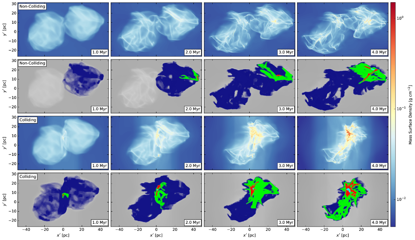
Figure 1: Row 1: Time evolution of projected mass surface density for the non-colliding model. Row 2: Connected Extractions (CEs), the largest spatially-connected sub-structures for each density threshold are shown plotted over the corresponding grayscale mass surface density map. Blue, green, red, and cyan correspond to ${\rm CE_{2}^{nc}}$, ${\rm CE_{3}^{nc}}$, ${\rm CE_{4}^{nc}}$, and ${\rm CE_{5}^{nc}}$, respectively (see text). Rows 3-4: Same as rows 1-2 except for the colliding model. Snapshots at $t=1$, 2, 3, and 4 Myr are shown. The visualizations adopt the rotated coordinate system $(x^{\prime},y^{\prime},z^{\prime})$ (i.e., the simulation coordinates $(x,y,z)$ transformed by a $(\theta,\phi)=(\timeform{15D},\timeform{15D})$ rotation used throughout this paper series.

Figure 1 shows the time evolution of the non-colliding and colliding models. For each case, maps of mass surface density, $\Sigma$, and the CEs are shown.

Evolution of the non-colliding case is dominated by the initial turbulent velocity field and self-gravity. A network of dispersed filamentary structures develops over time, with slowly increasing differentiation in mass surface density. By $t=4\>{\rm Myr}$, $\Sigma\approx 0.5\>{\rm g\>cm^{-2}}$ is seen in isolated regions. Overall evolution is relatively quiescent and the spatial extent of the original GMCs is roughly preserved.

${\rm CE_{2}^{nc}}$ contains most of the material from GMC 2 by $t=1\>{\rm Myr}$ and, by 3 Myr, encompasses both GMCs. ${\rm CE_{3}^{nc}}$ grows from a relatively isolated region near the right-most edge of GMC 2 into a structure tens of parsecs in scale by $4\>{\rm Myr}$, spanning much of GMC 2. ${\rm CE_{4}^{nc}}$ retains a highly filamentary morphology and generally occupies a small portion GMC 2. By $4\>{\rm Myr}$, it spans tens of parsecs and includes multiple filaments, with ${\rm CE_{5}^{nc}}$ having formed near a filament junction.

In contrast, the colliding case is dominated by two large-scale bulk flows which compress both the GMCs and CNM. This forms a centralized conglomeration of filamentary structures with a primarily flattened morphology oriented orthogonal to the collision axis. Secondary filaments extend outward from this region as well. Large shocks sweep up the gas in the growing collision region, eventually encompassing all material from the originally separated GMCs. Relative to the non-colliding case, the collision forms dense structures with $\Sigma>0.5\>{\rm g\>cm^{-2}}$ at much earlier times and these are predominantly clustered within the central main filament.

By $t=1\>{\rm Myr}$, the collision has bridged ${\rm CE_{2}^{c}}$ into both GMCs, and it effectively traces the total combined GMC gas throughout the simulation. Additionally, ${\rm CE_{3}^{c}}$ and ${\rm CE_{4}^{c}}$ have formed at the GMC collision interface by this time. Over the next few Myrs, ${\rm CE_{3}^{c}}$ grows to encompass most of GMC 2 and eventually the entire complex of high-density gas of the primary filament. ${\rm CE_{4}^{c}}$ and ${\rm CE_{5}^{c}}$ remain localized within the collisional interface and grow over time as additional gas is fed into the region.

3.2 Volume Density PDFs

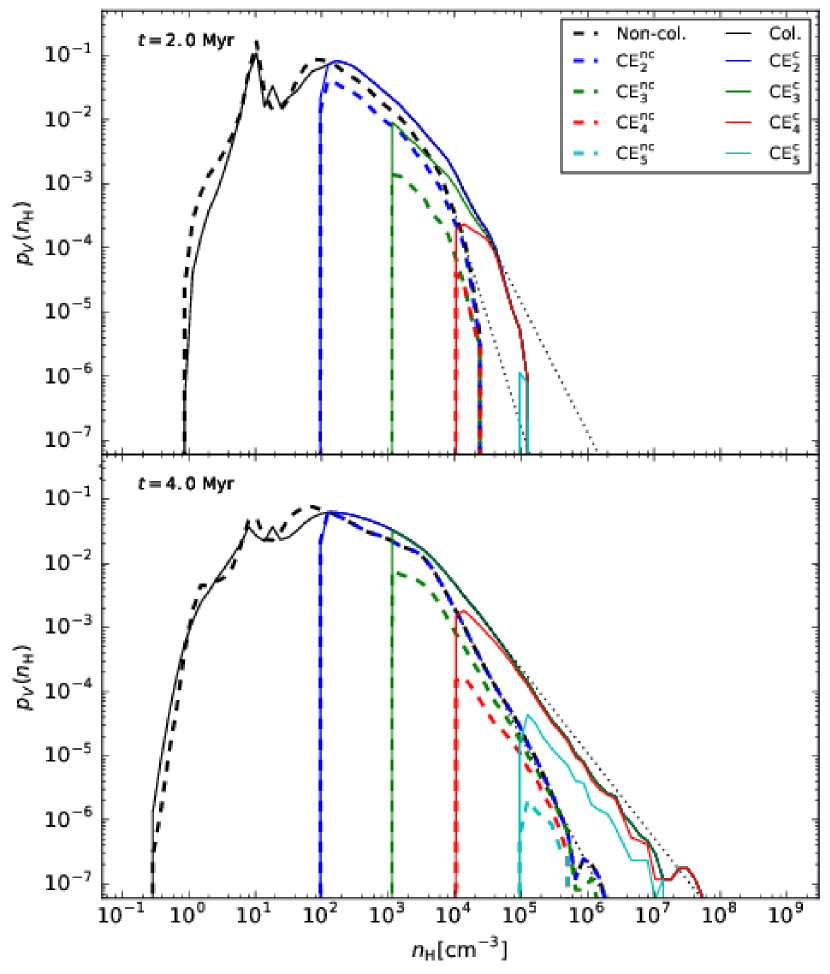
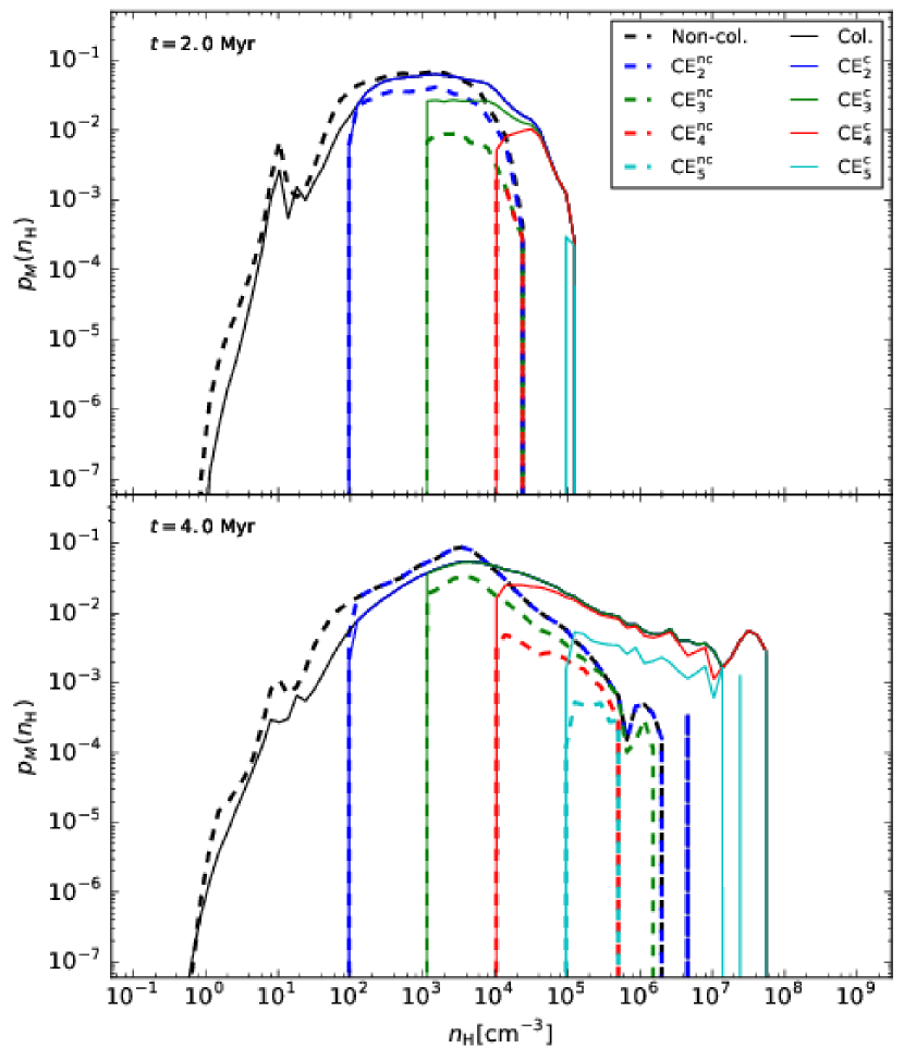
Figure 2: (Left:) Volume-weighted PDFs at $t=2$ and 4 Myr of GMC evolution are shown. PDFs for the total gas (black), ${\rm CE_{2}}$ (blue), ${\rm CE_{3}}$ (green), ${\rm CE_{4}}$ (red), and ${\rm CE_{5}}$ (cyan) are plotted. Dashed lines represent the non-colliding case, while solid lines represent the colliding case. Power laws are fit to each total gas PDF for $n_{\rm H}>10^{4}\>{\rm cm^{-3}}$. (Right:) Same as left, except for mass-weighted PDFs.

Probability distribution functions (PDFs) of gas have been used to quantify various properties of supersonic turbulence. They can be shaped by self-gravity, shocks, and magnetic fields (see, e.g., Vazquez-Semadeni, 1994; Padoan et al., 1997a, b; Kritsuk et al., 2007; Federrath et al., 2008; Price, 2012; Collins et al., 2012; Burkhart et al., 2015). A notable feature both in observations (of mass surface density, $\Sigma$) and simulations (of volume density, $\rho$) is a lognormal distribution of densities. Paper II compared $\Sigma$-PDFs with an observed Infrared Dark Cloud IRDC from Butler et al. (2014) and Lim et al. (2016) and found consistency between the observed $\Sigma$-PDF and those formed in colliding GMC simulations, though later stages ($t>4\>{\rm Myr}$) of non-colliding GMCs were not ruled out.

A lognormal PDF takes the form:

$${p_{V}(s)=\frac{1}{\sqrt{2\pi\sigma_{s}^{2}}}\exp\left(\frac{(s-\overline{s})^{2}}{2\sigma_{s}^{2}}\right)d\ln\rho},$$ (1)

where $s\equiv\ln(\rho/\rho_{0})$, and the mean ($\overline{s}$) and variance ($\sigma_{s}$) of $\ln\rho$ are related by $\overline{s}=-\sigma_{s}^{2}/2$ (Vazquez-Semadeni, 1994).

The turbulent sonic Mach number, $\mathcal{M}$, has been shown in simulations to be related to the standard deviation of the logarithm of density, $\sigma_{s}$, via

$${\sigma_{s}=\sqrt{\ln(1+b^{2}\mathcal{M}^{2})}}.$$ (2)

The constant $b$, often referred to as the turbulence driving parameter, depends on the turbulent driving modes of the acceleration field. From numerical simulations of periodic boxes of driven turbulence, $b=1/3$ for fully solenoidal (divergence-free) forcing (Padoan et al., 1997b; Kritsuk et al., 2007; Federrath et al., 2008, 2010), while $b=1$ for fully compressive (curl-free) forcing (Federrath et al., 2008, 2010).

Figure 2 shows volume-weighted and mass-weighted density PDFs at $t=2$ and 4 Myr, normalized to total gas fraction. PDFs for non-colliding and colliding clouds, along with their respective CEs are plotted together for comparison.

The volume-weighted PDFs at 2 Myr show a more broadened distribution for the colliding case. Densities have also reached an order of magnitude higher at this time, to $\sim 10^{5}\>{\rm cm^{-3}}$. The non-colliding PDF is fit with $\sigma_{s}=1.06$ and the colliding PDF, with $\sigma_{s}=1.14$. Mass-weighted sonic Mach numbers, directly calculated from the individual cell values, yield $\mathcal{M}=10.90$ for the non-colliding case and $\mathcal{M}=13.05$ for the colliding. Values of $b=0.13$ were found (i.e., relatively low values, but not indicative of any particular turbulent driving mode.) The collision also produces CEs that occupy a higher fraction of total gas at their given densities. This indicates that most of the high-density gas in a collision is contained within connected structures concentrated at the collisional interface. In the non-colliding case, high-density gas is decentralized. This trend is seen throughout all of the PDFs.

As the simulations progress to 4 Myr, the PDFs broaden in both models. They show similar behavior at low-densities, but the collision forms a higher-end tail, reaching almost two orders of magnitude greater densities, to $\sim 10^{8}\>{\rm cm^{-3}}$. These PDFs are fit with $\sigma_{s}=1.42$ for the non-colliding case and $\sigma_{s}=1.63$ for the colliding case. Notably, the Mach number for the non-colliding case has decreased to $\mathcal{M}=9.73$ while for the colliding case it has instead increased to $\mathcal{M}=15.22$. This may be indicative of the collision inducing increased turbulence into the GMC-GMC system. In this time, the turbulent driving mode $b$ has increased to 0.26 and 0.24 for the non-colliding and colliding models, respectively. We note, with caveats that our boundary conditions are not those of a periodic box and that the precise effects of the non-turbulent ambient medium are unaccounted for, our measured values of $b$ are close to those seen in purely solenoidal driving simulations. Additionally, these have increased relative to earlier times, perhaps trending toward more compressive modes as gravitational collapse begins to dominate. The similarity of $b$ measured between isolated and colliding clouds indicates that this parameter is not strongly affected by cloud collisions in our particular simulation set-up.

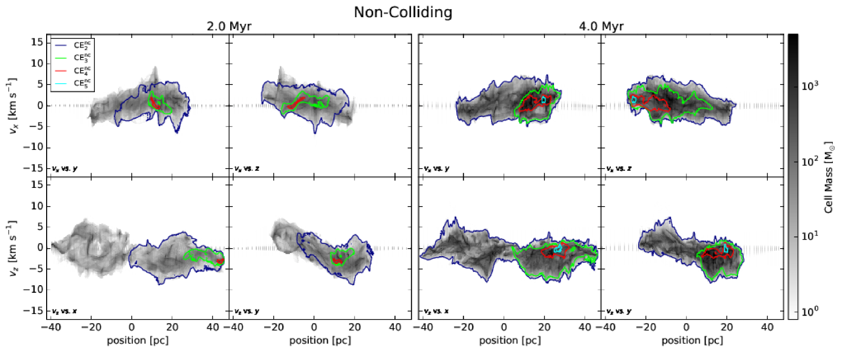
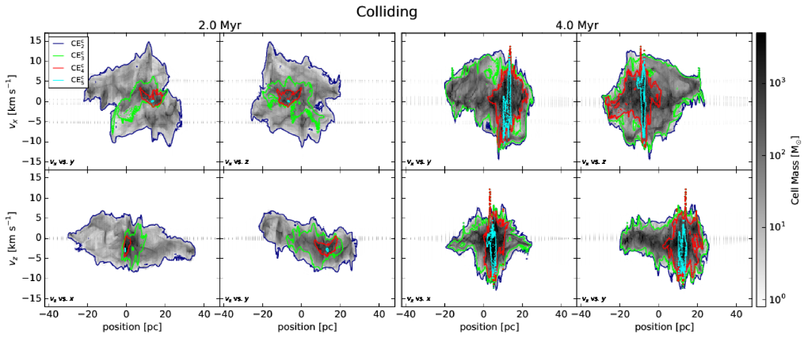
Figure 3: Position-velocity diagrams for the non-colliding (top) and colliding (bottom) models. In each model, behavior at $t=2$ (left panels) and 4 Myr (right panels) are shown. The sub-panels show line-of-sight velocities $v_{x}$ and $v_{z}$ versus orthogonal positions. The kinematic structure for the total gas is depicted as the grayscale colormap, while the CEs are denoted with correspondingly colored boundaries. The edges of the shock in the ambient medium and the associated central density enhancement can be seen in grey.

Deviations from purely lognormal PDFs at high densities in the form of power-law tails, i.e., $p(\rho)=a\rho^{-k}$, are often attributed to gravitational collapse (Klessen, 2000; Vázquez-Semadeni et al., 2008). From isothermal self-gravitating supersonic turbulence simulations, Kritsuk et al. (2011) found indices of −1.67 and −1.5 for intermediate and high density thresholds, respectively, with flattening potentially due to the onset of rotational support. Self-gravitating MHD simulations in Federrath & Klessen (2013) produced high-density tails consistent with radial density profiles of power law index $k=-1.5$ to -2.5.

We investigate power law fits to the high-density regimes ($n_{\rm H}>10^{4}\>{\rm cm^{-3}}$) of our PDFs. At 2 Myr, the non-colliding case has an index of $k=-3.35$, while the colliding case has $k=-2.03$. At 4 Myr, the indices are $k=-2.00$ and $k=-1.32$ for the non-colliding and colliding cases, respectively. In both models, the index becomes shallower as the clouds evolve, with the GMC collision expediting this process.

The mass-weighted PDFs are presented as well in Fig. 2, and emphasize differences between the non-colliding and colliding cases that grow over time. In subsequent sections, analysis of mass-weighted quantities are commonly used. These panels thus serve to more intuitively display the relative contributions of gas at different densities, particularly of the CEs.

3.3 Kinematics

3.3.1 Position-velocity diagrams

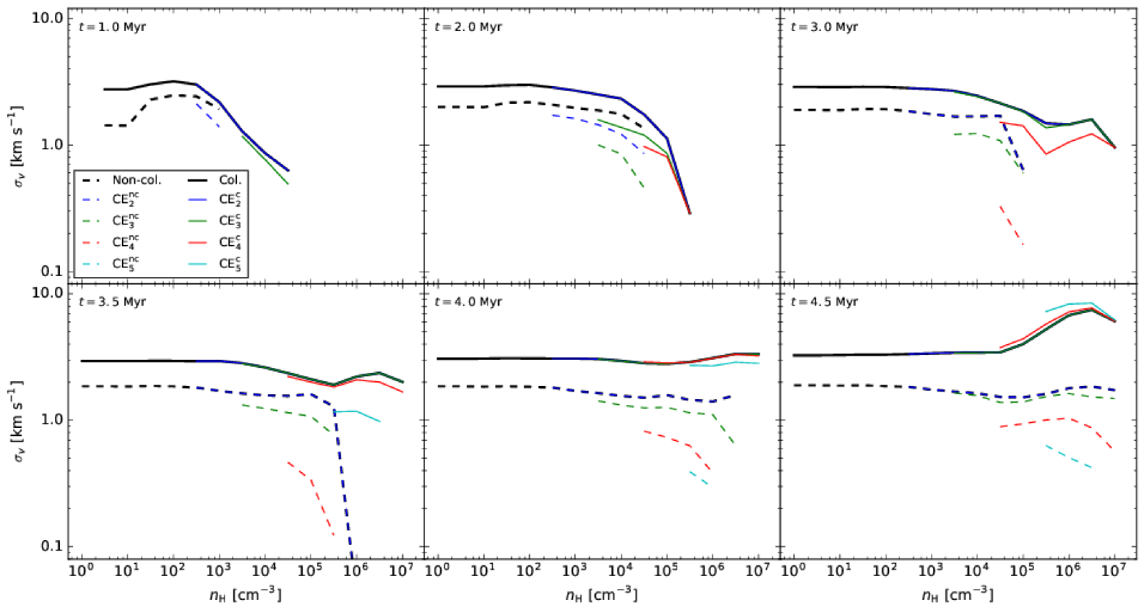
Figure 4: Velocity dispersions as functions of density. Each panel represents a different snapshot in time, from $t=1$ to 4.5 Myr. The non-colliding case is represented by dashed lines, while the colliding case is represented by solid lines. For each model, $\sigma_{v}$ (averaged over the $x$, $y$, and $z$ lines-of-sight) for the total gas content (black), $\rm{CE_{2}}$ (blue), $\rm{CE_{3}}$ (green), $\rm{CE_{4}}$ (red), and $\rm{CE_{5}}$ (cyan) is plotted.

We investigate the velocity structure of the entire clouds and individual CEs via position-velocity ($p-v$) diagrams. Observationally, this method is used to determine velocity dispersion and velocity gradients of GMCs and IRDCs (e.g., Hernandez & Tan, 2015). Paper II investigated $p-v$ diagrams using synthetic ${}^{13}{\rm CO}$-connected structures and found velocity dispersions in colliding GMC simulations were higher than those of non-colliding clouds by a factor of a few and were in agreement with observed velocity dispersions of $\sim$ few ${\rm km\>s^{-1}}$ (Hernandez & Tan, 2015).

Figure 3 shows $p-v$ diagrams of the gas density in the non-colliding and colliding simulations, measured along lines of sight for the collision axis ($v_{x}$) and for a side view ($v_{z}$). Results for $v_{y}$ are not displayed, but are in general similar to those along $v_{z}$.

In the non-colliding model at 2 Myr, the overall gas distribution shows turbulent kinematic structures that are generally within $\pm 5\>{\rm km\>s^{-1}}$. The individual GMCs can be distinguished in the $x$ direction. ${\rm CE_{2}^{nc}}$, which traces GMC 2 at this time (see Section 3.1), shows similar kinematic structure. ${\rm CE_{3}^{nc}}$ and ${\rm CE_{4}^{nc}}$ can also be seen, with relatively narrow velocity spreads of at most a few ${\rm km\>s^{-1}}$.

At 2 Myr, the colliding model has formed a more spatially compact structure and exhibits much stronger kinematic signatures. Portions of the GMCs exceed $\pm 10\>{\rm km\>s^{-1}}$, due to the bulk flow velocity combined with initially turbulent gas. This gas has not yet interacted with the incoming GMC. ${\rm CE_{2}^{c}}$, which contains the combined GMC gas, shows more disrupted structures with high velocity dispersions. The cloud collision can be clearly seen in the $v_{x}$ vs. $y$ and $v_{x}$ vs. $z$ panels, with two large, opposing velocity components bridged by an overdense intermediate-velocity region. It is within this collisional interface that the primary higher-density structures–${\rm CE_{3}^{c}}$, ${\rm CE_{4}^{c}}$, and ${\rm CE_{5}^{c}}$–form. Compared with the non-colliding model, the velocity dispersion is much higher, although ${\rm CE^{c}}$s at successively higher densities similarly form with lower relative velocity dispersions. The cloud collision is less apparent along $v_{z}$, but higher velocity dispersions relative to the non-colliding case can be seen at the interface.

At 4 Myr, $p-v$ diagrams for the non-colliding model reveal the presence of higher density structures via the total projected cell mass values, but overall velocity dispersion is similar. ${\rm CE_{2}^{nc}}$ now includes both GMCs, and ${\rm CE_{3}^{nc}}$ tracks the majority of GMC 2. ${\rm CE_{4}^{nc}}$ and ${\rm CE_{5}^{nc}}$, which have now formed, contain gas with relatively low velocity dispersions.

The colliding case at 4 Myr reveals very different behavior, exhibiting much higher velocities and more compact gas structures. CEs at this stage of evolution now include gas with much higher velocity dispersions, with higher-density CEs showing large amounts of disruption. Compared to the colliding case at 2 Myr, the gas kinematics are now dominated by post-collisional gas located in the central structure rather than the pre-collisional gas from the original GMCs.

3.3.2 Velocity dispersion

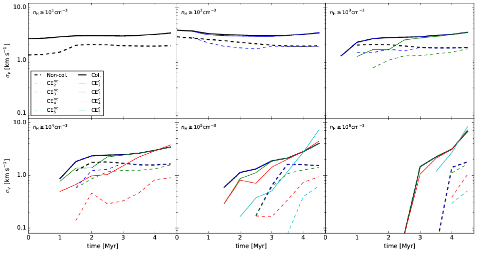
Figure 5: Velocity dispersion as a function of time. Each panel displays the time evolution of gas above a certain density threshold, from $n_{\rm H}=10$ to $10^{6}\>{\rm cm^{-3}}$. The non-colliding case is represented by dashed lines, while the colliding case is represented by solid lines. For each model, $\sigma_{v}$ (averaged over the $x$, $y$, and $z$ lines-of-sight) for the total gas content (black), $\rm{CE_{2}}$ (blue), $\rm{CE_{3}}$ (green), $\rm{CE_{4}}$ (red), and $\rm{CE_{5}}$ (cyan) is plotted.

To understand the evolution of GMC kinematics in greater detail, we analyze the velocity dispersion, $\sigma_{v}$, both as functions of density (Figure 4) and time (Figure 5). $\sigma_{v}$ is calculated as the cumulative mass-weighted gas velocity dispersion, taking the average of the $x$, $y$, and $z$ lines of sight. For the non-colliding model, the components $\sigma_{v,x}$, $\sigma_{v,y}$, and $\sigma_{v,z}$ (not shown), are fairly similar throughout their evolution. In the colliding model, $\sigma_{v,x}$ is initially larger, but the dispersions in fact converge by $\sim 2-3\>{\rm Myr}$ after the GMCs have sufficiently interacted.

In Figure 4, $\sigma_{v}$ versus $n_{\rm H}$ is plotted at various snapshots in time. $\sigma_{v}$ for the total gas and in CEs above given $n_{\rm H}$ thresholds are shown. The top row, showing $t=1$, 2, and 3 Myr outputs, follows a similar trend in both the non-colliding and colliding models. As the GMCs evolve, the $\sigma_{v}$ versus $n_{\rm H}$ relation reveals the formation of higher density gas, with the colliding case exhibiting relatively higher $\sigma_{v}$ throughout the entire density range due to the bulk flows. In both models, $\sigma_{v}$ versus $n_{\rm H}$ remains fairly constant (i.e., a few ${\rm km\>s^{-1}}$) before dropping off at higher $n_{\rm H}$. Additionally, overall lower $\sigma_{v}$ values are measured in increasingly denser CEs. At these earlier times, the $\sigma_{v}$ at a given density is highest in the total gas, revealing higher relative dispersions between sub-structures than within sub-structures.

After $t\approx 3\>{\rm Myr}$, this trend begins to shift, especially in the colliding model. The GMC collision induces higher $\sigma_{v}$ for even the highest density gas. Higher-density ${\rm CE^{c}}$s begin to have larger relative $\sigma_{v}$ as well. At 4 Myr, $\sigma_{v}$ within $\rm{CE_{2}^{c}}$, $\rm{CE_{3}^{c}}$, and $\rm{CE_{4}^{c}}$ match that of the overall gas, while $\rm{CE_{5}^{c}}$ has only slightly lower $\sigma_{v}$. By 4.5 Myr, $\sigma_{v}$ for the highest-density CEs actually exceed that of the containing CEs and overall gas, indicating transition to a higher velocity dispersion within dense structures versus between structures. Conversely in the non-colliding model, the behavior at early times remains, with lower $\sigma_{v}$ measured for higher-density CEs.

Offner et al. (2008) found in driven and decaying turbulent box simulations that turbulence driving produced structures with velocity dispersions similar or slightly higher in value within the densest regions (proto-stellar cores/clumps) compared to the core-to-core dispersion. A sign of turbulent decay was that velocity dispersions within cores sharply increased with density after a free-fall time.

Figure 5 follows the time evolution of $\sigma_{v}$ for the total gas and in each CE. Different panels correspond to increasing gas density thresholds, above which $\sigma_{v}$ is calculated. Only CEs at the relevant density threshold are plotted. However, $\sigma_{v}$ versus $t$ for a given CE differs from panel to panel based on the density threshold. For example, consider $\rm{CE_{4}^{c}}$ in the $n_{\rm H}\geq 10^{5}\>{\rm cm^{-3}}$ panel (bottom center). The line associated with $\rm{CE_{4}^{c}}$ shows the velocity dispersion for all gas $\geq 10^{5}\>{\rm cm^{-3}}$ within $\rm{CE_{4}^{c}}$, which includes $\rm{CE_{5}^{c}}$ as well as other dense structures. Such values can be used to compare overall dispersion not limited to a single CE.

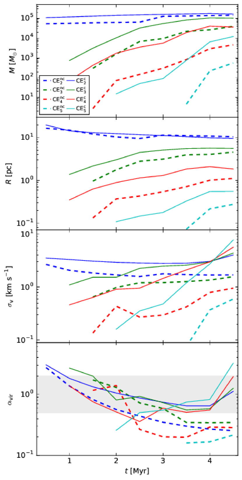
Figure 6: Virial analysis. (From top to bottom:) time evolution of total mass, half-mass radii, mean 1D velocity dispersion, and corresponding virial parameter. The non-colliding and colliding models are plotted as dashed and solid lines, respectively. Values for respective CEs are shown in blue (${\rm CE_{2}}$), green (${\rm CE_{3}}$), red (${\rm CE_{4}}$), and cyan (${\rm CE_{5}}$).

The evolution of $\sigma_{v}$ for gas at lower-density thresholds (top row) stays fairly constant at $\sim 3\>{\rm km\>s^{-1}}$ for the total gas, $\rm{CE_{2}}$, and $\rm{CE_{3}}$ in both non-colliding and colliding models. For all thresholds and all extractions, the colliding model produces higher $\sigma_{v}$ than the non-colliding model by at least a factor of $\sim 2$.

For the $n_{\rm H}\geq 10^{4}\>{\rm cm^{-3}}$ threshold and higher, the time evolution shows generally increasing $\sigma_{v}$. For higher density thresholds, $\sigma_{v}$ rises at a faster rate. $t=4\>{\rm Myr}$ can be seen as the critical time in the colliding case where $\sigma_{v}$ within structures exceeds that found overall. At this time, all CEs are measured to have $\sigma_{v}\approx 3\>{\rm km\>s^{-1}}$. Structures formed in the non-colliding model have a wide range of $\sigma_{v}$, from $\sim 1.5\>{\rm km\>s^{-1}}$ for $\rm{CE^{nc}_{2}}$ down to $\sim 0.4\>{\rm km\>s^{-1}}$ for $\rm{CE^{nc}_{5}}$.

3.4 Dynamics

Dynamical properties of gas structures can be described via a virial analysis, which calculates the relative importance of a cloud’s internal kinetic energy to self-gravity. This ratio of these energies is defined as the virial parameter,

$$\alpha_{\rm vir}=\frac{5\sigma R}{GM},$$ (3)

where $\sigma$ is the line-of-sight velocity dispersion, $R$ is the radius, and $M$ is the total mass of the structure. A uniform sphere in virial equilibrium has $\alpha_{\rm vir}=1$. Note, values of $\alpha_{\rm vir}<2$ still imply a gravitationally bound structure if magnetic and surface pressure terms are ignored (Bertoldi & McKee, 1992). Virial analysis of a cloud may reveal signatures of its kinematic history and thus can be a useful diagnostic to understand dense gas formation triggered by GMC collisions. For example, a collision and merger of two clouds would be expected to raise the virial parameter of the combined structure, depending on how it is defined.

Figure 6 displays the virial parameter and component properties measured for each CE. Values for mass, radius, velocity dispersion, and virial parameter are calculated for CEs in the non-colliding and colliding GMC models.

In both models, the total masses of the CEs generally increase monotonically with time, as the extractions accrete surrounding gas and join with other structures. ${\rm CE_{2}}$ masses formed in the collision are only slightly greater than those in the non-colliding case, as they track the initial GMC material. For higher density CEs, the relative difference grows up to factors of a few tens. Overall, the colliding case forms higher density CEs at approximately 0.5 to 1 Myr earlier times, with greater total masses.

The radius of a given CE is defined as the spherical radius calculated from the mean CE gas density. The radii of ${\rm CE_{2}}$s decrease gradually as the GMCs contract gravitationally, while the higher-density CEs increase in size as additional material is included. While the non-colliding model retains a slightly larger measured radius relative to the compressed GMCs, the collision forms larger higher-density structures.

Larger differences are seen in velocity disperison, described in detail in Section 3.3.2. Structures in the non-colliding model have $\sigma_{v}$ that increase slowly with time throughout the early evolution, with denser CEs exhibiting lower $\sigma_{v}$ for the entirety of the simulation For colliding GMCs, structures with much larger velocity dispersions are found. During early stages of evolution, values of $\sigma_{v}$ are a factor of a few times higher due to the contributions of the converging flows. The velocity dispersion increases at a more rapid pace for higher-density CEs, with $\sigma_{v}$ for all CEs converging to roughly $3\>{\rm km\>s^{-1}}$ at $4\>{\rm Myr}$. After this time, the highest density CEs have higher velocity dispersions.

The combined influence of these parameters leads to notable differences in the resulting virial parameter. In both models, the GMCs are initialized with moderately supervirial turbulence, which then naturally decays, as indicated by the initial ${\rm CE_{2}}$s. In the non-colliding case, the virial parameters of the ${\rm CE^{nc}}$s decrease to sub-virial states by $t\sim 3\>{\rm Myr}$ and remain so for the remainder of the simulation. Higher-density ${\rm CE^{nc}}$s are measured with lower $\alpha_{\rm vir}$, and all ${\rm CE^{nc}}$s reach $\alpha_{\rm vir}\simeq 0.2-0.4$ by $t=3.5\>{\rm Myr}$ and remain fairly constant. Note the presence of large-scale $B$-fields can help stabilize these structures. The structures formed in the colliding GMCs have measured virial parameters higher in general by a factor of a few, and remain near the $\alpha_{\rm vir}\simeq 0.5-2$ range from their formation to the end of the simulation. Higher-density ${\rm CE^{c}}$s have higher $\alpha_{\rm vir}$–opposite of the trend seen in the non-colliding case. The virial parameters of all ${\rm CE^{c}}$s show growth after 4 Myr, dominated by the increase in $\sigma_{v}$.

Observationally, Hernandez & Tan (2015) measured $\alpha_{\rm vir}\sim 1$ for 10 IRDCs/GMCs (with dispersion of about a factor of 2) and found that gas in IRDCs had moderately enhanced velocity dispersions and virial parameters relative to GMCs, which may be indicative of more disturbed gas kinematics particularly in denser regions. This is consistent with dense gas structures formed from our numerical simulations of GMC collisions.

3.5 Turbulent Momentum

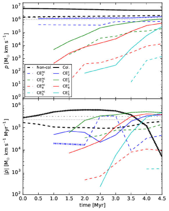
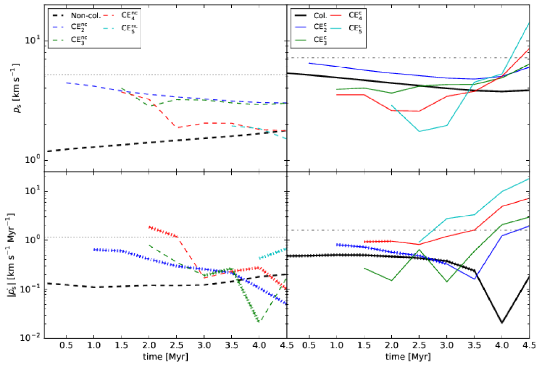
Figure 7: (Left:) Time evolution of turbulent momentum (top) and the magnitude of its time derivative (bottom), with hatched segments denoting negative values. Total momentum is calculated for all gas and individual CEs in the simulation frame. The non-colliding case is drawn with dashed lines while the colliding case is drawn with solid lines. For each plot, the grey horizontal lines indicate the expected initial values for $p$ and the expected average $\dot{p}$ over 4.5 Myr for material contained within the non-colliding GMCs (dotted) and colliding GMCs (dash-dot), respectively. (Right:) Time evolution of specific turbulent momentum (top), $p_{\rm s}$, normalized to the total mass of the structure. The absolute value of its time derivative (bottom), $|\dot{p}_{\rm s}|$ is also plotted, with hatched segments denoting negative values. Non-colliding and colliding models are shown as dashed and solid lines in separate columns, respectively, with the expected GMC initial values in gray.

The injection of turbulence from cloud collisions has been investigated on galactic scales (Tan et al., 2013; Jin et al., 2017; Li et al., 2017). From hydrodynamic simulations of flat rotation curve galactic disks, Li et al. (2017) found that GMC collisions occurred primarily with mass ratios only moderately less than 1, relative velocities of $\sim$10s of ${\rm km\>s^{-1}}$, and timescales between subsequent collisions of $\sim 10$ to $20\>{\rm Myr}$ for conditions near a galactocentric radius of $r\sim 4~{}{\rm kpc}$.

The average rate of “internal turbulent momentum” injection per GMC, $\dot{p}_{\rm CC}$, is expressed as

$$\dot{p}_{\rm CC}=\frac{M_{\rm GMC}v_{\rm rel}}{t_{\rm col}}$$ (4)

where $M_{\rm GMC}$ is the GMC mass, $v_{\rm rel}$ is the relative collision velocity, and $t_{\rm col}$ is the average time between collisions. Using the GMC collision parameters from Li et al. (2017) described above, $\dot{p}\sim 10\times 10^{5}~{}M_{\odot}{\rm\>km\>s^{-1}\>Myr^{-1}}$. Further, by balancing the total injection and dissipation of turbulent momentum leads to estimation of average GMC mass surface densities of $\Sigma_{\rm GMC,eq}\simeq 100\>M_{\odot}{\rm\>pc^{2}}$, consistent with observations.

Figure 7 shows the time evolution for turbulent momentum, $p$ (top) and the absolute value of its time derivative, $|\dot{p}|$ (bottom). $p$ is calculated as the magnitude of the total momentum for a given region, i.e., $p=\int_{V}{\rho|v|dV}$, a scalar quantity, with velocities calculated in the simulation frame. $|\dot{p}|$ accounts for the total turbulent momentum injection as well as advection into the CE. The total momenta and rates are shown on the left, while quantities for the specific momentum $p_{\rm s}$, i.e., normalized to the mass of the region or CE, are displayed on the right. Values for the total gas and all CEs are calculated for both the non-colliding and colliding models. Also shown are horizontal lines displaying the expected initial value of $p$ for the two GMCs in non-colliding and colliding models. The former accounts for the initial velocity dispersion of the GMC gas while the latter includes terms for the bulk colliding flows. Dividing the total 4.5 Myr gives the expected average rate, $\dot{p}$. By comparing CEs with this initial value, we can estimate the efficiency of the conversion of turbulent momentum into denser structures.

For the total and ${\rm CE_{2}}$ gas, $p$ remains fairly constant over time, while higher-density CEs experience monotonic increases. $p$ in ${\rm CE^{nc}}$s are in general smaller than in ${\rm CE^{c}}$s by up to a few orders of magnitude. Denser sub-regions have necessarily smaller $p$ but experience larger relative growth which can be attributed to mass advection and, in primarily colliding cases, increased velocity dispersion. The ${\rm CE_{2}}$s, once both GMCs are taken into account, closely agree with the analytic expected initial values for $p$ within the GMC gas.

The rate at which this momentum is injected into the various structures, $\dot{p}$, is also calculated. The non-colliding simulation domain is shown to have slightly positive growth of turbulent momentum as material flows into the volume. The colliding case shows negative values of $\dot{p}$, indicated by the hatched lines, due to the lower velocity post-shocked ambient gas. The individual CEs all exhibit positive $\dot{p}$ by 2 Myr, with ${\rm CE^{nc}}$s having generally lower rates ranging widely from $10^{3}-10^{5}~{}{\rm M_{\odot}\>km\>s^{-1}\>Myr^{-1}}$ and ${\rm CE^{c}}$s converging near $4\times 10^{5}~{}{\rm M_{\odot}\>km\>s^{-1}\>Myr^{-1}}$. Values for $\dot{p}$ for ${\rm CE^{c}_{2}}$ grow to those consistent with Equation 4, while ${\rm CE^{nc}_{2}}$ is generally an order of magnitude lower.

To minimize the effects of mass advection into the structure, we investigate the specific momentum, $p_{\rm s}$, for each region. For the non-colliding model, $p_{\rm s}$ gradually increases for overall gas but slowly decreases for all ${\rm CE^{nc}}$s. This illustrates overall decay of turbulent momentum due to decay of turbulence, though short-lived generation due to the collapse and attraction of the clouds occurs. $p_{\rm s}$ of a few ${\rm km\>s^{-1}}$ are seen in this case. This general decrease is shown by ${\rm CE^{nc}}$s with $\dot{p}_{\rm s}\approx-0.1{\rm km\>s^{-1}\>Myr^{-1}}$.

The $p_{\rm s}$ in the colliding GMC case decreases for overall gas as well as for ${\rm CE^{c}_{2}}$ initially. However, later stages and higher-density ${\rm CE^{c}}$s have $p_{\rm s}$ of $\sim 10~{}{\rm km\>s^{-1}}$. Comparisons with the expected $p_{\rm s}$ show approximate turbulent momentum injection efficiencies of $\sim 0.7-0.8$ into ${\rm CE^{c}_{2}}$ for the majority of the simulation and initially smaller efficiencies for higher-density ${\rm CE^{c}}$s, but increasing over time. The rates fluctuate as the collision occurs, but at later times results in ${\rm CE^{c}_{2}}$ near $\dot{p}_{\rm s}\approx 1{\rm km\>s^{-1}\>Myr^{-1}}$ and increased values for higher-density ${\rm CE^{c}}$s. In contrast to the non-colliding case, turbulent momenta grows positively in all the ${\rm CE^{c}}$s.

4 Discussion and Conclusions

We have analyzed three-dimensional turbulent MHD simulations of non-colliding and colliding GMCs in order to investigate properties of turbulence from GMC to clump scales and to determine whether or not GMC collisions can be a source of supersonic turbulent momentum injection. Properties of the global gas and that which is contained within increasingly dense, spatially-connected structures (CEs) are compared. The morphology, volume density PDFs, velocity dispersion, virial analysis, and rate of injection of turbulent momenta are discussed.

The density PDFs reveal relatively smaller values of $\sigma$ in the non-colliding case compared with the GMC collision. The collision produces gas which is more highly turbulent, with $\mathcal{M}\sim 13$ and increasing with time, while the more quiescent model has $\mathcal{M}\sim 9$ and is decaying.

Velocity dispersions found in the total gas and especially within CE structures were consistently higher in the colliding scenario. Key differences occur as the models evolve: in the colliding case, high levels of velocity dispersion are maintained even at high densities overall, whereas the non-colliding case forms high-density gas with low velocity dispersions. At late stages, high-density ${\rm CE^{c}}$s have greater velocity dispersion than the low-density ${\rm CE^{c}}$s. In the non-colliding case, the opposite trend occurs.

The virial parameter is also generally lower in the non-colliding case, quickly decreasing and remaining at sub-virial states through the course of the simulation. Note, however, that some support of the structures is expected to be derived from the presence of large-scale $B$-fields in the clouds. The GMC collision, on the other hand, forms approximately virialized dense gas structures that persist even into the late stages.

The rate of turbulent momentum injection, $\dot{p}$, was found to be consistent with a simple model based on the initial global momenta of the colliding clouds. This implies relatively high conversion efficiencies of the bulk momenta of the collision into internal turbulence. These results lend support to a model of maintenance of GMC internal turbulence via GMC-GMC collisions that has been investigated in simulations of shearing galactic disks by Li et al. (2017). We also note that the colliding GMCs produced greater rates of specific turbulent momentum injection in higher density structures whereas the non-colliding GMCs experienced decreasing specific turbulent momentum.

In conclusion, parameters used to measure turbulence within dense gas indicate that GMC collisions can indeed create and maintain states of higher turbulence within dense gas structures. These are consistent with various observations of dense IRDCs. Non-colliding GMCs, on the other hand, experience turbulent decay with much less energetic high-density structures.

Computations described in this work were performed using the publicly-available Enzo code (http://enzo-project.org). This research also made use of the yt-project (http://yt-project.org), a toolkit for analyzing and visualizing quantitative data (Turk et al., 2011). The authors acknowledge University of Florida Research Computing (www.rc.ufl.edu) and the Center for Computational Astrophysics (http://www.cfca.nao.ac.jp/) for providing computational resources and support that have contributed to the research results reported in this publication. The authors thank the anonymous referee, whose comments helped to improve the article. BW acknowledges the JSPS Postdoctoral Fellowship (short-term) for its support.

References

- Bertoldi & McKee (1992) Bertoldi, F., & McKee, C. F. 1992, ApJ, 395, 140
- Bisbas et al. (2017) Bisbas, T. G., Tanaka, K. E. I., Tan, J. C., Wu, B., & Nakamura, F. 2017, ArXiv e-prints, arXiv:1706.07006
- Bryan et al. (2014) Bryan, G. L., Norman, M. L., O’Shea, B. W., et al. 2014, ApJS, 211, 19
- Burkhart et al. (2015) Burkhart, B., Collins, D. C., & Lazarian, A. 2015, ApJ, 808, 48
- Butler et al. (2014) Butler, M. J., Tan, J. C., & Kainulainen, J. 2014, ApJ, 782, L30
- Christie et al. (2017) Christie, D., Wu, B., & Tan, J. C. 2017, ArXiv e-prints, arXiv:1706.07032
- Collins et al. (2012) Collins, D. C., Kritsuk, A. G., Padoan, P., et al. 2012, ApJ, 750, 13
- Dedner et al. (2002) Dedner, A., Kemm, F., Kröner, D., et al. 2002, Journal of Computational Physics, 175, 645
- Dobbs (2008) Dobbs, C. L. 2008, MNRAS, 391, 844
- Dobbs et al. (2015) Dobbs, C. L., Pringle, J. E., & Duarte-Cabral, A. 2015, MNRAS, 446, 3608
- Duarte-Cabral et al. (2011) Duarte-Cabral, A., Dobbs, C. L., Peretto, N., & Fuller, G. A. 2011, A&A, 528, A50
- Federrath & Klessen (2012) Federrath, C., & Klessen, R. S. 2012, ApJ, 761, 156
- Federrath & Klessen (2013) —. 2013, ApJ, 763, 51
- Federrath et al. (2008) Federrath, C., Klessen, R. S., & Schmidt, W. 2008, ApJ, 688, L79
- Federrath et al. (2010) Federrath, C., Roman-Duval, J., Klessen, R. S., Schmidt, W., & Mac Low, M.-M. 2010, A&A, 512, A81
- Federrath et al. (2011) Federrath, C., Sur, S., Schleicher, D. R. G., Banerjee, R., & Klessen, R. S. 2011, ApJ, 731, 62
- Fujimoto et al. (2014) Fujimoto, Y., Tasker, E. J., & Habe, A. 2014, MNRAS, 445, L65
- Fukui et al. (2014) Fukui, Y., Ohama, A., Hanaoka, N., et al. 2014, ApJ, 780, 36
- Gammie et al. (1991) Gammie, C. F., Ostriker, J. P., & Jog, C. J. 1991, ApJ, 378, 565
- Goldbaum et al. (2011) Goldbaum, N. J., Krumholz, M. R., Matzner, C. D., & McKee, C. F. 2011, ApJ, 738, 101
- Hernandez & Tan (2015) Hernandez, A. K., & Tan, J. C. 2015, ApJ, 809, 154
- Jin et al. (2017) Jin, K., Salim, D. M., Federrath, C., et al. 2017, MNRAS, 469, 383
- Joung & Mac Low (2006) Joung, M. K. R., & Mac Low, M.-M. 2006, ApJ, 653, 1266
- Kennicutt (1998) Kennicutt, Jr., R. C. 1998, ApJ, 498, 541
- Klessen (2000) Klessen, R. S. 2000, ApJ, 535, 869
- Körtgen et al. (2016) Körtgen, B., Seifried, D., Banerjee, R., Vázquez-Semadeni, E., & Zamora-Avilés, M. 2016, MNRAS, 459, 3460
- Kritsuk et al. (2007) Kritsuk, A. G., Norman, M. L., Padoan, P., & Wagner, R. 2007, ApJ, 665, 416
- Kritsuk et al. (2011) Kritsuk, A. G., Norman, M. L., & Wagner, R. 2011, ApJ, 727, L20
- Larson (1981) Larson, R. B. 1981, MNRAS, 194, 809
- Leroy et al. (2008) Leroy, A. K., Walter, F., Brinks, E., et al. 2008, AJ, 136, 2782
- Li et al. (2017) Li, Q., Tan, J. C., Christie, D., Bisbas, T. G., & Wu, B. 2017, ArXiv e-prints, arXiv:1706.03764
- Lim et al. (2016) Lim, W., Tan, J. C., Kainulainen, J., Ma, B., & Butler, M. J. 2016, ArXiv e-prints, arXiv:1605.09320
- Loren (1976) Loren, R. B. 1976, ApJ, 209, 466
- Mac Low (1999) Mac Low, M.-M. 1999, ApJ, 524, 169
- Mac Low et al. (1998) Mac Low, M.-M., Klessen, R. S., Burkert, A., & Smith, M. D. 1998, Physical Review Letters, 80, 2754
- McKee & Ostriker (2007) McKee, C. F., & Ostriker, E. C. 2007, ARA&A, 45, 565
- Offner et al. (2008) Offner, S. S. R., Klein, R. I., & McKee, C. F. 2008, ApJ, 686, 1174
- Padoan et al. (2014) Padoan, P., Federrath, C., Chabrier, G., et al. 2014, Protostars and Planets VI, 77
- Padoan et al. (1997a) Padoan, P., Jones, B. J. T., & Nordlund, Å. P. 1997a, ApJ, 474, 730
- Padoan et al. (1997b) Padoan, P., Nordlund, A., & Jones, B. J. T. 1997b, MNRAS, 288, 145
- Price (2012) Price, D. J. 2012, MNRAS, 420, L33
- Scoville et al. (1986) Scoville, N. Z., Sanders, D. B., & Clemens, D. P. 1986, ApJ, 310, L77
- Stone et al. (1998) Stone, J. M., Ostriker, E. C., & Gammie, C. F. 1998, ApJ, 508, L99
- Suwannajak et al. (2014) Suwannajak, C., Tan, J. C., & Leroy, A. K. 2014, ApJ, 787, 68
- Tan (2000) Tan, J. C. 2000, ApJ, 536, 173
- Tan et al. (2013) Tan, J. C., Shaske, S. N., & Van Loo, S. 2013, in IAU Symposium, Vol. 292, IAU Symposium, ed. T. Wong & J. Ott, 19–28
- Tasker & Tan (2009) Tasker, E. J., & Tan, J. C. 2009, ApJ, 700, 358
- Truelove et al. (1997) Truelove, J. K., Klein, R. I., McKee, C. F., et al. 1997, ApJ, 489, L179
- Turk et al. (2011) Turk, M. J., Smith, B. D., Oishi, J. S., et al. 2011, ApJS, 192, 9
- van Leer (1977) van Leer, B. 1977, Journal of Computational Physics, 23, 276
- Vazquez-Semadeni (1994) Vazquez-Semadeni, E. 1994, ApJ, 423, 681
- Vázquez-Semadeni et al. (2008) Vázquez-Semadeni, E., González, R. F., Ballesteros-Paredes, J., Gazol, A., & Kim, J. 2008, MNRAS, 390, 769
- Wang & Abel (2008) Wang, P., & Abel, T. 2008, ApJ, 672, 752
- Wu et al. (2017b) Wu, B., Tan, J. C., Christie, D., et al. 2017b, ApJ, 841, 88
- Wu et al. (2017a) Wu, B., Tan, J. C., Nakamura, F., et al. 2017a, ApJ, 835, 137
- Wu et al. (2015) Wu, B., Van Loo, S., Tan, J. C., & Bruderer, S. 2015, ApJ, 811, 56