Growing a ‘Cosmic Beast’: Observations and Simulations of MACS J0717.5+3745
Abstract
We present a gravitational lensing and X-ray analysis of a massive galaxy cluster and its surroundings. The core of MACS J0717.5+3745 ( , =) is already known to contain four merging components. We show that this is surrounded by at least seven additional substructures with masses ranging from , at projected radii to Mpc. We compare MACS J0717 to mock lensing and X-ray observations of similarly rich clusters in cosmological simulations. The low gas fraction of substructures predicted by simulations turns out to match our observed values of –. Comparing our data to three similar simulated halos, we infer a typical growth rate and substructure infall velocity. That suggests MACS J0717 could evolve into a system similar to, but more massive than, Abell 2744 by , and into a supercluster by . The radial distribution of infalling substructure suggests that merger events are strongly episodic; however we find that the smooth accretion of surrounding material remains the main source of mass growth even for such massive clusters.
keywords:
Gravitational Lensing – Galaxy Clusters – Individual (MACSJ0717.5+3745)1 Introduction
Massive galaxy clusters are the most massive gravitationally bound structures in the present Universe, having grown by repeatedly accreting smaller clusters and groups (e.g. Fakhouri & Ma, 2008; Genel et al., 2010). However, most of the mass in the Universe is located outside gravitationally-bound halos. Clusters reside at the vertices of a cosmic network of large-scale filaments (Bond et al., 1996). Numerical simulations predict these filaments contain as much as half of the Universe’s baryons (Cen & Ostriker, 1999; Davé et al., 2001) in the form of a warm plasma (Fang et al., 2002; Fang et al., 2007; Kaastra et al., 2006; Rasmussen, 2007; Galeazzi et al., 2009; Williams et al., 2010; Eckert et al., 2015), and the majority of of the Universe’s dark matter (Aragón-Calvo et al., 2010).
Filaments are the scaffolding inside which clusters are built. They control the evolution of clusters. Particularly in the outskirts of a galaxy cluster, filaments create preferred directions for the accretion of smaller halos, affecting the growth and shape of the main halo. Filaments also channel infalling galaxies, accelerating or ‘pre-processing’ their morphological and stellar evolution. Substructures in filaments bias cluster mass measurements, especially from weak gravitational lensing (Martinet et al., 2016). Mis-calibrating cluster number counts can bias cosmological constraints (Martinet et al., 2016), and mis-calibrating clusters’ magnification of background galaxies can bias high-redshift galaxy number counts by up to 30% (Acebron et al., 2017). For all these reasons, observationally assessing substructures is essential if cluster evolution is to be understood and exploited.
One of the most efficient ways of mapping a distribution of mass dominated by dark matter is gravitational lensing: the bending of light from a background source as it passes near a foreground mass (for reviews see Massey et al., 2010; Kneib & Natarajan, 2011; Hoekstra et al., 2013). Gravitational lensing is a purely geometrical effect, and is thus insensitive to the dynamical state of the cluster. It has been used extensively to probe the matter distribution in and around galaxy clusters (e.g. Kneib et al., 2003; Clowe et al., 2004, 2006; Bradac et al., 2006; Limousin et al., 2007; Richard et al., 2011; Zitrin et al., 2011; Harvey et al., 2015; Massey et al., 2015; Jauzac et al., 2016; Natarajan et al., 2017; Chirivì et al., 2017). Additionally, observations of X-ray emission from infalling structures reveal the presence of hot gas – which, if virialized, is also an unambiguous signature of an underlying dark-matter halo (Neumann et al., 2001; Randall et al., 2008; Eckert et al., 2014, 2017; De Grandi et al., 2016; Ichinohe et al., 2015). The combination of lensing and X-ray information is thus a powerful tool to study the processes governing the growth of massive galaxy clusters.
The Hubble Space Telescope (HST) has recently obtained the deepest ever images of galaxy clusters, through the Hubble Frontier Fields programme (HFF; Lotz et al., 2017). This targets six of the most massive clusters in the observable Universe, which we call ‘cosmic beasts’ because of their impressive size (). These objects are rare but, as extrema, are also ideal tests of the cosmological paradigm.
One HFF galaxy cluster, Abell 2744, has been the source of recent debate. At redshift , it has a complex distribution of substructure in its core, and three filaments containing both dark matter and gas (Eckert et al., 2015). Jauzac et al. (2016) recorded a total of seven mass substructures, projected within Mpc of the cluster centre. Searching in the Illustris simulation volume (Vogelsberger et al., 2014), Natarajan et al. (2017) could not find a mass analog to Abell 2744. However, performing zoom-in simulations they generated a comparable mass cluster and found good agreement between the lensing derived subhalo mass function determined from the Jauzac et al. (2015b) strong-lensing mass reconstruction and that derived from the simulated cluster across three decades in mass from . Schwinn et al. (2017) were unable to find any systems as rich in substructures in the entire Millenium-XXL simulation (Angulo et al., 2012). However, they suggested numerical and observational caveats to explain this apparent inconsistency: reduced resolution of the subfind subhalo finder algorithm (Springel et al., 2001; Dolag et al., 2009) at lower density contrasts in the core of the main halo, comparison between 3D subfind masses from simulations and 2D projected masses from lensing data, and the contamination of lensing masses by line-of-sight substructures. Mao et al. (2017) argued that as lensing measurements integrate mass along a line of sight, they include mass from additional structures, and quantified this effect using the Phoenix cluster simulations (Gao et al., 2012). The discrepancy might therefore be reduced by simulating observable quantities (Schwinn et al., 2018), or by simultaneously fitting all the components of a parametric mass model.
To obtain another example of the assembly of substructures, here we study an even more massive HFF galaxy cluster, MACS J0717.5+3745 (MACS J0717), at higher redshift, . This is the most massive galaxy cluster known at (Edge et al., 2003; Ebeling et al., 2004; Ebeling et al., 2007), and one of the strongest gravitational lenses known (Diego et al., 2015; Limousin et al., 2016; Kawamata et al., 2016). Lensing and X-ray analyses of the cluster core have revealed a complex merging system involving four cluster-scale components (Ma et al., 2009; Zitrin et al., 2009; Limousin et al., 2012). A single filament extending South-East of the cluster core has been detected in the 3D distribution of galaxies (Ma et al., 2008) and the projected total mass from weak lensing (Jauzac et al., 2012; Medezinski et al., 2013; Martinet et al., 2016). We now exploit recent, deep observations from the Hubble Space Telescope, Chandra X-ray Observatory, XMM-Newton X-ray Observatory, Subaru and Canada-France-Hawaii telescopes, to map the distribution of substructure up to Mpc from the cluster core in all directions, and to investigate the way the filament funnels matter into the centre. We then compare our results to theoretical predictions from the MXXL and Hydrangea/C-EAGLE (Bahé et al., 2017; Barnes et al., 2017b) simulations.
This paper is organised as follows. Section 2 presents the multi-wavelength datasets used in our analysis. Section 3 presents the numerical simulations used in our comparison. Section 4 describes our gravitational lensing measurements, and Section 5 summarises the technique we use to combine strong- and weak-lensing information. Section 6 compares our lensing results to the distribution of X-ray emitting gas. Section 7 discusses our findings in the context of theoretical predictions from numerical simulations. We conclude in Section 8. For geometric calculations, we assume a cold dark matter (CDM) cosmological model, with , , and Hubble constant km s-1 Mpc-1. Thus 1 Mpc at subtends an angle on the sky of 2.62′, and at subtends 3.66′. We quote all magnitudes in the AB system.
2 Observations
2.1 Hubble Space Telescope (HST) imaging
The core of MACS J0717 was initially imaged by HST as part of the X-ray selected MAssive Cluster Survey (MACS; Ebeling et al., 2001). Observations of 4.5 ks were obtained in each of F555W and F814W passbands of the Advanced Camera for Surveys (ACS) (GO-09722 and GO-11560; PI: Ebeling). It was subsequently re-observed as part of the Cluster Lensing And Supernovae with Hubble survey (CLASH, GO-12066, PI: Postman; Postman et al., 2012), for an additional 20 orbits across 16 passbands from the UV to the near-infrared, with ACS and the Wide-Field Camera 3 (WFC3). Finally, the strong lensing power of MACS J0717 made it an ideal target for the Hubble Frontier Fields observing campaign (HFF, Lotz et al., 2017). Its core was thus observed again for 140 orbits during Cycle 23, in 7 UV to near-infrared passbands, with ACS and WFC3 (GO-13498, PI: Lotz).
Meanwhile, a large-scale filament extending from the cluster core was discovered in photometric redshifts of surrounding galaxies from multi-colour ground-based observations (Ebeling et al., 2004; Ma et al., 2009). This motivated mosaicked HST/ACS imaging of a 1020 arcmin2 region around the cluster in F606W and F814W passbands during 2005 (GO-10420, PI: Ebeling).
Data reduction of the core images used the standard hstcal procedures with the most recent calibration files (Lotz et al., 2017). astrodrizzle was used to co-add individual frames after selecting a common ACS reference image using tweakreg. The final stacked images have a pixel size of 0.03″. Data reduction of the mosaic observations is described in Jauzac et al. (2012). This followed a similar procedure as the core observations, except that exposures were treated independently to avoid resampling of the images that could affect weak-lensing shape measurements. These final images also have a pixel size of 0.03″.
2.2 Ground-based imaging
Wide-field imaging around MACS J0717 has been obtained from the 8.2 m Subaru telescope’s SuprimeCam camera ( field of view; Miyazaki et al., 2002) in B, V, Rc, Ic and z’ bands (Medezinski et al., 2013). The 3.6 m Canada-France-Hawaii Telescope (CFHT) has also obtained MegaPrime -band imaging (1 deg2 field of view) and WIRCam and -band imaging. All these data were reduced and analysed using standard techniques. For details, exposure times, and seeing conditions, we refer the reader to Table 2 in Jauzac et al. (2012) and Table 2 in Medezinski et al. (2013).
These ground-based observations were used for two purposes: (1) to measure photometric redshifts to remove contamination from both foreground and cluster galaxies to the weak-lensing catalogues; and (2) to measure the shapes of background galaxies outside the region observed by HST, for the wide-field weak-lensing analysis. Subaru weak lensing measurements were obtained from the Rc-band image (see Sect. 4.3 for more details).
2.3 Chandra X-ray imaging
The Chandra X-ray Observatory has observed MACS J0717 on four occasions (OBSID 1655, 4200, 16235, and 16305), for a total exposure time of 243 ks. All observations were performed in ACIS-I mode. We reduced the data using ciao v4.8 and caldb v4.7.2. We used the chandra_repro pipeline to reprocess the event files with the appropriate calibration files and extracted source images in the [0.5-1.2] keV band using fluximage. We used the blanksky and blanksky_image tools to extract blank-sky datasets to model the local background, and we renormalized the blank-sky data such that the count rate in the [9.5-12] keV band matches the observed count rate to take the long-term variability of the particle background into account (Hickox & Markevitch, 2006).
2.4 XMM-Newton X-ray imaging
XMM-Newton has observed MACS J0717 three times (OBSID 067240101, 067240201, 067240301, PI: Million) for a total exposure time of 194 ks. We reduced the data using xmmsas v15.0 and the corresponding calibration database. We used the Extended Source Analysis Software (esas) package (Snowden et al., 2008) to analyze the data. We filtered the data for soft proton flares using the pn-filter and mos-filter tools, leading to a clean exposure time of 155 ks for MOS and 136 ks for pn. We extracted photon images in the [0.5-1.2] keV band for the three observations separately and used filter-wheel-closed data files to estimate the particle background contribution. Exposure times were computed using the xmmsas tool eexpmap, taking the vignetting curve of the telescope and CCD gaps into account. The images of the three EPIC instruments were then combined and the various observations were mosaicked to create a total image of the cluster and its surroundings.
We also extracted spectra of several regions (see Sect. 6.2) to measure the thermodynamic properties of the gas. The spectra were extracted using the esas tasks mos-spectra and pn-spectra. Contaminating point sources were detected and excised using the cheese tool. Each background component was modeled separately and added to the total source model following the procedure described in Eckert et al. (2014). The background is split between the non-X-ray background, which we model using a phenomenological model tuned to describe the spectral shape of the filter-wheel-closed data, and the sky background. The latter can be described as the sum of three components: (i) an absorbed power law with a photon index of 1.46 to model the contribution of unresolved point-like sources (De Luca & Molendi, 2004); (ii) an absorbed thin plasma model with a temperature of 0.22 keV to describe the X-ray emission of the Galactic halo (McCammon et al., 2002); (iii) a thin plasma model with a temperature of 0.11 keV to model the local hot bubble. We used a source-free region located arcmin North-West of the cluster core to estimate the relative intensity of the three sky background components. The measured normalizations were then rescaled to the area of the regions of interest. Finally, the source spectra were modeled as a single-temperature APEC model (Smith et al., 2001), leaving the temperature, emission measure and metal abundance as free parameters during the fitting procedure. For more details on the spectral modeling approach, we refer the reader to Eckert et al. (2014).
2.5 Spectroscopy & Photometry
MACS J0717 has been extensively surveyed with the Deep Imaging Multi-Object Spectrograph (DEIMOS), the Low Resolution Imaging Spectrometer (LRIS) and Gemini Multi-Object Spectrograph (GMOS), on the Keck-II, and Keck-I and Gemini-North telescopes respectively on Mauna Kea. These observations (detailed in Ma et al. 2008 and summarised in Jauzac et al. 2012), cover both the core and the known filamentary structure. The DEIMOS instrument set-up combined the 600ZD grating with the GC455 order-blocking filter, with a central wavelength between 6300 and 7000 . A total of 18 multi-object masks were observed with DEIMOS, with each of them having an exposure time of 31800 s, as well as 65 s and 48 s with LRIS and GMOS respectively. These spectroscopic observations yielded redshifts of 1079 galaxies, 537 of which are confirmed as cluster members.
Ma et al. (2008) presented a photometric redshift catalogue for galaxies with , compiled using the adaptive SED-fitting code Le Phare (Arnouts et al., 1999; Ilbert et al., 2006, 2009). We use this to calibrate colour-colour selections and to estimate the contamination from foreground and cluster galaxies in the weak lensing catalogues.
3 Numerical Simulations
We use two state-of-the art cosmological simulations to establish theoretical expectations and to interpret our observational results.
3.1 The Millenium-XXL dark matter simulation
The dark matter only Millenium-XXL simulation (MXXL; Angulo et al., 2012) simulates the evolution of dark matter in a CDM Universe (, , , and ). The dark matter fluid is traced by particles of mass within a cube of volume ()3. Structures are detected within the MXXL simulation on two hierarchical levels. Dark matter haloes are found using the Friends-of-Friends algorithm (FoF; Davis et al., 1985) using a linking length of . Within these FoF haloes, gravitationally bound subhalos are identified using the subfind algorithm (Springel et al., 2001; Dolag et al., 2009).
Schwinn et al. (2017) searched the MXXL for an analogue of galaxy cluster Abell 2744 (), which contains 7 massive substructures at the cluster redshift plus one behind the cluster, within the central 2 Mpc (Jauzac et al., 2016). They found clusters as massive as Abell 2744, but none with as many substructures – at least not substructures detected by the FoF and subfind algorithms. On the other hand, Natarajan et al. (2017) found good agreement with substructure in an Illustris zoom-in run with the strong-lensing derived substructure from the reconstruction of Jauzac et al. (2015b) between . However, they were unable to match the radial distribution of the observed substructures and they reported an excess at the massive end that they attributed to systematics arising from the choice of subfind as the halo finder.
However, further investigation using the particle data of the MXXL, showed that this result seems to be caused by different definitions of a subhalo in the subfind algorithm in comparison to the gravitational lensing analysis (Schwinn et al., 2018). Due to the immense amount of storage space needed, full MXXL particle data have only been stored for snapshots at , , and . Here, our comparison of MACS J0717 relies on the closest MXXL snapshot at . As we will show, by analyzing the particle data directly, we find two clusters with similar mass and a similar number of substructures (see Sect. 7.1 for details).
3.2 The Hydrangea/C-EAGLE hydrodynamical simulation
The Hydrangea/C-EAGLE suite of cluster simulations (Bahé et al., 2017; Barnes et al., 2017b) is a factor of a 1000 better in mass resolution than MXXL, and includes baryonic physics self-consistently. These 30 zoom-in simulations used the same physical model, resolution and cosmology as the Eagle simulations (Schaye et al., 2015; Crain et al., 2015), making this the largest sample of high-resolution clusters currently available. The clusters were selected from a parent dark matter only simulation of side-length (Barnes et al., 2017a) using the CDM cosmological parameters derived from the 2013 analysis of the Planck data (Planck Collaboration et al., 2014) (, , , , , and ). As in the MXXL case, gravitationally bound halos were found in the simulation using the FoF and subfind algorithms. At this simulation volume contains halos with . Haloes that were not the most massive object within a radius of or (which ever is larger) around their centre were removed from the sample, and 30 were selected for zoom-in re-simulation (see Bahé et al., 2017).
Higher resolution zoom-in initial conditions for each halo were then generated at based on second-order perturbation theory following the method of Jenkins (2010). The initial particle masses were set to and for the dark matter and gas respectively. The Plummer-equivalent softening length was set to at and is fixed in comoving space to at higher redshift.
The initial conditions were then run using the Eagle simulation code (Schaye et al., 2015; Crain et al., 2015). The code is a highly modified version of the Tree-PM/SPH code Gadget (Springel, 2005). The modifications to the hydrodynamics solver, including the use of the Pressure-Entropy formulation of SPH (Hopkins, 2013), are described by Schaller et al. (2015) and the subgrid physics modules were designed and calibrated to reproduce the observed stellar mass function of galaxies at low redshift, yield galaxy sizes in agreement with low-redshift observations and a galaxy stellar mass - black hole mass relation compatible with observed data (Crain et al., 2015). The galaxy formation subgrid modules include metal-line cooling (Wiersma et al., 2009a) from an homogeneous Haardt & Madau (2001) X-ray/UV background radiation (with H reionisation at ), metallicity-dependent star formation (Schaye, 2004; Schaye & Dalla Vecchia, 2008), metal enrichment (Wiersma et al., 2009b), feedback from star formation (Dalla Vecchia & Schaye, 2012), supermassive black-hole formation, and AGN feedback (Booth & Schaye, 2009; Rosas-Guevara et al., 2015). Post-processed halo and sub-halo catalogues have then been generated for all output redshifts using the subfind algorithm. The properties of these 30 haloes are given in appendix A1 of Bahé et al. (2017) whilst derived X-ray observable properties can be found in appendix A1 of Barnes et al. (2017b). All halos were also simulated at the same resolution without baryonic processes.
4 Gravitational lensing measurements
4.1 Strong-lensing constraints
The deep HFF observations dramatically improved the strong-lensing mass model of the core of MACS J0717 (Zitrin et al., 2009; Limousin et al., 2012) thanks to the identification of more than 200 multiple images (Diego et al., 2015; Limousin et al., 2016; Kawamata et al., 2016). For this analysis, we use Limousin et al. (2016)’s mass model, which includes 51 multiple image systems (a total of 132 multiple images) to constrain the mass distribution of the cluster, 10 of which are spectroscopically confirmed. Ideally one would like a spectroscopic redshift confirmation for each systems, but this is unfortunately not possible as we do not have unlimited access to telescope time. However with MACS J0717 we are able to sample the redshift space behind the cluster thanks to the 10 systems with spectroscopic confirmation, thus decreasing the impact of the mass sheet degeneracy to the Limousin et al. (2016) model. Johnson & Sharon (2016) investigated the impact of the lack/abundance of spectroscopic redshifts on the resulting accuracy of the mass model and showed that at least a few multiple image systems with spectroscopic confirmations are crucial to produce a reasonable estimate of the mass (and the magnification). They also show that the availability of numerous (>15) spectroscopically confirmed multiple image systems increases the accuracy of the lens model without necessarily further improving the precision of the mass model. We refer the reader to the published work by Johnson & Sharon (2016) for further details. The best-fit mass model comprises four cluster-scale halos, which are coincident with the four main light peaks, plus 90 galaxy-scale halos in order to account for the impact of cluster galaxies on the geometry of nearby multiple images (Natarajan & Kneib, 1997). These galaxy-scale halos correspond to cluster member galaxies identified with spectroscopic and photometric redshifts.
Limousin et al. (2016) presented two alternative strong-lensing mass models: one named cored, which has a relatively flat distribution of mass in the smooth component, and one named non-cored which results in a more “peaky” mass distribution. Both models reproduce the geometry of the multiple images almost equally well, with an RMS offset between observed and predicted positions of images of 1.9″and 2.4″for the cored and non-cored models respectively. We tested both strong-lensing models in our strong+weak-lensing analysis. Both give similar results, as expected. However, for simplicity we shall only quote the combination of the cored strong-lensing mass model with our weak-lensing constraints in this paper.
4.2 HST weak-lensing catalogue
We note that we do not use HFF data for the weak-lensing analysis as it only covers the core of MACS J0717 that is highly spatially extended and thus dominated by strong-lensing. Our HST weak-lensing analysis therefore relies on moderate depth HST/ACS imaging from the mosaic presented in Sect. 2.1. We measure the weak gravitational lensing shear signal from the shapes of galaxies in the ACS/F814W band. Our method is based on the HST/ACS lensing pipeline developed by Leauthaud et al. (2007) for COSMOS and adapted to galaxy clusters by Jauzac et al. (2012). This shear catalogue has already been published in Jauzac et al. (2012), so here we provide only a short summary of the procedures.
4.2.1 Background galaxy selection
We first detect sources using sextractor (Bertin & Arnouts, 1996), employing the ‘hot-cold’ method (Rix et al., 2004; Leauthaud et al., 2007) optimised for the detection of faint objects. This catalogue is then cleaned to remove spurious and duplicate detections. The star-galaxy classification is performed by looking at the distribution of sources in the magnitude (magauto) versus peak surface brightness (mumax) plane.
Only the images of galaxies behind the cluster have been gravitationally lensed by it. Foreground galaxies and cluster members must be removed from the shear catalogue, otherwise they will dilute the measured shear signal. For the 15% of galaxies detected by HST that have spectroscopic or reliable photometric redshifts (Ebeling et al., 2014), separating these galaxy populations is easy. For the remaining 85% of galaxies, we apply a versus colour-colour selection, which is calibrated using the spectroscopic and photometric redshifts in the rest of the catalogue. Selection criteria for photometric redshifts, and a detailed discussion of colour-colour selections and their calibration is provided in Section 3.2 of Jauzac et al. (2012).
4.2.2 Galaxy shape measurements
We used the RRG moment-based shear measurement method (Rhodes et al., 2000) to measure the shape of HST-detected background galaxies. This was specifically developed for space-based data with a small, diffraction-limited point-spread function (PSF). It reduces noise by linearly correcting each shape moment for the effect of PSF convolution, and only dividing moments to compute an ellipticity at the very end. Both the size and the ellipticity of the ACS PSF vary considerably with time, due to ‘breathing’ of the telescope. Thermal fluctuations as parts of the telescope pass in and out of sunlight continually adjust its effective focus, thus making the PSF larger and more circular. To model the PSF we used the grid of simulated PSF at varying focus offset created by Rhodes et al. (2007) using tinytim 6.3.
RRG returns a measure of each galaxy’s apparent size, , and apparent ellipticity, represented by a vector . From the latter, we obtain a shear estimator, , where is the shear polarizability (which is computed from higher order shape moments of a large sample of galaxies), and is a calibration factor computed by running the algorithm on mock HST data containing a known signal (Leauthaud et al., 2007).
4.2.3 Catalogue cuts and weighting
We exclude from the catalogue any galaxies with shape parameters that our experience running the RRG algorithm on mock data suggests may be unduly noisy or biased. We keep only galaxies with detection significance ; ellipticity ; and size . Although ellipticity is by definition lower or equal to 1, RRG allows measured values greater than 1 because of noise. The restriction on the size of the galaxy is intended to eliminate sources with sizes approaching that of the PSF, thus making the shape of the galaxy difficult to measure.
Following Leauthaud et al. (2010), we also use an inverse-weighting scheme to optimize overall signal-to-noise from the remaining galaxies. We estimate the uncertainty in each shear estimator, , by adding in quadrature intrinsic shape noise, , plus shape measurement error, . We assume that intrinsic shape noise , and errors on each ellipticity component are obtained by linearly propagating the covariance matrix of the moments (Leauthaud et al., 2010). Weights then suitably down-weight the impact of noisy, faint galaxies.
In order to ensure unbiased measurements when combining strong- and weak-lensing information, we finally remove all galaxies located in the multiple-image region. Our final HST weak-lensing catalogue consists of 10 170 background galaxies, corresponding to a density of 52 galaxies per arcmin2.
4.3 Subaru weak-lensing catalogue
In survey regions not covered by HST imaging, we measure the weak gravitational lensing shear signal from the shapes of galaxies in Subaru Rc-band imaging. Our shear catalogue has already been published in Medezinski et al. (2013), so here we provide only a short summary of the procedures.
4.3.1 Galaxy shape measurements
Our wide-field weak-lensing analysis uses the shape catalog obtained by the CLASH collaboration (Postman et al., 2012) from deep multi-band Subaru/Suprime-Cam () and CFHT (MegaPrime and WIRCam ) observations. Full details of the image reduction, photometry, weak-lensing shape analysis, and background source selection are given in Medezinski et al. (2013) and Umetsu et al. (2014) (see their Section 4; for more details on weak-lensing systematics, see Section 3 of Umetsu et al., 2016). Briefly summarizing, the weak-lensing analysis procedures include (1) object detection using the imcat peak finder (Kaiser et al., 1995), hfindpeaks, (2) careful close-pair rejection to reduce the crowding and deblending effects, and (3) shear calibration developed by Umetsu et al. (2010). For each galaxy a shear calibration factor of is included to account for the residual correction estimated using simulated Subaru/Suprime-Cam images (Umetsu et al., 2010). The CLASH Subaru shape measurements used the Suprime-Cam data, which have the best image quality among the data in terms of the stability and coherence of the PSF-anisotropy pattern, and were taken in fairly good seeing conditions (0.79″in ; see Table 2 of Medezinski et al., 2013).
4.3.2 Background galaxy selection
Following Medezinski et al. (2010), we identify background galaxies using a colour-colour selection in the ( versus () plane calibrated with evolutionary tracks of galaxies (for more details see Medezinski et al., 2010; Umetsu et al., 2010) and the COSMOS deep photometric-redshift catalogue (Ilbert et al., 2009). Three samples are identified in this colour-colour space: red, blue and green samples. The green sample encompasses mainly cluster members, and the red and blue ones two distinct lensed galaxy populations. While the red sample is limited to a magnitude , the blue sample extends to fainter magnitude, , as the number density of bluer galaxies grows significantly higher with magnitude. We adopt conservative colour limits, in order to limit signal dilution due to the presence of cluster galaxies and foreground objects.
Our final Subaru weak-lensing catalogue consists of 4856 and 4738 galaxies in the red and blue lensed samples respectively. This correspond to a density of 9.6 galaxies per arcmin2 and 11.5 galaxies per arcmin2 throughout the SuprimeCam field of view.
5 Mass Modelling
5.1 Strong+Weak lensing with Lenstool
The combination of strong- and weak-lensing constraints follows the methodology described in Jauzac et al. (2015a) and Jauzac et al. (2016). We refer the reader to these publications for detailed discussions, and here only summarize the technique. It consists of combining both the parametric and the non-parametric approaches in the lenstool software (Jullo et al., 2007; Jullo & Kneib, 2009; Jauzac et al., 2012; Jullo et al., 2014) in order to accommodate the high precision possible in the core thanks to strong-lensing constraints, while allowing more flexibility in the outskirts due to the lower information-density of the weak-lensing shear signal. We thus keep the strong-lensing parametric model described in Sect. 4.1 fixed to its best-fit values, and add a multi-scale grid of radial basis functions (RBF) outside the cluster core to fit the weak-lensing constraints while optimizing the RBF’s amplitudes. Such an approach allows us to appropriately weight the strong-lensing constraints (see Jauzac et al., 2015a).
The parametric model is composed of four cluster-scale haloes (Limousin et al., 2016) to which we add 2244 pseudo-isothermal elliptical mass distribution potentials (PIEMD; Elíasdóttir et al., 2007) that represent the member galaxies, and a multi-scale grid of 2630 RBFs. Each RBF is modeled by a truncated isothermal sphere with core potential. Its position is fixed, and only its amplitude is allowed to vary over the optimization process. Its core radius, , is set to the distance to its closest neighbor, and its cut radius, , is assumed to be (Jullo & Kneib, 2009). The optimal solution we found consists of a multi-scale grid composed of 2630 RBFs, with ″for the smallest RBFs in regions with HST imaging (see Sect. 5.2): a maximum resolution similar to that obtained by Jauzac et al. (2012). Outside this field, where the density of background galaxies is the lowest due to the absence of high-resolution imaging from HST, the RBF’s core radii vary between ″and ″. Computational limitations currently prevent lenstool from simultaneously optimising the grid and the physical properties of individual cluster galaxies. The cut radius, ellipticity and velocity dispersion of the galaxy-scale halos are thus fixed to the values obtained by Limousin et al. (2016), and scaled from their luminosity in the -band (see Jauzac et al., 2012, for further details). These choices are considered reasonable as lenstool was tested on simulated clusters and was found to perform successfully at constraining scaling-relation parameters for the overall cluster galaxy population (Meneghetti et al., 2017). Our team is working on overcoming those computational limitations and hopes to soon provide the community with an algorithm capable of fully optimizing all scales and lensing regimes with a non-parametric approach.
The contribution of the components of our model can be described as follows:
| (1) |
where the vector contains the amplitudes of the 2630 RBFs, the vector is defined in Sect. 4.2 and contains the individual shape measurements of the background galaxies, and is the fixed ellipticity contribution from the strong-lensing parametric model. represents the noise as defined in Sect. 4.2. is the transformation matrix which contains the cross-contribution of each individual RBF to each individual weak-lensing galaxy. For the two shear components, we can write the elements of as:
| (2) | |||||
| (3) |
where and are given in Elíasdóttir et al. (2007, Equation A8). Note that the shear in the cluster core can be large, and thus the assumption from equation 2 may not be strictly valid. However, the contribution to the grid-based model originates primarily from the weak-lensing regime as the cluster core contribution is accounted for mainly by the strong-lensing parametric model.
The parameter space is sampled using the MassInf algorithm implemented in the Bayesys library (Skilling, 1998) which is itself implemented in lenstool (Jullo et al., 2007; Jullo et al., 2014). At each iteration the most significant RBFs are identified, and their amplitude is then adjusted to fit the ellipticity measurements. As an output, the algorithm gives us a large number of Monte Carlo Markov Chain (MCMC) samples from which we can then derive mean values and errors on several quantities such as the mass density field and the magnification field amongst others.
Concerning the redshift of the background population, we follow the approach of Jauzac et al. (2015a) and Jauzac et al. (2016). For background galaxies that do not have a spectroscopic redshift or a secure photometric redshift, we assume a redshift distribution described by , with and a median redshift (Natarajan & Kneib, 1997; Gilmore & Natarajan, 2009). lenstool requires each source to have its own redshift. Thus the redshifts for all galaxies without spectroscopic or photometric redshifts are randomly drawn from this distribution during the initialization phase.
5.2 Grid resolution
Before converging on a grid of 2630 RBFs, we tested several possibilities including higher and lower resolution multi-scale grids, as well as uniform grids. Our main goal is to study the distribution of substructure in the outskirts of MACS J0717, so we need to be careful to not introduce spurious substructures due to a high level of noise in the grid. A second point to consider is the different density of background galaxies resolved in the HST and Subaru weak-lensing catalogues.
A baseline for this study is provided by the analysis of Jauzac et al. (2012), which used HST weak-lensing data only. They tested the grid parameters, and converged on an optimal solution consisting of a multi-scale grid with ″for the smallest RBFs. For the present work to recover the filamentary structure with a similar significance level, we tried a uniform grid with a resolution of 24″. The motivation behind the uniformity of the grid is to avoid any prior on the mass distribution, such as that light traces mass. A uniform grid recovers the filament and all the substructures presented in Sect. 6.1. However, spurious detections are obtained due to a higher level of noise in the Subaru region as the resolution of the grid is too high compared to the density of weakly-lensed galaxies. Therefore, we tested a multi-scale grid to account for the non-uniform background galaxy density. The optimal solution we found consists of a multi-scale grid of 2630 RBFs, with the smallest RBFs having a core radius of ″in the HST field of view, and with RBF’s core radii between ″and ″in the Subaru field of view. Our choice is conservative as we limit ourselves to the high-mass substructures, avoiding over-extrapolation of the data that might lead to incorrect results.
6 Results
6.1 Substructure detection from gravitational lensing
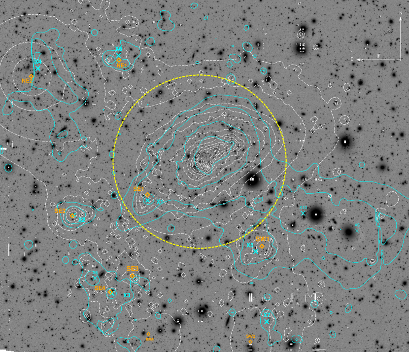
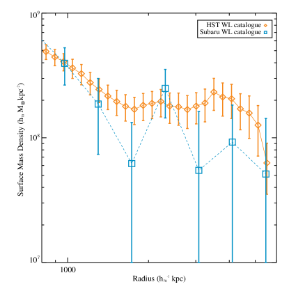
Our strong+weak lensing mass reconstruction of MACS J0717 reveals 9 substructures located between 1.6 and 4.9 Mpc in projection from the cluster core (: 109.39820; : 37.745778), which is itself composed of four merging clusters. Table 1 lists the substructures’ and the cluster core (Core) coordinates, masses, and detection significance. All substructures are also highlighted in Fig. 2 with orange diamonds. We note that the large-scale filament detected in Jauzac et al. (2012) is not illustrated clearly in Fig. 2. The structure is detected with 3 significance, a similar level as in Jauzac et al. (2012). However, we chose to draw contours that highlight the substructure detections, rather than the lower-density filament. Moreover, as a test of consistency between the Subaru and the HST weak-lensing analysis we compare the density profiles obtained in this region as shown in Fig. 1. Both profiles show a good agreement, with the Subaru one having larger error bars due to a much lower density of background galaxies.
The Core of MACS J0717 has been extensively studied due to its rich dynamical status, and therefore its lensing power. Its four main components are not the subject of this analysis, and are therefore all imbedded in the Core component (see Sect. 4.1). To test the reliability of our mass measurements, we first compare our mass values with published strong-lensing estimates from Limousin et al. (2016), Diego et al. (2015) and Kawamata et al. (2016). For their core model, Limousin et al. (2016) measure a total mass of , which is in excellent agreement with our measurement, . Diego et al. (2015) used a free-form method to build the strong-lensing mass model of MACS J0717 (WSLAP+, Diego et al., 2005, 2007; Ponente & Diego, 2011; Lam et al., 2014; Sendra et al., 2014), and measured a mass of (priv. comm.), which is in excellent agreement with our mass estimate within the same aperture, . Kawamata et al. (2016) used the parametric glafic algorithm (Oguri, 2010) and measured a total mass (priv. comm.). While their estimate is slightly higher than ours, it is of the same order.
We now discuss the several substructures detected on our strong- and weak-lensing mass map. SE1 and SE2 were previously detected in Jauzac et al. (2012), and as described in Sect. 6.2 both have an X-ray counterpart. They are also the most massive substructures found in MACS J0717 outskirts. The SE5, NE2 and SW2 substructures are all at the edge of the mass map. It is therefore difficult to disentangle between real substructures and artifacts from the mass modeling technique. Nevertheless, if they are real, the mass estimates should be taken with care. NE2 is discussed in more detail in Sect. 6.2. Finally, SE1, SE2, SE3, SE4 (and possibly SE5) are all embedded in the large-scale filament identified in Jauzac et al. (2012). Moreover, all the detected substructures show an optical counterpart, and appear to be at the redshift of the cluster when identifying their galaxy counterparts using photometric and spectroscopic redshifts from Ma et al. (2008). NE1, NE2 and SE2 are all three detected by Durret et al. (2016). This double identification confirms all three are at the cluster’s redshift, as Durret et al. (2016) detected them as overdensities of red-sequence galaxies.
| R.A. (deg) | Dec. (deg) | |||||
|---|---|---|---|---|---|---|
| Core | 109.3982 | 37.745778 | 130 | – | ||
| SW1 | 109.3087625 | 37.6497725 | 5 | 2.8 | ||
| SW2∗ | 109.3252847 | 37.54148293 | 0.51 | 3 | 4.9 | |
| SE1 | 109.4729667 | 37.70826611 | 10 | 1.6 | ||
| SE2 | 109.58105 | 37.68432278 | 8 | 3.6 | ||
| SE3 | 109.49475 | 37.61619444 | 5 | 3.5 | ||
| SE4 | 109.5261625 | 37.59775361 | 4 | 4.1 | ||
| SE5∗ | 109.4714417 | 37.5501475 | 3 | 4.7 | ||
| NE1 | 109.5142708 | 37.86093833 | 3 | 3.4 | ||
| NE2∗ | 109.6404125 | 37.84233667 | 3 | 4.9 |
| ID | R.A. (deg) | Dec. (deg) | kT [keV] | [ erg s-1] | |||
| X1 | 109.47288 | 37.701895 | SE1 | 0.04 | |||
| X2 | 109.57894 | 37.685011 | SE2 | 0.03 | |||
| X3 | 109.52414 | 37.596199 | SE4 | 0.03 | |||
| X4 | 109.63088 | 37.851494 | NE2 | 0.03 | |||
| X5 | 109.31781 | 37.643859 | SW1 | 0.01 | |||
| X6 | 109.51502 | 37.866279 | NE1 | 0.04 | |||
| X7 | 109.30196 | 37.564191 | SW2 | 0.02 | |||
| X8∗ | 109.54821 | 37.61343 | – | – | – | – | – |
| X9∗∗ | 109.17231 | 37.667292 | – | – | – | – | – |
| X10∗∗∗ | 109.24965 | 37.687168 | – | – | – | – | – |
6.2 X-ray & lensing properties of substructures
As already noted, MACS J0717’s core has been extensively studied in previous work (Ma et al., 2008; Mroczkowski et al., 2012; Adam et al., 2017b, a; van Weeren et al., 2017), and we thus refer the reader to these papers for a detailed analysis of the ongoing central merger. Here we focus on the distribution of substructures in the surroundings of MACS J0717.
Among the 9 substructures detected in the lensing map and listed in Table 1, two do not show a clear X-ray counterpart, SE3 and SE5. SE1 and SE2 are both detected in the X-ray, X1 and X2 respectively in Table 2. Those massive X-ray groups were already known and highlighted in Jauzac et al. (2012). The alignment between X-ray and lensing peaks is almost perfect, leading to the conclusion that these two substructures are virialized, or falling in along the line of sight. SE3 is close to X3, a complex extended X-ray substructure. While its X-ray peak aligns really well with SE4, it is not clear that one of its components, North West of X3, could not be associated with SE3. Indeed, this region of extended emission is apparently made of at least two and possibly three individual extended X-ray structures, as is shown by the cyan contours in Fig. 2. Moreover, this region is located at the edge of both the XMM-Newton and Subaru fields, thus uncertainties in the position of the substructures are large. For these reasons, the association of SE3 with X3 is likely.
NE1 is associated with X6, and both peaks are well aligned. NE2 shows a bright X-ray counterpart, X4. While in Sect. 6.1 we warned the reader that NE2 is located at the edge of the grid, the fact that in the X-ray a similar structure is detected makes us confident in that detection. However its lensing-mass estimate is biased by its proximity to the edge of the grid, and should thus be taken with care. SW1 is almost aligned with X5. This structure exhibits a flat and elongated X-ray morphology, which could indicate a previous interaction with the main halo. However, we caution that several X-ray bright foreground substructures (labelled as X9 and X10 in Fig. 2) are detected close to SW1 and may partly overlap with the X-ray emission associated with SW1/X5. Concerning SW2 and its X-ray counterpart, X7, both are located at the edge of the lensing-grid and at the limit of the XMM-Newton imaging, similar to NE2 and X5. While NE2 appears quite massive both in the lensing and X-ray maps, SW2 is the least massive substructure in our sample. It is therefore particularly difficult to disentangle between a grid artifact/edge of XMM-Newton field of view and a real detection. Concerning SE5, as we explain in Sect. 6.1, it is located at the edge of the constrained region, therefore it could reasonably be a grid artifact, and it is also located at the edge of the XMM-Newton field of view. Therefore we do not conclude on the existence of SE5. In comparison with NE2, which is clearly detected in both the lensing map and the X-ray map even if at the edge of the fields, SE5 is less massive.
| Core | 4.03 |
|---|---|
| SW1 | 1.90 |
| SE1 | 2.01 |
| SE2 | 2.07 |
| SE3 | 1.68 |
| SE4 | 1.16 |
| NE1 | 1.05 |
| NE2∗ | 2.02 |
In Table 2 we give the coordinates, the temperature, , the X-ray luminosity and the gas mass within an aperture of 250 kpc, and respectively, and for the X-ray remnant cores that have a correspondence with the lensing detections, their lensing ID, , as well as their gas fraction, . We note that X8, X9 and X10 do not have any lensing counterparts. To identify these substructures, we used the NED catalogue and found a corresponding object for each of them. X8 is associated with a bright spiral galaxy, 2MASSX J07180932+3737031, which is a GALEX source for which we could not get any redshift. X9 is a well-known submillimetre galaxy (SMG) at , 2MASSX J 07164427+3739556. Finally X10 does not have any match in the NED catalogue, however we suppose it is a foreground object as there is a bright galaxy at its position. Its proximity to X9 can lead to the assumption that it can be another foreground structure at a similar redshift as 2MASSX J07164427+3739556.
The gas fraction within a radius of R kpc for all substructures with a lensing counterpart varies between 1% and 4%. These relatively low gas fractions can be explained by two effects. First, each of these substructures are relatively low-mass/low-temperature groups within which we do not expect the total gas fraction to exceed 10% (see Fig. 20 in Vikhlinin et al. 2006 and Fig. 4 in Eckert et al. 2016b). Second, the gas and lensing masses are measured in an aperture smaller than the virial radius of the structures, meaning that we could be missing some of the gas content and therefore we tend to underestimate the total gas fraction.
As a consistency check, we also look at the mass-temperature relation of these groups, and compare it with the Lieu et al. (2016) – relation, expressed as:
| (4) |
with and , parameters derived from the XXL+COSMOS+CCCP sample. The masses are estimated by fitting a NFW profile (Navarro et al., 1997) to the integrated mass profiles we obtain for each of the substructures (see Table 3). Such an estimate should be considered as an upper limit, as it will tend to overestimate the mass while converting 2D projected masses into 3D masses. Moreover, due to the fact that substructures cannot be isolated from each other, the mass of one may contribute to the integrated mass profile of another one. However, while our statistics is limited, we compare our results with the – relation measured by Lieu et al. (2016). One of the group falls right on the Lieu et al. (2016) relation, and the other lie above the relation by up to a factor of 2. This suggests that the are overestimated.
| ID | |||
|---|---|---|---|
| Cluster 1 - SH 1 | 0.00 | 0.00 | 0.00 |
| Cluster 1 - SH 2 | 3.88 | 0.86 | 0.51 |
| Cluster 1 - SH 3 | 1.61 | 0.53 | 0.53 |
| Cluster 1 - SH 4 | 3.23 | 0.64 | 1.02 |
| Cluster 1 - SH 5 | 2.68 | 1.44 | 0.79 |
| Cluster 1 - SH 6 | 3.80 | 0.92 | 0.32 |
| Cluster 1 - SH 7 | 0.81 | 0.93 | 0.60 |
| Cluster 1 - SH 8 | 3.02 | 1.50 | 0.88 |
| Cluster 2 - SH 1 | 0.00 | 0.00 | 0.00 |
| Cluster 2 - SH 2 | 0.85 | 0.86 | 0.72 |
| Cluster 2 - SH 3 | 4.30 | 1.36 | 1.02 |
| Cluster 2 - SH 4 | 1.17 | 0.46 | 0.95 |
| Cluster 2 - SH 5 | 0.89 | 0.86 | 0.60 |
| Cluster 2 - SH 6 | 3.15 | 0.94 | 0.63 |
| Cluster 2 - SH 7 | 0.32 | 0.49 | 0.45 |
7 Comparison of simulations and observations
Our goal is to observationally probe cluster evolution. MACS J0717 is a rare object due to its mass and dynamical state at . It is with such objects that we can test the limits of the cosmological paradigm. In two previous papers (Jauzac et al., 2016; Schwinn et al., 2017), we looked at a similar cluster, Abell 2744, at a lower redshift, . Abell 2744 has a similarly complex substructure distribution, including 7 substructures within 2 Mpc of the cluster centre (plus one background substructure identified spectroscopically, a superposition along the line of sight). Additionally 3 large-scale filaments extending out to 7 Mpc that were detected by Eckert et al. (2015). Our present analysis also finds 7 substructures around MACS J0717 (discarding the 2 being at the edge of the mass map and XMM-Newton field of view), but these are farther from the cluster centre: only one (SE1) is within 2 Mpc of the core, and the rest extend to 5 Mpc.
| ID | |||
|---|---|---|---|
| Cluster 1 - SH 1 | 12.67 | 30.66 | 32.70 |
| Cluster 1 - SH 2 | 1.62 | 0.36 | 0.17 |
| Cluster 1 - SH 3 | 0.41 | 0.10 | 0.17 |
| Cluster 1 - SH 4 | 1.24 | 0.25 | 0.22 |
| Cluster 1 - SH 5 | 0.92 | 0.36 | 0.30 |
| Cluster 1 - SH 6 | 0.19 | 0.07 | 0.02 |
| Cluster 1 - SH 7 | 0.86 | 0.19 | 0.10 |
| Cluster 1 - SH 8 | 0.89 | 0.38 | 0.23 |
| Cluster 2 - SH 1 | 14.60 | 27.30 | 29.57 |
| Cluster 2 - SH 2 | 0.10 | 0.04 | 0.03 |
| Cluster 2 - SH 3 | 3.07 | 1.46 | 0.61 |
| Cluster 2 - SH 4 | 1.22 | 0.34 | 0.40 |
| Cluster 2 - SH 5 | 0.12 | 0.06 | 0.05 |
| Cluster 2 - SH 6 | 0.01 | 0.002 | 0.01 |
| Cluster 2 - SH 7 | 0.05 | 0.04 | 0.03 |
Given the redshift, mass and distribution of its substructure, we hypothesize that MACS J0717 is the progenitor of a structure that will look very similar to Abell 2744 by redshift . To test this hypothesis, we compare our observations of these two clusters with clusters in the numerical simulations MXXL (Angulo et al., 2012) and Hydrangea/C-EAGLE (Bahé et al., 2017; Barnes et al., 2017b). We shall first check whether clusters as rich in substructure as MACS J0717 and Abell 2744 even exist in a CDM model. Then we shall consider the mass growth rate and substructure infall rate of similar simulated clusters, in a way that is impossible in real systems that can be observed only in a snapshot at a single redshift.
7.1 Identification of simulated analogues
7.1.1 Comparison with MXXL
We use the two halos with similar properties to Abell 2744 presented in Sect. 3.1 to investigate the infall of substructures into halos. The reason for looking for Abell 2744 analogues rather than MACS J0717’s is simply motivated by the lack of particle data output around with MXXL. We only have particle data at , thus closer to Abell 2744’s redshift. We therefore look for Abell 2744-like clusters (substructures close to the cluster’s main halo) and trace them back in time using subhalo catalogues up to a redshift closer to MACS J0717’s. Cluster 1 has a mass of at and the second cluster (Cluster 2) has a mass of , both within the 3-range of Abell 2744’s mass. For both of these halos, we create mass maps at by projecting all particles over a distance of onto a map. Substructures within these halos are then identified as over-densities within these maps and we check wether their mass within an aperture of 150 kpc lies within the interval of the masses obtained for Abell 2744 substructures.
Nonetheless, as mentioned in Sect. 3.1, MXXL particle data are only available at a very small number of redshifts. If we want to analyse the evolution of the identified subhalos up to to compare with MACS J0717, we are dependent on the subfind datasets of all other snapshots for which the particle data are not available. We thus identify the subfind-subhalos closest to the position of each subhalo identified in our projected mass map. We then use the merger trees available for each subfind-subhalo in MXXL to trace the evolution of each subhalo back in time, at (particle data), and finally .
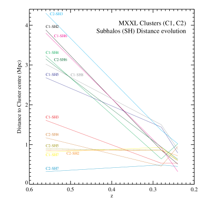
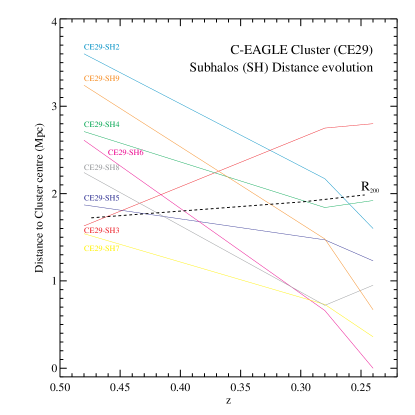
Table 4 lists the change in radial distances and Table 5 lists subfind-masses of the Abell 2744-like substructures in both MXXL clusters. We list distances and masses at , corresponding to the snapshot closest to MACS J0717’s redshift, at , the snapshot closest to Abell 2744’s redshift, and then , the snapshot where particle data are available. For each subhalo, the radial 2D-distance projected along the line of sight and the subfind-masses are given. The analysis of these two MXXL clusters shows that subhalos move by a distance of 2-3 Mpc between the redshifts of MACS J0717 and Abell 2744. While the subhalos already close to the virial radius do not move much, the rest of the substructures get closer to the main halo centre by 2-3 Mpc. Figure 3 shows the infalling distance of subhalos as a function of redshift for Cluster 1 and Cluster 2 .
The substructures that fall in from the furthest distances correspond mostly to the most massive substructures at redshift . During their infall their subfind-masses decrease quite dramatically, in three cases by over 70%. However, it is important to be very careful when comparing subfind-masses to aperture masses from gravitational lensing analysis. One reason for this discrepancy is that subfind only assigns particles to a subhalo that are gravitationally bound to it. While this is a reasonable thing to do from a theoretical point of view, the substructures identified by this method are not easily comparable to those identified in gravitational lensing mass maps. In the latter, tidally stripped material and also the background halo contribute significantly to the subhalo masses (Mao et al., 2017). The degree of tidal stripping plays an important role here, which can be seen by the fact that the mass of three subhalos drops by over 70% (see Table 5). For a direct comparison of masses of simulated subhalos to masses of observed subhalos, it is much more reliable to obtain the subhalo 2D-projected masses from the simulation particle data if available.
Finally we looked at the mass gain of the main halos of Cluster 1 and Cluster 2 considering the evolution of between and . We measure a mass growth of and . If we consider the mass growth between and , we obtain and .
| ID | |||||
|---|---|---|---|---|---|
| CE29 - SH 1 | 20.1 | 59.8 | 0 | 0 | 0.03 |
| CE29 - SH 2 | 9.16 | 48.9 | 3.60 | 440 | 0.05 |
| CE29 - SH 3 | 1.64 | 0.9 | 1.63 | -1100 | 0.01 |
| CE29 - SH 4 | 1.09 | 2.7 | 2.71 | 290 | 0.03 |
| CE29 - SH 5 | 1.02 | 0.4 | 1.87 | 300 | 0.004 |
| CE29 - SH 6 | 1.47 | 6.4 | 2.61 | 1070 | 0.04 |
| CE29 - SH 7 | 1.04 | 0.8 | 1.54 | 1290 | 0.01 |
| CE29 - SH 8 | 1.05 | 0.2 | 2.24 | 1280 | 0.002 |
| CE29 - SH 9 | 1.01 | 0.004 | 3.24 | 950 |
7.1.2 Comparison with Hydrangea/C-EAGLE
For the purpose of our comparison, we use the most massive halo (CE-29) present in the simulation. At this cluster has a radius , a mass , a soft X-ray luminosity of , a spectroscopic temperature and is the host of galaxies with a stellar mass (Bahé et al., 2017; Barnes et al., 2017b).
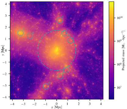
We analyse the snapshot of the simulation closest to the redshift of MACS J0717 at . We extract a cube of side-length centered around the minimum of the potential of the halo. To construct a mass map, we project all the particles along the z-axis of the simulation volume and bin them using a regular grid with cells of side-length . The result of this procedure is shown in Fig. 4 with the dashed circle corresponding to the projected spherical over-density radius . Compared to actual weak-lensing data, this projected mass map is an idealised mass map where any foreground and background structures perturbing the signal have been removed.
| ID | |||
|---|---|---|---|
| CE29 - SH 1 | 9.15 | 9.76 | 10.70 |
| CE29 - SH 2 | 2.07 | 1.89 | 1.57 |
| CE29 - SH 3 | 1.68 | 1.37 | 1.32 |
| CE29 - SH 4 | 6.46 | 5.43 | 4.74 |
| CE29 - SH 5 | 5.55 | 4.56 | 4.55 |
| CE29 - SH 6 | 1.48 | 1.46 | merged |
| CE29 - SH 7 | 4.23 | 2.82 | 1.63 |
| CE29 - SH 8 | 3.13 | 2.37 | 2.76 |
| CE29 - SH 9 | 3.13 | 3.22 | 1.19 |
| ID | |||
|---|---|---|---|
| CE29 - SH 1 | 0.00 | 0.00 | 0.00 |
| CE29 - SH 2 | 3.60 | 2.17 | 1.60 |
| CE29 - SH 3 | 1.63 | 2.75 | 2.80 |
| CE29 - SH 4 | 2.71 | 1.84 | 1.92 |
| CE29 - SH 5 | 1.87 | 1.47 | 1.23 |
| CE29 - SH 6 | 2.61 | 0.66 | 0.00 |
| CE29 - SH 7 | 1.54 | 0.73 | 0.36 |
| CE29 - SH 8 | 2.24 | 0.72 | 0.95 |
| CE29 - SH 9 | 3.24 | 1.48 | 0.67 |
We then construct a catalogue of weak-lensing detected objects. We start by selecting all the haloes and sub-haloes identified by the Subfind algorithm with a mass above and compute the total projected mass in a circular aperture around their centre of potential. In a second step we discard all such sub-structures with a projected mass under . This is slightly lower than the smallest object detected around MACS J0717 but is designed to allow for a systematical overestimation of the masses in the weak-lensing data. As pointed out by Schwinn et al. (2017) and more quantitatively by Mao et al. (2017), Subfind masses two orders of magnitude lower than a given aperture mass can be boosted by projection effects to reach the mass threshold. As we are aiming for a projected aperture mass of , our first selection of sub-haloes with a subfind mass above is justified. This procedure, however, does not guarantee that the structures analysed in this way would be detectable. An additional step to identify detectable overdensities is required. We hence iterate over all the substructures from the most massive to the least massive and eliminate the ones that overlap with a more massive object or that are within of the centre of the halo. This step is necessary as there is no way observationally to distinguish structures that overlap in projection. At the end of this procedure, we are left with 8 sub-haloes shown as small cyan circles on Fig. 4 with their masse, projected distance to the centre and velocity towards the centre of the cluster given in the first three columns of Table 6. The mass and distance range is similar to what we observe in MACS J0717. We also analysed the companion simulation without baryon physics and found projected masses in excellent agreement. This demonstrates that baryonic processes have little effects on these weak lensing mass measurements.
From the total masses of the halo (), we can estimate a mass growth rate between and of . Moreover, between and we measure a mass growth rate . We note that CE-29 is undergoing a major merger at , which is responsible for such a high mass growth.
In Table 7 and Table 8 we show the evolution of the projected distance of the subhalos and their subfind masses between and . This is the closest we can get with available particle data to the respective redshifts of MACS J0717 and Abell 2744. As one can see in Fig. 5, they all have entered the virial radius region, except for CE29 - SH3 which is a back-splash sub-halo that will return towards the centre of the cluster at a later time. The average projected distance travelled to the main halo between and is in the range of 1-2 Mpc as can be seen in Fig. 5.
As discussed above, the subfind masses cannot be related in a straightforward way to the projected mass within that can be observationally measured. Mao et al. (2017) showed that sub-halos embedded in a large halo can see their ratio of projected mass over Subfind mass reach values as large as . Similar boosts can also be seen in the substructures detected outside the virial radius but part of the larger over-density around the cluster. This can be seen by comparing the masses reported in Table 6 and Table 7.
7.2 Properties of a high redshift super-cluster
7.2.1 Infall of Substructures
MACSJ 0717 substructures seem to be distributed along three preferred directions: South-East, North-East and South-West, with neither lensing nor X-ray substructures detected in the North-West region as can be seen in Fig. 2. In the context of hierarchical structure formation scenarios, halos are expected to be located at the intersection of three large-scale filaments (Bond et al., 1996), as was observed around Abell 2744 (Eckert et al., 2015). Nevertheless, all the dark matter substructures along with their X-ray counterparts, apart from the Core and SE1, appear to be located outside the virial radius of MACS J0717 (yellow circle on Fig. 2). However, Lau et al. (2015) show that up to 3R200 (7 Mpc), these substructures are already decoupled from the Hubble flow and therefore infalling into the cluster. Therefore, looking at both the dark and luminous mass distribution of MACS J0717, it is reasonable to assume that these detected substructures are falling into the cluster’s main halo, and are doing so along three preferred directions, one of them at the location of which a dark matter large-scale filament was detected by Jauzac et al. (2012). However, only higher quality X-ray and weak-lensing data will enable us to confirm this assumption.
To start our investigation, we first estimate the distance that substructures like the ones observed here, would travel within the redshift interval between MACS J0717 and Abell 2744. For this we calculate the interval in look-back time, , for both cluster redshifts using the following expression:
| (5) |
where,
| (6) |
Applying equation 5 to the redshifts of Abell 2744 and MACS J0717 we obtain yr, and yr. That gives us a look back time yr. If we make the hypothesis that the observed substructures in MACS J0717 are typical groups which have an infall velocity of km.s-1 (Lau et al., 2015), thus we estimate that between and , the typical infall distance of substructures should be 2 Mpc. This value is a lower limit estimate due to both projection effects and the fact that once substructures have entered the virial radius region, their infall velocity will increase as they are getting closer to the centre of the main halo.
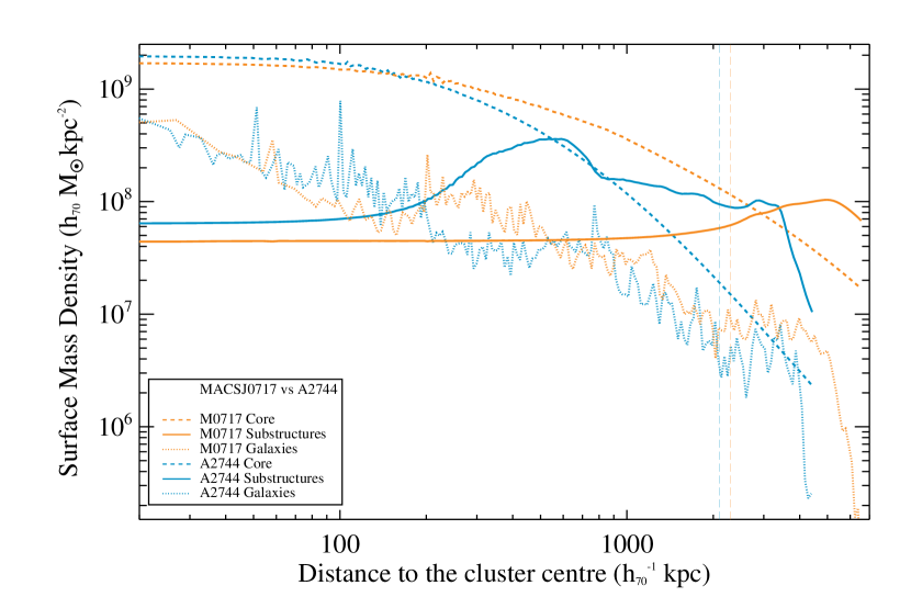
Figure 6 shows the density profiles of both MACS J0717 (orange) and Abell 2744 (cyan) as a function of the distance to the cluster centre for each of their components: the core of the cluster (dashed line), the substructure contribution (plain line) and the contribution from galaxies (dotted lines). We also highlight their respective as vertical lines ( Mpc; Mpc). From the core profiles, one can clearly see the different evolution stages between the two clusters: MACS J0717 has a slightly less dense but more extended core than Abell 2744, a typical signature of the change of the mass-concentration relation with redshift and mass. With time, substructures will infall and merge, the core density will increase and become more ‘peaky’ while leaving the outskirts of the cluster slightly under-dense as can be seen in Abell 2744. While substructures often refer to galaxies, we here refer to group to cluster-scale halos (). The substructure profiles in Fig. 6 clearly show the different evolutionary stages of the two clusters: the density of the substructure distribution peaks around 5-6 Mpc in MACSJ 0717, and peaks at 1 Mpc followed by a plateau up to 4.5 Mpc (limit of the field of view) in Abell 2744. This change of slope in Abell 2744 substructure’s density profile is due to the presence of the large-scale filaments detected by Eckert et al. (2015). As a matter of consistency, we show all the clusters’ components in Fig. 6. While the evolution stage of the object plays a key role in the shape of the density profiles of both the core and the substructure profiles, one can see that the galaxy density profiles for both clusters are similar and follow a similar slope. Applying our above infall distance estimate between and to MACS J0717 would mean that all the substructures would reach the virial radius by .
However, this analytic approach is limited. That is why we turn to numerical simulations such as MXXL (Angulo et al., 2012) and Hydrangea/C-EAGLE (Bahé et al., 2017; Barnes et al., 2017b) in order to trace these ‘independent’ substructures (i.e. at ) between and and measure their average infall distance. In Abell 2744, all the substructures are detected within less than 2 Mpc from the core (excluding the filamentary structures outside ). Therefore all substructures are assumed to be virialized within the main halo, which is not the case for MACS J0717. As explained at the beginning of this Section, one motivation behind this analysis is to see if the assumption that MACS J0717 could be a progenitor of an Abell 2744-like cluster is realistic in terms of substructure infall and thus distribution. According to the calculation made earlier, it appears to be sensible (considering 2 Mpc as a lower limit of infall distance between the redshift of the two clusters) to postulate that the actual substructures visible in MACS J0717 outskirts would have reached by redshift , and is in good agreement with both MXXL and Hydrangea/C-EAGLE.
7.2.2 Mass growth rate
We now estimate the mass growth of MACS J0717. In order to estimate the growth due to substructure infall, we fit a NFW profile to all the secured substructures (see Sect. 6.2 and Table 3), i.e. excluding SE5 and SW2 from our calculations as well as SE1 which is already in the main halo ( Mpc). We can thus estimate a total mass of substructures 0.9810. Applying a similar fit to the Core component, we obtain a mass 4.0310. Therefore, considering that all these substructures will be merging with the cluster main halo within at , we can estimate that the mass growth of MACS J0717 due to massive substructures will be of a factor of 1.25 (over yr).
When we compare the mass growth of MACS J0717 due to these substructures only we can see a good agreement with the mass growth estimated from Hydrangea/C-EAGLE () and slightly lower than MXXL measurements ( and ). Nevertheless, a few caveats have to be emphasized: (1) the MACS J0717 calculation relies on our conversion of aperture projected masses into , and thus may lead to an overestimation of the mass growth rate, and (2) the growth rate relies on projected masses, however as shown by Mao et al. (2017) such masses can be overestimated by up to 2 orders of magnitude. Our relative agreement with numerical simulations could lead to the conclusion that the mass growth rate of these ‘cosmic beasts’ is not dominated by the smooth accretion of surrounding material (low mass substructures, i.e. not groups nor clusters), but rather by events of massive substructure infall. However, the true masses of the simulated substructures are given in Table 5 and Table 7. We note that the difference between those and their projected estimates can reach several order of magnitudes which is in agreement with Mao et al. (2017). That is suggesting that the majority of the mass growth measured for the simulated clusters is due to smooth accretion of low mass substructures rather than infall of massive substructures.
MACS J0717’s substructure distribution (up to Mpc) and total mass leads us to the conclusion that we are observing a super-cluster (Einasto et al., 2001; Einasto et al., 2007; Chon et al., 2013), similar to what is observed in Pompei et al. (2016) at . If by MACS J0717 has virialized, it will form an extremely massive cluster of considering the average mass growth rate of 2.9 measured from both MXXL and C-EAGLE clusters -. The clusters considered with MXXL and Hydrangea/C-EAGLE are the most massive objects visible in the simulations, and are all three undergoing extreme merger events between , making the average growth rate relatively large. However, considering the complexity of MACS J0717, we could expect it to undergo such an extreme dynamical history.
7.2.3 Gas fraction in substructures
Finally, we took advantage of the Hydrangea/C-EAGLE simulation that includes baryons in order to compare our measured gas fractions with the ones of the CE-29 substructures. The gas mass, , of each CE-29 substructures measured within an aperture of 250 kpc and the gas fraction, , are reported in Table 6. We here consider the hot gas mass in order to compare our results with what is measured in MACS J0717.
We measure relatively low gas fractions, between 1% and 5%. This is in excellent agreement with MACS J0717 gas fractions as reported in Table 2. It confirms our initial hypothesis of an underestimated gas fraction due to a small aperture (not extending up to ), as well as the reliability of the baryonic physics in the Hydrangea/C-EAGLE suite of simulations.
8 Conclusions
The masses and distribution of substructures in the outskirts of massive galaxy clusters provide an observational test of the CDM structure formation paradigm and at the same time present an opportunity to quantify the importance of major mergers in the buildup of these extreme objects. We have performed a combined strong-, weak-lensing, and X-ray analysis of observations from the HST, Subaru, Chandra, and XMM-Newton telescopes. We detected substructures in the outskirts of one of the most massive galaxy clusters in the observable Universe, MACS J0717 at , using the hybrid version of the lenstool software (Jullo et al., 2007; Jullo et al., 2010; Jauzac et al., 2012, 2015a). To interpret our findings, we have compared our observational results to our previous analysis of the massive cluster Abell 2744 at (Jauzac et al., 2016) and two different cosmological simulations, MXXL (Angulo et al., 2012) and Hydrangea/C-EAGLE (Bahé et al., 2017; Barnes et al., 2017b).
Observational results
Our key observational results may be summarized as follows:
-
1.
We detect 9 group-scale substructures with masses ranging between located between 1.6 and 4.9 Mpc from the cluster centre.
-
2.
The X-ray analysis of the XMM-Newton and Chandra data reveals 10 substructures.
-
3.
The combination with X-ray data allowed us to secure 7 of the lensing detections.
-
4.
The X-ray data show 3 substructures not detected in the lensing mass map (X8, X9 and X10) that we identified as being possible foreground objects in the NED catalogue.
- 5.
-
6.
We look at the -T relation for these groups and compare our results with Lieu et al. (2016). This confirms the overestimation of our .
Comparison with MXXL Hydrangea/C-EAGLE
Our key results from the comparison with numerical simulations can be summarized as follows:
-
1.
Clusters as rich in substructure as MACS J0717 and Abell 2744 are common in cosmological simulations, if the simulation data are analysed in a way compatible to the observations.
-
2.
Projected mass maps of the two most massive clusters in the MXXL dark-matter only simulation, and the most massive cluster in the hydrodynamical Hydrangea/C-EAGLE simulation (CE-29) all reveal a similar number of massive substructures as what is observed. The substructures in the latter also have hot gas fractions that are in excellent agreement with MACS J0717 (Figs. 3, 4, and 5).
-
3.
From the total halo mass of the two MXXL clusters, we can estimate a mass growth rate of a factor of 3.7 and 1.9 for Cluster 1 and Cluster 2 respectively between and , and of a factor of 4.0 and 2.5 between and .
-
4.
For the first time we confronted theory and observations of gas fractions in massive galaxy clusters using state-of-the-art hydrodynamical simulations. We measured the gas fraction within an aperture of 250 kpc for each of CE-29 substructures, between 1% and 5%, which is in excellent agreement with what is observed in MACS J0717. From the evolution of the total halo mass in the Hydrangea/C-EAGLE cluster, , we estimated a mass growth of a factor of 1.2 between and .
Mass growth of MACS J0717
The substructure distribution in MACS J0717 is quite similar to what we observed in Abell 2744: seven substructures at the cluster redshift detected in both cases, with relatively lower masses in the case of MACS J0717 and more distant to the cluster centre. Such behavior is expected while looking at the redshift difference between the two clusters, one being at a more advanced evolution stage than the other. Therefore we ask ourselves the question of wether MACS J0717-like clusters coud be the progenitors of Abell 2744-like clusters:
-
1.
A comparison between MACS J0717 and Abell 2744 suggests that the substructures we have identified in the former will move in towards the cluster centre by 2–3 Mpc between and . This agrees with both analytic expectations and the radial motion of substructures in the simulations, and suggests that MACS J0717 will, over time, evolve into a system similar to Abell 2744 in terms of substructure distribution.
-
2.
Compared to Abell 2744, the core of MACS J0717 shows a more extended mass profile of its core and substructure components, while the mass profiles from their individual member galaxies agree well. We interpret this as evidence for a less evolved state of MACS J0717, as might be expected from its higher redshift and mass (Fig. 6).
-
3.
From the lensing masses and expected infall velocity of the MACS J0717 substructures, we estimate a mass growth due to the accretion of massive substructures of a factor of 1.25 between and , i.e. over a period of 2.1 Gyr. This is close to the total growth of the simulated cluster CE-29 over a similar redshift interval (1.20), but lower than the growth of either of the two MXXL clusters (3.7 and 1.9, respectively). Taking into account that our lensing-derived substructure masses are likely overestimated, this implies that the growth of ‘cosmic beast’ is dominated by the smooth accretion of surrounding material (low-mass substructures) rather than regular massive substructure infall events.
A super-cluster at
MACS J0717 is a super-cluster at (Einasto et al., 2001; Einasto et al., 2007; Chon et al., 2013; Pompei et al., 2016). Extrapolating its mass growth with expectations from simulations, it has likely evolved into an extremely massive cluster of by the present day. We have shown that such massive systems are commonly surrounded by a large number of group-scale substructures, in agreement with recent observations at lower redshift (Haines et al., 2017) and cosmological simulations in a CDM cosmology. Rather than constituting a challenge to our understanding of structure formation, our study has demonstrated that such objects offer a unique opportunity to directly observe the assembly of massive galaxy clusters. In the near future, we can hope to exploit this further by analyzing the substructure content of other massive clusters, and extending it to proto-clusters at higher redshift. Combined with cosmological simulations, such observations will enable a detailed probe of the assembly of ‘cosmic beasts’, the most massive bound structures in the Universe.
Acknowledgements
We thank the anonymous referee for their comments which helped improve our paper.
This work would not have been possible without Lydia Heck and Peter Draper’s computing expertise. We thank John Helly for his help with merger trees, and R. Kawamata and J. M. Diego for sharing their integrated mass profiles.
This work was supported by the Science and Technology Facilities Council (grant numbers ST/L00075X/1, ST/P000451/1) and used the DiRAC Data Centric system at Durham University, operated by the Institute for Computational Cosmology on behalf of the STFC DiRAC HPC Facility (www.dirac.ac.uk). This equipment was funded by BIS National E-infrastructure capital grant ST/K00042X/1, STFC capital grant ST/H008519/1, and STFC DiRAC Operations grant ST/K003267/1 and Durham University. DiRAC is part of the National E-Infrastructure. The Hydrangea/C-EAGLE simulations were in part performed on the German federal maximum performance computer “HazelHen” at the maximum performance computing centre Stuttgart (HLRS), under project GCS-HYDA / ID 44067 financed through the large-scale project “Hydrangea” of the Gauss Center for Supercomputing. Further simulations were performed at the Max Planck Computing and Data Facility in Garching, Germany. This project has received funding from the European Union’s Horizon 2020 research and innovation programme under the Marie Sklodowska-Curie grant agreement No 747645. MJ, EJ and ML acknowledge the support of the Centre National d’Études Spatiales (CNES). MJ, ML, and EJ acknowledge the Mésocentre d’Aix-Marseille Université (project number: 14b030). This study also benefited from the facilities offered by CeSAM (Centre de donnéeS Astrophysique de Marseille (http://lam.oamp.fr/cesam/). DE acknowledges the funding support from the Swiss National Science Foundation (SNSF). RM is supported by the Royal Society. CDV acknowledges financial support from the Spanish Ministry of Economy and Competitiveness (MINECO) through grants AYA2014-58308 and RYC-2015-1807. JPK and MJ acknowledge support from the ERC advanced grant LIDA. ML acknowledges the Centre National de la Recherche Scientifique (CNRS) for its support. MN acknowledges PRIN INAF 2014 1.05.01.94.02. PN acknowledges support from the National Science Foundation via the grant AST-1044455, AST-1044455, and a theory grant from the Space Telescope Science Institute HST-AR-12144.01-A. KU acknowledges support from the Ministry of Science and Technology of Taiwan through the grant MoST 106-2628-M-001-003-MY3.
Facilities: This paper uses data from Hubble Space Telescope programmes GO-09722, GO-11560, GO-12103, GO-13498.
References
- Acebron et al. (2017) Acebron A., Jullo E., Limousin M., Tilquin A., Giocoli C., Jauzac M., Mahler G., Richard J., 2017, MNRAS, 470, 1809
- Adam et al. (2017a) Adam R., et al., 2017a, preprint, (arXiv:1706.10230)
- Adam et al. (2017b) Adam R., et al., 2017b, A&A, 598, A115
- Angulo et al. (2012) Angulo R. E., Springel V., White S. D. M., Jenkins A., Baugh C. M., Frenk C. S., 2012, Monthly Notices of the Royal Astronomical Society, 426, 2046
- Aragón-Calvo et al. (2010) Aragón-Calvo M. A., van de Weygaert R., Jones B. J. T., 2010, MNRAS, 408, 2163
- Arnouts et al. (1999) Arnouts S., Cristiani S., Moscardini L., Matarrese S., Lucchin F., Fontana A., Giallongo E., 1999, MNRAS, 310, 540
- Bahé et al. (2017) Bahé Y. M., et al., 2017, MNRAS, 470, 4186
- Barnes et al. (2017a) Barnes D. J., Kay S. T., Henson M. A., McCarthy I. G., Schaye J., Jenkins A., 2017a, MNRAS, 465, 213
- Barnes et al. (2017b) Barnes D. J., et al., 2017b, MNRAS, 471, 1088
- Bertin & Arnouts (1996) Bertin E., Arnouts S., 1996, A&A, 117, 393
- Bond et al. (1996) Bond J. R., Kofman L., Pogosyan D., 1996, Nature, 380, 603
- Booth & Schaye (2009) Booth C. M., Schaye J., 2009, MNRAS, 398, 53
- Bradac et al. (2006) Bradac M., et al., 2006, ArXiv Astrophysics e-prints,
- Cen & Ostriker (1999) Cen R., Ostriker J. P., 1999, ApJ, 519, L109
- Chirivì et al. (2017) Chirivì G., Suyu S. H., Grillo C., Halkola A., Balestra I., Caminha G. B., Mercurio A., Rosati P., 2017, preprint, (arXiv:1706.07815)
- Chon et al. (2013) Chon G., Böhringer H., Nowak N., 2013, MNRAS, 429, 3272
- Clowe et al. (2004) Clowe D., Gonzalez A., Markevitch M., 2004, ApJ, 604, 596
- Clowe et al. (2006) Clowe D., Bradač M., Gonzalez A. H., Markevitch M., Randall S. W., Jones C., Zaritsky D., 2006, ApJ, 648, L109
- Crain et al. (2015) Crain R. A., et al., 2015, MNRAS, 450, 1937
- Dalla Vecchia & Schaye (2012) Dalla Vecchia C., Schaye J., 2012, MNRAS, 426, 140
- Davé et al. (2001) Davé R., et al., 2001, ApJ, 552, 473
- Davis et al. (1985) Davis M., Efstathiou G., Frenk C. S., White S. D. M., 1985, AJ, 292, 371
- De Grandi et al. (2016) De Grandi S., et al., 2016, A&A, 592, A154
- De Luca & Molendi (2004) De Luca A., Molendi S., 2004, A&A, 419, 837
- Diego et al. (2005) Diego J. M., Sandvik H. B., Protopapas P., Tegmark M., Benítez N., Broadhurst T., 2005, MNRAS, 362, 1247
- Diego et al. (2007) Diego J. M., Tegmark M., Protopapas P., Sandvik H. B., 2007, MNRAS, 375, 958
- Diego et al. (2015) Diego J. M., Broadhurst T., Zitrin A., Lam D., Lim J., Ford H. C., Zheng W., 2015, MNRAS, 451, 3920
- Dolag et al. (2009) Dolag K., Borgani S., Murante G., Springel V., 2009, MNRAS, 399, 497
- Durret et al. (2016) Durret F., et al., 2016, A&A, 588, A69
- Ebeling et al. (2001) Ebeling H., Edge A. C., Henry J. P., 2001, ApJ, 553, 668
- Ebeling et al. (2004) Ebeling H., Barrett E., Donovan D., 2004, ApJ, 609, L49
- Ebeling et al. (2007) Ebeling H., Barrett E., Donovan D., Ma C.-J., Edge A. C., van Speybroeck L., 2007, ApJ, 661, L33
- Ebeling et al. (2014) Ebeling H., Ma C.-J., Barrett E., 2014, ApJS, 211, 21
- Eckert et al. (2014) Eckert D., et al., 2014, A&A, 570, A119
- Eckert et al. (2015) Eckert D., et al., 2015, Nature, 528, 105
- Eckert et al. (2016a) Eckert D., Jauzac M., Vazza F., Owers M., Kneib J.-P., Tchernin C., Intema H., Knowles K., 2016a, preprint, (arXiv:1603.02272)
- Eckert et al. (2016b) Eckert D., et al., 2016b, A&A, 592, A12
- Eckert et al. (2017) Eckert D., et al., 2017, preprint, (arXiv:1705.05844)
- Edge et al. (2003) Edge A. C., Ebeling H., Bremer M., Röttgering H., van Haarlem M. P., Rengelink R., Courtney N. J. D., 2003, MNRAS, 339, 913
- Einasto et al. (2001) Einasto M., Einasto J., Tago E., Müller V., Andernach H., 2001, AJ, 122, 2222
- Einasto et al. (2007) Einasto M., et al., 2007, A&A, 476, 697
- Elíasdóttir et al. (2007) Elíasdóttir Á., et al., 2007, preprint, 710 (arXiv:0710.5636)
- Fakhouri & Ma (2008) Fakhouri O., Ma C.-P., 2008, MNRAS, 386, 577
- Fang et al. (2002) Fang T., Marshall H. L., Lee J. C., Davis D. S., Canizares C. R., 2002, ApJ, 572, L127
- Fang et al. (2007) Fang T., Canizares C. R., Yao Y., 2007, ApJ, 670, 992
- Galeazzi et al. (2009) Galeazzi M., Gupta A., Ursino E., 2009, ApJ, 695, 1127
- Gao et al. (2012) Gao L., Navarro J. F., Frenk C. S., Jenkins A., Springel V., White S. D. M., 2012, MNRAS, 425, 2169
- Genel et al. (2010) Genel S., Bouché N., Naab T., Sternberg A., Genzel R., 2010, ApJ, 719, 229
- Gilmore & Natarajan (2009) Gilmore J., Natarajan P., 2009, MNRAS, 396, 354
- Haardt & Madau (2001) Haardt F., Madau P., 2001, in Neumann D. M., Tran J. T. V., eds, Clusters of Galaxies and the High Redshift Universe Observed in X-rays. (arXiv:astro-ph/0106018)
- Haines et al. (2017) Haines C. P., et al., 2017, preprint, (arXiv:1709.04945)
- Harvey et al. (2015) Harvey D., Massey R., Kitching T., Taylor A., Tittley E., 2015, Science, 347, 1462
- Hickox & Markevitch (2006) Hickox R. C., Markevitch M., 2006, ApJ, 645, 95
- Hoekstra et al. (2013) Hoekstra H., Bartelmann M., Dahle H., Israel H., Limousin M., Meneghetti M., 2013, Space Sci. Rev., 177, 75
- Hopkins (2013) Hopkins P. F., 2013, MNRAS, 428, 2840
- Ichinohe et al. (2015) Ichinohe Y., Werner N., Simionescu A., Allen S. W., Canning R. E. A., Ehlert S., Mernier F., Takahashi T., 2015, MNRAS, 448, 2971
- Ilbert et al. (2006) Ilbert O., et al., 2006, A&A, 457, 841
- Ilbert et al. (2009) Ilbert O., et al., 2009, ApJ, 690, 1236
- Jauzac et al. (2012) Jauzac M., et al., 2012, MNRAS, 426, 3369
- Jauzac et al. (2015a) Jauzac M., et al., 2015a, MNRAS, 446, 4132
- Jauzac et al. (2015b) Jauzac M., et al., 2015b, MNRAS, 452, 1437
- Jauzac et al. (2016) Jauzac M., et al., 2016, MNRAS, 463, 3876
- Jenkins (2010) Jenkins A., 2010, MNRAS, 403, 1859
- Johnson & Sharon (2016) Johnson T. L., Sharon K., 2016, ApJ, 832, 82
- Jullo & Kneib (2009) Jullo E., Kneib J., 2009, MNRAS, 395, 1319
- Jullo et al. (2007) Jullo E., Kneib J.-P., Limousin M., Elíasdóttir Á., Marshall P. J., Verdugo T., 2007, New Journal of Physics, 9, 447
- Jullo et al. (2010) Jullo E., Natarajan P., Kneib J.-P., D’Aloisio A., Limousin M., Richard J., Schimd C., 2010, Science, 329, 924
- Jullo et al. (2014) Jullo E., Pires S., Jauzac M., Kneib J.-P., 2014, MNRAS, 437, 3969
- Kaastra et al. (2006) Kaastra J. S., Werner N., Herder J. W. A. d., Paerels F. B. S., de Plaa J., Rasmussen A. P., de Vries C. P., 2006, ApJ, 652, 189
- Kaiser et al. (1995) Kaiser N., Squires G., Broadhurst T., 1995, ApJ, 449, 460
- Kawamata et al. (2016) Kawamata R., Oguri M., Ishigaki M., Shimasaku K., Ouchi M., 2016, ApJ, 819, 114
- Kneib & Natarajan (2011) Kneib J.-P., Natarajan P., 2011, A&ARv, 19, 47
- Kneib et al. (2003) Kneib J., et al., 2003, ApJ, 598, 804
- Lam et al. (2014) Lam D., Broadhurst T., Diego J. M., Lim J., Coe D., Ford H. C., Zheng W., 2014, ApJ, 797, 98
- Lau et al. (2015) Lau E. T., Nagai D., Avestruz C., Nelson K., Vikhlinin A., 2015, ApJ, 806, 68
- Leauthaud et al. (2007) Leauthaud A., et al., 2007, ApJS, 172, 219
- Leauthaud et al. (2010) Leauthaud A., et al., 2010, ApJ, 709, 97
- Lieu et al. (2016) Lieu M., et al., 2016, A&A, 592, A4
- Limousin et al. (2007) Limousin M., et al., 2007, ApJ, 668, 643
- Limousin et al. (2012) Limousin M., et al., 2012, preprint, (arXiv:1109.3301)
- Limousin et al. (2016) Limousin M., et al., 2016, A&A, 588, A99
- Lotz et al. (2017) Lotz J. M., et al., 2017, ApJ, 837, 97
- Ma et al. (2008) Ma C.-J., Ebeling H., Donovan D., Barrett E., 2008, ApJ, 684, 160
- Ma et al. (2009) Ma C.-J., Ebeling H., Barrett E., 2009, ApJ, 693, L56
- Mao et al. (2017) Mao T.-X., Wang J., Frenk C. S., Gao L., Li R., Wang Q., 2017, preprint, (arXiv:1708.01400)
- Martinet et al. (2016) Martinet N., et al., 2016, A&A, 590, A69
- Massey et al. (2010) Massey R., Stoughton C., Leauthaud A., Rhodes J., Koekemoer A., Ellis R., Shaghoulian E., 2010, MNRAS, 401, 371
- Massey et al. (2015) Massey R., et al., 2015, MNRAS, 449, 3393
- McCammon et al. (2002) McCammon D., et al., 2002, ApJ, 576, 188
- Medezinski et al. (2010) Medezinski E., Broadhurst T., Umetsu K., Oguri M., Rephaeli Y., Benítez N., 2010, MNRAS, 405, 257
- Medezinski et al. (2013) Medezinski E., et al., 2013, ApJ, 777, 43
- Meneghetti et al. (2017) Meneghetti M., et al., 2017, MNRAS, 472, 3177
- Miyazaki et al. (2002) Miyazaki S., et al., 2002, PASJ, 54, 833
- Mroczkowski et al. (2012) Mroczkowski T., et al., 2012, ApJ, 761, 47
- Natarajan & Kneib (1997) Natarajan P., Kneib J.-P., 1997, MNRAS, 287, 833
- Natarajan et al. (2017) Natarajan P., et al., 2017, MNRAS, 468, 1962
- Navarro et al. (1997) Navarro J. F., Frenk C. S., White S. D. M., 1997, ApJ, 490, 493
- Neumann et al. (2001) Neumann D. M., et al., 2001, A&A, 365, L74
- Oguri (2010) Oguri M., 2010, PASJ, 62, 1017
- Planck Collaboration et al. (2014) Planck Collaboration et al., 2014, A&A, 571, A16
- Pompei et al. (2016) Pompei E., et al., 2016, A&A, 592, A6
- Ponente & Diego (2011) Ponente P. P., Diego J. M., 2011, A&A, 535, A119
- Postman et al. (2012) Postman M., et al., 2012, ApJS, 199, 25
- Randall et al. (2008) Randall S., Nulsen P., Forman W. R., Jones C., Machacek M., Murray S. S., Maughan B., 2008, ApJ, 688, 208
- Rasmussen (2007) Rasmussen J., 2007, preprint, (arXiv:0710.2531)
- Rhodes et al. (2000) Rhodes J., Refregier A., Groth E. J., 2000, ApJ, 536, 79
- Rhodes et al. (2007) Rhodes J. D., et al., 2007, ApJS, 172, 203
- Richard et al. (2011) Richard J., Jones T., Ellis R., Stark D. P., Livermore R., Swinbank M., 2011, MNRAS, 413, 643
- Rix et al. (2004) Rix H.-W., et al., 2004, ApJS, 152, 163
- Rosas-Guevara et al. (2015) Rosas-Guevara Y. M., et al., 2015, MNRAS, 454, 1038
- Schaller et al. (2015) Schaller M., Dalla Vecchia C., Schaye J., Bower R. G., Theuns T., Crain R. A., Furlong M., McCarthy I. G., 2015, MNRAS, 454, 2277
- Schaye (2004) Schaye J., 2004, ApJ, 609, 667
- Schaye & Dalla Vecchia (2008) Schaye J., Dalla Vecchia C., 2008, MNRAS, 383, 1210
- Schaye et al. (2015) Schaye J., et al., 2015, MNRAS, 446, 521
- Schwinn et al. (2017) Schwinn J., Jauzac M., Baugh C. M., Bartelmann M., Eckert D., Harvey D., Natarajan P., Massey R., 2017, MNRAS, 467, 2913
- Schwinn et al. (2018) Schwinn J., Baugh C. M., Jauzac M., Bartelmann M., Eckert D., 2018, preprint, (arXiv:1804.07401)
- Sendra et al. (2014) Sendra I., Diego J. M., Broadhurst T., Lazkoz R., 2014, MNRAS, 437, 2642
- Skilling (1998) Skilling J., 1998, in G. J. Erickson, J. T. Rychert, & C. R. Smith ed., Maximum Entropy and Bayesian Methods. pp 1–+
- Smith et al. (2001) Smith R. K., Brickhouse N. S., Liedahl D. A., Raymond J. C., 2001, ApJ, 556, L91
- Snowden et al. (2008) Snowden S. L., Mushotzky R. F., Kuntz K. D., Davis D. S., 2008, A&A, 478, 615
- Springel (2005) Springel V., 2005, MNRAS, 364, 1105
- Springel et al. (2001) Springel V., White S. D. M., Tormen G., Kauffmann G., 2001, Monthly Notices of the Royal Astronomical Society, 328, 726
- Umetsu et al. (2010) Umetsu K., Medezinski E., Broadhurst T., Zitrin A., Okabe N., Hsieh B.-C., Molnar S. M., 2010, ApJ, 714, 1470
- Umetsu et al. (2014) Umetsu K., et al., 2014, ApJ, 795, 163
- Umetsu et al. (2016) Umetsu K., Zitrin A., Gruen D., Merten J., Donahue M., Postman M., 2016, ApJ, 821, 116
- Vikhlinin et al. (2006) Vikhlinin A., Kravtsov A., Forman W., Jones C., Markevitch M., Murray S. S., Van Speybroeck L., 2006, ApJ, 640, 691
- Vogelsberger et al. (2014) Vogelsberger M., et al., 2014, MNRAS, 444, 1518
- Wiersma et al. (2009a) Wiersma R. P. C., Schaye J., Smith B. D., 2009a, MNRAS, 393, 99
- Wiersma et al. (2009b) Wiersma R. P. C., Schaye J., Theuns T., Dalla Vecchia C., Tornatore L., 2009b, MNRAS, 399, 574
- Williams et al. (2010) Williams R. J., Mulchaey J. S., Kollmeier J. A., Cox T. J., 2010, ApJ, 724, L25
- Zitrin et al. (2009) Zitrin A., Broadhurst T., Rephaeli Y., Sadeh S., 2009, ApJ, 707, L102
- Zitrin et al. (2011) Zitrin A., Broadhurst T., Barkana R., Rephaeli Y., Benítez N., 2011, MNRAS, 410, 1939
- van Weeren et al. (2017) van Weeren R. J., et al., 2017, ApJ, 835, 197