Ergodicity breaking dynamics of arch collapse

Abstract

Gravity driven flows such as in hoppers and silos are susceptible to clogging due to the formation of arches at the exit whose failure is the key to re-initiation of flow. In vibrated hoppers, clog durations exhibit a broad distribution, which poses a challenge for devising efficient unclogging protocols. Using numerical simulations, we demonstrate that the dynamics of arch shapes preceding failure can be modeled as a continuous time random walk (CTRW) with a broad distribution of waiting times, which breaks ergodicity. Treating arch failure as a first passage process of this random walk, we argue that the distribution of unclogging times is determined by this waiting time distribution. We hypothesize that this is a generic feature of unclogging, and that specific characteristics, such as hopper geometry, and mechanical properties of the grains modify the waiting time distribution.

Introduction

Granular flows are notoriously susceptible to clogging: the spontaneous arrest of a flow constrained by boundaries and driven towards an opening. Flows clog due to the formation of arches, which are structures of mutually stablizing particles spanning the outlet. Understanding the static and dynamic properties of arches is crucial for ensuring smoothly flowing states of grains in silos or pedestrians moving towards an exit Zuriguel (2014); Zuriguel et al. (2014); Helbing et al. (2000); Thomas and Durian (2015). Experiments indicate that the distribution of time intervals between clogging events is exponential To et al. (2001); Zuriguel et al. (2005); Janda et al. (2008); Tang et al. (2009); Kondic (2014). In contrast, the survival times of arches in vibrated silos Zuriguel et al. (2014); Lozano et al. (2015) or clog durations in intermittent flows Janda et al. (2009); Mankoc et al. (2009), exhibit a broad distribution. This is a priori not surprising since arches can have very different geometries and mechanical stability Lozano et al. (2012); Hidalgo et al. (2013); Lozano et al. (2015). In this work, we show that it is the dynamical response of arches to vibrations that leads to the broad distribution of unclogging times.

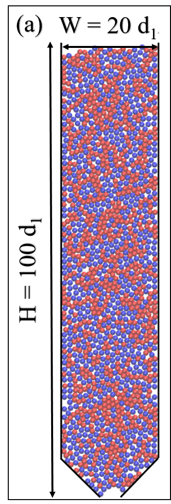
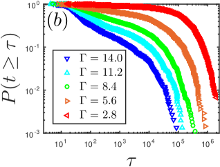
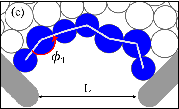
Figure 1: (color online) (a) Hopper geometry with width $W=20~{}d_{1}$ and height $H=100~{}d_{1}$ filled with a bidisperse mixture of $\sim 1600$ spherical grains. (b) Complementary cumulative distribution function $P(t\geq\tau)$ of the unclogging times for opening size $L=4.2~{}d_{1}$ and varying vibration amplitudes $\Gamma$. (c) Sample five-angle arch with a single opening angle $\phi_{1}$ marked. The lower walls are formed from static, closely spaced grains, size $d_{1}$, fixed at $45^{\circ}$ from the horizontal, and are vibrated vertically to unclog the flow.

Using Molecular Dynamics simulations Plimpton (1995); *LAMMPS of hopper flows, we show that the dynamics of arch shapes are well described by a continuous time random walk (CTRW) in which the vibrations activate transitions between locally stable arch shapes. Reminiscent of trap models of the glass transition Monthus and Bouchaud (1996), this CTRW is characterized by a broad distribution of waiting times that leads to ergodicity breaking Golding and Cox (2006); Lubelski et al. (2008); He et al. (2008); Jeon and Metzler (2010); Miyaguchi and Akimoto (2011); *Miyaguchi2013; Tabei et al. (2013).

Numerical Simulations

We perform Molecular Dynamics simulations based on LAMMPS Plimpton (1995); *LAMMPS using the quasi two-dimensional (2D) hopper geometry shown in Fig 1. A $50-50$ mixture of bidisperse spheres with diameter ratio $1:1.2$ were randomly distributed within the body of the hopper, allowed to settle under gravity, then flow until a clog develops. We excluded clogged configurations with less than 600 grains remaining in the hopper to ensure a grain depth of at least 1.5 times the hopper width. The ensemble of clogged states generated using this protocol (further details in SI ) were subjected to vibrations to unclog the flow. The inclined walls at the base of the hopper were displaced vertically at fixed frequency $f=10~{}(g/d_{1})^{1/2}$, and varying amplitudes $A=1\textendash 5\times 10^{-3}~{}d_{1}$. The vibration strength is characterized by a root-mean-square acceleration, $\Gamma=\frac{4\pi^{2}f^{2}A}{\sqrt{2}}$ that falls in the range of $\Gamma=2.8\textendash 14$ in units of the gravitational acceleration $g$. The initiation of flow was observed to be caused by arch failures except in rare cases where the arch slides out through the opening before collapsing.

The unclogging time is defined as the time elapsed from the start of the vibrations to the first time the center of any grain exits the outlet. The probability distribution function (PDF), $p(t;\Gamma,L)$, and the complementary cumulative distribution function (CCDF), $P(\tau;\Gamma,L)=\int_{\tau}^{\infty}p(t;\Gamma,L)dt$, are estimated from these measurements. All times, in results presented below, are quoted in units of the vibration period $T_{vib}=f^{-1}$. The CCDF is estimated directly by plotting the fraction of all measured unclogging times greater than or equal to each recorded time $\tau_{i}$ Newman (2005). The distributions were constructed from ensembles with $N=1744,1389,2718,1506,{\rm and}~{}1469$ different arches for $\Gamma=2.8,5.6,8.4,11.2,14.0$, respectively.

The CCDF in Fig. 1(b) demonstrates that vibrating the hopper produces broad distributions of unclogging times that are sensitive to the strength of the driving. As the vibration amplitude is reduced, the CCDF becomes broader, indicating an increase in the frequency of arch-breaking events occurring at longer times. The mean unclogging time grows from $\langle t\rangle=$1.58\text{\times}{10}^{3}$$ for $\Gamma=14.0$, to $\langle t\rangle=$2.5\text{\times}{10}^{5}$$ for $\Gamma=2.8$. The shape of the CCDF is characterized by three distinct regions: (i) an initial, fast decay characterizing arches that break quickly, (ii) a slower decay and broad plateau region extending over several decades, which crosses over to (iii) another fast decay characterized by a maximum unclogging time. For the smallest amplitude, $\Gamma=2.8$, $11$ out of $N=1744$ arches remained clogged for longer than the maximum simulation time tested $T_{sim}=$2\text{\times}{10}^{6}$$. Thus the shape of the CCDF can only be estimated up to $T_{sim}$ for this amplitude. In all other cases, the simulation time was sufficient to break all the arches. These characteristics are similar to those observed in experiments, except that the experiments report a pure power law tail Lozano et al. (2015).

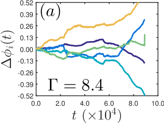
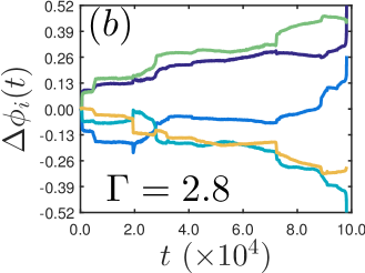
Figure 2: (color online) Time series of changes to the arch opening angles for two distinct five-angle arches ($N_{\phi}=5$) unclogged using vibration amplitudes $\Gamma=8.4$ (a) and $\Gamma=2.8$ (b). $\Delta\phi_{i}(t)$ indicates the change in radians from each of the initial opening angle values. The unclogging times are $t=89,107$ $(a)$ and $t=98,211$ $(b)$. The different angles within the arch (different colors within a panel) show correlated evolution in time. The arches usually undergo a series of reconfigurations, somtimes with changes to the angles as large as $30^{\circ}=0.52~{}rad$.

Arch Shape Dynamics

Since the distribution of unclogging times showed only a weak dependence on the opening size $L$ for our hopper geometry SI , we analyze the arch dynamics in detail for a single opening size $L=4.2~{}d_{1}$. The clogging arch is identified as the lowest chain of $N_{g}$ grains spanning the distance between the outlet walls. The shape of the arch is parameterized by $N_{\phi}=N_{g}-2$ opening angles $\phi_{i}(t)$ (Fig. 1). At $\L=4.2$, arches with $N_{\phi}=3,4,{\rm and}~{}5$ dominated the ensemble SI .

The dynamical response of an arch to the vibration is observed to be a correlated motion of the opening angles. Typical examples of the time evolution of $\phi_{i}(t)$ are shown in Fig. 2. (More examples in SI ). Characterizing the arch shape by the vector of opening angles $|{\phi(t)}\rangle=(\phi_{1}(t),..,\phi_{N_{\phi}}(t))$, we find that $|{\phi(t)}\rangle$ performs a “random walk” in the space of locally stable arch shapes, where each stable shape is characterized by a reconfiguration time that leads to a “waiting time” before the next step in the random walk. The dynamics of the clogging arch can thus be best described by a CTRW with a distribution, $\psi(t)$, of waiting times. The random environment created by the grains above the arch, including weak and strong force-bearing networks Tang et al. (2009); Hidalgo et al. (2013) is likely responsible for the broad distribution of waiting times. Since a precise definition and direct measurement of these waiting times was not feasible, we infer the features of the waiting time distribution by examining the time and ensemble averages of the mean squared displacement (MSD) of the arch angle vectors.

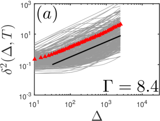
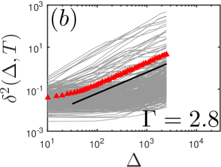
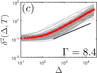
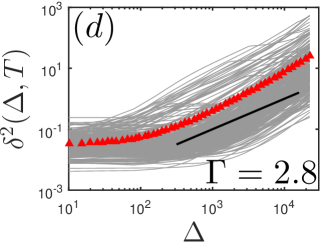
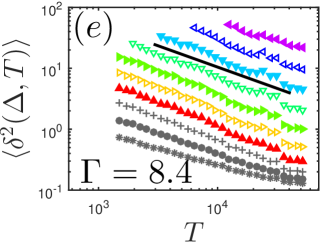
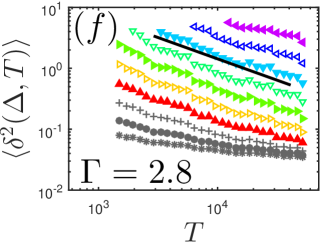
Figure 3: (color online) (a), (b), (c), (d): Time-averaged mean-squared displacements (TAMSD), $\delta^{2}(\Delta,T)$ and their ensemble average, $\langle\delta^{2}(\Delta,T)\rangle$ ( $\filledmedtriangleup$) shown for two sets of five-angle arches unclogged with vibration amplitudes $\Gamma=8.4$ (left) and $\Gamma=2.8$ (right). The ensembles are contrasted for an intermediate and a long total averaging time, $T=$5\text{\times}{10}^{3}$$ (a), (b) and $T=$4.5\text{\times}{10}^{4}$$ (c), (d). The ensembles include all arches that have survived until T or longer. The black lines show a linear slope $\sim\Delta$, the expected slope for a subdiffusive CTRW with a power law waiting time distribution. (e), (f): Scaling of $\langle\delta^{2}(\Delta,T)\rangle$ for both sets of arches. The different symbols show $\langle\delta^{2}(\Delta,T)\rangle$ evaluated for fixed values of the lag time $\Delta=24$ ( $\ast$), $\Delta=44$ ( $\bullet$), $\Delta=81$ ( $\plus$), $\Delta=149$ ( $\filledmedtriangleup$), $\Delta=272$ ( $\medtriangleright$), $\Delta=496$ ( $\filledmedtriangleright$), $\Delta=904$ ( $\medtriangledown$), $\Delta=1649$ ( $\filledmedtriangledown$), $\Delta=3007$ ( $\medtriangleleft$), $\Delta=5,484$ ( $\filledmedtriangleleft$). The black line indicates a T dependence $\sim T^{-0.7=-1+0.3}$.

TAMSD and Ergodicity Breaking

The time-averaged mean-squared displacement (TAMSD) is a standard measure used to characterize random walksGolding and Cox (2006); Lubelski et al. (2008); Jeon and Metzler (2010); Tabei et al. (2013). For each arch, the TAMSD is defined as

$$\delta^{2}(\Delta,T)=\frac{1}{T-\Delta}\int_{0}^{T-\Delta}\langle{\delta\phi(t,\Delta)}|{\delta\phi(t,\Delta)}\rangle dt~{},$$

where $|{\delta\phi(t,\Delta)}\rangle\equiv|{{\phi}(t+\Delta)}\rangle-|{{\phi}(t)}\rangle$, $\Delta$ is the lag time, and $T$ is the total time elapsed since the initiation of vibration. Properties of the underlying stochastic process can be inferred from the behavior of the ensemble-averaged TAMSD, $\langle\delta^{2}(\Delta,T)\rangle$, where the angular brackets indicate an average over a set of arches of the same size. In a CTRW, the TAMSD are random variables He et al. (2008). Thus, $\langle\delta^{2}(\Delta,T)\rangle$ and the ensemble-averaged mean-squared displacement (MSD), without any time averaging, are not necessarily identical. For sets of arches of the same size that are unclogged at the same amplitude, the MSD is calculated as

$$\langle\phi^{2}(t)\rangle=\frac{1}{N(t)}\sum_{i=1}^{i=N(t)}\Delta\vec{\phi}_{i}(t)\cdot\Delta\vec{\phi}_{i}(t)~{},$$

where the index $i$ indicates individual arches SI .

For a simple random walk, the $\delta^{2}(\Delta,T)$ are narrowly distributed around their mean $\langle\delta^{2}(\Delta,T)\rangle$, and for large T, the TAMSD for a single walker approaches the ensemble-averaged MSD: $\delta^{2}(\Delta,T\rightarrow\infty)=\langle\phi^{2}(t=\Delta)\rangle$. The class of CTRWs, characterized by a power law, $\psi(t)=t^{-\alpha+1}~{},t\rightarrow\infty$, with $0<\alpha<1$, is known to break ergodicity with time averages being different from ensemble averages Lubelski et al. (2008); He et al. (2008). $\langle\phi^{2}(t)\rangle$ is subdiffusive with an anomalous exponent $\alpha$: $\langle\phi^{2}(t)\rangle\propto t^{\alpha}$ (see Klafter and Sokolov (2011)). However, $\langle\delta^{2}(\Delta,T)$ is diffusive in $\Delta$, with the scaling form $\langle\delta^{2}(\Delta,T)\rangle\sim\frac{\Delta}{T^{1-\alpha}}$ $(\Delta<<T)$ Lubelski et al. (2008); He et al. (2008); Klafter and Sokolov (2011); Miyaguchi and Akimoto (2011); *Miyaguchi2013. We observe both a subdiffusive MSD SI , and a diffusive growth of $\langle\delta^{2}(\Delta,T)\rangle$ in the arch dynamics.

Fig. 3 compares many $\delta^{2}(\Delta,T)$ and their ensemble average, $\langle\delta^{2}(\Delta,T)\rangle$ for two different sets of five-angle arches ($N_{\phi}=5$) subjected to vibration amplitudes $\Gamma=8.4$ and $\Gamma=2.8$. These amplitudes were chosen for the main analysis of the arch dynamics because their $p(t;\Gamma,L)$ differ significantly. In addition, there are a sufficient number of long-lived arches to provide adequate statistics for time and ensemble averaging SI . For $T=5000$, there is a broad scatter in $\delta^{2}(\Delta,T)$ around $\langle\delta^{2}(\Delta,T)\rangle$ at both values of $\Gamma$. This broad scatter is a clear signature of ergodicity breaking Lubelski et al. (2008); Jeon and Metzler (2010); Bewerunge et al. (2016). For the longer averaging time $T=45000$, the broad scatter is still clearly present at $\Gamma=2.8$. At $\Gamma=8.4$, however, there is an apparent narrowing of the distribution, which hints at a possible recovery of ergodicity for long enough trajectories. We will address this feature below in the context of the precise functional form of the waiting time distribution $\psi(t)$ and its connection to the resulting unclogging time distribution in Fig 5. It is also clear that the $\Delta$ scaling of $\langle\delta^{2}(\Delta,T)\rangle$ emerges only for $\Delta>\Delta_{0}\approx 10^{2}$. The CTRW model is thus able to capture the dynamics of the arches at time scales much longer than a vibration period.

In Fig. 3 $(e)$ and $(f)$, we plot $\langle\delta^{2}(\Delta,T)\rangle$ as a function of $T$ for five-angle arches at $\Gamma=8.4$ and $\Gamma=2.8$, at different values of $\Delta$. As seen from the figure, $\langle\delta^{2}(\Delta,T)\rangle$ follows the predicted scaling form $\langle\delta^{2}(\Delta,T)\rangle\sim\frac{\Delta}{T^{1-\alpha}}$ with $\alpha\simeq 0.3$ for the range $\Delta_{0}<\Delta<<T$. Within statistical errors, results for both the amplitudes were consistent with this exponent. Comparing the two amplitudes (vertical axes in Fig. 3 $(e)$ and $(f)$), $\langle\delta^{2}(\Delta,T)\rangle$ shows a change in magnitude of $\approx 10$, which indicates a decrease in the magnitude of the effective diffusion coefficient $D_{\alpha}$ as the amplitude decreases from $\Gamma=8.4$ to $\Gamma=2.8$. The same reduction in magnitude is also present in the ensemble-averaged MSD $\langle\phi^{2}(t)\rangle$ SI

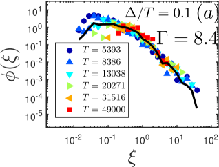
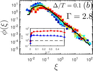
Figure 4: (color online) Distributions $\phi(\xi)$ of the normalized TAMSD $\xi=\frac{\delta^{2}}{\langle\delta^{2}\rangle}$ for $\Gamma=8.4$ $(a)$ and for $\Gamma=2.8$ $(b)$. The shapes of the distributions were found to depend on the ratio $\Delta/T$, and are shown here for $\Delta/T=0.1$ and different $T$ values given in the legend, which are the same for both plots. The averaged $\phi(\xi)$, black solid line, is used to compute the EB at $\Delta/T=0.1$. Inset to (b): EB parameter, $\langle\xi^{2}\rangle-\langle\xi\rangle^{2}$ for amplitudes $\Gamma=2.8$ ( $\bullet$) and $\Gamma=8.4$ ( $\filledmedtriangleup$) as a function of $\Delta/T$, computed using averaged $\phi(\xi)$ over a range of $\Delta/T$ SI . The EB parameter is roughly constant in the range $\Delta/T=0.1\textendash 0.4$. The dashed black line indicates the expected EB value for a power law $\psi(t)$ with $\alpha=0.3$.

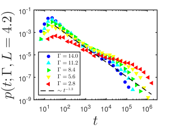
Figure 5: (color online) Probability distribution functions $p(t;\Gamma,L))$ for the unclogging times measured for varying vibration strengths $\Gamma=2.8,5.6,8.4,11.2,14.0$. These distributions are seen to have a peak at short unclogging times, a broad, similar power-like like decay over an intermediate range of times, and finally an upper cutoff time scale at long times. The tails of the distribution show an increasingly dominant plateau, indicating the weight in the unclogging time distributions is being redistributed from shorter to longer unclogging times.

Effects of vibration amplitude

A CTRW differs crucially from a simple random walk in that the $\delta^{2}(\Delta,T)$ are random variables Lubelski et al. (2008); He et al. (2008); Klafter and Sokolov (2011). The properties of this stochastic variable are characterized by the distribution $\phi(\xi)$ of the scaled variable $\xi(\Delta,T)=\delta^{2}(\Delta,T)/\langle\delta^{2}\rangle(\Delta,T)$. For a pure random walk, this distribution approaches a delta function $\delta(\xi-1)$ at large $T$. In contrast, for a CTRW with a power law distribution of waiting times, $\phi(\xi)$ approaches a universal form parametrized by the power-law exponent $\alpha$ at large $\Delta$ and $T$ He et al. (2008). The form of $\phi(\xi)$ provides information about the underlying stochastic process beyond that contained in the ensemble average $\langle\delta^{2}(\Delta,T)\rangle$. In particular, the variance $\rm{EB}\equiv\langle\xi^{2}\rangle-\langle\xi\rangle^{2}$ provides a quantitative measure of ergodicity breaking He et al. (2008).

We measured the distribution $\phi(\xi)$ for the same ensemble of arches that were considered in the TAMSD study. For $\Gamma=8.4~{}\rm{and}~{}2.8$, we find that $\phi(\xi)$ depends only on the ratio $\Delta/T$ SI . In Fig. 4, we plot $\phi(\xi)$, and EB, obtained by averaging over a large range of both $\Delta$ and $T$, as a function of $\Delta/T$. For $\Delta/T=0.1\textendash 0.4$, the form of the distribution and its variance are roughly independent of $\Delta/T$. Remarkably, this value depends sensitively on $\Gamma$, with an average value of $40$ for $\Gamma=8.4$ and $6$ for $\Gamma=2.8$. Both these values are much larger than the asymptotic prediction ($EB=0.8$) for a pure power law $\psi(t)$ with $\alpha=0.3$ He et al. (2008). It is clear that $\phi(\xi)$ for the arch dynamics has significantly more weight at $\xi>>1$ than expected from a power-law CTRW, and a concomitant shift in the peak to $\xi<1$ to maintain a mean of unity.

Both $\phi(\xi)$ and the unclogging time distribution $p(t;\Gamma,L)$ should be sensitive indicators of the form of $\psi(t)$ governing the transitions between locally stable arch structures. Since $\phi(\xi)$ indicates a larger sample-to-sample heterogeneity of the arch dynamics than expected for a power-law CTRW consistent with the scaling of $\langle\delta^{2}(\Delta,T)\rangle$, $p(t;\Gamma,L)$ should also show a corresponding deviation from a pure power law behavior. As seen in Fig 5, the distributions $p(t;\Gamma,L)$ are indeed broader than that expected from $\psi(t)\propto t^{-\alpha+1}$ with $\alpha=0.3$. As $\Gamma$ is reduced, weight in the distribution is shifted from short times to long times, consistent with the changes of $\phi(\xi)$ with $\Gamma$. We can, therefore, conclude that (a) the waiting-time distribution characterizing the arch dynamics is broader than a power-law, and (b) as the vibration amplitude is decreased, the ensemble of arches becomes increasingly dominated by ones that live longer than expected from a power-law. We note, however, that there is a clear cutoff in the unclogging time distribution that grows as $\Gamma$ is reduced (CCDF in Fig. 1).

The distribution of first passage times of a CTRW has an upper cutoff only if it occurs in a bounded volume Redner (2001) and if, in addition, $\psi(t)$ has a large timescale cutoff Metzler and Klafter (2004); Miyaguchi and Akimoto (2011); *Miyaguchi2013. The space of arch-angles is indeed bounded. For any finite system, a cutoff in $\psi(t)$ is also to be expected since arches will ultimately break or simply fall out of the hopper. Finite-size effects have been studied in detail for power-law CTRWsMiyaguchi and Akimoto (2011); *Miyaguchi2013. In experiments, the unclogging time distributionsZuriguel et al. (2014); Lozano et al. (2015) do not seem to have a characteristic cutoff time, which possibly reflects the fact that this time is much larger than the duration of the experiment.

Conclusions

Detailed analysis of the dynamics of arch shapes in response to vibrations demonstrates that clogging arches break ergodicity. The arches evolve in a landscape of locally stable shapes reminiscent of trap models Monthus and Bouchaud (1996) with anomalously broad distribution of trap depths. Mapping the dynamics to a CTRW, we quantify the degree of ergodicity breaking and show that it increases with decreasing vibration amplitude. This mechanism explains the broad distribution of unclogging times observed in our numerical simulations, and experiments Zuriguel et al. (2014); Lozano et al. (2015). We find that the distributions are broader than expected from a power-law distribution of waiting times, which in turn follows from an exponential distribution of trap depths Monthus and Bouchaud (1996). Recent analysis of experiments Zur in terms of a trap model indicates that the distribution of trap depths is a stretched exponential. Such a distribution could lead to the strong ergodicity breaking observed in the simulations. It would be interesting to measure the extent of ergodicity breaking in the vibrated-hopper experiments.

Acknowledgements: The work of CM and BC has been supported by NSF-DMR 1409093 as well as the Brandeis IGERT program. SKB thanks Narayanan Menon and Rama Govindarajan for their support, and acknowledges funding from TCIS Hyderabad, ICTS Bangalore, the APS-IUSSTF for a travel grant and NSF-DMR 120778 and NSF-DMR 1506750 at UMass Amherst. We would like to thank Iker Zuriguel, Ángel Garcimartín, Aparna Baskaran, and Kabir Ramola for helpful discussions and comments.

References

- Zuriguel (2014) I. Zuriguel, Pap. Phys. 6, 13 (2014).
- Zuriguel et al. (2014) I. Zuriguel, D. R. Parisi, R. C. Hidalgo, C. Lozano, A. Janda, P. A. Gago, J. P. Peralta, L. M. Ferrer, L. A. Pugnaloni, E. Clément, D. Maza, I. Pagonabarraga, and A. Garcimartín, Sci. Rep. 4 (2014).
- Helbing et al. (2000) D. Helbing, I. Farkas, and T. Vicsek, Nature 407, 487 (2000).
- Thomas and Durian (2015) C. E. Thomas and D. E. Durian, Phys. Rev. Lett. 114, 1 (2015).
- To et al. (2001) K. To, P. Y. Lai, and H. K. Pak, Phys. Rev. Lett. 86, 71 (2001).
- Zuriguel et al. (2005) I. Zuriguel, A. Garcimartín, D. Maza, L. A. Pugnaloni, J. M. Pastor, and L. Plata, Phys. Rev. E - Stat. Nonlinear, Soft Matter Phys. 71, 1 (2005).
- Janda et al. (2008) A. Janda, I. Zuriguel, A. Garcimartín, L. A. Pugnaloni, and D. Maza, EPL Europhys. Lett. 84, 44002 (2008).
- Tang et al. (2009) J. Tang, S. Sagdiphour, R. Behringer, M. Nakagawa, and S. Luding, in AIP Conference Proceedings, Vol. 1145 (AIP, 2009) pp. 515–518.
- Kondic (2014) L. Kondic, Granul. Matter 16, 235 (2014).
- Lozano et al. (2015) C. Lozano, I. Zuriguel, and A. Garcimartín, Phys. Rev. E 91 (2015).
- Janda et al. (2009) A. Janda, D. Maza, A. Garcimartin, E. Kolb, J. Lanuza, and E. Clement, EPL Europhys. Lett. 87, 24002 (2009).
- Mankoc et al. (2009) C. Mankoc, A. Garcimartín, I. Zuriguel, D. Maza, and L. A. Pugnaloni, Phys. Rev. E 80 (2009).
- Lozano et al. (2012) C. Lozano, G. Lumay, I. Zuriguel, R. C. Hidalgo, and A. Garcimartin, Phys. Rev. Lett. 109, 1 (2012).
- Hidalgo et al. (2013) R. C. Hidalgo, C. Lozano, I. Zuriguel, and A. Garcimartin, Granul. Matter 15, 841 (2013).
- Plimpton (1995) S. Plimpton, J. Comput. Phys. 117, 1 (1995).
- (16) Http://lammps.sandia.gov.
- Monthus and Bouchaud (1996) C. Monthus and J.-P. Bouchaud, J. Phys. A. Math. Gen. 29, 3847 (1996).
- Golding and Cox (2006) I. Golding and E. C. Cox, Phys. Rev. Lett. 96 (2006).
- Lubelski et al. (2008) A. Lubelski, I. M. Sokolov, and J. Klafter, Phys. Rev. Lett. 100 (2008).
- He et al. (2008) Y. He, S. Burov, R. Metzler, and E. Barkai, Phys. Rev. Lett. 101 (2008).
- Jeon and Metzler (2010) J.-H. Jeon and R. Metzler, J. Phys. A Math. Theor. 43 (2010).
- Miyaguchi and Akimoto (2011) T. Miyaguchi and T. Akimoto, Phys. Rev. E - Stat. Nonlinear, Soft Matter Phys. 83 (2011).
- Miyaguchi and Akimoto (2013) T. Miyaguchi and T. Akimoto, Phys. Rev. E - Stat. Nonlinear, Soft Matter Phys. 87 (2013).
- Tabei et al. (2013) S. M. Tabei, S. Burov, H. Y. Kim, A. Kuznetsov, T. Huynh, J. Jureller, L. H. Philipson, A. R. Dinner, and N. F. Scherer, Proc Natl Acad Sci U S A 110, 4911 (2013).
- (25) Please see supplementary material at [URL will be inserted by publisher] for details on the LAMMPS simulations, the TAMSD averaging procedure, and samples of the arch dynamics.
- Newman (2005) M. E. Newman, Contemp. Phys. 46, 323 (2005).
- Klafter and Sokolov (2011) J. Klafter and I. Sokolov, First Steps in Random Walks: From Tools to Applications (OUP Oxford, 2011).
- Bewerunge et al. (2016) J. Bewerunge, I. Ladadwa, F. Platten, C. Zunke, A. Heuer, and S. U. Egelhaaf, Phys. Chem. Chem. Phys. 18, 18887 (2016).
- Redner (2001) S. Redner, A Guide to First-Passage Processes, A Guide to First-passage Processes (Cambridge University Press, 2001).
- Metzler and Klafter (2004) R. Metzler and J. Klafter, J. Phys. A. Math. Gen. 37 (2004).
- (31) A. Nicolas, A. Garcimartín, I. Zuriguel, “A Trap Model for Clogging and Unclogging Granular Hopper Flows”, Private Communication, In preparation.