The Complexity of Finding Small Separators in Temporal Graphs

Abstract

Temporal graphs are graphs with time-stamped edges. We study the problem of finding a small vertex set (the separator) with respect to two designated terminal vertices such that the removal of the set eliminates all temporal paths connecting one terminal to the other. Herein, we consider two models of temporal paths: paths that pass through arbitrarily many edges per time step (non-strict) and paths that pass through at most one edge per time step (strict). Regarding the number of time steps of a temporal graph, we show a complexity dichotomy (NP-hardness versus polynomial-time solvability) for both problem variants. Moreover we prove both problem variants to be NP-complete even on temporal graphs whose underlying graph is planar. We further show that, on temporal graphs with planar underlying graph, if additionally the number of time steps is constant, then the problem variant for strict paths is solvable in quasi-linear time. Finally, we introduce and motivate the notion of a temporal core (vertices whose incident edges change over time). We prove that the non-strict variant is fixed-parameter tractable when parameterized by the size of the temporal core, while the strict variant remains NP-complete, even for constant-size temporal cores.

1 Introduction

In complex network analysis, it is nowadays very common to have access to and process graph data where the interactions among the vertices are time-stamped. When using static graphs as a mathematical model, the dynamics of interactions are not reflected and important information of the data might not be captured. Temporal graphs address this issue. A temporal graph is, informally speaking, a graph where the edge set may change over a discrete time interval, while the vertex set remains unchanged. Having the dynamics of interactions represented in the model, it is essential to adapt definitions such as connectivity and paths to respect temporal features. This directly affects the notion of separators in the temporal setting. Vertex separators are a fundamental primitive in static network analysis and it is well-known that they can be computed in polynomial time (see, e.g., proof of [1, Theorem 6.8]). In contrast to the static case, Kempe et al. [27] showed that in temporal graphs it is NP-hard to compute minimum separators.

Temporal graphs are well-established in the literature and are also referred to as time-varying [29] and evolving [17] graphs, temporal networks [26, 27, 32], link streams [28, 38], multidimensional networks [9], and edge-scheduled networks [8]. In this work, we use the well-established model in which each edge has a time stamp [9, 26, 2, 24, 27, 32, 4]. Assuming discrete time steps, this is equivalent to a sequence of static graphs over a fixed set of vertices [33]. Formally, we define a temporal graph as follows.

Definition 1.1 (Temporal Graph).

An (undirected) temporal graph $\bm{G}=(V,\bm{E},\tau)$ is an ordered triple consisting of a set $V$ of vertices, a set $\bm{E}\subseteq\binom{V}{2}\times\{1,\dots,\tau\}$ of time-edges, and a maximal time label $\tau\in\mathds{N}$.

See Figure 1 for an example with $\tau=4$, that is, a temporal graph with four time steps, also referred to as layers. The static graph obtained from a temporal graph $\bm{G}$ by removing the time stamps from all time-edges we call the underlying graph of $\bm{G}$.

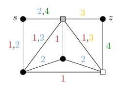
(a) A temporal graph $\bm{G}$.

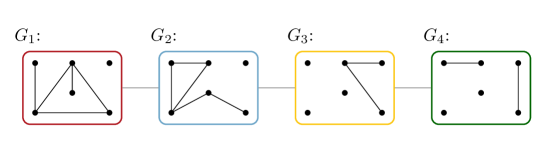
(b) Layers of $\bm{G}$.

Figure 1: Subfigure (a) shows a temporal graph $\bm{G}$ and subfigure (b) shows its four layers $G_{1},\ldots,G_{4}$. The gray squared vertex forms a strict temporal $(s,z)$-separator, but no temporal $(s,z)$-separator. The two squared vertices form a temporal $(s,z)$-separator.

Many real-world applications have temporal graphs as underlying mathematical model. For instance, it is natural to model connections in public transportation networks with temporal graphs. Other examples include information spreading in social networks, communication in social networks, biological pathways, or spread of diseases [26].

A fundamental question in temporal graphs, addressing issues such as connectivity [6, 32], survivability [29], and robustness [36], is whether there is a “time-respecting” path from a distinguished start vertex $s$ to a distinguished target vertex $z$. We provide a thorough study of the computational complexity of separating $s$ from $z$ in a given temporal graph.

Moreover, we study two natural restrictions of temporal graphs: (i) planar temporal graphs and (ii) temporal graphs with a bounded number of vertices incident to edges that are not permanently existing—these vertices form the so-called temporal core. Both restrictions are naturally motivated by settings e.g. occurring in (hierarchical) traffic networks. We also consider two very similar but still significantly differing temporal path models (both used in the literature), leading to two corresponding models of temporal separation.

Two path models.

We start with the introduction of the “non-strict” path model [27]. Given a temporal graph $\bm{G}=(V,\bm{E},\tau)$ with two distinct vertices $s,z\in V$, a temporal $(s,z)$-path of length $\ell$ in $\bm{G}$ is a sequence $P=((\{s=v_{0},v_{1}\},t_{1}),(\{v_{1},v_{2}\},t_{2}),\dots,(\{v_{\ell-1},v_{\ell}=z\},t_{\ell}))$ of time-edges in $\bm{E}$, where $v_{i}\neq v_{j}$ for all $i,j\in\{0,\ldots,\ell\}$ with $i\neq j$ and $t_{i}\leq t_{i+1}$ for all $i\in\{1,\ldots,\ell-1\}$. A vertex set $S$ with $S\cap\{s,z\}=\emptyset$ is a temporal $(s,z)$-separator if there is no temporal $(s,z)$-path in $\bm{G}-S:=(V\setminus S,\{(\{v,w\},t)\in\bm{E}\,|\,\mathopen{}v,w\in V\setminus S\},\tau)$. We are ready to state the central problem of our paper.

Temporal $(s,z)$-Separation

Input:	A temporal graph $\bm{G}=(V,\bm{E},\tau)$, two distinct vertices $s,z\in V$, and $k\in\mathds{N}$.
Question:	Does $\bm{G}$ admit a temporal $(s,z)$-separator of size at most $k$?

Our second path model is the “strict” variant. A temporal $(s,z)$-path $P$ is called strict if $t_{i}<t_{i+1}$ for all $i\in\{1,\dots,\ell-1\}$. In the literature, strict temporal paths are also known as journeys [2, 3, 33, 32]. A vertex set $S$ is a strict temporal $(s,z)$-separator if there is no strict temporal $(s,z)$-path in $\bm{G}-S$. Thus, our second main problem, Strict Temporal $(s,z)$-Separation, is defined in complete analogy to Temporal $(s,z)$-Separation, just replacing (non-strict) temporal separators by strict ones.

While the strict version of temporal separation immediately appears as natural, the non-strict variant can be viewed as a more conservative version of the problem. For instance, in a disease-spreading scenario the spreading speed might be unclear. To ensure containment of the spreading by separating patient zero ($s$) from a certain target ($z$), a temporal $(s,z)$-separator might be the safer choice.

Main results.

Table 1: Overview on our results. Herein, NP-c. abbreviates NP-complete, $n$ and $\bm{m}$ denote the number of vertices and time-edges, respectively, ${G}_{\downarrow}$ refers to the underlying graph of an input temporal graph. ^a (Thm. 3.1; W[1]-hard wrt. $k$) ^b (Thm. 3.6) ^c (Cor. 4.3) ^d (Prop. 4.5) ^e (Thm. 5.2)

	General		Planar ${G}_{\downarrow}$		Temporal core
	(Section 3)		(Section 4)		(Section 5)
$(s,z)$-Separation	$2\leq\tau\leq 4$	$5\leq\tau$	$\tau$ unbounded	$\tau$ constant	constant size
Temporal	NP-completea		NP-c.c	open	$n^{O(1)}+O(\bm{m}\log\bm{m})$ e
Strict Temporal	$\mathcal{O}(k\cdot\bm{m})$ b	NP-c.a	NP-c.c	$\mathcal{O}(\bm{m}\log\bm{m})$ d	NP-completea

Table 1 provides an overview on our results.

A central contribution is to prove that both Temporal $(s,z)$-Separation and Strict Temporal $(s,z)$-Separation are NP-complete for all $\tau\geq 2$ and $\tau\geq 5$, respectively, strengthening a result by Kempe et al. [27] (they show NP-hardness of both variants for all $\tau\geq 12$). For Temporal $(s,z)$-Separation, our hardness result is already tight. For the strict variant, we identify a dichotomy in the computational complexity by proving polynomial-time solvability of Strict Temporal $(s,z)$-Separation for $\tau\leq 4$. Moreover, we prove that both problems remain NP-complete on temporal graphs that have an underlying graph that is planar.

We introduce the notion of temporal cores in temporal graphs. Informally, the temporal core of a temporal graph is the set of vertices whose edge-incidences change over time. We prove that Temporal $(s,z)$-Separation is fixed-parameter tractable (FPT) when parameterized by the size of the temporal core, while Strict Temporal $(s,z)$-Separation remains NP-complete even if the temporal core is empty.

A particular aspect of our results is that they demonstrate that the choice of the model (strict versus non-strict) for a problem can have a crucial impact on the computational complexity of said problem. This contrasts with wide parts of the literature where both models were used without discussing the subtle but crucial differences in computational complexity.

Technical contributions.

To show the polynomial-time solvability of Strict Temporal $(s,z)$-Separation for $\tau\leq 4$, we prove that a classic separator result of Lovász et al. [30] translates to the strict temporal setting. This is surprising since many other results about separators in the static case do not apply in the temporal case. In this context, we also develop a linear-time algorithm for Single-Source Shortest Strict Temporal Paths, improving the running time of the best known algorithm due to Wu et al. [39] by a logarithmic factor.

We settle the complexity of Length-Bounded $(s,z)$-Separation on planar graphs by showing its NP-hardness, which was left unanswered by Fluschnik et al. [19] and promises to be a valuable intermediate problem for proving hardness results. In the hardness reduction for Length-Bounded $(s,z)$-Separation we introduce a grid-like, planarity-preserving vertex gadget that is generally useful to replace “twin” vertices which in many cases are not planarity-preserving and which are often used to model weights.

While showing that Temporal $(s,z)$-Separation is fixed-parameter tractable when parameterized by the size of the temporal core, we employ a case distinction on the size of the temporal core, and show that in the non-trivial case we can reduce the problem to Node Multiway Cut. We identify an “above lower bound parameter” for Node Multiway Cut that is suitable to lower-bound the size of the temporal core, thereby making it possible to exploit a fixed-parameter tractability result due to Cygan et al. [14].

Related work.

Our most important reference is the work of Kempe et al. [27] who proved that Temporal $(s,z)$-Separation is NP-hard. In contrast, Berman [8] proved that computing temporal $(s,z)$-cuts (edge deletion instead of vertex deletion) is polynomial-time solvable. In the context of survivability of temporal graphs, Liang and Modiano [29] studied cuts where an edge deletion only lasts for $\delta$ consecutive time stamps. Moreover, they studied a temporal maximum flow defined as the maximum number of sets of journeys where each two journeys in a set do not use a temporal edge within some $\delta$ time steps. A different notion of temporal flows on temporal graphs was introduced by Akrida et al. [3]. They showed how to compute in polynomial time the maximum amount of flow passing from a source vertex $s$ to a sink vertex $z$ until a given point in time.

The vertex-variant of Menger’s Theorem [31] states that the maximum number of vertex-disjoint paths from $s$ to $z$ equals the size of a minimum-cardinality $(s,z)$-separator. In static graphs, Menger’s Theorem allows for finding a minimum-cardinality $(s,z)$-separator via maximum flow computations. However, Berman [8] proved that the vertex-variant of an analogue to Menger’s Theorem for temporal graphs, asking for the maximum number of (strict) temporal paths instead, does not hold. Kempe et al. [27] proved that the vertex-variant of the former analogue to Menger’s Theorem holds true if the underlying graph excludes a fixed minor. Mertzios et al. [32] proved another analogue of Menger’s Theorem: the maximum number of strict temporal $(s,z)$-path which never leave the same vertex at the same time equals the minimum number of node departure times needed to separate $s$ from $z$, where a node departure time $(v,t)$ is the vertex $v$ at time point $t$.

Michail and Spirakis [34] introduced the time-analogue of the famous Traveling Salesperson problem and studied the problem on temporal graphs of dynamic diameter $d\in\mathds{N}$, that is, informally speaking, on temporal graphs where every two vertices can reach each other in at most $d$ time steps at any time. Erlebach et al. [16] studied the same problem on temporal graphs where the underlying graph has bounded degree, bounded treewidth, or is planar. Additionally, they introduced a class of temporal graphs with regularly present edges, that is, temporal graphs where each edge is associated with two integers upper- and lower-bounding consecutive time steps of edge absence. Axiotis and Fotakis [6] studied the problem of finding the smallest temporal subgraph of a temporal graph such that single-source temporal connectivity is preserved on temporal graphs where the underlying graph has bounded treewidth. In companion work, we recently studied the computational complexity of (non-strict) temporal separation on several other restricted temporal graphs [20].

2 Preliminaries

Let $\mathds{N}$ denote the natural numbers without zero. For $n\in\mathds{N}$, we use $[n]:=[1,n]=\{1,\ldots,n\}$.

Static graphs. We use basic notations from (static) graph theory [15]. Let $G=(V,E)$ be an undirected, simple graph. We use $V(G)$ and $E(G)$ to denote the set of vertices and set of edges of $G$, respectively. We denote by $G-V^{\prime}$ $:=(V\setminus V^{\prime},\{\{v,w\}\in E\,|\,\mathopen{}v,w\in V\setminus V^{\prime}\})$ the graph $G$ without the vertices in $V^{\prime}\subseteq V$. For $V^{\prime}\subseteq V$, $G[V^{\prime}]:=G-(V\setminus V^{\prime})$ denotes the induced subgraph of $G$ by $V^{\prime}$. A path of length $\ell$ is sequence of edges $P=(\{v_{1},v_{2}\},\{v_{2},v_{3}\},\dots,\{v_{\ell},v_{\ell+1}\})$ where $v_{i}\neq v_{j}$ for all $i,j\in[\ell+1]$ with $i\neq j$. We set $V(P)=\{v_{1},v_{2},\ldots,v_{\ell+1}\}$. Path $P$ is an $(s,z)$-path if $s=v_{1}$ and $z=v_{\ell+1}$. A set $S\subseteq V\setminus\{s,z\}$ of vertices is an $(s,z)$-separator if there is no $(s,z)$-path in $G-S$.

Temporal graphs. Let $\bm{G}=(V,\bm{E},\tau)$ be a temporal graph. The graph $G_{i}(\bm{G})=(V,E_{i}(\bm{G}))$ is called layer $i$ of the temporal graph $\bm{G}=(V,\bm{E},\tau)$ where $\{v,w\}\in E_{i}(\bm{G})\Leftrightarrow(\{v,w\},i)\in\bm{E}$. The underlying graph ${G}_{\downarrow}(\bm{G})$ of a temporal graph $\bm{G}=(V,\bm{E},\tau)$ is defined as ${G}_{\downarrow}(\bm{G}):=(V,{E}_{\downarrow}(\bm{G}))$, where ${E}_{\downarrow}(\bm{G})=\{e\,|\,\mathopen{}(e,t)\in\bm{E}\}$. (We write $G_{i}$, $E_{i}$, ${G}_{\downarrow}$, and ${E}_{\downarrow}$ for short if $\bm{G}$ is clear from the context.) For $X\subseteq V$ we define the induced temporal subgraph of $X$ by $\bm{G}[X]:=(X,\{(\{v,w\},t)\in\bm{E}\,|\,\mathopen{}v,w\in X\},\tau)$. We say that $\bm{G}$ is connected if its underlying graph ${G}_{\downarrow}$ is connected. For surveys concerning temporal graphs we refer to [10, 33, 26, 28, 25].

Regarding our two models, we have the following connection:

Lemma 2.1.

There is a linear-time computable many-one reduction from Strict Temporal $(s,z)$-Separation to Temporal $(s,z)$-Separation that maps any instance $(\bm{G}=(V,\bm{E},\tau),s,z,k)$ to an instance $(\bm{G}^{\prime}=(V^{\prime},\bm{E}^{\prime},\tau^{\prime}),s,z,k^{\prime})$ with $k^{\prime}=k$ and $\tau^{\prime}=2\cdot\tau$.

Proof.

Let $\mathcal{I}=(\bm{G}=(V,\bm{E},\tau),s,z,k)$ be an instance of Strict Temporal $(s,z)$-Separation. We construct an equivalent instance $\mathcal{I}^{\prime}=(\bm{G}^{\prime}=(V^{\prime},\bm{E}^{\prime},\tau^{\prime}=2\tau),s,z,k^{\prime}=k)$ in linear-time. Set $V^{\prime}=V\cup V_{E}$, where $V_{E}:=\{e_{(v,w),i},e_{(w,v),i}\,|\,\mathopen{}e\in\bm{E}\}$ is called the set of edge-vertices. Next, let $\bm{E}^{\prime}$ be initially empty. For each $(\{v,w\},t)\in\bm{E}$, add the time-edges $(\{v,e_{(v,w),t}\},2t-1),(\{e_{(v,w),t},w\},2t),(\{w,e_{(w,v),t}\},2t-1),(\{e_{(w,v),t},v\},2t)$ to $\bm{E}^{\prime}$. This completes the construction of $\bm{G}^{\prime}$. Note that this can be done in $\mathcal{O}(|V|+|\bm{E}|)$ time. It holds that $|V^{\prime}|=|V|+2\cdot|\bm{E}|$ and that $|\bm{E}^{\prime}|=4\cdot|\bm{E}|$.

We claim that $\mathcal{I}$ is a yes-instance if and only if $\mathcal{I}^{\prime}$ is a yes-instance.

$\Rightarrow$: Let $S$ be a temporal $(s,z)$-separator in $\bm{G}$ of size at most $k$. We claim that $S$ is also a temporal $(s,z)$-separator in $\bm{G}^{\prime}$. Suppose towards a contradiction that this is not the case. Then there is a temporal $(s,z)$-path $P$ in $\bm{G}^{\prime}-S$. Note that the vertices on $P$ alternated between vertices in $V$ and $V_{E}$. As each vertex in $V_{E}$ corresponds to an edge, there is a temporal $(s,z)$-path in $\bm{G}-S$ induced by the vertices of $V(P)\cap V$. This is a contradiction.

$\Leftarrow$: Observe that from any temporal $(s,z)$-separator, we can obtain a temporal $(s,z)$-separator of not larger size that only contains vertices in $V$. Let $S^{\prime}$ be a temporal $(s,z)$-separator in $\bm{G}^{\prime}$ of size at most $k$ only containing vertices in $S$. We claim that $S^{\prime}$ is also a temporal $(s,z)$-separator in $\bm{G}^{\prime}$. Suppose towards a contradiction that this is not the case. Then there is a temporal $(s,z)$ path $P$ in $\bm{G}-S^{\prime}$. Note that we can obtain a temporal $(s,z)$-path $P^{\prime}$ in $\bm{G}^{\prime}-S^{\prime}$ by adding for all consecutive vertices $v$, $w$, where $v$ appears before $w$ at time-step $t$ on $P$, the vertex $e_{(v,w),t}$. This is a contradiction. ∎

Throughout the paper we assume that the underlying graph of the temporal input graph $\bm{G}$ is connected and that there is no time-edge between $s$ and $z$. Furthermore, in accordance with Wu et al. [39] we assume that the time-edge set $\bm{E}$ is ordered by ascending time stamps.

2.1 The Maximum Label is Bounded in the Input Size

In the following, we prove that for every temporal graph in an input to (Strict) Temporal $(s,z)$-Separation, we can assume that the number of layers is at most the number of time-edges. Observe that a layer of a temporal graph that contains no edge is irrelevant for Temporal $(s,z)$-Separation. This also holds true for the strict case. Hence, we can delete such a layer from the temporal graph. This observation is formalized in the following two data reduction rules.

Reduction Rule 2.1.

Let $\bm{G}=(V,\bm{E},\tau)$ be a temporal graph and let $[t_{1},t_{2}]\subseteq[1,\tau]$ be an interval where for all $t\in[t_{1},t_{2}]$ the layer $G_{t}$ is an edgeless graph. Then for all $(\{v,w\},t^{\prime})\in\bm{E}$ where $t^{\prime}>t_{2}$ replace $(\{v,w\},t^{\prime})$ with $(\{v,w\},t^{\prime}-t_{2}+t_{1}-1)$ in $\bm{E}$.

Reduction Rule 2.2.

Let $\bm{G}=(V,\bm{E},\tau)$ be a temporal graph. If there is a non-empty interval $[t_{1},\tau]$ where for all $t^{\prime}\in[t_{1},\tau]$ the layer $G_{t^{\prime}}$ is an edgeless graph, then set $\tau$ to $t_{1}-1$.

We prove next that both reduction rules are exhaustively applicable in linear time.

Lemma 2.2.

Reduction Rules 2.1 and 2.2 do not remove or add any temporal $(s,z)$-path from/to the temporal graph $\bm{G}=(V,\bm{E},\tau)$ and can be exhaustively applied in $\mathcal{O}(|\bm{E}|)$ time.

Proof.

First we discuss Reduction Rule 2.1. Let $\bm{G}=(V,\bm{E},\tau)$ be a temporal graph, $s,z\in V$, $[t_{\alpha},t_{\beta}]\subseteq[\tau]$ be an interval where for all $t\in[t_{\alpha},t_{\beta}]$ the layer $G_{t}$ is an edgeless graph. Let $P=((e_{1},t_{1}),\dots,(e_{i},t_{i}),(e_{i+1},t_{j}),\dots,(e_{n},t_{n}))$ be a temporal $(s,z)$-path, and let $\bm{G}^{\prime}$ be the graph after we applied Reduction Rule 2.1 once on $\bm{G}$. We distinguish three cases.

1. If $t_{\beta}>t_{n}$, then no time-edge of $P$ is touched by Reduction Rule 2.1. Hence, $P$ also exists in $\bm{G}^{\prime}$.

2. If $t_{i}<t_{\alpha}<t_{\beta}<t_{i+1}$, then there is a temporal $(s,z)$-path $((e_{1},t_{1}),\dots,(e_{i},t_{i}),$ $(e_{i+1},t_{j}-t_{\beta}+t_{\alpha}-1),\dots,(e_{n},t_{n}-t_{\beta}+t_{\alpha}-1))$ in $\bm{G}^{\prime}$, because $t_{i}<t_{i+1}-t_{\beta}+t_{\alpha}-1$.

3. If $t_{\beta}<t_{1}$, then there is clearly a temporal $(s,z)$-path $((e_{1},t_{1}-t_{\beta}+t_{\alpha}-1),\dots,$ $(e_{n},t_{n}-t_{\beta}+t_{\alpha}-1))$ in $\bm{G}^{\prime}$

The other direction works analogously. We look at a temporal $(s,z)$-path in $\bm{G}^{\prime}$ and compute the corresponding temporal $(s,z)$-path in $\bm{G}$.

(a) Reduction Rule 2.1 is applicable

(b) Reduction Rule 2.1 is not applicable

Figure 2: Figure 2(a) shows a temporal graph where Reduction Rule 2.1 is applicable. In particular, layers $3,4,5,6$ are edgeless. Figure 2(b) shows the same temporal graph after Reduction Rule 2.1 was applied exhaustively.

Reduction Rule 2.1 can be exhaustively applied by iterating over the by time-edges $(e_{i},t_{i})$ in the time-edge set $E$ ordered by ascending labels until the first $t_{1},t_{2}$ with the given requirement appear. Set $x_{0}:=-t_{2}+t_{1}-1$. Then we iterate further over $E$ and replace each time-edge $(e,t)$ with $(e,t+x_{0})$ until the next $t_{1},t_{2}$ with the given requirement appear. Then we set $x_{1}=x_{0}-t_{2}+t_{1}-1$ and iterate further over $\bm{E}$ and replace each time-edge $(e,t)$ with $(e,t+x_{1})$. We repeat this procedure until the end of $\bm{E}$ is reached. Since we iterate over $\bm{E}$ only once, this can be done in $\mathcal{O}(|\bm{E}|)$ time.

Reduction Rule 2.2 can be executed in linear time by iterating over all edges and taking the maximum label as $t_{1}$. Note that the sets $V$ and $\bm{E}$ remain untouched by Reduction Rule 2.2. Hence, the application of Reduction Rule 2.2 does not add or remove any temporal $(s,z)$-path. ∎

A consequence of Lemma 2.2 is that the maximum label $\tau$ can be upper-bounded by the number of time-edges and hence the input size.

Lemma 2.3.

Let $\mathcal{I}=(\bm{G}=(V,\bm{E},\tau),s,z,k)$ be an instance of (Strict) Temporal $(s,z)$-Separation. There is an algorithm which computes in $\mathcal{O}(|\bm{E}|)$ time an instance $\mathcal{I}^{\prime}=(\bm{G}^{\prime}=(V,\bm{E}^{\prime},\tau^{\prime}),s,z,k)$ of (Strict) Temporal $(s,z)$-Separation which is equivalent to $\mathcal{I}$, where $\tau^{\prime}\leq|\bm{E}^{\prime}|$.

Proof.

Let $\bm{G}=(V,\bm{E},\tau)$ be a temporal graph, where Reduction Rules 2.1 and 2.2 are not applicable. Then for each $t\in[\tau]$ there is a time-edge $(e,t)\in\bm{E}$. Thus, $\tau\leq\sum_{i=1}^{\tau}|\{(e,t)\in\bm{E}\,|\,\mathopen{}t=i\}|\leq|\bm{E}|$. ∎

3 Hardness Dichotomy Regarding the Number of Layers

In this section we settle the complexity dichotomy of both Temporal $(s,z)$-Separation and Strict Temporal $(s,z)$-Separation regarding the number $\tau$ of time steps. We observe that both problems are strongly related to the following NP-complete [11, 37] problem:

Length-Bounded $(s,z)$-Separation (LBS)

Input:	An undirected graph $G=(V,E)$, distinct vertices $s,z\in V$, and $k,\ell\in\mathds{N}$.
Question:	Is there a subset $S\subseteq V\setminus\{s,z\}$ such that $|S|\leq k$ and there is no $(s,z)$-path in $G-S$ of length at most $\ell$?

Length-Bounded $(s,z)$-Separation is NP-complete even if the lower bound $\ell$ for the path length is five [7] and W[1]-hard with respect to the postulated separator size [22]. We obtain the following, improving a result by Kempe et al. [27] who showed NP-completeness of Temporal $(s,z)$-Separation and Strict Temporal $(s,z)$-Separation for all $\tau\geq 12$.

Theorem 3.1.

Temporal $(s,z)$-Separation is NP-complete for every maximum label $\tau\geq 2$ and Strict Temporal $(s,z)$-Separation is NP-complete for every $\tau\geq 5$. Moreover, both problems are W[1]-hard when parameterized by the solution size $k$.

We remark that our NP-hardness reduction for Temporal $(s,z)$-Separation is inspired by Baier et al. [7, Theorem 3.9].

Proof.

To show NP-completeness of Temporal $(s,z)$-Separation for $\tau=2$ we present a reduction from the Vertex Cover problem where, given a graph $G=(V,E)$ and an integer $k$, the task is to determine whether there exists a set $V^{\prime}\subseteq V$ of size at most $k$ such that $G-V^{\prime}$ does not contain any edge.

Construction.

Let $(G=(V,E),k)$ be an instance of Vertex Cover. We say that $V^{\prime}\subseteq V$ is a vertex cover in $G$ of size $k$ if $|V^{\prime}|=k$ and $V^{\prime}$ is a solution to $(G=(V,E),k)$. We refine the gadget of Baier et al. [7, Theorem 3.9] and reduce from Vertex Cover to Temporal $(s,z)$-Separation. Let $\mathcal{I}:=(G=(V,E),k)$ be a Vertex Cover instance and $n:=|V|$. We construct a Temporal $(s,z)$-Separation instance $\mathcal{I}^{\prime}:=(\bm{G}^{\prime}=(V^{\prime},\bm{E}^{\prime},2),s,z,n+k)$, where $V^{\prime}:=V\cup\{s_{v},t_{v}:v\in V\}\cup\{s,z\}$ are the vertices and the time-edges are defined as

$$\begin{split}\bm{E}^{\prime}:=\ &\overbrace{\{(\{s,s_{v}\},1),(\{s_{v},v\},1),(\{v,z_{v}\},2),(\{z_{v},z\},2),(\{s,v\},2),(\{v,z\},1):v\in V\}}^{\text{vertex-edges}}\ \cup\\ &\underbrace{\{(\{s_{v},z_{w}\},1),(\{s_{w},z_{v}\},1):\{v,w\}\in E\}}_{\text{edge-edges}}.\end{split}$$

Note that $|V^{\prime}|=3\cdot n+2$, $|\bm{E}^{\prime}|=6\cdot|V^{\prime}|+2\cdot|E|$, and $\mathcal{I}^{\prime}$ can be computed in polynomial time. For each vertex $v\in V$ there is a vertex gadget which consists of three vertices $s_{v},v,z_{v}$ and six vertex-edges. In addition, for each edge $\{v,w\}\in E$ there is an edge gadget which consists of two edge-edges $\{s_{v},z_{w}\}$ and $\{z_{v},s_{w}\}$. See Figure 3 for an example.

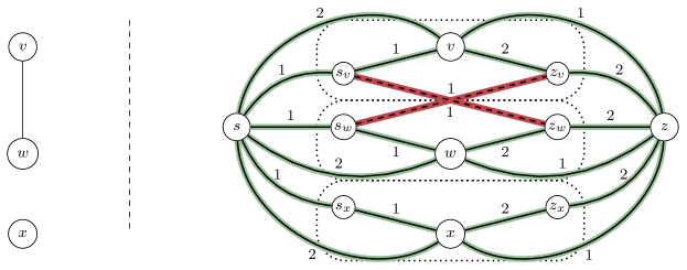
Figure 3: The Vertex Cover instance $(G,1)$ (left) and the corresponding Temporal $(s,z)$-Separation instance from the reduction of Theorem 3.1 (right). The edge-edges are dashed (red), the vertex-edges are solid (green), and the vertex gadgets are in dotted boxes.

Correctness.

We prove that $\mathcal{I}$ is a yes-instance if and only if $\mathcal{I}^{\prime}$ is a yes-instance.

$\Rightarrow$: Let $X\subseteq V$ be a vertex cover of size $k^{\prime}\leq k$ for $G$. We claim that $S:=(V\setminus X)\cup\{s_{v},z_{v}\,|\,\mathopen{}v\in X\}$ is a temporal $(s,z)$-separator. There are $|V|-|X|=n-k^{\prime}$ vertices not in the vertex cover $X$ and for each of them there is exactly one vertex in $S$. For each vertex in the vertex cover $X$ there are two vertices in $S$. Hence, $|S|=n-k^{\prime}+2k^{\prime}\leq n+k$.

First, we consider the vertex-gadget of a vertex $v\in V$. Note that in the vertex-gadget of $v$, there are two distinct temporal $(s,z)$-separators $\{v\}$ and $\{s_{v},z_{v}\}$. Hence, every temporal $(s,z)$-path in $\bm{G}^{\prime}-S$ contains an edge-edge. Second, let $e=\{v,w\}\in E$ and let $P_{e}$ and $P_{e}^{\prime}$ be the temporal $(s,z)$-paths which contain the edge-edges of edge-gadget of $e$ such that $V(P_{e})=\{s,s_{v},z_{w},z\}$ and $V(P_{e}^{\prime})=\{s,s_{w},z_{v},z\}$. Since $X$ is a vertex cover of $G$ we know that at least one element of $e$ is in $X$. Thus, $s_{v},z_{v}\in S$ or $s_{w},z_{w}\in S$, and hence neither $P_{e}$ nor $P_{e}^{\prime}$ exist in $\hat{G}-S$. It follows that $S$ is a temporal $(s,z)$-separator in $\bm{G}^{\prime}$ of size at most $n+k$, as there are no other temporal $(s,z)$-paths in $\bm{G}^{\prime}$.

$\Leftarrow$: Let $S$ be a temporal $(s,z)$-separator in $\bm{G}^{\prime}$ of size $\ell\leq n+k$ and let $v\in V$. Recall that there are two distinct temporal $(s,z)$-separators in the vertex gadget of $v$, namely $\{v\}$ and $\{s_{v},z_{v}\}$, and that all vertices in $V^{\prime}\setminus\{s,z\}$ are from a vertex gadget. Hence, $\ell$ is of the form $\ell=n+k^{\prime}\leq n+k$. We start with a preprocessing to ensure that for vertex gadget only one of these two separators are in $S$. Let $S_{v}=S\cap\{v,s_{v},z_{w}\}$. We iterate over $S_{v}$ for each $v\in V$:

1. If $S_{v}=\{v\}$ or $S_{v}=\{s_{v},z_{v}\}$ then we do nothing.

2. If $S_{v}=\{v,s_{v},z_{v}\}$ then we remove $v$ from $S$ and decrease $\ell$ by one. One can observe that all temporal $(s,z)$-paths which are visiting $v$ are still separated by $s_{v}$ or $w_{v}$.

3. If $S_{v}=\{v,s_{v}\}$ then we remove $v$ from $S$ and add $z_{v}$. One can observe that $S$ is still a temporal $(s,z)$-separator of size $\ell$ in $\bm{G}^{\prime}$.

4. If $S_{v}=\{v,z_{v}\}$ then we remove $v$ from $S$ and add $s_{v}$. One can observe that $S$ is still a temporal $(s,z)$-separator of size $\ell$ in $\bm{G}^{\prime}$.

That is a complete case distinction because neither $\{s_{v}\}$ nor $\{z_{v}\}$ separate all temporal $(s,z)$-paths in the vertex gadget in $v$. Now we construct a vertex cover $X$ for $G$ by taking $v$ into $X$ if both $s_{v}$ and $z_{v}$ are in $S$. Since there are $n$ vertex gadgets in $\bm{G}^{\prime}$ each containing either one or two vertices from $S$, it follows that $|X|=|S|-n=k^{\prime}\leq k$,

Assume towards a contradiction that $X$ is not a vertex cover of $G$. Then there is an edge $\{v,w\}\in E$ where $v,w\not\in X$. Hence, $s_{v},z_{v},s_{w},z_{w}\not\in S$ and $v,w\in S$. This contradicts the fact that $S$ is a temporal $(s,z)$-separator in $\bm{G}^{\prime}$, because $P=((\{s,s_{v}\},1),(\{s_{v},z_{w}\},1),$ $(\{z_{w},z\},2))$ is a temporal $(s,z)$-path in $\bm{G}^{\prime}-S$. It follows that $X$ is a vertex cover of $G$ of size at most $k$. ∎

Observation 3.2.

There is a polynomial-time reduction from LBS to Strict Temporal $(s,z)$-Separation that maps any instance $(G,s,z,k,\ell)$ of LBS to an instance $(\bm{G}=(G_{1},\ldots,G_{\ell}),s,z,k)$ with $G_{i}=G$ for all $i\in[\ell]$ of Strict Temporal $(s,z)$-Separation.

In the remainder of this section we prove that the bound on $\tau$ is tight in the strict case (for the non-strict case the tightness is obvious). This is the first case where we can observe a significant difference between the strict and the non-strict variant of our separation problem. In order to do so, we have to develop some tools which we need in subroutines. In Section 3.1, we introduce a common tool to study reachability in temporal graphs on directed graphs. This helps us to solve the Single-Source Shortest Strict Temporal Paths efficiently (Proposition 3.4). Note that this might be of independent interest since it improves known algorithms, see Section 3.2. Afterwards, in Section 3.3, we prove that Strict Temporal $(s,z)$-Separation can be solved in polynomial time, if the maximum label $\tau\leq 4$.

3.1 Strict Static Expansion

A key tool [8, 27, 32, 3, 39] is the time-expanded version of a temporal graph which reduces reachability and other related questions in temporal graphs to similar questions in directed graphs. Here, we introduce a similar tool for strict temporal $(s,z)$-paths. Let $\bm{G}=(V,\bm{E},\tau)$ be a temporal graph and let $V=\{v_{1},\dots,v_{n-2}\}\cup\{s,z\}$. For each $v\in\{v_{1},\dots,v_{n-2}\}$, we define the sets $\phi(v):=\{t,t+1\,|\,\mathopen{}t\in[\tau],\exists w:(\{v,w\},t)\in\bm{E}\}$ and $\vec{\phi}(v):=\{(t,t^{\prime})\in\phi(v)^{2}\,|\,\mathopen{}t<t^{\prime}\land\nexists t^{\prime\prime}\in\phi(v):t<t^{\prime\prime}<t^{\prime}\}$. The strict static expansion of $(\bm{G},s,z)$ is a directed acyclic graph $H:=(V^{\prime},A)$ where $V^{\prime}=\{s,z\}\cup\{u_{t,j}\,|\,\mathopen{}j\in[n-2]\land t\in\phi(v_{j})\}$ and $A=A^{\prime}\cup A_{s}\cup A_{z}\cup A_{\rm col}$, $A^{\prime}:=\{(u_{i,j},u_{i+1,j^{\prime}}),(u_{i,j^{\prime}},u_{i+1,j})\,|\,\mathopen{}(\{v_{j},v_{j^{\prime}}\},i)\in\bm{E}\}$, $A_{s}:=\{(s,u_{i+1,j})\,|\,\mathopen{}(\{s,v_{j}\},i)\in\bm{E}\}$, $A_{z}:=\{(u_{i,j},z)\,|\,\mathopen{}(\{v_{j},z\},i)\in\bm{E}\}$, and $A_{\rm col}:=\{(u_{t,j},u_{t^{\prime},j})\,|\,\mathopen{}(t,t^{\prime})\in\vec{\phi}(v_{j})\land j\in[n-2]\}$ (referred to as column-edges of $H$). Observe that each strict temporal $(s,z)$-path in $\bm{G}$ has a one-to-one correspondence to some $(s,z)$-path in $H$. We refer to Figure 4 for an example.

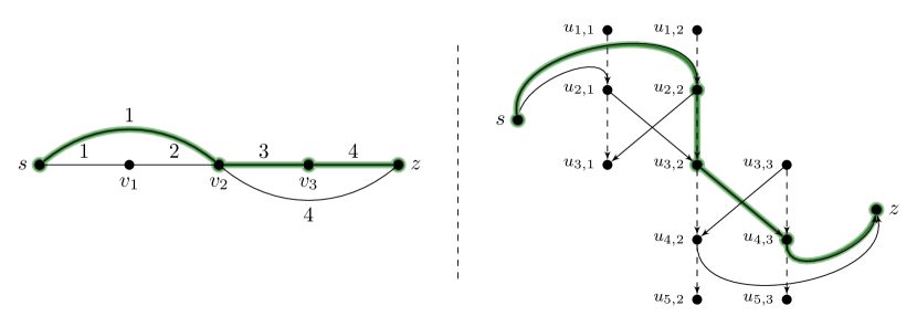
Figure 4: A temporal graph $\bm{G}$ (left) and the strict static expansion $H$ for $(\bm{G},s,z)$ (right). One strict temporal $(s,z)$-path in $\bm{G}$ and its corresponding $(s,z)$-path in $H$ are marked (green).

Lemma 3.3.

Let $\bm{G}=(V,\bm{E},\tau)$ be a temporal graph, where $s,z\in V$ are two distinct vertices. The strict static expansion for $(\bm{G},s,z)$ can be computed in $\mathcal{O}(|\bm{E}|)$ time.

Proof.

Let $\bm{G}=(V,\bm{E},\tau)$ be a temporal graph, where $V=\{v_{1},\dots,v_{n-2}\}\cup\{s,z\}$ and $s,z\in V$ are two distinct vertices. Note that $|V|\leq|\bm{E}|$ because $\bm{G}$ is connected. We construct the strict static expansion $H=(S,A)$ for $(\bm{G},s,z)$ as in four steps follows: First, we initiate for each $j\in[n-2]$ an empty linked list. Second, we iterate over the set $\bm{E}$ with non-decreasing labels and for each $(\{v_{j},v_{j^{\prime}}\},t)$:

1. Add $u_{t,j},u_{t+1,j},u_{t,j^{\prime}},u_{t+1,j^{\prime}}$ to $S$ if they do not already exist. If we added a vertex $u_{a,b}$ then we push $a$ to the $b$-th linked list.

2. Add $(u_{i,j},u_{i+1,j^{\prime}}),(u_{i,j^{\prime}},u_{i+1,j})$ to $A$.

This can be done in $\mathcal{O}(|\bm{E}|)$ time. Observe, that the two consecutive entries in the $i$-th linked list is an entry in $\vec{\phi}(v_{i})$. Third, we iterate over each linked list in increasing order to add the column-edges to $A$. Note that the sizes of all linked lists sum up to $\mathcal{O}(|\bm{E}|)$. Last, we add $s$ and $z$ to $S$ as well as the edges in $A_{s}$ and $A_{z}$ to $A$.

Note that the $|S|$ as well as $|A|$ can be upper-bounded by $\mathcal{O}(|\bm{E}|)$. We employed a constant number of procedures each running in $\mathcal{O}(|\bm{E}|)$ time. Thus, $H$ can be computed in $\mathcal{O}(|\bm{E}|)$ time. ∎

As a subroutine hidden in several of our algorithms, we need to solve the Single-Source Shortest Strict Temporal Paths problem on temporal graphs: find shortest strict paths from a source vertex $s$ to all other vertices in the temporal graph. Herein, we say that a strict temporal $(s,z)$-path is shortest if there is no strict temporal $(s,z)$-path of length $\ell^{\prime}<\ell$. Indeed, we provide a linear-time algorithm for this. We believe this to be of independent interest; it improves (with few adaptations to the model; for details see Section 3.2) previous results by Wu et al. [39], but in contrast to the algorithm of Wu et al. [39] our subroutine cannot be adjusted to the non-strict case.

Proposition 3.4.

Single-Source Shortest Strict Temporal Paths is solvable in $\Theta(|\bm{E}|)$ time.

The following proof makes use of a strict static expansion of a temporal graph. See Sec. 3.1 for more details.

Proof.

By Lemma 3.3, we compute the strict static expansion $H=(S,A)$ of $(\bm{G},s,z)$ in $\mathcal{O}(|\bm{E}|)$ time and define a weight function

$$\omega:A\rightarrow\{0,1\},(x,y)\mapsto\begin{cases}0,\text{if }(x,y)\text{ is a column-edge,}\\ 1,\text{otherwise.}\end{cases}$$

Observe that $H$ with $\omega$ is a weighted directed acyclic graph and that the weight of an $(s,z)$-path in $H$ with $\omega$ is equal to the length of the corresponding strict temporal $(s,z)$-path in $\bm{G}$. Hence, we can use an algorithm, which makes use of the topological order of $S$ on $H$, to compute for all $v\in S$ a shortest $(s,v)$-path in $H$ in $\mathcal{O}(|S|+|A|)=\mathcal{O}(|\bm{E}|)$ time (cf. Cormen et al. [12, Section 24.2]).

Now we iterate over $S$ and construct the shortest strict temporal $(s,w_{j})$-path in $\bm{G}$ from the shortest $(s,u_{t,j})$-path in $H$, where $w_{j}\in V$, $t\in\{1,\dots,\tau\}$ and $u_{t,j}\in S$. This can be done in $\mathcal{O}(|\bm{E}|)$ time because $|S|\in\mathcal{O}(|\bm{E}|)$. Consequently, the overall running time is $\mathcal{O}(|\bm{E}|)$. Since the shortest strict temporal $(s,z)$-path in $\bm{G}$ can have length $|\bm{E}|$, this algorithm is asymptotically optimal. ∎

3.2 Adaptation of Proposition 3.4 for the Model of Wu et al. [39]

Wu et al. [39] considered a model where the temporal graph is directed and a time-edge $e$ has a traversal time $\phi(e)\in\mathds{N}\cup\{0\}$. In the context of strict temporal path $\phi(e)$ is always one. They excluded the case where $\phi(e)=0$, but pointed out that their algorithms can be adjusted to allow $\phi(e)=0$. However, this is not possible for our algorithm, because then the strict static expansion can contain cycles. Hence, we assume that $\phi(e)>0$ for all directed time-edges $e$.

Let $\bm{G}=(V,\bm{E},\tau)$ be a directed temporal graph. We denote a directed time-edge from $v$ to $w$ in layer $t$ by $((v,w),t)\in\bm{E}$. First, we initiate $\tau$ many linked lists. Without loss of generality we assume that $\tau\leq|\bm{E}|$, see Lemma 2.3. Second, we construct a directed temporal graph $\bm{G}^{\prime}=(V^{\prime},\bm{E}^{\prime},\tau)$, where $V=V^{\prime}$ and $\bm{E}^{\prime}$ is empty in the beginning. Then we iterate over the time-edge set $\bm{E}$ by ascending labels. If $((v,w),t)\in\bm{E}$ has $\phi((v,w))=1$ then we add $((v,w),t)$ to $\bm{E}^{\prime}$. If $((v,w),t)\in\bm{E}$ has $\phi((v,w))>1$ then we add a new vertex $x_{(v,w)}$ to $V^{\prime}$ and add time-edge $((v,x_{(v,w)}),t)$ to $\bm{E}^{\prime}$ and $((x_{(v,w)},w),t^{\prime})$ to the $t^{\prime}$-th linked list, where $t^{\prime}=t+\phi((v,w))-1$. We call $((v,x_{(v,w)}),t)$ the original edge of $(v,w)$ and $((x_{(v,w)},w),t^{\prime})$ the connector edge of $(v,w)$. If we reach a directed time-edge with label $t$ for the first time, then we add all directed time-edges from the $t$-th linked list to $\bm{E}^{\prime}$. Observe that for each strict temporal $(s,z)$-path in $\bm{G}$ there is a corresponding strict temporal $(s,z)$-path in $\bm{G}^{\prime}$, additionally we have that $\bm{E}^{\prime}$ is ordered by ascending labels and that $\bm{G}^{\prime}$ can be constructed in $\mathcal{O}(|\bm{E}|)$ time.

To construct a strict static expansion for a directed temporal graph $\bm{G}$, we modify the edge set $A^{\prime}:=\{(u_{i,j},u_{i+1,j^{\prime}}),j^{\prime})\,|\,\mathopen{}((v_{j},v_{j^{\prime}}),i)\in\bm{E}\}$, where  $((v_{j},v_{j^{\prime}}),i)\in\bm{E}$. Finally, we adjust the weight function $\omega$ from the algorithm of Proposition 3.4 such that $\omega(e)=0$ if $e$ is a column-edges of correspond to a connector-edges, and $\omega(e)=\phi(e)$ otherwise. Observe that for a strict temporal $(s,z)$-path $P=(e_{1},\dots,e_{\ell})$ of traversal time $\sum_{i=1}^{\ell}\phi(e_{i})$ the corresponding $(s,z)$-path in the strict static expansion is of weight of the traversal time of $P$.

Our algorithm behind Theorem 3.6 executes the following steps:

1. As a preprocessing step, remove unnecessary time-edges and vertices from the graph.

2. Compute an auxiliary graph called directed path cover graph of the temporal graph.

3. Compute a separator for the directed path cover graph.

In the following, we explain each of the steps in more detail.

The preprocessing reduces the temporal graph such that it has the following properties. A temporal graph $\bm{G}=(V,\bm{E},\tau)$ with two distinct vertices $s,z\in V$ is reduced if (i) the underlying graph ${\bm{G}}_{\downarrow}$ is connected, (ii) for each time-edge $e\in\bm{E}$ there is a strict temporal $(s,z)$-path which contains $e$, and (iii) there is no strict temporal $(s,z)$-path of length at most two in $\bm{G}$. This preprocessing step can be performed in polynomial time:

Lemma 3.5.

Let $\mathcal{I}=(\bm{G}=(V,\bm{E},\tau),s,z,k)$ be an instance of Strict Temporal $(s,z)$-Separation. In $\mathcal{O}(k\cdot|\bm{E}|)$ time, one can either decide $\mathcal{I}$ or construct an instance $\mathcal{I}^{\prime}=(\bm{G}^{\prime}=(V^{\prime},\bm{E}^{\prime},\tau),s,z,k^{\prime})$ of Strict Temporal $(s,z)$-Separation such that $\mathcal{I}^{\prime}$ is equivalent to $\mathcal{I}$, $\bm{G}^{\prime}$ is reduced, $|V^{\prime}|\leq|V|$, $|\bm{E}^{\prime}|\leq|\bm{E}|$, and $k^{\prime}\leq k$.

The following proof makes use of a strict static expansion of a temporal graph. See Sec. 3.1 for more details.

Proof.

First, we remove all time-edges which are not used by a strict temporal $(s,z)$-path. Let $\mathcal{I}=(\bm{G}=(V,\bm{E},\tau)s,z,k)$ be an instance of Strict Temporal $(s,z)$-Separation. We execute the following procedure.

1. Construct the strict static expansion $H=(S,A)$ of $(\bm{G},s,z)$.

2. Perform a breadth-first search in $H$ from $s$ and mark all vertices in the search tree as reachable. Let $R(s)\subseteq S$ be the reachable vertices from $s$.

3. Construct $H^{\prime}:=(R(s),A^{\prime})$, where $A^{\prime}:=\{(w,v):(v,w)\in A\text{ and }v,w\in R(s)\}$. Observe that $H^{\prime}$ is the reachable part of $H$ from $s$, where all directed arcs change their direction.

4. If $z\notin R(s)$, then our instance $\mathcal{I}$ is a yes-instance.

5. Perform a breadth-first search from $z$ in $H^{\prime}$ and mark all vertices in the search tree as reachable. Let $R(z)\subseteq R(s)$ be the reachable set of vertices from $z$. In the graph $H[R(s)\cap R(z)]=H[R(z)]$, all vertices are reachable from $s$ and from each vertex the vertex $z$ is reachable.

6. Output the temporal graph $\bm{G}^{\prime}:=(V^{\prime},\bm{E}^{\prime},\tau)$, where  $V^{\prime}:=\{v_{i}\in V\,|\,\mathopen{}\exists j:x_{j,i}\in R(z)\}$ and $\bm{E}^{\prime}:=\{(\{v_{j},v_{j^{\prime}}\},i):(x_{(i-1),j},x_{i,j^{\prime}})\in E(H[R(z)])\}$.

One can observe that $\bm{G}^{\prime}$ is a temporal subgraph of $\bm{G}$ and that ${\bm{G}^{\prime}}_{\downarrow}$ is connected. Note that all subroutines are computable in $\mathcal{O}(|\bm{E}|)$ time (see Lemma 3.3). Consequently, $\bm{G}^{\prime}$ can be computed in $\mathcal{O}(|\bm{E}|)$ time.

We claim that for each time-edge in $\bm{E}^{\prime}$ there is a strict temporal $(s,z)$-path in $\bm{G}^{\prime}$ which contains it. Let $e=(\{v_{j},v_{j^{\prime}}\},i)\in\bm{E}^{\prime}$ and assume towards a contradiction that there is no strict temporal $(s,z)$-path $P$ in $\bm{G}^{\prime}$ which contains $e$. From the construction of $\bm{G}^{\prime}$ we know that $(x_{(i-1),j},x_{i,j^{\prime}})\in E(H[R(z)])$ or $(x_{(i-1),j^{\prime}},x_{i,j})\in E(H[R(z)])$. Hence, there is an $(s,z)$-path in $H$ which contains either $(x_{(i-1),j},x_{i,j^{\prime}})$ or $(x_{(i-1),j^{\prime}},x_{i,j})$. Thus, there is a corresponding strict temporal $(s,z)$-path in $\bm{G}$ as well as in $\bm{G}^{\prime}$ which contains $(\{v_{j},v_{j^{\prime}}\},i)$. This is a contradiction.

Furthermore, we claim that a strict temporal $(s,z)$-path $P$ in $\bm{G}$ if and only if $P$ is a strict temporal $(s,z)$-path in $\bm{G}^{\prime}$. Let $P$ be a strict temporal $(s,z)$-path in $\bm{G}$. Since $P$ is a strict temporal $(s,z)$-path in $\bm{G}$ there is a corresponding $(s,z)$-path $P^{\prime}$ in $H$. Note that $P^{\prime}$ is a witness that all vertices in $V(P^{\prime})$ are in $R(s)$ as well as in $R(z)$. It follows from the construction of $\bm{G}^{\prime}$ that $P$ is also a strict temporal $(s,z)$-path in $\bm{G}^{\prime}$. The other direction works analogously.

Let $P$ be a strict temporal $(s,z)$-path in $\bm{G}^{\prime}$ of length two, where $V(P)=\{s,z,v\}$. One can observe that each strict temporal $(s,z)$-separator must contain $v$. By Proposition 3.4, we can compute the shortest strict temporal $(s,z)$-path $P_{s}$ in $\bm{G}^{\prime}$ in $\mathcal{O}(|\bm{E}|)$ time and check whether $P_{s}$ is of length two. If this is the case, then we remove vertex $v\in V(P_{s})\setminus\{s,z\}$ and decrease $k$ by one. Note that $\mathcal{I}$ is a no-instance if we can find $k+1$ vertex-disjoint strict temporal $(s,z)$-paths of length two and that, this can be done in $\mathcal{O}(k\cdot|\bm{E}|)$ time.

If we have not decided yet whether $\mathcal{I}$ is a yes- or no-instance, then we construct the Strict Temporal $(s,z)$-Separation instance $\mathcal{I}^{\prime}=(\bm{G}^{\prime}=(V^{\prime},\bm{E}^{\prime},\tau),s,z,k^{\prime})$, where $k^{\prime}$ is $k$ minus the number of vertex-disjoint strict temporal $(s,z)$-path of length two we have found.

Finally, observe that $\mathcal{I}^{\prime}$ is a yes-instance if and only if $\mathcal{I}$ is a yes-instance, $\bm{G}^{\prime}$ is reduced, and that we only removed vertices and time-edges. Thus, $|V^{\prime}|\leq|V|$ and $|\bm{E}^{\prime}|\leq|\bm{E}|$.

∎

3.3 Efficient Algorithm for Strict Temporal $(s,z)$-Separation with Few Layers

Now we are all set to show the following result.

Theorem 3.6.

Strict Temporal $(s,z)$-Separation for maximum label $\tau\leq 4$ can be solved in $\mathcal{O}(k\cdot|\bm{E}|)$ time, where $k$ is the solution size.

Lovász et al. [30] showed that the minimum size of an $(s,z)$-separator for paths of length at most four in a graph is equal to the number of vertex-disjoint $(s,z)$-paths of length at most four in a graph. We adjust their idea to strict temporal paths on temporal graphs. The proof of Lovász et al. [30] implicitly relies on the transitivity of connectivity in static graphs. This does not hold for temporal graphs; hence, we have to put in some extra effort to adapt their result to the temporal case. To this end, we define a directed auxiliary graph.

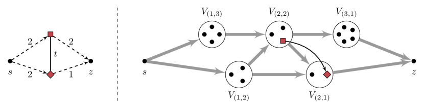
Figure 5: The left side depicts an excerpt of a reduced temporal graph with maximum time-edge label $\tau=4$. Dashed arcs labeled with a number $x$ indicate a shortest strict temporal path of length $x$. The right side depicts the directed path cover graph $D$ from $s$ to $z$ of the reduced temporal graph. A gray arc from vertex set $V_{(i,j)}$ to vertex set $V_{(i^{\prime},j^{\prime})}$ denotes that for two vertices $v\in V_{(i,j)}$ and $w\in V_{(i^{\prime},j^{\prime})}$ there can be an arc from $v$ to $w$ in $D$. Take as an example the square-shaped vertex in $V_{(2,2)}$ and the diamond-shaped vertex in $V_{(2,1)}$.

Definition 3.7 (Directed Path Cover Graph).

Let $\bm{G}=(V,\bm{E},\tau=4)$ be a reduced temporal graph with $s,z\in V$. The directed path cover graph from $s$ to $z$ of $\bm{G}$ is a directed graph $D=(V,\vec{E})$ such that $(v,w)\in\vec{E}$ if and only if (i) $v,w\in V$, (ii) $(\{v,w\},t)\in\bm{E}$for some $t\in[\tau]$, and (iii) $v\in V_{(i,j)}$and $w\in V_{(i^{\prime},j^{\prime})}$ such that $i<i^{\prime}$,  $v\in V_{(2,2)}$ and $w\in V_{(2,1)}$, $v=s$ and $w\in V_{(1,j)}$, or $w=z$ and $v\in V_{(i,1)}$ for some $i,j\in\{2,3\}$. Herein, a vertex $x\in V$ is in the set $V_{(i,j)}$ if the shortest strict temporal $(s,x)$-path is of length $i$ and the shortest strict temporal $(x,z)$-path is of length $j$.

Figure 5 depicts a generic directed path cover graph of a reduced temporal graph with $\tau=4$. Note that due to the definition of reduced temporal graphs, one can prove that the set $V_{(1,1)}$ is always empty, and hence not depicted in Figure 5. This is a crucial property that allows us to prove the following.

Lemma 3.8.

Let $\bm{G}=(V,\bm{E},\tau=4)$ be a reduced temporal graph with $s,z\in V$. Then the directed path cover graph $D$ from $s$ to $z$ of $\bm{G}$ can be computed in $\mathcal{O}(|\bm{E}|)$ time and $S\subseteq V\setminus\{s,z\}$ is a strict temporal $(s,z)$-separator in $\bm{G}$ if and only if $S$ is an $(s,z)$-separator in $D$.

We introduce some notation we will use in the following proof. The departure time (arrival time) of a temporal $(s,z)$-path $P=((e_{1},t_{1}),\dots,(e_{\ell},t_{\ell}))$ is $t_{1}$ ($t_{\ell}$), the traversal time of $P$ is $t_{\ell}-t_{1}$, and the length of $P$ is $\ell$.

Proof.

Let $\bm{G}=(V,\bm{E},\tau=4)$ be a reduced temporal graph with $s,z\in V$. In order to compute the directed path cover graph $D=(V,\vec{E})$ from $s$ to $z$ of $\bm{G}$, we need to know the shortest strict temporal $(s,v)$-path and the shortest strict temporal $(v,z)$-path in $\bm{G}$ for all $v\in V$. For $s$ this can be done in $\mathcal{O}(|\bm{E}|)$ time by Proposition 3.4. For $z$, consider the bijection $\lambda:[\tau]\to[\tau]$ with $\lambda(t)=\tau+1-t$ and the helping graph $\overleftarrow{\bm{G}}:=(V,\overleftarrow{\bm{E}},\tau)$ of $\bm{G}$ where $\overleftarrow{\bm{E}}:=\{(\{v,w\},\lambda(t))\mid(\{v,w\},t)\in\bm{E}\}$. Note that $\overleftarrow{\bm{G}}$ can be constructed in $O(|\bm{E}|)$ time. Moreover, it holds true that $P$ is a shortest strict temporal $(v,z)$-path in $\bm{G}$ if and only if $\overleftarrow{P}$ is a shortest strict temporal $(z,v)$-path in $\overleftarrow{\bm{G}}$, where $\overleftarrow{P}$ is $P$ where each temporal edge $(\{x,y\},t)$ in $P$ is replaced by $(\{x,y\},\lambda(t))$. If $P$ is not a shortest strict temporal $(v,z)$-path in $\bm{G}$, then there is a shorter strict temporal $(v,z)$-path $P^{\prime}$ in $\bm{G}$. Then $\overleftarrow{P^{\prime}}$ is a strict temporal $(z,v)$-path in $\overleftarrow{\bm{G}}$ shorter than $\overleftarrow{P}$. The other direction is proven analogously. It follows that computing the shortest strict temporal $(v,z)$-path in $\bm{G}$ for all $v\in V$ can be done in $\mathcal{O}(|\bm{E}|)$ time by employing Proposition 3.4 in $\overleftarrow{\bm{E}}$.

Now we iterate over the time-edge set $\bm{E}$ and check for each $(\{v,w\},t)$ whether there is an arc between $v$ and $w$ in $\vec{E}$. Hence, the directed path cover graph $D=(V,\vec{E})$ from $s$ to $z$ of $G$ can be computed in $\mathcal{O}(|\bm{E}|)$.

We say that a strict temporal $(s,z)$-path $P$ of length $n$ in $\bm{G}$ is chordless if $\bm{G}[V(P)]$ does not contain a strict temporal $(s,z)$-path $P^{\prime}$ of length $n-1$. If such a $P^{\prime}$ exists, we call $P^{\prime}$ a chord of $P$. Obviously, for a set $X$ of vertices, if $\bm{G}-X$ does not contain any chordless strict temporal $(s,z)$-path, then $\bm{G}-X$ does not contain any strict temporal $(s,z)$-path.

Now, we discuss the appearance of the directed path cover graph $D$. Assume towards a contradiction that there is a vertex $v\in V_{(1,1)}$. Since $\bm{G}$ is reduced, there is no strict temporal $(s,z)$-paths of length two. Thus, if there is a vertex $v\in V_{(1,1)}$, then there must be time-edges $(\{s,v\},t_{1})$ and $(\{v,z\},t_{2})$ such that $t_{2}\leq t_{1}$. We distinguish two cases.

Case 1:

Let $t_{2}\leq 2\leq t_{1}$. Since $\bm{G}$ is reduced, we know that there is a strict temporal $(s,z)$-path $P$ which contains $(\{v,z\},t_{2})$. The strict temporal $(s,z)$-path $P$ must be of length at least three, because $\bm{G}$ is reduced Observe that the length of a strict temporal $(s,z)$-path is a lower bound for the arrival time. Hence, the arrival time of $P$ is at least three. This is a contradiction because $(\{v,z\},t_{2})$ is the last time-edge of $P$ and, therefore, $t_{2}\leq 2$ is equal to the arrival time. Consequently, $v\notin V_{(1,1)}$.

Case 2:

Let $3\leq t_{2}\leq t_{1}$. Since $\bm{G}$ is reduced, we know that there is a strict temporal $(s,z)$-path $P$ which contains $(\{s,v\},t_{1})$. The strict temporal $(s,z)$-path $P$ must be of length at least three because $\bm{G}$ is reduced. Observe that $(\{s,v\},t_{1})$ is the first time-edge of $P$. Hence, the departure time of $P$ is at least three. Since, $P$ is of length at least three, the arrival time of $P$ is at least five. This is a contradiction because the maximum label is four. Consequently, $v\notin V_{(1,1)}$.

Observe that the sets $V_{(1,3)},V_{(2,2)},V_{(3,1)},V_{(1,2)},V_{(2,1)}$ are a partition of $V\setminus\{s,t\}$, because all strict temporal $(s,z)$-paths are of length at most four and $V_{(1,1)}=\emptyset$. In Figure 5, we can see the appearance of the directed path cover graph $D$ from $s$ to $z$ of $\bm{G}$.

We claim that for each chordless strict temporal $(s,z)$-path $P$ in $\bm{G}$, there is an $(s,z)$-path $P_{D}$ such that $V(P)=V(P_{D})$. Let $P$ be a chordless strict temporal $(s,z)$-path in $\bm{G}$. Since $\bm{G}$ is reduced, $P$ is of length three or four.

Case 1:

Let the length of $P$ be three and $V(P)=\{s,v_{1},v_{2},z\}$ such that $v_{1}$ is visited before $v_{2}$. Since there is no strict temporal $(s,z)$-path of length two, $P$ forces $v_{1}$ into $V_{(1,2)}$ and $v_{2}\in V_{(2,1)}$. It is easy to see that $v_{1}\in V_{(1,2)}$, just by the existence of $P$. For $v_{2}\in V_{(2,1)}$, we need that there is no strict temporal $(s,v_{2})$-path of length one.

Assume towards a contradiction that there would be a strict temporal $(s,v_{2})$-path of length one or in other words there is a time-edge $(\{s,v_{2}\},t)\in\bm{E}$. Then $v_{2}\in V_{(1,1)}$, which contradicts the fact that $V_{(1,1)}=\emptyset$, and hence $v_{2}\in V_{(2,1)}$.

From Definition 3.7, we know that there is an $(s,z)$-path $P_{D}$ such that $V(P)=V(P_{D})$.

Case 2:

Let the length of $P$ be four. Thus, it looks as follows.

$$P=((\{s,v_{1}\},1),(\{v_{1},v_{2}\},2),(\{v_{2},v_{3}\},3),(\{v_{3},z\},4)).$$

It immediately follows that the shortest strict temporal $(s,v_{1})$-path is of length one. Furthermore, the shortest strict temporal $(s,v_{2})$-path is of length two, otherwise $P$ would not be chordless.

Now, we claim that $v_{3}\in V_{(2,1)}\cup V_{(3,1)}$. Assume towards a contradiction that $v_{3}\notin V_{(2,1)}\cup V_{(3,1)}$. Observe that $v_{3}\notin V_{(2,2)}$ because $(\{v_{3},z\},4)$ is a shortest strict temporal $(v_{3},z)$-path of length one. Thus, there is a time-edge $(\{s,v_{3}\},t)\in\bm{E}$. This time-edge must be part of a strict temporal $(s,z)$-path, because $\bm{G}$ is reduced. Since $v_{3}\neq z$, we have $t\leq 3$. Note that $((\{s,v_{3}\},t\leq 3),(\{v_{3},z\},4))$ would be a strict temporal $(s,z)$-path of length two. Hence, $(\{s,v_{3}\},t)\notin\bm{E}$ and $v_{3}\in V_{(2,1)}\cup V_{(3,1)}$.

From Definition 3.7 we know that there is an $(s,z)$-path $P_{D}$ such that $V(P)=V(P_{D})$.

Let $S\subseteq(V\setminus\{s,z\})$ be an $(s,z)$-separator in $D$. Until now, we know that $S$ is also a strict temporal $(s,z)$-separator in $\bm{G}$, because for each chordless strict temporal $(s,z)$-path in $\bm{G}$ there is an $(s,z)$-path in $D$. Let $L\subseteq(V\setminus\{s,z\})$ be a strict temporal $(s,z)$-separator in $\bm{G}$. It remains to be shown that $L$ is an $(s,z)$-separator in $D$.

Assume towards a contradiction that $L$ is not an $(s,z)$-separator in $D$. Thus, there is an $(s,z)$-path $P_{D}$ in $D-L$. The length of $P_{D}$ is either three or four, see Figure 5.

Case 1:

Let the length of $P_{D}$ be three and $V(P_{D})=\{s,v_{1},v_{2},z\}$ such that $v_{1}$ is visited before $v_{2}$. Thus, $v_{1}\in V_{(1,2)}$ and $v_{2}\in V_{(2,1)}$, see Figure 5. From Definition 3.7, we know that there are time-edges $(\{s,v_{1}\},t_{1}),(\{v_{1},v_{2}\},t_{2}),(\{v_{2},z\},t_{3})\in\bm{E}$. Note that each time-edge in $\bm{G}$ must be part of a strict temporal $(s,z)$-path and that there are no strict temporal $(s,z)$-paths of length two. Hence, $t_{1}\in\{1,2\}$, $t_{2}\in\{2,3\}$, and $t_{3}\in\{3,4\}$. We distinguish the cases $t_{2}=2$ and $t_{2}=3$.

Case 1.1:

Let $t_{2}=2$. The time-edge $(\{v_{1},v_{2}\},t_{2}=2)$ must be part of a strict temporal $(s,z)$-path, and therefore we have either $(\{s,v_{2}\},1)\in\bm{E}$ or $(\{s,v_{1}\},1)\in\bm{E}$. Time-edge $(\{s,v_{2}\},1)$ cannot exist since $v_{2}\in V_{(2,1)}$. Hence, $(\{s,v_{1}\},1)\in\bm{E}$, $t_{1}=1$, and $((\{s,v_{1}\},t_{1}),(\{v_{1},v_{2}\},t_{2}),(\{v_{2},z\},t_{3}))$ is a strict temporal $(s,z)$-path in $\bm{G}$. Moreover, $\{v_{1},v_{2}\}\cap L\neq\emptyset$. This contradicts the fact that $L$ is strict temporal $(s,z)$-separator in $\bm{G}$.

Case 1.2:

Let $t_{2}=3$. There is a strict temporal $(s,z)$-path which contains the time-edge $(\{v_{1},v_{2}\},t_{2}=3)$. Since $t_{3}\geq 3$, there is either a $(\{v_{1},z\},4)\in\bm{E}$ or $(\{v_{2},z\},4)\in\bm{E}$. The time-edge $(\{v_{1},z\},4)$ cannot exist because $v_{1}\in V_{(1,2)}$. Hence $(\{v_{2},z\},4)\in\bm{E}$, $t_{3}=4$, and $((\{s,v_{1}\},t_{1}),(\{v_{1},v_{2}\},t_{2}),(\{v_{2},z\},t_{3}))$ is a strict temporal $(s,z)$-path in $\bm{G}$. Moreover, $\{v_{1},v_{2}\}\cap L\neq\emptyset$. This contradicts the fact that $L$ is strict temporal $(s,z)$-separator in $\bm{G}$.

Case 2:

Let the length of $P_{D}$ be four, and $V(P_{D})=\{s,v_{1},v_{2},v_{3},z\}$ such that $v_{1}$ is visited before $v_{2}$ and $v_{2}$ is visited before $v_{3}$. Considering Figure 5, one can observe that $v_{1}\in V_{(1,3)}\cup V_{(1,2)}$ and $v_{2}\in V_{(2,2)}$. From Definition 3.7, we know that there are time-edges $(\{s,v_{1}\},t_{1}),(\{v_{1},v_{2}\},t_{2}),$ $(\{v_{2},v_{3}\},t_{3}),(\{v_{3},z\},t_{4})\in\bm{E}$. There is a strict temporal $(s,z)$-path $P$ containing $(\{v_{1},v_{2}\},t_{2})$ because $\bm{G}$ is reduced. Since $v_{2}\in V_{(2,2)}$, we know that $P$ is of length four.

Now assume towards a contradiction that $P$ visits $v_{2}$ before $v_{1}$. Hence, $(\{v_{1},v_{2}\},t_{2})$ is the third time-edge in $P$. The first two time-edges of $P$ are a strict temporal $(s,v_{2})$-path of length two and arrival time at least two. Thus, $t_{2}\geq 3$. Observe that there is no strict temporal $(v_{1},z)$-path of length one and hence there is no time-edge $(\{v_{1},z\},4)$, because $v_{1}\in V_{(1,2)}\cup V_{(1,3)}$. This contradicts $P$ visiting $v_{2}$ before $v_{1}$. Consequently, the strict temporal $(s,z)$-path $P$ visits $v_{1}$ before $v_{2}$ and  $(\{v_{1},v_{2}\},t_{2})$ is the second time-edge in $P$. Hence, $t_{2}=2$ and there is a time-edge $(\{s,v_{1}\},1)$ in $P$. This implies $t_{1}=1$.

The vertex $v_{3}\in V_{(2,1)}\cup V_{(3,1)}$, see Figure 5. There is a strict temporal $(s,z)$-path which contains $(\{v_{2},v_{3}\},t_{3})$, because $\bm{G}$ is reduced. Since $v_{3}\in V_{(2,1)}\cup V_{(3,1)}$ and $v_{2}\in V_{(2,2)}$, all strict temporal $(s,v_{2})$-paths and strict temporal $(s,v_{3})$-paths have length at least two and thus also arrival time at least two. Hence, $t_{3}\geq 3$. Because $v_{2}\neq z\neq v_{3}$ and there is a strict temporal $(s,z)$-path which contains $(\{v_{2},v_{3}\},t_{3})$, we have $t_{3}<4\Rightarrow t_{3}=3$ and there is either a time-edge $(\{v_{2},z\},4)\in\bm{E}$ or $(\{v_{3},z\},4)\in\bm{E}$. The time-edge $(\{v_{2},z\},4)$ cannot exist, otherwise there would be a strict temporal $(v_{2},z)$-path of length one, but $v_{2}\in V_{(2,2)}$. This implies that $(\{v_{3},z\},4)\in\bm{E}$ and $t_{4}=4$. Hence, the time-edge sequence $((\{s,v_{1}\},t_{1}),(\{v_{1},v_{2}\},t_{2}),$ $(\{v_{2},v_{3}\},t_{3}),(\{v_{3},z\},t_{4}))$ forms a strict temporal $(s,z)$-path and $\{v_{1},v_{2},v_{3}\}\cap L\neq\emptyset$. This contradicts the fact that $L$ is strict temporal $(s,z)$-separator in $\bm{G}$.

In summary, $P_{D}$ cannot exist in $D-L$. Consequently, $L$ is an $(s,z)$-separator in $D$. ∎

Figure 6 shows that if $\tau=5$, then we can construct a reduced temporal graph where the set $V_{(1,1)}$ is not empty. This indicates why our algorithm fails for $\tau=5$.

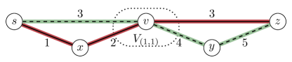
Figure 6: A reduced temporal graph with maximum label $\tau=5$ where the vertex set $V_{(1,1)}$ of the directed path cover graph is not empty. The solid (red) and dashed (green) edges are strict temporal paths and show that edges $(\{s,v\},3)$ and $(\{v,z\},3)$ are not removed when the graph is reduced. Furthermore, $v$ is not removed since $((\{s,v\},3),(\{v,z\},3))$ is not a strict temporal path.

Finally, with Lemmata 3.5 and 3.8 we can prove Theorem 3.6.

Proof of Theorem 3.6.

Let $\mathcal{I}:=(\bm{G}=(V,\bm{E},\tau=4),s,z,k)$ be an instance of Strict Temporal $(s,z)$-Separation. First, apply Lemma 3.5 in $\mathcal{O}(k\cdot|\bm{E}|)$ time to either decide $\mathcal{I}$ or to obtain an instance $\mathcal{I}^{\prime}=(\bm{G}^{\prime}=(V^{\prime},\bm{E}^{\prime},\tau),s,z,k^{\prime})$ of Strict Temporal $(s,z)$-Separation. In the second case, compute the directed path cover graph $D$ of $\bm{G}^{\prime}$ from $s$ to $z$ in $\mathcal{O}(|\bm{E}^{\prime}|)$ time (by Lemma 3.8). Next, check whether $D$ has an $(s,z)$-separator of size at most $k^{\prime}$ in $\mathcal{O}(k^{\prime}\cdot|\bm{E}^{\prime}|)$ time by a folklore result [21]. By Lemma 3.8, $D$ has an $(s,z)$-separator of size $k^{\prime}$ if and only if $\bm{G}^{\prime}$ has a strict temporal $(s,z)$-separator of size $k^{\prime}$. Since by Lemma 3.5 we have that $\bm{G}^{\prime}$ is reduced, $|V^{\prime}|\leq|V|$, $|\bm{E}^{\prime}|\leq|\bm{E}|$, and $k^{\prime}\leq k$, the overall running time is $\mathcal{O}(k\cdot|\bm{E}|)$. ∎

4 On Temporal Graphs with Planar Underlying Graph

In this section, we study our problems on planar temporal graphs, that is, temporal graphs that have a planar underlying graph. We show that both Temporal $(s,z)$-Separation and Strict Temporal $(s,z)$-Separation remain NP-complete on planar temporal graphs. On the positive side, we show that on planar temporal graphs with a constant number of layers, Strict Temporal $(s,z)$-Separation can be solved in $\mathcal{O}(|\bm{E}|\cdot\log|\bm{E}|)$ time.

In order to prove our hardness results, we first prove NP-hardness for Length-Bounded $(s,z)$-Separation on planar graphs—a result which we consider to be of independent interest; note that NP-completeness on planar graphs was only known for the edge-deletion variant of Length-Bounded $(s,z)$-Separation on undirected graphs [19] and weighted directed graphs [35].

Theorem 4.1.

Length-Bounded $(s,z)$-Separation on planar graphs is NP-hard.

Proof.

We give a many-one reduction from the NP-complete [19] edge-weighted variant of Length-Bounded $(s,z)$-Cut, referred to as Planar Length-Bounded $(s,z)$-Cut, where the input graph $G=(V,E)$ is planar, has edge costs $c:E\to\{1,k+1\}$, has maximum degree $\Delta=6$, the degree of $s$ and $z$ is three, and $s$ and $z$ are incident to the outer face. Since the maximum degree is constant, one can replace a vertex with a planar grid-like gadget.

Let $\mathcal{I}:=(G=(V,E,c),s,z,\ell,k)$ be an instance of Planar Length-Bounded $(s,z)$-Cut, and we assume $k$ to be even. We construct an instance $\mathcal{I}^{\prime}:=(G^{\prime},s^{\prime},z^{\prime},\ell^{\prime},k)$ of Length-Bounded $(s,z)$-Separation as follows (refer to Figure 7 for an illustration).

Construction. For each vertex $v\in V$, we introduce a vertex-gadget $G_{v}$ which is a grid of size $(2k+2)\times(2k+2)$, that is, a graph with vertex set $~{}\{u^{v}_{i,j}\mid i,j\in[2k+2]\}$ and edge set $\{\{u^{v}_{i,j},u^{v}_{i^{\prime},j^{\prime}}\}\mid|i-i^{\prime}|+|j-j^{\prime}|=1\}$. There are six pairwise disjoint subsets $C_{v}^{1},\dots,C_{v}^{6}\subseteq V(G_{v})$ of size $k+1$ that we refer to as connector sets. As we fix an orientation of $G_{v}$ such that $u^{v}_{1,1}$ is in the top-left, there are two connector sets on the top of $G_{v}$, two on the bottom of $G_{v}$, one on the left of $G_{v}$, and one on the right of $G_{v}$. Formally, $C_{v}^{1}=\{u^{v}_{1,k+2},\ldots,u^{v}_{1,2k+2}\}$, $C_{v}^{2}=\{u^{v}_{k/2,2k+2},\ldots,u^{v}_{3k/2,2k+2}\}$, $C_{v}^{3}=\{u^{v}_{2k+2,k+2},\ldots,u^{v}_{2k+2,2k+2}\}$, $C_{v}^{4}=\{u^{v}_{2k+2,1},\ldots,u^{v}_{2k+2,k+1}\}$, $C_{v}^{5}=\{u^{v}_{k/2,1},\ldots,u^{v}_{3k/2,1}\}$, and $C_{v}^{6}=\{u^{v}_{1,1},\ldots,u^{v}_{1,k+1}\}$.

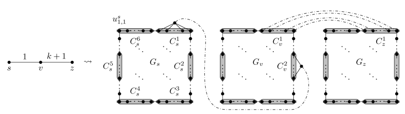
Figure 7: A simple planar graph $G$ (left) with edge costs (above edges) and the obtained graph $G^{\prime}$ in the reduction from Theorem 4.1. The connector sets are highlighted in gray. The edge-gadgets are indicated by dash-dotted lines.

Note that all $(x,y)$-paths are of length at most $k^{\prime}:=(2k+2)^{2}-1$, for all $x,y\in V(G_{v})$, because there are only $(2k+2)^{2}$ vertices in $V(G_{v})$.

Let $\phi(G)$ be a plane embedding of $G$. We say that an edge $e$ incident with vertex $v\in V$ is at position $i$ on $v$ if $e$ is the $i$th edge incident with $v$ when counted clockwise with respect to $\phi(G)$. For each edge $e=\{v,w\}$, we introduce an edge-gadget $G_{e}$ that differs on the weight of $e$, as follows. Let $e$ be at position $i\in\{1,\dots,6\}$ on $v$ and at position $j\in\{1,\dots,6\}$ on $w$. If $c(e)=1$, then $G_{e}$ is constructed as follows. Add a path consisting of $(\ell+1)\cdot k^{\prime}-1$ vertices and connect one endpoint with each vertex in $C_{v}^{i}$ by an edge and connect the other endpoint with each vertex in $C_{w}^{j}$ by an edge. If $c(e)=k+1$, then $G_{e}$ is constructed as follows. We introduce a planar matching between the vertices in $C_{v}^{i}$ and $C_{w}^{j}$. That is, for instance, we connect vertex $u^{v}_{1,k+2+p}$ with vertex $u^{w}_{1,2k+2-p}$ for each $p\in\{0,\ldots,k\}$, if $i=j=1$, or we connect vertex $u^{v}_{1,1+p}$ with vertex $u^{w}_{2k+2,3k/2-p}$ for each $p\in\{0,\ldots,k\}$, if $i=6$ and $j=2$ (we omit the remaining cases). Then, replace each edge by a path of length at least $(\ell+1)\cdot k^{\prime}+1$ where its endpoints are identified with the endpoints of the replaced edge. Hence, a path between two vertex-gadgets has length at least $(\ell+1)\cdot k^{\prime}+1$.

Next, we choose connector sets $C_{s}^{i^{\prime}}$ and $C_{z}^{j^{\prime}}$ such that no vertex $v\in C_{s}^{i^{\prime}}\cup C_{z}^{j^{\prime}}$ is adjacent to a vertex from an edge-gadget. Such $i^{\prime}$ and $j^{\prime}$ always exist because the degrees of $s$ and $z$ are both three. Now, we add two special vertices $s^{\prime}$ and $z^{\prime}$ and edges between $s^{\prime}$ and each vertex in $C_{s}^{i^{\prime}}$, as well as between $z^{\prime}$ and each vertex in $C_{z}^{j^{\prime}}$.

Finally, we set $\ell^{\prime}:=2+(\ell+1)\cdot k^{\prime}+\ell\left((\ell+1)\cdot k^{\prime}+1\right).$ Note that $G^{\prime}$ can be computed in polynomial time. Moreover, one can observe that $G^{\prime}$ is planar by obtaining an embedding from $\phi$. This concludes the description of the construction.

Correctness. We claim that $\mathcal{I}$ is a yes-instance if and only if $\mathcal{I}^{\prime}$ is a yes-instance.

$\Rightarrow$: Let $\mathcal{I}$ be a yes-instance. Thus, there is a solution $C\subset E$ with $c(C)\leq k$ such that there is no $(s,z)$-path of length at most $\ell$ in $G-C$. We construct a set $S\subset V(G^{\prime})$ of size at most $k$ by taking for each $\{v,w\}\in C$ one arbitrary vertex from the edge-gadget $G_{\{v,w\}}$ into $S$. Note that since $c(C)\leq k$, each edge in $C$ is of cost one.

Assume towards a contradiction that there is a shortest $(s^{\prime},z^{\prime})$-path $P^{\prime}$ of length at most $\ell^{\prime}$ in $G^{\prime}-S$. Since a path between two vertex-gadgets has length at least $(\ell+1)\cdot k^{\prime}+1$, we know that $P^{\prime}$ goes through at most $\ell$ edge-gadgets. Otherwise $P^{\prime}$ would be of length at least $2+(\ell+1)\cdot\left[(\ell+1)\cdot k^{\prime}+1\right]=2+(\ell+1)\cdot k^{\prime}+\ell\cdot\left[(\ell+1)\cdot k^{\prime}+1\right]+1=\ell^{\prime}+1.$ Now, we reconstruct an $(s,z)$-path $P$ in $G$ corresponding to $P^{\prime}$ by taking an edge $e\in E$ into $P$ if $P^{\prime}$ goes through the edge-gadget $G_{e}$. Hence, the length of $P$ is at most $\ell$. This contradicts that there is no $(s,z)$-path of length at most $\ell$ in $G-C$. Consequently, there is no $(s^{\prime},z^{\prime})$-path of length at most $\ell^{\prime}$ in $G^{\prime}-S$ and $\mathcal{I}^{\prime}$ is a yes-instance.

$\Leftarrow$: Let $\mathcal{I}^{\prime}$ be a yes-instance. Thus, there is a solution $S\subseteq V(G^{\prime})$ of minimum size (at most $k$) such that there is no $(s^{\prime},z^{\prime})$-path of length at most $\ell^{\prime}$ in $G^{\prime}-S$. Since $S$ is of minimum size, it follows from the following claim that $V(G_{v})\cap S=\emptyset$ for all $v\in V$.

Claim 4.2.

Let $G_{v}$ be a vertex-gadget and $i,j\in\{1,\dots,6\}$ with $i\neq j$. Then, for each vertex set $S\subseteq V(G_{v})$ of size at most $k$ it holds that there are $v_{1}\in C_{v}^{i}\setminus S$ and $v_{2}\in C_{v}^{j}\setminus S$ such that there is a $(v_{1},v_{2})$-path of length at most $k^{\prime}$ in $G_{v}-S$.

Proof of Claim 4.2.

Let $C_{v}^{i},C_{v}^{j}$ two connector sets of a vertex-gadget $G_{v}$, where $i,j\in\{1,\dots,6\}$ and $i\not=j$. We add vertices $a$ and $b$ and edges $\{a,a^{\prime}\}$ and $\{b,b^{\prime}\}$ to $G_{v}$, where $a^{\prime}\in C_{v}^{i}$ and $b^{\prime}\in C_{v}^{j}$. There are $6\choose 2$ different cases in which $i\not=j$. It is not difficult to see that in each case there are $k+1$ vertex-disjoint $(a,b)$-paths. The claim then follows by Menger’s Theorem [31]. ∎

Note that by minimality of $S$, it holds that $V(G_{e})\cap S=\emptyset$ for all $e\in E$ with $c(e)=k+1$. We construct an edge set $C\subseteq E$ of cost at most $k$ by taking $\{v,w\}\in E$ into $C$ if there is a $y\in V(G_{\{v,w\}})\cap S$.

Assume towards a contradiction that there is a shortest $(s,z)$-path $P$ of length at most $\ell$ in $G-C$. We reconstruct an $(s^{\prime},z^{\prime})$-path $P^{\prime}$ in $G^{\prime}$ which corresponds to $P$ as follows. First, we take an edge $\{s^{\prime},v\}\in E(G^{\prime})$ such that $v\in C_{s}^{i^{\prime}}\setminus S$. Such a $v$ always exists, because $|C_{s}^{i^{\prime}}|=k+1$ and $|S|\leq k$. Let $\{s,w\}\in E$ be the first edge of $P$ and at position $i$ on $w$. Then we add a $(v,v^{\prime})$-path $P_{s}$ in $G_{s}-S$, such that $v^{\prime}\in C_{s}^{i}\setminus S$. Due to Claim 4.2, such a $(v,v^{\prime})$-path $P_{s}$ always exists in $G_{s}-S$ and is of length at most $k^{\prime}$.

We take an edge-gadget $G_{e}$ into $P^{\prime}$ if $e$ is in $P$. Recall, that an edge-gadget is a path of length $(\ell+1)\cdot k^{\prime}+1$. Due to Claim 4.2, we can connect the edge-gadgets $G_{\{v_{1},v_{2}\}},G_{\{v_{2},v_{3}\}}$ of two consecutive edges $\{v_{1},v_{2}\},\{v_{2},v_{3}\}$ in $P$ by a path of length at most $k^{\prime}$ in $G_{v_{2}}$. Let $\{v_{p},z\}$ be the last edge in $P$, be at position $j$ on $z$, $v\in C_{z}^{j}$, and $v^{\prime}\in C_{z}^{j^{\prime}}$. We add a $(v,v^{\prime})$-path of length $k^{\prime}$ in $G_{z}-S$ (Claim 4.2). Note that $P^{\prime}$ visits at most $\ell+1$ vertex-gadgets and $\ell$ edge-gadgets. The length of $P^{\prime}$ is at most $2+(\ell+1)\cdot k^{\prime}+\ell\left[(\ell+1)\cdot k^{\prime}+1\right]=\ell.$ This contradicts that $S$ forms a solution for $\mathcal{I}^{\prime}$. It follows that there is no $(s,z)$-path of length at most $\ell$ in $G-C$ and $\mathcal{I}$ is a yes-instance. ∎

From the proofs of Theorems 3.1 and 2.1 (planarity-preserving reductions for the underlying graph), together with Theorem 4.1 we get the following:

Corollary 4.3.

Both Temporal $(s,z)$-Separation and Strict Temporal $(s,z)$-Separation on planar temporal graphs are NP-complete.

In contrast to the case of general temporal graphs, Strict Temporal $(s,z)$-Separation on planar temporal graphs is efficiently solvable if the maximum label $\tau$ is any constant. To this end, we introduce monadic second-order (MSO) logic and the optimization variant of Courcelle’s Theorem [5, 13].

Monadic second-order (MSO) logic consists of a countably infinite set of (individual) variables, unary relation variables, and a vocabulary. A formula in monadic second-order logic on graphs is constructed from the vertex variables, edge variables, an incidence relation between edge and vertex variables ${\rm inc}(e,x)$, the relations $=,\land,\lor,\neg$, and the quantifiers $\forall$ and $\exists$. We will make use of many folklore shortcuts, for example: $\not=$, $\subseteq$ , $v\in V$ to check whether $v$ is a vertex variable, and $e\in E$ to check whether $e$ is an edge variable. The treewidth $\operatorname{tw}(G)$ of a graph $G$ measures how tree-like a graph is. In this paper we are using the following theorem and the treewidth of a graph as a black box. For formal definitions of treewidth and MSO, refer to Courcelle and Engelfriet [13].

Theorem 4.4 (Arnborg et al. [5], Courcelle and Engelfriet [13]).

There exists an algorithm that, given

1. an MSO formula $\rho$ with free monadic variables $X_{1},\dots,X_{r}$,

2. an affine function $\alpha(x_{1},\dots,x_{r})$, and

3. a graph $G$,

finds the minimum (maximum) of $\alpha(|X_{1}|,\dots,|X_{r}|)$ over evaluations of $X_{1},\dots,X_{r}$ for which formula $\rho$ is satisfied on $G$. The running time is $f(|\rho|,\operatorname{tw}(G))\cdot|G|$, where $|\rho|$ is the length of $\rho$, and $\operatorname{tw}(G)$ is the treewidth of $G$.

We employ Theorem 4.4 to solve Strict Temporal $(s,z)$-Separation on planar temporal graphs.

Proposition 4.5.

Strict Temporal $(s,z)$-Separation on planar temporal graphs can be solved in $\mathcal{O}(|\bm{E}|\cdot\log|\bm{E}|)$ time, if the maximum label $\tau$ is constant.

Proof.

Let $\mathcal{I}=(\bm{G}=(V,\bm{E},\tau),s,z,k)$ be an instance of Strict Temporal $(s,z)$-Separation, where the underlying graph of $\bm{G}$ is planar.

We define the optimization variant of Strict Temporal $(s,z)$-Separation in monadic second order logic (MSO) and show that it is sufficient to solve the Strict Temporal $(s,z)$-Separation on a temporal graph where we can upper-bound the treewidth of the underlying graph by a function only depending on $\tau$.

We define the edge-labeled graph $L(\bm{G})$ to be the underlying graph ${G}_{\downarrow}$ of $\bm{G}$ with the edge-labeling $\omega:E({G}_{\downarrow})\rightarrow[2^{\tau}-1]$ with $\omega(\{v,w\})=\sum_{i=1}^{\tau}\mathds{1}_{\{v,w\}\in E_{i}}\cdot 2^{i-1}$, where $\mathds{1}_{\{v,w\}\in E_{i}}=1$ if and only if $(\{v,w\},i)\in\bm{E}$, and $0$ otherwise. Observe that in binary representation, the $i$-th bit of $\omega(\{v,w\})$ is one if and only if $\{v,w\}$ exists at time point $i$. To compute $L(\bm{G})$ we first iterate over the time-edge set $\bm{E}$ and add an edge $\{v,w\}$ to the edge set $E$ of the underlying graph $L(\bm{G})$ whenever we find a time-edge $\big{(}\{v,w\},t\big{)}\in\bm{E}$. Furthermore, we associate with each edge in $E$ an integer $\omega_{\{v,w\}}$ which is initially zero, and gets an increment of $2^{t-1}$ for each time-edge $\big{(}\{v,w\},t\big{)}\in\bm{E}$. With the appropriate data structure, this can be done in $\mathcal{O}(|\bm{E}|\cdot\log|\bm{E}|)$ time. Observe, that in the end $\omega_{\{v,w\}}=\omega(\{v,w\})$. Finally, we copy the vertex set of $\bm{G}$, and hence compute $L(\bm{G})$ in $\mathcal{O}(|V|+|\bm{E}|\cdot\log|\bm{E}|)=\mathcal{O}(|\bm{E}|\cdot\log|\bm{E}|)$ time.

Arnborg et al. [5] showed that it is possible to apply Theorem 4.4 to graphs in which edges have labels from a fixed finite set, either by augmenting the graph logic to incorporate predicates describing the labels, or by representing the labels by unquantified edge set variables. Since Theorem 4.4 gives a linear-time algorithm with respect to the input size, we can conclude that if the size of that label set depends on $\tau$, then Theorem 4.4 still gives a linear-time algorithm for arbitrary but fixed $\tau$, the size of the MSO formula, and the treewidth.

We will define the optimization variant of Strict Temporal $(s,z)$-Separation in MSO on $L(\bm{G})$. First, the MSO formula ${\rm layer}(e,t):=~{}\bigvee_{i=1}^{\tau}\bigvee_{j\in\sigma(i,2^{\tau}-1)}\big{(}t=i~{}\land\omega(e)=j\big{)}$ checks whether an edge $e$ is present in the layer $t$, where $\sigma(i,j):=\{x\in[j]\,|\,\mathopen{}i\text{-th bit of }x\text{ is 1}\}$. Note that the length of ${\rm layer}(e,t)$ is upper-bounded by a some function in $2^{\mathcal{O}(\tau)}$. Second, we can write an MSO formula ${\rm tempadj}(v,w,t):=~{}\exists_{e\in E}\big{(}{\rm inc}(e,v)\land{\rm inc}(e,w)\land{\rm layer}(e,t)\big{)}$ to determine whether two vertices $v$ and $w$ are adjacent at time point $t$. Since the length of ${\rm layer}(e,t)$ is upper-bounded by some function in $2^{\mathcal{O}(\tau)}$, the length of ${\rm tempadj}(v,w,t)$ is upper-bounded by some function in $2^{\mathcal{O}(\tau)}$ as well. Third, there is an MSO formula

$${\rm path}(S):=\exists_{x_{1},\dots,x_{\tau+1}\in V\setminus S}\Big{(}x_{1}=s\land x_{\tau+1}=z\land\bigwedge_{i=1}^{\tau}\big{(}x_{i}=x_{i+1}\lor{\rm tempadj}(x_{i},x_{i+1},i)\big{)}\Big{)}$$

to check whether there is a strict temporal $(s,z)$-path which does not visit any vertex in $S$. Observe, that the length of ${\rm path}(S)$ is upper-bounded by some function in $2^{\mathcal{O}(\tau)}$. Finally, with Theorem 4.4 we can solve the optimization variant of Strict Temporal $(s,z)$-Separation by the formula $\phi(S):=S\subseteq(V\setminus\{s,z\})\land\neg{\rm path}(S)$ and the affine function $\alpha(x)=x$ in $f(\tau,\operatorname{tw}({G}_{\downarrow}))\cdot|V|$ time, where $f$ is some computable function. This gives us an overall running time of $\mathcal{O}(f(\tau,\operatorname{tw}({G}_{\downarrow}))\cdot|\bm{E}|\cdot\log|\bm{E}|)$ to decide $\mathcal{I}$ for Strict Temporal $(s,z)$-Separation.

Note that every strict temporal $(s,z)$-path in $\bm{G}$ and its induced $(s,z)$-path in ${G}_{\downarrow}$ have length at most $\tau$. Hence, we can remove all vertices from ${G}_{\downarrow}$ which are not reachable from $s$ by a path of length at most $\tau$. We can find the set of vertices $N$ which is reachable by a path of length $\tau$ by a breadth first search from $s$ in linear time. Therefore, it is sufficient to solve the Strict Temporal $(s,z)$-Separation on $\bm{G}[N\cup\{s\}]$. Observe, that $L(\bm{G}[N\cup\{s\}])$ has diameter at most $2\cdot\tau$ and is planar. The treewidth of a planar graph is at most three times the diameter (see Flum and Grohe [18]). Thus, (the optimization variant of) Strict Temporal $(s,z)$-Separation can be solved in $f^{\prime}(\tau)\cdot|\bm{E}|\cdot\log|\bm{E}|$ time, where $f^{\prime}$ is a computable function. For any constant $\tau$, this yields a running time of $\mathcal{O}(|\bm{E}|\cdot\log|\bm{E}|)$. ∎

5 On Temporal Graphs with Small Temporal Cores

In this section, we investigate the complexity of deciding (Strict) Temporal $(s,z)$-Separation on temporal graphs where the number of vertices whose incident edges change over time is small. We call the set of such vertices the temporal core of the temporal graph.

Definition 5.1 (Temporal core).

For a temporal graph $\bm{G}=(V,\bm{E},\tau)$, the vertex set $W=\{v\in V\mid\exists\{v,w\}\in(\bigcup_{i=1}^{\tau}E_{i})\setminus(\bigcap_{i=1}^{\tau}E_{i})\}\subseteq V$ is called the temporal core.

A temporal graph is often composed of a public transport system and an ordinary street network. Here, the temporal core consists of vertices involved in the public transport system.

For Strict Temporal $(s,z)$-Separation, we can observe that the hardness reduction described in the proof of Theorem 3.1 produces an instance with an empty temporal core. In stark contrast, we show that Temporal $(s,z)$-Separation is fixed-parameter tractable when parameterized by the size of the temporal core. We reduce an instance to Node Multiway Cut (NWC) in such a way that we can use an above lower bound FPT-algorithm due to Cygan et al. [14] for NWC as a subprocedure in our algorithm for Temporal $(s,z)$-Separation. Note that the above lower bound parameterization is crucial to obtain the desired FPT-running time bound. Recall the definition of NWC:

Node Multiway Cut (NWC)

Input:	An undirected graph $G=(V,E)$, a set of terminals $T\subseteq V$, and an integer $k$.
Question:	Is there a set $S\subseteq(V\setminus T)$ of size at most $k$ such there is no $(t_{1},t_{2})$-path for every distinct $t_{1},t_{2}\in T$?

We remark that Cygan et al.’s algorithm can be modified to obtain a solution $S$. Formally, we show the following.

Theorem 5.2.

Temporal $(s,z)$-Separation can be solved in $2^{|W|\cdot(\log|W|+2)}\cdot|V|^{\mathcal{O}(1)}+\mathcal{O}(|\bm{E}|\log|\bm{E}|)$ time, where $W$ denotes the temporal core of the input graph.

Proof.

Let instance $\mathcal{I}=(\bm{G}=(V,\bm{E},\tau),s,z,k)$ of Temporal $(s,z)$-Separation with temporal core $W\subseteq V$ be given. Without loss of generality, we can assume that $s,z\in W$, as otherwise we add two vertices one being incident only with $s$ and the other being incident only with $z$, both only in layer one. Furthermore, we need the notion of a maximal static subgraph $\widehat{G}$ of a temporal graph $\bm{G}=(V,\bm{E})$: It contains all edges that appear in every layer, more specifically $\widehat{G}=(V,\widehat{E})$ with $\widehat{E}=\bigcap_{i\in[\tau]}E_{i}$. Our algorithm works as follows.

1. Guess a set $S_{W}\subseteq(W\setminus\{s,z\})$ of size at most $k$.

2. Guess a number $r$ and a partition $\{W_{1},\dots,W_{r}\}$ of $W\setminus S_{W}$ such that $s$ and $z$ are not in the same $W_{i}$, for some $i\in[r]$.

3. Construct the graph $G^{\prime}$ by copying $\widehat{G}-W$ and adding a vertex $w_{i}$ for each part $W_{i}$. Add edge sets $\{\{v,w_{i}\}\mid v\in N_{\widehat{G}}(W_{i})\setminus W\}$ for all $i\in[r]$ and for all $i,j\in[r]$ add an edge $\{w_{i},w_{j}\}$ if $N_{\widehat{G}}(W_{i})\cap W_{j}\neq\emptyset$.

4. Solve the NWC instance $\mathcal{I}^{\prime}=(G^{\prime},\{w_{1},\dots,w_{r}\},k-|S_{W}|)$.

5. If a solution $S^{\prime}$ is found for $\mathcal{I}^{\prime}$ and $S^{\prime}\cup S_{W}$ is a solution for $\mathcal{I}$, then output yes.

6. If all possible guesses in (1) and (2) are considered without finding a solution for $\mathcal{I}$, then output no.

See Figure 8 for a visualization of the constructed graph $G^{\prime}$.

Figure 8: Illustration of the idea behind the proof of Theorem 5.2. Left-hand side: Sketch of a temporal graph $\bm{G}$ (enclosed by the ellipse) with temporal $(s,z)$ separator $S$ (red hatched) and induced partition $\{S_{W},W_{1},W_{2},W_{3}\}$ of the temporal core $W$, where $S_{W}=W\cap S$. The outer rings of $W_{1},W_{2},W_{3}$ contain the open neighborhood of the sets. Right-hand side: Sketch of the constructed graph $G^{\prime}$ (enclosed by the ellipse). The partition $\{S_{W},W_{1},W_{2},W_{3}\}$ is guessed in steps (1) and (2). The vertices $w_{1},w_{2},w_{3}$ with edges to the neighborhood of $W_{1},W_{2},W_{3}$, respectively, are created in step (3).

Since we do a sanity check in step (5) it suffices to show that if $\bm{G}$ has a temporal $(s,z)$-separator of size at most $k$, then there is a partition $\{S_{W},W_{1},\dots,W_{r}\}$ of $W$ where $s$ and $z$ are in different parts such that (i) the NWC instance $\mathcal{I}^{\prime}$ has a solution of size at most $k-|S_{W}|$, and (ii) if $S^{\prime}$ is a solution to $\mathcal{I}^{\prime}$, then $S_{W}\cup S^{\prime}$ is a temporal $(s,z)$-separator in $\bm{G}$.

Let $S$ be a temporal $(s,z)$-separator of size at most $k$ in $\bm{G}$. First, we set $S_{W}=S\cap W$. Let $C_{1},\dots,C_{r}$ be the connected components of $\widehat{G}-S$ with $C_{i}\cap W\neq\emptyset$ for all $i\in[r]$. Now we construct a partition $\{S_{W},W_{1},\dots,W_{r}\}$ of $W$ such that $W_{i}=W\cap C_{i}$ for all $i\in[r]$. It is easy to see that $s$ and $z$ are in different parts of this partition. Observe that for $i,j\in[r]$ with $i\neq j$ the vertices $v\in W_{i}$ and $u\in W_{j}$ are in different connected components of $\widehat{G}-S$. Hence, $w_{1},\dots,w_{r}$ are in different connected components of $G^{\prime}-(S\setminus S_{W})$. Thus $S\setminus S_{W}$ is a solution of size at most $k-|S_{W}|$ of the NWC instance $\mathcal{I}^{\prime}=(G^{\prime},\{w_{1},\dots,w_{r}\},k-|S_{W}|)$, proving (i).

For the correctness, it remains to prove (ii). Let $S^{\prime}$ be a solution of size at most $k-|S_{W}|$ of the NWC instance $\mathcal{I}^{\prime}$. We need to prove that $S^{\prime}\cup S_{W}$ forms a temporal $(s,z)$-separator in $\bm{G}$. Clearly, if $S^{\prime}=S\setminus S_{W}$, we are done by the arguments before. Thus, assume $S^{\prime}\neq S\setminus S_{W}$. Since $S^{\prime}$ is a solution to $\mathcal{I}^{\prime}$, we know that $w_{1},\dots,w_{r}$ are in different connected components of $G^{\prime}-S^{\prime}$. Hence, for $i,j\in[r]$ with $i\neq j$ the vertices $v\in W_{i}$, $u\in W_{j}$ are in different connected components of $\widehat{G}-(S^{\prime}\cup S_{W})$.

Now assume towards a contradiction that there is a temporal $(s,z)$-path $P$ in $\bm{G}-(S^{\prime}\cup S_{W})$. Observe that $\{s,z\}\subseteq V(P)\cap W$. Hence, we have two different vertices $u_{1},u_{2}\in V(P)\cap W$ such that there is no temporal $(u_{1},u_{2})$-path in $\bm{G}-S$ and all vertices that are visited by $P$ between $u_{1}$ and $u_{2}$ are contained in $V\setminus W$: Take the furthest vertex in $P$ that is also contained in $W$ and is reachable by a temporal path from $s$ in $\bm{G}-S$ as $u_{1}$, and take the next vertex (after $u_{1}$) in $P$ that is also contained in $W$ as $u_{2}$. Note that $u_{1}$ and $u_{2}$ are disconnected in $\widehat{G}-S$, and hence there are $i,j\in[r]$ with $i\neq j$ such that $u_{1}\in W_{i}$ and $u_{2}\in W_{j}$. Since $P$ does not visit any vertices in $(S^{\prime}\cup S_{W})$ we can conclude that $u_{1}$ and $u_{2}$ are connected in $\widehat{G}-(S^{\prime}\cup S_{W})$, and hence $w_{i}$ and $w_{j}$ are connected in $G^{\prime}-S^{\prime}$. This contradicts the fact that $S^{\prime}$ is a solution for $\mathcal{I}^{\prime}$.

Running time: It remains to show that the our algorithm runs in the proposed time. For the guess in step (1) there are at most $2^{|W|}$ many possibilities. For the guess in step (2) there are at most $B_{|W|}\leq 2^{|W|\cdot\log(|W|)}$ many possibilities, where $B_{n}$ is the $n$-th Bell number. Step (3) and the sanity check in step (5) can clearly be done in polynomial time.

Let $L$ be a minimum $(s,z)$-separator in $\widehat{G}-(W\setminus\{s,z\})$. If $k\geq|W\setminus\{s,z\}|+|L|$, then $(W\setminus\{s,z\})\cup L$ is a temporal $(s,z)$-separator of size at most $k$ for $\bm{G}$. Otherwise, we have that $k-|L|<|W|$. Cygan et al. [14] showed that NWC can be solved in $2^{k-b}\cdot|V|^{\mathcal{O}(1)}$ time, where $b:=\max_{x\in T}\min\{|S|\,|\,\mathopen{}S\subseteq V\text{ is an $(x,T\setminus\{x\})$-sep\-a\-ra\-tor}\}$. Since $s$ and $z$ are not in the same $W_{i}$ for any $i\in[r]$, we know that $|L|\leq b$. Hence, $k-b\leq k-|L|<|W|$ and step (4) can be done in $2^{|W|}\cdot|V|^{\mathcal{O}(1)}$ time. Thus we have an overall running time of $2^{|W|\cdot(\log|W|+2)}\cdot|V|^{\mathcal{O}(1)}+\mathcal{O}(|\bm{E}|\log|\bm{E}|)$. ∎

We conclude that the strict and the non-strict variant of Temporal $(s,z)$-Separation behave very differently on temporal graphs with a constant-size temporal core. While the strict version stays NP-complete, the non-strict version becomes polynomial-time solvable.

6 Conclusion

The temporal path model strongly matters when assessing the computational complexity of finding small separators in temporal graphs. This phenomenon has so far been neglected in the literature. We settled the complexity dichotomy of Temporal $(s,z)$-Separation and Strict Temporal $(s,z)$-Separation by proving NP-hardness on temporal graphs with $\tau\geq 2$ and $\tau\geq 5$, respectively, and polynomial-time solvability if the number of layers is below the respective constant. The mentioned hardness results also imply that both problem variants are W[1]-hard when parameterized by the solution size $k$. When considering the parameter combination $k+\tau$, it is easy to see that Strict Temporal $(s,z)$-Separation is fixed-parameter tractable [40]: There is a straightforward search-tree algorithm that branches on all vertices of a strict temporal $(s,z)$-path which has length at most $\tau$. Whether the non-strict variant is fixed-parameter tractable regarding the same parameter combination remains open.

We showed that (Strict) Temporal $(s,z)$-Separation on temporal graphs with planar underlying graphs remains NP-complete. However, for the planar case we proved that if additionally the number $\tau$ of layers is a constant, then Strict Temporal $(s,z)$-Separation is solvable in $\mathcal{O}(|\bm{E}|\cdot\log|\bm{E}|)$ time. We leave open whether Temporal $(s,z)$-Separation admits a similar result. Finally, we introduced the notion of a temporal core as a temporal graph parameter. We proved that on temporal graphs with constant-size temporal core, while Strict Temporal $(s,z)$-Separation remains NP-hard, Temporal $(s,z)$-Separation is solvable in polynomial time.

Acknowledgements.

We thank anonymous reviewers for their constructive feedback which helped us to improve the presentation of this work.

References

- Ahuja et al. [1993] R. K. Ahuja, T. L. Magnanti, and J. B. Orlin. Network Flows: Theory, Algorithms and Applications. Prentice Hall, 1993.
- Akrida et al. [2015] E. C. Akrida, L. Gąsieniec, G. B. Mertzios, and P. G. Spirakis. On temporally connected graphs of small cost. In Proceedings of the 13th International Workshop on Approximation and Online Algorithms (WAOA ’15), pages 84–96. Springer, 2015.
- Akrida et al. [2017] E. C. Akrida, J. Czyzowicz, L. Gąsieniec, Ł. Kuszner, and P. G. Spirakis. Temporal flows in temporal networks. In Proceedings of the 10th International Conference on Algorithms and Complexity (CIAC ’17), pages 43–54. Springer, 2017.
- Akrida et al. [2018] E. C. Akrida, G. B. Mertzios, P. G. Spirakis, and V. Zamaraev. Temporal vertex cover with a sliding time window. arXiv preprint arXiv:1802.07103, 2018. To appear at the 43rd International Colloquium on Automata, Languages, and Programming (ICALP ’18).
- Arnborg et al. [1991] S. Arnborg, J. Lagergren, and D. Seese. Easy problems for tree-decomposable graphs. Journal of Algorithms, 12(2):308–340, 1991.
- Axiotis and Fotakis [2016] K. Axiotis and D. Fotakis. On the size and the approximability of minimum temporally connected subgraphs. In Proceedings of the 43rd International Colloquium on Automata, Languages, and Programming (ICALP ’16), pages 149:1–149:14. Schloss Dagstuhl - Leibniz-Zentrum fuer Informatik, 2016.
- Baier et al. [2010] G. Baier, T. Erlebach, A. Hall, E. Köhler, P. Kolman, O. Pangrác, H. Schilling, and M. Skutella. Length-bounded cuts and flows. ACM Transactions on Algorithms, 7(1):4:1–4:27, 2010.
- Berman [1996] K. A. Berman. Vulnerability of scheduled networks and a generalization of Menger’s Theorem. Networks, 28(3):125–134, 1996.
- Boccaletti et al. [2014] S. Boccaletti, G. Bianconi, R. Criado, C. I. Del Genio, J. Gómez-Gardenes, M. Romance, I. Sendina-Nadal, Z. Wang, and M. Zanin. The structure and dynamics of multilayer networks. Physics Reports, 544(1):1–122, 2014.
- Casteigts et al. [2012] A. Casteigts, P. Flocchini, W. Quattrociocchi, and N. Santoro. Time-varying graphs and dynamic networks. International Journal of Parallel, Emergent and Distributed Systems, 27(5):387–408, 2012.
- Corley and Sha [1982] H. Corley and D. Y. Sha. Most vital links and nodes in weighted networks. Operations Research Letters, 1(4):157–160, 1982.
- Cormen et al. [2009] T. H. Cormen, C. E. Leiserson, R. L. Rivest, and C. Stein. Introduction to Algorithms, 3rd Edition. MIT press, 2009.
- Courcelle and Engelfriet [2012] B. Courcelle and J. Engelfriet. Graph Structure and Monadic Second-order Logic: a Language-theoretic Approach. Cambridge University Press, 2012.
- Cygan et al. [2013] M. Cygan, M. Pilipczuk, M. Pilipczuk, and J. O. Wojtaszczyk. On multiway cut parameterized above lower bounds. ACM Transactions on Computation Theory, 5(1):3:1–3:11, 2013.
- Diestel [2016] R. Diestel. Graph Theory, 5th Edition, volume 173 of Graduate Texts in Mathematics. Springer, 2016.
- Erlebach et al. [2015] T. Erlebach, M. Hoffmann, and F. Kammer. On temporal graph exploration. In Proceedings of the 42nd International Colloquium on Automata, Languages, and Programming (ICALP ’15), pages 444–455. Springer, 2015.
- Ferreira [2004] A. Ferreira. Building a reference combinatorial model for MANETs. IEEE Network, 18(5):24–29, 2004.
- Flum and Grohe [2006] J. Flum and M. Grohe. Parameterized Complexity Theory. Springer-Verlag, Berlin, 2006.
- Fluschnik et al. [2018a] T. Fluschnik, D. Hermelin, A. Nichterlein, and R. Niedermeier. Fractals for kernelization lower bounds. SIAM Journal on Discrete Mathematics, 32(1):656–681, 2018a.
- Fluschnik et al. [2018b] T. Fluschnik, H. Molter, R. Niedermeier, and P. Zschoche. Temporal graph classes: A view through temporal separators. arXiv preprint arXiv:1803.00882, 2018b. To appear at the 44th International Workshop on Graph-Theoretic Concepts in Computer Science (WG ’18).
- Ford and Fulkerson [1956] L. R. Ford and D. R. Fulkerson. Maximal flow through a network. Canadian Journal of Mathematics, 8(3):399–404, 1956.
- Golovach and Thilikos [2011] P. A. Golovach and D. M. Thilikos. Paths of bounded length and their cuts: Parameterized complexity and algorithms. Discrete Optimization, 8(1):72–86, 2011.
- Himmel [2018] A.-S. Himmel. Algorithmic investigations into temporal paths. Masterthesis, TU Berlin, April 2018. URL http://fpt.akt.tu-berlin.de/publications/theses/MA-anne-sophie-himmel.pdf. Master thesis.
- Himmel et al. [2017] A.-S. Himmel, H. Molter, R. Niedermeier, and M. Sorge. Adapting the Bron-Kerbosch algorithm for enumerating maximal cliques in temporal graphs. Social Network Analysis and Mining, 7(1):35:1–35:16, 2017.
- Holme [2015] P. Holme. Modern temporal network theory: a colloquium. European Physical Journal B, 88(9):234, 2015.
- Holme and Saramäki [2012] P. Holme and J. Saramäki. Temporal networks. Physics Reports, 519(3):97–125, 2012.
- Kempe et al. [2002] D. Kempe, J. Kleinberg, and A. Kumar. Connectivity and inference problems for temporal networks. Journal of Computer and System Sciences, 64(4):820–842, 2002.
- Latapy et al. [2017] M. Latapy, T. Viard, and C. Magnien. Stream graphs and link streams for the modeling of interactions over time. arXiv preprint arXiv:1710.04073, 2017.
- Liang and Modiano [2017] Q. Liang and E. Modiano. Survivability in time-varying networks. IEEE Transactions on Mobile Computing, 16(9):2668–2681, 2017.
- Lovász et al. [1978] L. Lovász, V. Neumann-Lara, and M. Plummer. Mengerian theorems for paths of bounded length. Periodica Mathematica Hungarica, 9(4):269–276, 1978.
- Menger [1927] K. Menger. Zur allgemeinen Kurventheorie. Fundamenta Mathematicae, 10(1):96–115, 1927.
- Mertzios et al. [2013] G. B. Mertzios, O. Michail, I. Chatzigiannakis, and P. G. Spirakis. Temporal network optimization subject to connectivity constraints. In Proceedings of the 40th International Colloquium on Automata, Languages, and Programming (ICALP ’13), pages 657–668. Springer, 2013.
- Michail [2016] O. Michail. An introduction to temporal graphs: An algorithmic perspective. Internet Mathematics, 12(4):239–280, 2016.
- Michail and Spirakis [2016] O. Michail and P. G. Spirakis. Traveling salesman problems in temporal graphs. Theoretical Computer Science, 634:1–23, 2016.
- Pan and Schild [2016] F. Pan and A. Schild. Interdiction problems on planar graphs. Discrete Applied Mathematics, 198:215–231, 2016.
- Scellato et al. [2013] S. Scellato, I. Leontiadis, C. Mascolo, P. Basu, and M. Zafer. Evaluating temporal robustness of mobile networks. IEEE Transactions on Mobile Computing, 12(1):105–117, 2013.
- Schieber et al. [1995] B. Schieber, A. Bar-Noy, and S. Khuller. The complexity of finding most vital arcs and nodes. Technical report, College Park, MD, USA, 1995.
- Viard et al. [2016] T. Viard, M. Latapy, and C. Magnien. Computing maximal cliques in link streams. Theoretical Computer Science, 609:245–252, 2016.
- Wu et al. [2016] H. Wu, J. Cheng, Y. Ke, S. Huang, Y. Huang, and H. Wu. Efficient algorithms for temporal path computation. IEEE Transactions on Knowledge and Data Engineering, 28(11):2927–2942, 2016.
- Zschoche [2017] P. Zschoche. On finding separators in temporal graphs. Masterthesis, TU Berlin, August 2017. URL http://fpt.akt.tu-berlin.de/publications/theses/MA-philipp-zschoche.pdf.