Conditional fiducial models

Abstract

The fiducial is not unique in general, but we prove that in a restricted class of models it is uniquely determined by the sampling distribution of the data. It depends in particular not on the choice of a data generating model. The arguments lead to a generalization of the classical formula found by Fisher (1930). The restricted class includes cases with discrete distributions, the case of the shape parameter in the Gamma distribution, and also the case of the correlation coefficient in a bivariate Gaussian model. One of the examples can also be used in a pedagogical context to demonstrate possible difficulties with likelihood-, Bayesian-, and bootstrap-inference. Examples that demonstrate non-uniqueness are also presented. It is explained that they can be seen as cases with restrictions on the parameter space. Motivated by this the concept of a conditional fiducial model is introduced. This class of models includes the common case of iid samples from a one-parameter model investigated by Hannig (2013), the structural group models investigated by Fraser (1968), and also certain models discussed by Fisher (1973) in his final writing on the subject.

1 Introduction

Fisher (1930, p.528-531) introduced the term fiducial distribution of a parameter by first criticizing the convention of using a non-informative Bayesian prior. He explains that a constant prior is just as arbitrary as any other prior by consideration of a constant prior for a reparametrized model.

There has been considerable progress since 1930 on the theory related to the choice of a non-informative prior based on symmetry considerations (Jeffreys, 1946), entropy (Jaynes, 2003), or other information theoretic arguments (Bernardo, 1979; Berger et al., 2009). The argument by Fisher (1930) remains, however, perfectly valid also today: There is information in any particular choice for the prior.

As an alternative, for cases where there is lack of prior information, Fisher introduced his fiducial argument. According to Fisher (1950, p.428): The importance of the paper lies, however, in setting forth a new mode of reasoning from observations to their hypothetical causes. Today, this new mode of reasoning is still in development and different lines of arguments have been published (Schweder and Hjort, 2002; Taraldsen and Lindqvist, 2013; Xie and Singh, 2013; Martin and Liu, 2014; Hannig et al., 2016).

The original argument (Fisher, 1930, p.532) starts by consideration of the relation

$$U=F(X\operatornamewithlimits{{\mid}}\theta)$$ (1)

where $X$ is the maximum likelihood estimator of the parameter $\theta$, and $F(x\operatornamewithlimits{{\mid}}\theta)=\operatorname{\text{P}}^{\theta}(X\leq x)$. From this Fisher (1930, p.534) shows, given certain additional assumptions, that the fiducial probability density $c(\theta)$ of $\theta$ is given by differentiation of $F$ with respect to $\theta$:

$$c(\theta\operatornamewithlimits{{\mid}}x)=-\partial_{\theta}F(x\operatornamewithlimits{{\mid}}\theta)$$ (2)

The assumptions ensure in particular that $U\sim\mathop{Uniform}(0,1)$ so discrete distributions are ruled out.

It is common to use the term posterior instead of the more cumbersome Bayesian posterior distribution when the meaning is clear from the context. We will likewise use the term fiducial instead of the more cumbersome fiducial distribution when the meaning is clear from the context.

In this paper, we generalize formula (2) to include cases with discrete distributions, and to cases where the initial equation (1) is replaced by an alternative equation which allows more general $U$. This leads to a class of models where the fiducial is unique and determined by the sampling distribution of the data as stated in Theorem 1. The generalization in this class of models is consistent with more general definitions of a fiducial model as considered by Taraldsen and Lindqvist (2013) and Hannig et al. (2016).

Motivated by cases where the conclusion in Theorem 1 fails we introduce in Section 5 the general concept of a conditional fiducial model which is a generalization of the concept of a fiducial model (Taraldsen and Lindqvist, 2013; Hannig et al., 2016): It is a fiducial model with an added condition. This is also motivated directly by examples presented originally by Fisher (1973, p.138) and also later by Seidenfeld (1992). Conceptually, this can be seen as the most important result in this paper.

It is shown, by general examples, that this gives a possible approach for fiducial inference in multivariate observations and for group models. In the group case a natural condition is given by a maximal invariant, and the inference from the conditional fiducial model then coincides with the Bayes posterior from the right Haar prior. For the conditional fiducial models considered the resulting fiducial is again unique, but only when both the fiducial model and the condition is given. The fiducial is, however, not uniquely given by the sampling distribution of the data.

2 Fiducial inference

Fiducial theory, as presented here, is closely connected to methods for simulation and testing of statistical inference procedures. This is by itself good motivation for the current interest in fiducial theory. Computer simulation of models has become an integral part of modern statistical practice, and fiducial arguments are particularly well adapted to this practice.

A fiducial model $(U,\chi)$, as defined in this paper, is defined by a fiducial equation

$$x=\chi(u,\theta)$$ (3)

for an observation $x$ together with a probability distribution $\operatorname{\text{P}}_{U}^{\theta}$ for $u$ given the parameter $\theta$. The definition given by equation (3), and its relation to other possible definitions, is discussed in more detail by Taraldsen and Lindqvist (2016, 2015, 2013). The relation (3) replaces the corresponding relation $u=F(x,\theta)$ in equation (1) used originally by Fisher (1930). The distribution $\operatorname{\text{P}}_{U}^{\theta}$ is the Monte Carlo law of the fiducial model. Sampling from the statistical model $\{\operatorname{\text{P}}_{X}^{\theta}\}$ is defined by $x=\chi(u,\theta)$ for a simulated sample $u$ from $\operatorname{\text{P}}_{U}^{\theta}$ and a fixed model parameter $\theta$. A fiducial model is hence exactly what is needed for simulating data from a statistical model: It is a data generating model.

Sampling from the fiducial is defined by solving the fiducial equation to obtain $\theta=\hat{\theta}(u,x)$ for each simulated sample $u$ and the given observed $x$. Existence and uniqueness of the solution is assumed, and the fiducial model is then said to be simple. For a simple fiducial model it is also assumed that the Monte Carlo law $\operatorname{\text{P}}_{U}^{\theta}$ does not depend on $\theta$. More general cases can be considered, but the theory then splits into several alternative theories (Dempster, 1968; Shafer, 2008; Fraser, 1968; Wilkinson, 1977; Dawid and Stone, 1982; Taraldsen and Lindqvist, 2013; Martin and Liu, 2014; Hannig et al., 2016).

Formally, in the case of a simple fiducial model, the fiducial distribution can be defined as follows. Let $U^{x}\sim\operatorname{\text{P}}_{U}^{\theta}$ and define the fiducial random quantity $\Theta^{x}=\hat{\theta}(U^{x},x)$. The law of $\Theta^{x}$ is the fiducial distribution or simply the fiducial. The interpretation is as for the posterior in a Bayesian analysis: It is an epistemic probability law derived for the parameter based on the observation. The role of the prior and the statistical model in Bayesian analysis is replaced by use of the fiducial model (3) in fiducial inference. The fiducial is obtained in this case without a prior distribution for the parameter.

A further advantage of the fiducial approach in the case of a simple fiducial model is that independent samples are produced directly from independent sampling from $\operatorname{\text{P}}_{U}^{\theta}$. Bayesian simulations most often come as dependent samples from a Markov chain. Fraser (1968) presents many non-trivial models which can be used to exemplify this for applied concrete problems.

The fiducial argument can also be used within a frequentist frame of inference. This is similar to how the Bayesian machine is used to produce frequentist methods in cases which would otherwise be intractable. The fiducial approach has then the advantage that it comes equipped with a method for simulating data from the statistical model. This is exactly what is needed for repeated testing of any given inference procedure suggested for the model: Fiducial, Bayesian, or obtained by other arguments. This is a most convenient circumstance.

It is clear, and this will be exemplified in the next section, that there exist many different fiducial models for a given statistical model. This is related to the fact that there exist many different algorithms for the simulation of data from a given statistical model.

The concept of a fiducial model as used in this paper is hence not so that it is uniquely determined by the likelihood function. Fisher (1973) insisted that the fiducial distribution should be defined in terms of the likelihood function. An example is given in section 4 of a statistical model where the likelihood is not defined, and a definition based on the likelihood is then impossible. This explains why we, and many other authors (Dempster, 1968; Fraser, 1968; Dawid and Stone, 1982; Taraldsen and Lindqvist, 2013; Martin and Liu, 2014; Hannig et al., 2016), take equation (3) as the initial starting point for fiducial inference.

3 A unique fiducial

Assume now that two different fiducial models exist for a given statistical model $\{\operatorname{\text{P}}_{X}^{\theta}\}$. A natural question is then: Do two fiducial models give the same fiducial distribution? An affirmative answer to this question follows when restricted to the case where both $x$ and $\theta$ are real numbers, and where $\theta\mapsto\chi(u,\theta)$ is either strictly increasing for all $u$ or strictly decreasing for all $u$. The fiducial model is then said to be strictly monotonic. It is here assumed that the parameter set $\Omega_{\Theta}$ and the set of possible observations $\Omega_{X}$ are subsets of the real line, or that they are order isomorphic to subsets of the real line. This includes in particular discrete subsets of the real line. The Monte Carlo space $\Omega_{U}$ is a general measurable space.

Theorem 1

The fiducial distribution of a strictly monotonic simple fiducial model is uniquely determined by the sampling distribution of the data. If, additionally, the sampling distribution is continuous, then the fiducial distribution is an exact confidence distribution.

The last statement in Theorem 1 means that $\operatorname{\text{P}}^{\theta}(\theta\leq\theta_{1-\alpha}(X))=1-\alpha$ where $\theta_{1-\alpha}(x)$ is the $(1-\alpha)100$ percentile of the fiducial distribution (Schweder and Hjort, 2016). Theorem 1 will be proved here as a consequence of two propositions established next. The proofs are elementary, but all details are given since the results are novel and of interest by themselves. It should be observed that there are no restrictions on the Monte Carlo distribution except that it should be a probability distribution. It need in particular not be continuous, and can in fact be infinite dimensional as sometimes formally required in Markov Chain Monte Carlo simulations. The first proposition gives Fisher’s original result $c(\theta\operatornamewithlimits{{\mid}}x)=-\partial_{\theta}F(x\operatornamewithlimits{{\mid}}\theta)$ for the fiducial density as a special case.

Proposition 1

Assume that $(U,\chi)$ is a simple fiducial model such that $\theta\mapsto\chi(u,\theta)$ is strictly increasing for all $u$, and let $F(x\operatornamewithlimits{{\mid}}\theta)=\operatorname{\text{P}}^{\theta}(\chi(U,\theta)\leq x)$. The cumulative distribution function of the fiducial given an observation $x$ is then

$$C(\theta\operatornamewithlimits{{\mid}}x)=1-\lim_{\epsilon\downarrow 0}F(x-\epsilon\operatornamewithlimits{{\mid}}\theta)=1-F(x{\!\!}-\operatornamewithlimits{{\mid}}\theta)$$ (4)

Proof 1

The fiducial distribution is determined by the following calculation

$$C(\theta\operatornamewithlimits{{\mid}}x) =\operatorname{\text{P}}^{\theta}(\hat{\theta}(U,x)\leq\theta)$$ Fiducial CDF (5a)

$$=\operatorname{\text{P}}^{\theta}(x\leq\chi(U,\theta))$$ Strictly increasing (5b)

$$=\operatorname{\text{P}}^{\theta}(x\leq X)$$ Fiducial model (5c)

$$=1-\operatorname{\text{P}}^{\theta}(X<x)$$ Complement (5d)

$$=1-\operatorname{\text{P}}^{\theta}(X\leq x)+\operatorname{\text{P}}^{\theta}(X=x)$$ Could be discrete (5e)

$$=1-F(x\operatornamewithlimits{{\mid}}\theta)+(F(x\operatornamewithlimits{{\mid}}\theta)-F(x{\!\!}-\operatornamewithlimits{{\mid}}\theta))$$ Limit for atom (5f)

$$=1-F(x{\!\!}-\operatornamewithlimits{{\mid}}\theta)$$ Cancellation (5g)

$\Box$

If it is assumed additionally that $X$ has a continuous distribution and that the cumulative distribution function $F(x\operatornamewithlimits{{\mid}}\theta)$ is differentiable with respect to the parameter, then the fiducial density (2) of Fisher follows as a special case of (4). Formula (4) seems to be a novelty in the case where atoms are allowed in the statistical model, and in particular for a discrete sample space. It follows also as a consequence that $\theta\mapsto F(x{\!\!}-\operatornamewithlimits{{\mid}}\theta)$ is continuous from the right and decreasing from $1$ down to $0$. These necessary conditions on $F$ seem also to be a new observation.

Proposition 2

Assume that $(U,\chi)$ is a simple fiducial model such that $\theta\mapsto\chi(u,\theta)$ is strictly decreasing for all $u$, and let $F(x\operatornamewithlimits{{\mid}}\theta)=\operatorname{\text{P}}^{\theta}(\chi(U,\theta)\leq x)$. The cumulative distribution function of the fiducial given an observation $x$ is then

$$C(\theta\operatornamewithlimits{{\mid}}x)=F(x\operatornamewithlimits{{\mid}}\theta)$$ (6)

Proof 2

The fiducial distribution is determined by the following calculation

$$C(\theta\operatornamewithlimits{{\mid}}x) =\operatorname{\text{P}}^{\theta}(\hat{\theta}(U,x)\leq\theta)$$ Fiducial CDF (7a)

$$=\operatorname{\text{P}}^{\theta}(\chi(U,\theta)\leq x)$$ Strictly decreasing (7b)

$$=\operatorname{\text{P}}^{\theta}(X\leq x)$$ Fiducial model (7c)

$\Box$

In this case it follows as a consequence that $\theta\mapsto F(x\operatornamewithlimits{{\mid}}\theta)$ is continuous from the right and increasing from $0$ up to $1$.

Proof 3

(of Theorem 1) Propositions 1-2 prove the claimed uniqueness of the fiducial as stated. For the strictly increasing case the exact confidence statement follows as in Fisher’s original argument:

$$\begin{split}\alpha&=\operatorname{\text{P}}^{\theta}\left(F(X\operatornamewithlimits{{\mid}}\theta)<\alpha\right)\\ &=\operatorname{\text{P}}^{\theta}\left(X<F^{-1}(\alpha\operatornamewithlimits{{\mid}}\theta)\right)\\ &=\operatorname{\text{P}}^{\theta}\left(\hat{\theta}_{F}(\alpha,X)<\theta\right)\end{split}$$ (8)

where it is assumed that the law of $X$ contains no atoms. The mapping $\theta\mapsto\chi_{F}(u_{F},\theta)=F^{-1}(u_{F},\theta)$ is strictly increasing since $\theta\mapsto F(x\operatornamewithlimits{{\mid}}\theta)=\operatorname{\text{P}}(\chi(U,\theta)\leq x)$ is strictly decreasing from the assumption of a strictly increasing $\theta\mapsto\chi(u,\theta)$. Equation (8) implies that the interval statistic $(-\infty,\hat{\theta}_{F}(\alpha,x))$ is an exact $(1-\alpha)$-confidence interval. On the other hand

$$\begin{split}\operatorname{\text{P}}^{\theta}(\hat{\theta}_{F}(U_{F},x)\leq\hat{\theta}_{F}(\alpha,x))=\operatorname{\text{P}}^{\theta}(U_{F}>\alpha)=1-\alpha\end{split}$$ (9)

so the upper limit $\hat{\theta}_{F}(\alpha,x)$ is identical with the $(1-\alpha)100$ percentile of the fiducial distribution of $\hat{\theta}_{F}(U_{F},x)$. Since the fiducial distribution is unique it follows that the upper limit $\hat{\theta}_{F}(\alpha,x)$ coincides with the $(1-\alpha)100$ percentile $\theta_{(1-\alpha)}(x)$ of the fiducial distribution of $\hat{\theta}(U,x)$. This proves that the fiducial distribution is a confidence distribution in this case. The strictly decreasing case is similar. $\Box$

The correspondence with the fiducial model based on the cumulative distribution function gives as a by-product that the fiducial distribution in this case is a confidence distribution. As explained above this argument holds more generally for any strictly monotonic simple fiducial model, and proves that the fiducial is then a confidence distribution in the case of continuous variables.

An elegant direct proof of this follows from the work of Bølviken and Skovlund (1996) and Lillegård and Engen (1999). The proof presented here is more elementary since it is sufficient to consider the original result of Fisher based on the pivotal $F(X\operatornamewithlimits{{\mid}}\theta)\sim\mathop{Uniform}(0,1)$.

Theorem 1 is the main technical result of this paper. It should be observed that the first part is also valid for discrete, and more general, distributions. The resulting fiducial can still be used to define confidence distributions, but these are then by necessity not exact.

It should be observed that Theorem 1 assumes initially that there is a strictly monotonic and simple fiducial model, and then the fiducial is determined by the sampling distribution of the statistic. This opens up for the possibility of alternative fiducial distributions based on a fiducial model which is not strictly monotonic. Additionally, the fiducial will depend on the choice of a statistic. This is exemplified in the following sections where four possible fiducial distributions are found for the shape parameter in a gamma distribution.

The usefulness of Theorem 1 as compared with the original paper by Fisher (1930) is that the Monte Carlo variable $U$ is not restricted to be real and uniformly distributed on $(0,1)$. This means that the sampling distribution of the data need not be restricted to be continuous. Furthermore, the freedom of choice of a suitable Monte Carlo variable can give simplifications. A demonstration of the latter will be given in the next section with a three dimensional and an $n$ dimensional Monte Carlo variable for the case of inference for respectively the correlation coefficient problem of Fisher and the case of a gamma shape parameter.

4 Examples with uniqueness and non-uniqueness

Four examples are presented in this section. The first two examples concern the correlation coefficient of a Gaussian distribution and the shape parameter of a gamma distribution. The resulting exact confidence distributions are known in the literature, but are seldom used in applications. The uniqueness of these fiducial distributions as a result of Theorem 1 together with the simple algorithms presented should encourage more widespread use in applications. This includes hypothesis testing based on the resulting confidence intervals and when reporting uncertainty, but also for the purpose of providing alternative estimators adapted to specific loss functions(Taraldsen and Lindqvist, 2013).

The third example gives a discrete model for digitized data. This exemplifies that cases without a likelihood function can occur, and also exemplifies that Theorem 1 gives a fiducial distribution also for discrete distributions. Fisher (1973) restricted his definition of the fiducial to the continuous case, but acknowledged simultaneously that essentially all existing data sets come as digitized observations (Taraldsen, 2006; Cisewski and Hannig, 2012; Hannig et al., 2007).

The fourth example follows from Fisher (1973) ’s final discussion of fiducial inference, and exemplifies that for non-simple models the conclusion of Theorem 1 may fail: There are two reasonable candidates for the fiducial distribution. It also demonstrates, as do the first two examples, that the fiducial distribution can be different from a Bayesian posterior. General conditions that ensure that the fiducial equals a Bayesian posterior have been obtained recently (Taraldsen and Lindqvist, 2015).

4.1 The correlation coefficient

Consider the strictly increasing simple fiducial model

$$x=\frac{\theta u_{1}+u_{3}}{u_{2}},\;\;u_{1}\sim\chi^{2}_{n-1},u_{2}\sim\chi^{2}_{n-2},u_{3}\sim\mathop{Normal}(0,1),$$ (10)

where the components of $u$ are independent. The notation $u_{1}\sim\chi^{2}_{n-1}$ means that $u_{1}$ is a realization from the $\chi^{2}_{n-1}$ distribution, and likewise for the other components of $u$.

The fiducial equation (10) can be solved for $\theta$ to give

$$\theta=\frac{xu_{2}-u_{3}}{u_{1}},$$ (11)

for a given observed $x$. This determines the fiducial as explained in Section 3.

The results of Lindqvist and Taraldsen (2005) can be used to prove that the one-one correspondence $x\leftrightarrow r$

$$r=\frac{x}{\sqrt{1+x^{2}}},\;\;x=\frac{r}{\sqrt{1-r^{2}}}$$ (12)

defines a variable $r$ distributed like the empirical correlation coefficient of a bivariate Gaussian sample of size $n$ with a correlation coefficient

$$\rho=\frac{\theta}{\sqrt{1+\theta^{2}}}$$ (13)

The fiducial distribution of $\rho$ is determined by the fiducial distribution of $\theta$ and equation (13). Altogether, this gives a simple method for simulation of independent samples from the fiducial distribution of the correlation coefficient.

An alternative fiducial model

$$r=F^{-1}(u\operatornamewithlimits{{\mid}}\rho),\;\;\;u\sim\mathop{Uniform}(0,1)$$ (14)

follows by inversion of the cumulative distribution function $F(r\operatornamewithlimits{{\mid}}\rho)$ of the empirical correlation function. This fiducial model was the one Fisher (1930) used when introducing the fiducial argument. He tabulated critical values for a case with sample size $n=4$ based on his distribution formula (Fisher, 1915).

A numerical simulation from the resulting fiducial distribution will require more complicated numerical methods than the explicit solution given by equation (13): The cumulative distribution function of the empirical correlation function and its inverse is missing in standard numerical libraries. Additionally, equation (14) must be solved numerically for $\rho$ for each simulated $u$. A somewhat simpler and equivalent approach is to solve $u=F(r\operatornamewithlimits{{\mid}}\rho)$ for $\rho$ for each simulated $u$.

It is not initially clear, at least according to the present authors, that the fiducial distribution determined from equation (14) coincides with the fiducial distribution determined by equation (13). Theorem 1 ensures, however, that the resulting fiducial distributions for the correlation coefficient are identical, and that the fiducial is a confidence distribution. The latter claim follows in this case directly from the original arguments of Fisher (1930) applied on equation (14).

The method given above by equation (11) was presented by Dawid and Stone (1982, p.1056). This problem was also considered by Bølviken and Skovlund (1996) and Lillegård and Engen (1999), but without explicit identification with the fiducial obtained originally by Fisher (1930, p.534) for the correlation coefficient. We consider this identification, and its generalization in the form of Theorem 1, to be principally and practically very important.

Fisher (1930) calculated as stated above some selected percentiles $\rho_{1-\alpha}(x)$ of the fiducial for the correlation coefficient. It follows from the arguments just given, and this is well known in the literature, that these percentiles are found by solving $\alpha=F(x\operatornamewithlimits{{\mid}}\rho_{1-\alpha})$ for $\rho_{1-\alpha}$. This is much simpler than the approach given by simulating from the fiducial, and explains how this was possible without use of computers. The reward of simulating from the fiducial is that it gives information regarding all levels of confidence simultaneously. This is similar to the argument in favor of using p-values in hypothesis testing. Schweder and Hjort (2002) and Xie and Singh (2013) explain in detail that this is more than a similarity, and that it is essentially an equivalence.

The obtained uniqueness of the fiducial for $\rho$ is granted by assuming that the inference is based on the empirical correlation coefficient. The fiducial is not unique when the inference is to be based on the multivariate sample itself since this is not a simple fiducial model as discussed more generally in section 5. An interesting case is presented by Reid (2003) who considered asymptotic inference for the correlation coefficient for the case where the mean and variance is known. The inference is then based on a two-dimensional minimal sufficient statistic. It would be interesting to compare this procedure with the suggested procedure.

4.2 The Gamma shape parameter

A fiducial model for a random sample of size $n$ from the gamma distribution with scale parameter $\beta$ and shape parameter $\alpha$ is given by

$$y_{i}=\beta F^{-1}(u_{i}\operatornamewithlimits{{\mid}}\alpha),\;\;u_{i}\sim\mathop{Uniform}(0,1)$$ (15)

where the components of $u$ are independent and $F^{-1}(u\operatornamewithlimits{{\mid}}\alpha)$ is the inverse cumulative distribution function of a gamma variable with shape $\alpha$ and scale $\beta=1$.

Let $\overline{y}$ and $\widetilde{y}$ be the arithmetic and geometric means. The Bartlett statistic $w$ is defined as the fraction $w=\widetilde{y}/\overline{y}$. Equation (15) gives the following fiducial model (Taraldsen and Lindqvist, 2013)

$$w=\widetilde{F^{-1}}(u_{i};\alpha)/\overline{F^{-1}}(u_{i};\alpha)$$ (16)

This is a strictly increasing simple fiducial model. Sampling from the fiducial can be done by simulation from the uniform distribution, and solving equation (16) numerically for each sample.

An alternative fiducial model for the Barlett statistic is given by inversion of its cumulative distribution function. The Monte Carlo law will then simply be the uniform distribution on $(0,1)$, but the cumulative distribution function of the Bartlett statistic is not available in standard numerical libraries. This implementation of the fiducial distribution for the shape parameter is hence less straightforward than the one given by equation (16). Theorem 1 ensures, however, that the two resulting fiducial distributions for the shape parameter are identical, and that it is a confidence distribution.

It can be observed that the arguments just presented for the gamma shape parameter are very similar to the arguments given for the correlation coefficient. In both cases the inversion method gives a fiducial model directly for the parameter of interest, and the exact confidence property holds due to the original arguments given by Fisher (1930). Simulation from this fiducial model is possible, but an alternative fiducial model gives a simplified algorithm.

Regarding uniqueness the situation is again similar to the correlation coefficient case: The obtained uniqueness of the fiducial for $\alpha$ is granted only by assuming that the inference is based on the Bartlett statistic. The fiducial is not unique when the inference is to be based on the initial multivariate fiducial model (15). This is discussed in some more generality in Subsection 5.2 which also gives three other alternative fiducial distributions for $\alpha$.

A similar approach can be used on many other models including in particular the exponential family investigated by Veronese and Melilli (2014). They follow Fisher and define the fiducial by the cumulative distribution function, and investigate into explicit and asymptotic expressions for the fiducial density. Theorem 1 applies for these cases also, and it can hence be used to find alternative methods for simulation from the fiducial as exemplified by the correlation coefficient and shape parameter.

4.3 Digitized data

Fisher (1973) explicitly stated that the fiducial argument was not to be used for discrete distributions. One reason for this is that his argument fails in this case since $F(X\operatornamewithlimits{{\mid}}\theta)$ is not uniformly distributed when $X$ is discrete. The following demonstrates that the fiducial defined by equation (3) can handle the discrete case. Fisher’s original result $c(\theta\operatornamewithlimits{{\mid}}x)=-\partial_{\theta}F(x\operatornamewithlimits{{\mid}}\theta)$ for the fiducial density cannot be used, but a more general formula based on the cumulative distribution $F(x\operatornamewithlimits{{\mid}}\theta)$ is demonstrated to be valid.

Incidentally, the example also demonstrates that likelihood inference is not generally available: There is no likelihood corresponding to this model since the distribution is not given by a density with respect to a measure that does not depend on the parameter. This means that a definition of the fiducial based on the likelihood will fail in this case.

Let the fiducial model be the location model

$$x=u+\theta,$$ (17)

where $x$, $\theta$ are arbitrary real numbers and the Monte Carlo law of $u$ is discrete and supported on $\ldots,-2d,-d,0,d,2d,\ldots$ where $d>0$ is the digital resolution. The resulting statistical model is supported on $\theta+\{\ldots,-2d,-d,0,d,2d,\ldots\}$, and the likelihood cannot be defined in the usual way from a density.

The fiducial distribution is simply given by solving equation (17) with respect to $\theta$. This gives the location model

$$\theta=x-u,$$ (18)

and it follows that the cumulative distribution function $C(\theta\operatornamewithlimits{{\mid}}x)$ of the fiducial is a right continuous step function with steps at $x+\{\ldots,-2d,-d,0,d,2d,\ldots\}$. It is also given, as the reader can verify by inspection, by the formula

$$C(\theta\operatornamewithlimits{{\mid}}x)=1-\lim_{\epsilon\downarrow 0}F(x-\epsilon\operatornamewithlimits{{\mid}}\theta)=1-F(x{\!\!}-\operatornamewithlimits{{\mid}}\theta)$$ (19)

proved more generally in Section 3. This formula coincides with Fisher’s original definition for the density $c(\theta\operatornamewithlimits{{\mid}}x)=-\partial_{\theta}F(x\operatornamewithlimits{{\mid}}\theta)$ in the case of a continuous distribution, but this example demonstrates the need for taking a limit from the left in the general case including atoms in the distribution.

If, however, the model assumptions are changed so that $x$ and $\theta$ are restricted to $\{\ldots,-2d,-d,0,d,2d,\ldots\}$, then the statistical model is given by a density, and the likelihood coincides with the fiducial.

Assume that the Monte Carlo law of $u$ is skewed to the right. The model in equation (17) then illustrates that the parametric bootstrap distribution, which here equals the distribution of $x$ which is taken as an estimator of $\theta$, is skewed in the opposite direction of the confidence distribution given by the fiducial. Finally, it illustrates that the optimal estimator given by the mean of the fiducial (Taraldsen and Lindqvist, 2013) is different from the maximum likelihood. By suitable choices for the Monte Carlo law it can be illustrated that the maximum likelihood can be arbitrary far off from the optimal.

All together, the simple location model above can be used to illustrate many theoretically important possibilities. The statistical analysis of digitized data is, however, a very important practical problem that deserves attention not only from the digital signal processing community, but also from statisticians.

4.4 A case with two candidate fiducial distributions

The previous three examples demonstrated usage of Theorem 1. The example presented next exemplifies what can happen if one of the assumptions in Theorem 1 is not fulfilled. It gives a case where two candidate fiducials appear, and also illustrates how restrictions on the parameter space can be handled by two different motivations:

1. The fiducial as an epistemic probability similar to a Bayesian posterior.

2. The fiducial as a confidence distribution.

Let $x_{1},\ldots,x_{n}$ be a random sample from a Gaussian distribution with mean $\mu$ and variance $\sigma^{2}$. Assume that the variance is known, and base the inference on the minimal sufficient statistic $\overline{x}$. A fiducial model is then given by

$$\overline{x}=\mu+\sigma\overline{u}$$ (20)

where $\sigma\overline{u}$ is Gaussian with mean $0$ and variance $\sigma^{2}/n$. The fiducial is determined by

$$\mu=\overline{x}-\sigma\overline{u}$$ (21)

and is hence Gaussian with mean $\overline{x}$ and variance $\sigma^{2}/n$.

Assume next as above, but with the added restriction $\mu<\mu_{\max}$ with a specified upper bound $\mu_{\max}$. In this case it will be explained that there are two natural candidates for the fiducial.

One possible general strategy is to sample from the fiducial by ignoring the cases where a simulated $u$ does not lead to a solution of the fiducial equation. In the present example this leads to the fiducial as the previous fiducial (21), but conditioned on $\mu<\mu_{\max}$. It is the natural choice when the fiducial is interpreted as a state of knowledge regarding the unknown parameter. The additional knowledge given by restrictions on the parameter is included by conditioning on the restriction. This will be discussed in more generality in Section 5.

The resulting distribution is also the fiducial distribution that would follow by arguments in recent publications (Hannig et al., 2016). It equals the Bayesian posterior obtained from a normalization of the likelihood, and inherits corresponding properties regarding optimal inference. This fiducial is hence equal to a Gaussian distribution normalized to an interval.

Another candidate is obtained by keeping the obtained density when $\mu<\mu_{\max}$ and placing a point mass at the terminal point $\mu=\mu_{\max}$ to ensure normalization. The point mass is hence set equal to the probability of not obtaining a solution of the original fiducial model. This fiducial coincides with the fiducial as stated by Fisher (1973, p.140,eq.116) in a more complicated example discussed in more detail below. It can be shown that this fiducial is a confidence distribution in a natural sense.

The conclusion is that for the case of a semi-infinite line there are two competing candidates that could qualify for the title as being ’the fiducial’. Guidance by the aim of obtaining confidence distributions gives the fiducial suggested by Fisher, but guidance by similarity with a Bayesian posterior gives an alternative. The cause of the difficulty lies in the observation that the fiducial model is no longer simple when restrictions are put on the parameters, and the corresponding failure of existence of a solution $\hat{\theta}(u,x)$ for all pairs $(u,x)$ can be handled in different ways.

This example can be generalized to the case of different interval restrictions and to different underlying sampling distributions. The choice of the Gaussian distribution gave the possibility of explicit reference to Fisher (1973, p.140,eq.116). The argument can also be generalized into a new class of fiducial models as explained next.

5 Conditional fiducial models

A conditional fiducial model $(U,\chi,C)$ is defined by a fiducial model $(U,\chi)$ as defined by equation (3) together with a condition

$$C(\theta)=c$$ (22)

It is here assumed that $C:\Omega_{\Theta}\mbox{$\>\rightarrow\>$}\Omega_{C}$ is a measurable function from the model parameter space $\Omega_{\Theta}$ into the set $\Omega_{C}$ where $c\in\Omega_{C}$. Assume that $\Theta^{x}$ is a random quantity with a distribution equal to a fiducial distribution obtained by inference based on the fiducial model and the data $x$. This distribution is unique in the case of a simple fiducial model, but good candidates exists also in other special cases as described by references in the Introduction. Based on a specific $\Theta^{x}$ the conditional distribution $(\Theta^{x}\operatornamewithlimits{{\mid}}C=c)$ defines then the unique fiducial distribution of the conditional fiducial model.

Consider again the case of iid sampling from a normal distribution with known variance and unknown mean $\theta$. The knowledge $\theta<\theta_{\max}$ can be realized by the indicator function $C(\theta)=(\theta<\theta_{\max})$ and letting $c=1$. In this case it is only the single level set $\{\theta\operatornamewithlimits{{\mid}}C(\theta)=c\}$ that matters since $\operatorname{P}(C(\Theta^{x})=c)>0$. In general the function $C$ must be specified to obtain a well-defined conditional fiducial to avoid a Borel paradox (Kolmogorov, 1933, p.50).

5.1 Parameters restricted to a curve

Consider the case where the observation $x$ is given by a fiducial model

$$x=\theta+u$$ (23)

where $x$, $\theta$ and $u$ belong to a Hilbert space. The fiducial distribution is given by

$$\theta=x-u$$ (24)

and the Monte Carlo law for $u$. A condition $C(\theta)=c$ determines then a unique conditional fiducial. The general case of a Hilbert space was considered by Taraldsen and Lindqvist (2013) and will also be discussed later in this paper.

This example, in the two-dimensional case, was treated by Fisher and motivated the definition of a conditional fiducial model as defined before equation (22). Fisher (1973, p.138) considers the case where the Monte Carlo law of $u$ in equation (23) is a standard bivariate normal and $\theta$ is the unknown mean identified with a point in the plane. Fisher considers next the following cases given by the additional knowledge that $\theta$ lies on:

• A straight line.

• A circle with radius $R$.

• A curve in the plane.

This is illustrated with a more general joint fiducial in Figure 1

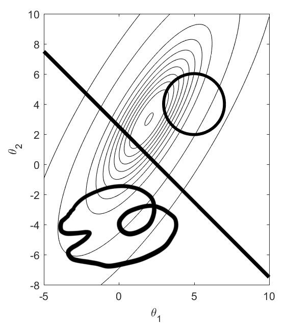
Figure 1: Level curves for a bivariate fiducial together with three possible curves for restriction on the parameter space.

For the first case Fisher derives a fiducial by first proving that the projection on the line is a sufficient statistic. This follows from the factorization theorem. The resulting fiducial is the normal distribution on the line centered at the projection point with unit variance.

For the second case Fisher derives a fiducial by conditioning on the ancillary given by the distance $a$ from the center of the circle to the observed point. The resulting fiducial is the von Mises distribution centered at the projection point with a concentration parameter $\kappa=aR$ (Mardia and Jupp, 2000).

For the third and most general case Fisher (1973, p.142) writes:

In such cases rational inference is effectively completed by the calculation of the Mathematical Likelihood for each plausible position of the unknown point.

In the first two cases, and also in the general it seems, the fiducial as identified by Fisher is simply given by a normalization of the likelihood to the given curve. In the first two cases the fiducial is also given by the conditional distribution of the unrestricted fiducial to the given curve. The statistic conditioned on must have the set of parallel lines respectively concentric circles as level sets, and this defines then a unique conditional fiducial model. Furthermore, the fiducial coincides with the Bayesian posterior from the uniform prior, and is also a confidence distribution in these two cases.

Different conditional laws on these curves can be obtained without this requirement. This was demonstrated originally by Kolmogorov (1933) in his marginalization paradox on the sphere, but the same holds in the plane. Consider in particular the case where the coordinates are chosen such that the line is given by $\theta_{1}=\theta_{2}=\mu$. The result of Fisher is then obtained by conditioning on $\theta_{1}-\theta_{2}=0$. A different result is obtained by conditioning on $\theta_{1}/\theta_{2}=1$. The latter is the choice that follows from a model where $\mu$ is a scale parameter.

It can be concluded more generally that the fiducial is uniquely given if the restricting condition is specified by the value of a particular parameter as just exemplified. A source for non-uniqueness is then given by the choice of a parameter to condition on. The parameter $\theta_{1}-\theta_{2}$ and the parameter $\theta_{1}/\theta_{2}$ can both be used to ensure that the fiducial equation has a solution, but the resulting fiducials on the line $\theta_{1}=\theta_{2}$ are different.

Fisher also considered the case of a semi-infinite line in the plane. In this case he argues differently and concludes that the fiducial is given by the normal distribution on the line as before, but with a point mass at the terminal point to ensure normalization (Fisher, 1973, p.140,eq.116). This is a confidence distribution corresponding to a simple restriction of the usual unrestricted confidence intervals.

An alternative fiducial, and this coincides with the definition given before equation (22), can be obtained by conditioning on that the fiducial equation for the line problem should have a solution on the semi-infinite line. This alternative fiducial is not a confidence distribution, but it is in this case a Bayesian posterior with corresponding optimality properties. This case of a semi-infinite line in the plane was the motivation for the simpler case treated in subsection 4.4.

5.2 Repeated sampling

The case of iid sampling from a distribution with a scalar parameter can be identified with a conditional simple fiducial model as explained next. Consider a family of strictly monotonic fiducial models

$$x_{i}=\chi(u_{i},\theta_{i})$$ (25)

where each component model is as in Theorem 1. The corresponding joint fiducial model for $x=(x_{1},\ldots,x_{n})$ has a corresponding conditional fiducial model defined by the condition $C(\theta)=(\theta_{2}/\theta_{1},\theta_{3}/\theta_{1},\ldots)=(1,\ldots,1)$. This function $C$ and the value $c=(1,\ldots,1)$ is here assumed to be a part of the specification of the conditional fiducial model. The resulting fiducial is unique from the fiducial model (25) and the condition $C=c$.

For this case it is possible to calculate the fiducial density by introducing new coordinates $\alpha_{1}=\theta_{1},\alpha_{2}=\theta_{2}/\theta_{1},\ldots$. The resulting fiducial density for the conditional fiducial model is

$$c(\alpha\operatornamewithlimits{{\mid}}x)=K\alpha^{n-1}\prod_{i}\left|\partial_{\alpha}F(x_{i}\operatornamewithlimits{{\mid}}\alpha)\right|$$ (26)

where $K$ is a normalization constant, and $\alpha^{n-1}$ is the Jacobian from the change-of-variables.

If the condition is replaced by $C(\theta)=(\theta_{2}-\theta_{1},\theta_{3}-\theta_{1},\ldots)=0$, then the above $K\alpha^{n-1}$ must be replaced by $K$. It can be noted that the resulting fiducial distributions that follow by these two arguments coincide with classical results for scale and location models. This is no coincidence, and will be discussed further in subsection 5.3.

An alternative concrete example is given by equation (15) for independent samples from the gamma distribution with known scale $\beta$ and unknown shape parameter $\theta_{i}=\alpha$. The result is then two alternative fiducial distributions for the shape parameter in addition to the one resulting from the Bartlett statistic. We do not know if there exists a third condition $C$ which would reproduce the fiducial from the Bartlett statistic.

Let $f=F^{\prime}$ be the corresponding density of the statistical model that follows from equation (25). Hannig (2009, p.506) recommends to use the following fiducial density:

$$c(\alpha\operatornamewithlimits{{\mid}}x)=K\sum_{i}f(x_{1}\operatornamewithlimits{{\mid}}\alpha)\cdots f(x_{i-1}\operatornamewithlimits{{\mid}}\alpha)\left|\partial_{\alpha}F(x_{i}\operatornamewithlimits{{\mid}}\alpha)\right|f(x_{i+1}\operatornamewithlimits{{\mid}}\alpha)\cdots f(x_{n}\operatornamewithlimits{{\mid}}\alpha)$$ (27)

It is obtained by formally applying Bayes rule with a data dependent prior

$$\pi(\alpha,x)=\sum_{i}\frac{\left|\partial_{\alpha}F(x_{i}\operatornamewithlimits{{\mid}}\alpha)\right|}{f(x_{i}\operatornamewithlimits{{\mid}}\alpha)}$$ (28)

This formula was obtained from the fiducial model (25) by additional assumptions and suitable changes of variables to simplify the conditioning. The conditioning is defined differently by Hannig (2013): Instead of conditioning on $\Theta$ he conditions on $U$ given that equation (25) should have a solution with $\alpha=\theta_{i}$ for all $i$. A related approach is discussed further in subsection 5.3 below. In all cases one has to add assumptions to equation (25) in order to get a unique fiducial.

It is noteworthy that in the case $n=1$ the formula (27) reduces to the one given by Fisher (1930), and it is uniquely given by the statistical model. It can also be noted that the resulting fiducial from equation (27) in location and scale models coincide with the results found above.

The previous gives four distinct alternative fiducial distributions for the shape parameter of the gamma distribution. The fiducial described initially and obtained from the Bartlett statistic in subsection 4.2 has the advantage of being an exact confidence distribution and the presented algorithm gives iid samples directly. Samples from the three alternatives here can be produced by Markov Chain Monte Carlo methods.

5.3 Group models and conditioning

Consider a fiducial model

$$x=\chi(u,\theta)$$ (29)

as in equation (3), but now in a situation where a solution $\hat{\theta}(u,x)$ need not exist for all $(u,x)$. One way to solve this is to introduce an enlarged fiducial model

$$x=\chi^{*}(u,\theta^{*})$$ (30)

with $\theta^{*}\in\Omega_{\Theta^{*}}\supset\Omega_{\Theta}$, $\chi^{*}(u,\theta)=\chi(u,\theta)$, a guaranteed solution $\hat{\theta}^{*}(u,x)$, and a condition $C(\theta^{*})=c$ such that

$$\Omega_{\Theta}=(C=c)=\{\theta^{*}\operatornamewithlimits{{\mid}}C(\theta^{*})=c\}$$ (31)

This gives a fiducial distribution, but it depends on the specific construction and in particular on the condition $C=c$ as exemplified in the previous two subsections.

An example of this approach is given by the fiducial model

$$x=u+\theta$$ (32)

where $x$ and $u$ belongs to a Hilbert space $\Omega_{X}$, and $\theta$ belong to a subspace $\Omega_{\Theta}\subset\Omega_{X}$. In this case a solution $\theta$ does not exist for all $(u,x)$, but a solution $\hat{\theta}^{*}(u,x)=x-u$ exists in $\Omega_{\Theta^{*}}=\Omega_{X}$. The corresponding conditional enlarged natural fiducial model gives the fiducial

$$(\Theta^{*}\operatornamewithlimits{{\mid}}C(\Theta^{*})=0)\sim(x-U\operatornamewithlimits{{\mid}}C(x-U)=0)\sim(x-U\operatornamewithlimits{{\mid}}C(U)=C(x))$$ (33)

where $C$ is the projection on the orthogonal complement of $\Omega_{\Theta}$.

In the previous example it was demonstrated that a condition on $\Theta^{*}$ was equivalent with a condition on $U$. This will always be the case if the extended model (30) defines a one-one correspondence between $u$ and $\theta^{*}$ for each $x$. The conditioning in the example is also equivalent to the conditional statistical model obtained by the condition

$$C(X)=c(x)$$ (34)

since $C(X)=C(U+\theta)=C(U)$. This is then an example of conditional inference given an ancillary statistic $C$. Conditional inference can be debatable in general, but in the present case the result is still optimal inference in a frequentist sense (Taraldsen and Lindqvist, 2013).

The previous example for a subspace of a Hilbert space generalizes verbatim to the case of a group model where the parameter space is a subgroup acting on a larger group and $C$ is a maximal invariant group homomorphism (Taraldsen and Lindqvist, 2013).

6 Discussion

Historically, up to the present date, the most important development motivated by the seminal paper by Fisher (1930) is given by the theory of confidence intervals and hypothesis testing as developed by Neyman (1937). Birnbaum (1961) introduced the concept of a confidence curve to represent confidence intervals or regions simultaneously for all confidence levels as suggested by others (Tukey, 1949; Cox, 1958). Based on these ideas Schweder (2007) introduces the concept of a confidence net $N$ which is a stochastic function from parameter space to the unit interval. The defining assumption $N(\theta)\sim\mathop{Uniform}(0,1)$ ensures that $(N\leq\alpha)=\{\theta\operatornamewithlimits{{\mid}}N(\theta)\leq\alpha\}$ is an $\alpha$-level confidence region.

An example of a confidence net is given by $\theta\mapsto N(\theta)=F(X;\theta)$ from equation (1) and the assumptions made by Fisher. A reformulation along the lines of Blaker (2000) shows that this can be seen as a direct generalization of equation (1) in that both the parameter and the data can be completely arbitrary. Both Blaker (2000) and Schweder (2007) give explicit and quite general methods that can be used for the construction of confidence nets.

The previous gives the initial ingredients for a general theory of confidence distributions for a general parameter space. A confidence net can be obtained from a confidence distribution together with a specific confidence region method. Examples can be given to show that there exist many different confidence nets arising from a given confidence distribution.

The concept of a fiducial distribution, as defined in this paper in Section 3, can be used to produce examples of confidence distributions in multiparameter cases. We prefer, however, to use the term fiducial also for cases where it is not interpretable as a confidence distribution. This is in harmony with the final words written on the subject matter by Fisher (1973, p.54-55):

By contrast, the fiducial argument uses the observations only to change the logical status of the parameter from one in which nothing is known of it, and no probability statement about it can be made, to the status of a random variable having a well-defined distribution.

One of the best textbook source on the fiducial controversy known to the authors is the classic text by Stuart et al. (1999). They discuss in particular various non-uniqueness controversies arising from the fiducial argument when generalized to the multiparameter case. One line of arguments focus on pivotal quantities, and the above discussion of confidence nets can be seen as a continuation of this line of thoughts. Uniqueness of a confidence distribution is not generally possible, but in good situations it can be unique given suitable additional optimality criteria (Schweder and Hjort, 2016). An alternative line of arguments focus on the fiducial as a substitute for a Bayesian posterior in cases without prior information. Again, general uniqueness seem out of reach, and work remains to be done on foundational issues.

Equation (3) represents a common ingredient in most recent (Hannig et al., 2016), and also many older (Fraser, 1968; Dempster, 1968; Fraser, 1979; Dawid and Stone, 1982) developments of the original fiducial argument of Fisher (1930). There are essentially two basic complications that may arise:

1. The solution with respect to the parameter is non-unique.

2. There is no solution.

Complication 1 can be seen as the source for the development of the Dempster-Shafer theory (Shafer, 2008). An alternative solution (Hannig, 2013) is given by the additional introduction of a randomization rule that chooses among the solutions allowed by equation (3).

Complication 2 can intuitively be solved by conditioning on the existence of a solution. This is, unfortunately, in many cases of interest technically challenging since the conditioning event may have zero probability and non-uniqueness may arise as in the original Borel paradox described by Kolmogorov (1933). The most appealing approach known to the authors for solving this is represented by work by Hannig (2013). He considers the model as a limit of discretized models. It has been demonstrated convincingly in many papers that this can lead to very good inference procedures in problems otherwise out of reach (Hannig et al., 2016).

The conditional fiducial models introduced here can in certain cases, as a by-product, present an alternative solution to complication 2 as shown. Existence and uniqueness follows then without the technical measure theoretic complications inherent in the more general and applicable approach presented by Hannig et al. (2016). The definition of a conditional fiducial model as given before equation (22) is, however, not intended as a general solution to complication 2. The main motivation behind the definition is as described in relation to the original examples given by Fisher (1973).

According to Pedersen (1978, p.147) the fiducial argument has had a very limited success and was then in 1978 essentially dead. Now, in 2017, there are several recent publications indicating that the fiducial argument is still very much alive and can be used successfully in both theoretical and practical directions (Efron, 1998; Schweder and Hjort, 2002; Lidong et al., 2008; Wang and Iyer, 2009; Frenkel, 2009; Taraldsen and Lindqvist, 2013; Xie and Singh, 2013; Hannig, 2013; Martin and Liu, 2014; Veronese and Melilli, 2014; Yang et al., 2014; Nadarajah et al., 2015; Taraldsen and Lindqvist, 2015; Hannig et al., 2016). The main contributions in this paper can be summarized by the following.

• Uniqueness of the fiducial distribution in a restricted class of models is proved in Theorem 1.

• The concept of a conditional fiducial model is introduced.

• Examples relating the above two points have been presented together with examples that show its historical origin by reference to the final work on this by Fisher (1973).

References

References

- Berger et al. (2009) J. O. Berger, J. M. Bernardo, and D. Sun. The Formal Definition of Reference Priors. The Annals of Statistics, 37(2), 2009.
- Bernardo (1979) J. M. Bernardo. Reference Posterior Distributions for Bayesian Inference. J. Roy. Statist. Soc. Ser. B, 41(2), 1979.
- Birnbaum (1961) A. Birnbaum. Confidence curves: An omnibus technique for estimation and testing statistical hypotheses. Journal of the American Statistical Association, 56(294):246–249, 1961.
- Blaker (2000) H. Blaker. Confidence curves and improved exact confidence intervals for discrete distributions. Can J Statistics, 28(4):783–798, 2000.
- Bølviken and Skovlund (1996) E. Bølviken and E. Skovlund. Confidence Intervals from Monte Carlo Tests. Journal of the American Statistical Association, 91(435):1071–1078, 1996.
- Cisewski and Hannig (2012) J. Cisewski and J. Hannig. Generalized fiducial inference for normal linear mixed models. Annals of Statistics, 40(4):2102–2127, 2012.
- Cox (1958) D. R. Cox. Some problems connected with statistical inference. Annals of Mathematical Statistics, 29:357–72, 1958.
- Dawid and Stone (1982) A. P. Dawid and M. Stone. The functional-model basis of fiducial inference (with discussion). The Annals of Statistics, 10(4):1054–1074, 1982.
- Dempster (1968) A. P. Dempster. A Generalization of Bayesian Inference (with discussion). J. Roy. Statist. Soc. Ser. B, 30(2):205–247, 1968.
- Efron (1998) B. Efron. R. A. Fisher in the 21st century (with discussion). Statistical Science, 13:95–122, 1998.
- Fisher (1915) R. A. Fisher. Frequency distribution of the values of the correlation coefficent in samples from an indefinitely large population. Biometrika, 10:507–21, 1915.
- Fisher (1930) R. A. Fisher. Inverse probability. Proc. Camb. Phil. Soc., 26:528–535, 1930.
- Fisher (1950) R. A. Fisher. Contributions to mathematical statistics (Wiley publications in statistics). Wiley, New York, 1st edition, 1950.
- Fisher (1973) R. A. Fisher. Statistical methods and scientific inference. Hafner press, 1973.
- Fraser (1968) D. A. S. Fraser. The structure of inference. John Wiley, 1968.
- Fraser (1979) D.A.S. Fraser. Inference and Linear Models. McGraw-Hill, 1979.
- Frenkel (2009) R. B. Frenkel. Fiducial inference applied to uncertainty estimation when identical readings are obtained under low instrument resolution. Metrologia, 46(6):661–667, 2009.
- Hannig (2009) J. Hannig. On generalized fiducial inference. Statistica Sinica, 19(2):491–544, 2009.
- Hannig (2013) J. Hannig. Generalized Fiducial Inference via Discretization. Statistica Sinica, 23:489–514, 2013.
- Hannig et al. (2007) J. Hannig, H. K. Iyer, and C. M. Wang. Fiducial approach to uncertainty assessment accounting for error due to instrument resolution. Metrologia, 44(6), 2007.
- Hannig et al. (2016) J. Hannig, H. Iyer, R.C.S. Lai, and T.C.M. Lee. Generalized fiducial inference: A review and new results. Journal of the American Statistical Association, 111(515):1346–1361, 2016.
- Jaynes (2003) E. T. Jaynes. Probability Theory: The Logic of Science. Cambridge University Press, 2003.
- Jeffreys (1946) H. Jeffreys. An invariant form for the prior probability in estimation problems. Proc.Roy.Soc. A, 186:453–461, 1946.
- Kolmogorov (1933) A. Kolmogorov. Foundations of the theory of probability. Chelsea edition (1956), second edition, 1933.
- Lidong et al. (2008) E. Lidong, J. Hannig, and H. Iyer. Fiducial Intervals for Variance Components in an Unbalanced Two-Component Normal Mixed Linear Model. Journal of the American Statistical Association, 103(482):854–865, 2008.
- Lillegård and Engen (1999) M. Lillegård and S. Engen. Exact confidence intervals generated by conditional parametric bootstrapping. Journal of Applied Statistics, 26(4):447–459, 1999.
- Lindqvist and Taraldsen (2005) B. H. Lindqvist and G. Taraldsen. Monte Carlo conditioning on a sufficient statistic. Biometrika, 92(2):451–464, 2005.
- Mardia and Jupp (2000) K. V. Mardia and P. E. Jupp. Directional Statistics. Wiley, 2000.
- Martin and Liu (2014) R. Martin and C. Liu. Foundations of statistical inference, revisited. Statistical Science, 29(2):247–251, 2014.
- Nadarajah et al. (2015) S. Nadarajah, S. Bityukov, and N. Krasnikov. Confidence distributions: A review. Statistical Methodology, 22:23–46, 2015.
- Neyman (1937) J Neyman. Outline of a theory of statistical estimation based on the classical theory of probability. Philosophical Transactions of the Royal Society of London. Series A, Mathematical and Physical Sciences, 236(767):333–380, 1937.
- Pedersen (1978) J. G. Pedersen. Fiducial Inference. International Statistical Review / Revue Internationale de Statistique, 46(2):147–170, 1978.
- Reid (2003) N. Reid. Asymptotics and the theory of inference. The Annals of Statistics, 31(6):1695–1731, 2003.
- Schweder (2007) T. Schweder. Confidence nets for curves. In V. Nair, editor, Advances in statistical modeling and inference. Essays in Honor of Kjell A Doksum, pages 593–609. World Scientific, 2007.
- Schweder and Hjort (2002) T. Schweder and N. L. H. Hjort. Confidence and Likelihood. Scandinavian Journal of Statistics, 29:309–332, 2002.
- Schweder and Hjort (2016) T. Schweder and N.L. Hjort. Confidence, Likelihood, Probability: Statistical Inference with Confidence Distributions. Cambridge University Press, 2016.
- Seidenfeld (1992) T. Seidenfeld. R. A. Fisher’s Fiducial Argument and Bayes’ Theorem. Statistical Science, 7(3):358–368, 1992.
- Shafer (2008) Glenn Shafer. Belief Functions and Parametric Models. In RolandR Yager and Liping Liu, editors, Classic Works of the Dempster-Shafer Theory of Belief Functions, volume 219 of Studies in Fuzziness and Soft Computing, pages 265–290. Springer Berlin Heidelberg, 2008.
- Stuart et al. (1999) A. Stuart, K. Ord, and S. Arnold. Kendall’s Advanced Theory of Statistics, Classical Inference and the Linear Model, volume 2A. Wiley, sixth edition, 1999.
- Taraldsen (2006) G. Taraldsen. Instrument resolution and measurement accuracy. Metrologia, 43:539–544, 2006.
- Taraldsen and Lindqvist (2013) G. Taraldsen and B. H. Lindqvist. Fiducial theory and optimal inference. Annals of Statistics, 41(1):323–341, 2013.
- Taraldsen and Lindqvist (2015) G. Taraldsen and B. H. Lindqvist. Fiducial and Posterior Sampling. Communications in Statistics: Theory and Methods, 44(17):3754–3767, 2015.
- Taraldsen and Lindqvist (2016) G. Taraldsen and B. H. Lindqvist. Conditional probability and improper priors. Communications in Statistics: Theory and Methods, 45(17):5007–5016, 2016.
- Tukey (1949) J. W. Tukey. Standard confidence points. Memorandum Report 26, Statistical Research Group, 1949.
- Veronese and Melilli (2014) P. Veronese and E. Melilli. Fiducial and Confidence Distributions for Real Exponential Families. Scandinavian Journal of Statistics, 2014.
- Wang and Iyer (2009) C. M. Wang and H. K. Iyer. Fiducial intervals for the magnitude of a complex-valued quantity. Metrologia, 46(1):81–86, 2009.
- Wilkinson (1977) G. N. Wilkinson. On resolving the controversy in statistical inference. Journal of the Royal Statistical Society. Series B (Methodological), 39(2):119–171, 1977.
- Xie and Singh (2013) M. Xie and K. Singh. Confidence Distribution, the Frequentist Distribution Estimator of a Parameter: A Review. International Statistical Review, 81(1):3–39, 2013.
- Yang et al. (2014) G. Yang, D. Liu, R. Y. Liu, M. Xie, and D. C. Hoaglin. Efficient network meta-analysis: A confidence distribution approach. Statistical Methodology, 20:105–125, 2014.