Non-standard interactions and neutrinos from dark matter annihilation in the Sun

Abstract

We perform an analysis of the influence of non-standard neutrino interactions (NSI) on neutrino signal from dark matter annihilations in the Sun. Taking experimentally allowed benchmark values for the matter NSI parameters we show that the evolution of such neutrinos with energies at GeV scale can be considerably modified. We simulate propagation of neutrinos from the Sun to the Earth for realistic dark matter annihilation channels and find that the matter NSI can result in at most 30% correction to the signal rate of muon track events at neutrino telescopes. Still present experimental bounds on dark matter from these searches are robust in the presence of NSI within considerable part of their allowed parameter space. At the same time electron neutrino flux from dark matter annihilation in the Sun can be changed by a factor of few.

1 Introduction

Dark matter is one of the most intriguing mysteries of the modern particle physics. Existence of new particles is the dominant hypothesis for explanation of this phenomena [1]. Looking for neutrinos resulting from dark matter annihilation in the Sun is one of the possible indirect way of searching for the signal from dark matter particles [2]. The idea is that these particles can be gravitationally trapped and accumulated inside the Sun [3] during its evolution in such amount that they start to annihilate. If dark matter particles annihilate into SM particles than among the final products of these annihilations can be high energy neutrinos which can reach the surface of the Sun, traverse to the Earth and be observed at neutrino telescopes such as IceCube [4], Super-Kamiokande [5], ANTARES [6] as well as neutrino telescopes at the Baksan [7] and Baikal [8].

A lot of physical processes are involved in this scenario. The capture process crucially depends on the mass of dark matter particles $m_{DM}$ and the size of cross section of nonrelativistic elastic scattering of dark matter with nucleons. In particular, effective capture is possible only for dark matter particles heavier than about 3–5 GeV. Otherwise, evaporation of dark matter from the Sun is important [9]. Dark matter particles can annihilate over different annihilation channels, which is very model-dependent. Instead of considering a particular model it is common to work with a chosen set of annihilation channels which are believed to capture the main features of the general picture. Standard benchmark annihilation channels are $b\bar{b}$ channel with very soft spectrum of neutrinos, $W^{+}W^{-}$ and $\tau^{+}\tau^{-}$ channels with more energetic spectra as well as monochromatic neutrino channels $\nu\bar{\nu}$. Each annihilation channels provides not only with unique neutrino energy spectrum but also with a particular flavor content. Thus, different neutrino signals can be expected from different annihilation channels.

Produced neutrinos propagate in the Sun, from the Sun to the Earth and in the Earth to neutrino telescope. In most experimental searches of this type muon neutrinos are the most important and their expected flux at the detector level is given by the following expression

$$\Phi_{\nu_{\mu}}=\frac{\Gamma_{A}}{4\pi R^{2}}\times\sum_{\nu_{\alpha},\bar{\nu_{\alpha}}}\int_{E_{th}}^{m_{DM}}dE_{\nu_{\alpha}}P_{\alpha\mu}(E_{\nu_{\alpha}},E_{th})\frac{dN^{\rm prod}_{\nu_{\alpha}}}{dE_{\nu_{\alpha}}}\;,$$ (1.1)

where $\Gamma_{A}$ is dark matter annihilation rate, $R$ is the distance from the Sun to the Earth, $E_{th}$ is neutrino threshold energy, $\frac{dN^{\rm prod}_{\nu_{\alpha}}}{dE_{\nu_{\alpha}}}$ is neutrino energy spectrum at production and the function $P_{\alpha\mu}(E_{\nu_{\alpha}},E_{th})$ is the probability of obtaining muon (anti)neutrino in the detector from (anti)neutrino of given flavor $\alpha$ at production which encodes all effects of neutrino propagation. This last can be quite nontrivial and it depends on neutrino oscillations, charge current (CC) and neutral current (NC) interactions of neutrino interactions with matter.

On Figure 1 we show the probability for (anti)neutrino

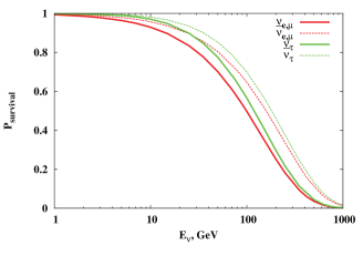
Figure 1: Survival probability of neutrino and antineutrino of different flavors produced in the center of the Sun.

of a particular flavor to escape the Sun at the same energy, calculated without oscillations, i.e. survival probability; see Ref. [10] for similar picture. One can see that the absorption effect is small for neutrino of energies less than 10 GeV and very crucial for neutrino with energy larger than about 100 GeV. Oscillations also produce dramatic effect. Comparing integrated final muon neutrino fluxes at the Earth level calculated with and without oscillation effects (see e.g. right panel of Fig. 10 in Ref. [7]) one observes that the effect of neutrino oscillations varies from 10–40% for $b\bar{b}$ and $W^{+}W^{-}$ annihilation channel to factor of 3.5 for dark matter annihilations into $\tau^{+}\tau^{-}$. This indicates that new physics which influences neutrino interactions and oscillations could also affect propagation of neutrinos from dark matter annihilations in the Sun and change corresponding neutrino signal. Studies in this direction was performed recently in Refs. [11, 12] where effect of light sterile neutrino on the signal from dark matter annihilation in the Sun was discussed.

In this paper we study influence of the non-standard interactions (NSI) of neutrino with matter [13] on neutrino signal from dark matter annihilations in the Sun. Such interactions appear in different types of models of new physics, see e.g. [14]. Neutrino NSI attract recently much attention and several studies were performed scrutinizing their different aspects, see Refs. [15, 16, 17] for reviews. NSI can potentially influence propagation of solar neutrinos [18, 19, 20, 21], neutrinos from supernova [22, 23], atmospheric neutrinos [24, 25, 26, 27, 28, 29, 30, 31, 32, 33, 34], neutrinos from artificial sources [35, 36, 37, 38, 39, 40, 41, 42, 43, 44, 45, 46, 47] as well as reveal themselves in different production and decay processes [48, 49, 50]. In particular, matter NSI can produce “missing energy” signature at collider experiments and in particular at the LHC [51, 52] although interpretation of these results may be quite model dependent.

Here we study effect of the matter NSI on propagation of high energy neutrinos from dark matter annihilation in the Sun. We find that for realistic annihilation channels and phenomenologically allowed values of NSI parameters, deviations of neutrino flux at the Earth level from the standard (no-NSI) case can be considerable. The rest of the paper is organized as follows. In Section 2 we briefly remind the main facts about the matter NSI which are relevant for the present analysis, i.e. parameters, influence on neutrino oscillations and current experimental bounds. In Section 3 we consider evolution of monochromatic neutrinos from dark matter annihilations in the Sun. To single out effect of the matter NSI, in this Section we neglect all neutrino interactions except for the forward neutrino scattering. Turning on the matter NSI we numerically simulate evolution of neutrinos from the Sun to the Earth and supply this analysis with simplified analytical study. In Section 4 we perform full Monte-Carlo simulations of neutrino propagation which includes neutrino interactions. We consider $b\bar{b},W^{+}W^{-}$ and $\tau^{+}\tau^{-}$ annihilation channels and estimate the effect of different NSI parameters on the muon track event rate at neutrino telescopes. Section 5 contains our conclusions.

2 NSI and modification of neutrino propagation

At sufficiently low transverse momenta the matter NSI of neutrino can be described by the following effective lagrangian

$${\cal L}^{NC}_{NSI}=-\sum_{f,P=P_{L},P_{R}}\epsilon_{\alpha\beta}^{fP}2\sqrt{2}G_{F}(\bar{\nu}_{\alpha}\gamma^{\mu}P_{L}\nu_{\beta})(\bar{f}\gamma_{\mu}Pf).$$ (2.1)

Here $P_{L,R}$ are chirality projectors, $\epsilon_{\alpha\beta}^{fP}$ are the NSI parameters and sum is implied over all SM fermions $f$. Let us note that apart from the neutral current type of NSI in (2.1) in general one can introduce NSI of charge current type. Their main impact would be to affect neutrino CC interaction cross sections. Present experimental bounds on the parameters of the charged current type of NSIs are quite severe [15]; we expect that their effect on high-energy neutrino propagation in the Sun and the Earth would be small and focus on the influence of the matter NSIs. One of the main consequences of the interactions (2.1) is modification of neutrino propagation through matter. Evolution of relativistic neutrino in media can be described by the following Hamiltonian

$$H=\frac{1}{2E_{\nu}}U{\rm diag}(m_{1}^{2},m_{2}^{2},m_{3}^{2})U^{\dagger}+V_{e}\epsilon^{m},$$ (2.2)

where $m_{i}^{2},i=1,2,3$ are neutrino masses squared, $U$ is the vacuum Pontecorvo-Maki-Nakagawa-Sakata (PMNS) matrix and $E_{\nu}$ is neutrino energy. We use standard parametrization of the PMNS matrix (omitting Majorana phases)

$$U=R_{23}(\theta_{23})U_{\delta}^{\dagger}R_{13}(\theta_{13})U_{\delta}R_{12},$$ (2.3)

where $R_{ij}$ is rotation matrix in $ij$-plane and $U_{\delta}$ is phase matrix containing CP-violating parameter

$$U_{\delta}=\left(\begin{array}[]{ccc}e^{i\delta/2}&0&0\\ 0&1&0\\ 0&0&e^{-i\delta/2}\end{array}\right).$$ (2.4)

Further for numerical calculations we use the values of oscillation parameters presented in Table 1

	$\Delta m_{21}^{2}$, eV2	$|\Delta m_{31}^{2}|$, eV2	$\sin^{2}{\theta_{12}}$	$\sin^{2}{\theta_{23}}$	$\sin^{2}{\theta_{13}}$	$\delta_{CP}$
NH	$7.50\cdot 10^{-5}$	$2.457\cdot 10^{-3}$	0.304	0.452	0.0218	0
IH	$7.50\cdot 10^{-5}$	$2.449\cdot 10^{-3}$	0.304	0.579	0.0219	0

Table 1: Neutrino oscillation parameters used for the present analysis [53].

for normal (NH) and inverted (IH) hierarchy. These parameters lie within $3\sigma$ range of their experimentally allowed values [53]. For simplicity we assume CP-violating phase to be zero. The matter term in (2.2) contains a factor $V_{e}\equiv\sqrt{2}G_{F}N_{e}$ for neutrino and $V_{e}\equiv-\sqrt{2}G_{F}N_{e}$ for antineutrino. This term is proportional to the electron number density $N_{e}$ and the matrix

$${\epsilon}^{m}=\left(\begin{array}[]{ccc}1+{\epsilon}_{ee}&{\epsilon}_{e\mu}&{\epsilon}_{e\tau}\\ {\epsilon}_{e\mu}^{*}&{\epsilon}_{\mu\mu}&{\epsilon}_{\mu\tau}\\ {\epsilon}_{e\tau}^{*}&{\epsilon}_{\mu\tau}^{*}&{\epsilon}_{\tau\tau}\end{array}\right),$$ (2.5)

describing influence of the matter NSI as well as the Standard Model contribution. The NSI parameters ${\epsilon}_{\alpha\beta}$ depend on coupling constants in the lagrangian (2.1) and on the matter content as follows

$${\epsilon}_{\alpha\beta}=\sum_{f=e,u,d}({\epsilon}_{\alpha\beta}^{fP_{L}}+{\epsilon}_{\alpha\beta}^{fP_{R}})\frac{N_{f}}{N_{e}},$$ (2.6)

where $N_{f}$ is the number density of the fermion $f$. Model independent experimental bounds on parameters ${\epsilon}_{\alpha\beta}$ are presented below

$$|{\epsilon}_{\alpha\beta}^{\rm Earth}|<\left(\begin{array}[]{ccc}4.2&0.33&3.0\\ ...&0.068&0.33\\ ...&...&21.0\end{array}\right),\;\;\;|{\epsilon}_{\alpha\beta}^{\rm Sun}|<\left(\begin{array}[]{ccc}2.5&0.21&1.7\\ ...&0.046&0.21\\ ...&...&9.0\end{array}\right)$$ (2.7)

for the Earth-like and Sun-like matter, see Refs. [15, 54]. There are more restrictive bounds on some of the Earth NSI parameters coming from results of the Super-Kamiokande [55] experiment

$$|{\epsilon}^{\rm Earth}_{\mu\tau}|<0.033,\;\;\;|{\epsilon}^{\rm Earth}_{\tau\tau}-{\epsilon}^{\rm Earth}_{\mu\mu}|<0.147.$$ (2.8)

Even stronger bounds on the values of $|{\epsilon}^{\rm Earth}_{\mu\tau}|$ (up to 0.02) were obtained [27, 34, 56] from the results of IceCube. Experimental bounds on the NSI parameters ${\epsilon}_{\alpha\beta}^{fP}$ from neutrino scattering experiments was discussed in Refs. [15, 16, 17] in details. Effects of the matter NSI for existing and upcoming neutrino experiments was discussed in many papers, we refer here to a review paper [17].

Let us note that not only matter NSI parameters for the Earth can be different from those for the Sun, but also ${\epsilon}_{\alpha\beta}^{Sun}$ are position dependent because the matter content in the Sun changes from the center to the surface. Namely, the proton-to-neutron ratio $\frac{N_{p}}{N_{n}}$ varies from about 2 at the center to about 6 near the surface. Analysis of the most general case lies beyond the scope of the present study in which we are going to illustrate the main effects of the matter NSI on propagation of neutrinos in the Sun and the Earth. In what follows for simplicity we limit ourselves by the case of position independent values of ${\epsilon}^{Sun}_{\alpha\beta}$ and consider the simplifying situation with ${\epsilon}_{\alpha\beta}^{Earth}={\epsilon}_{\alpha\beta}^{Sun}\equiv{\epsilon}_{\alpha\beta}$.

In general the NSI (2.1) could modify the NC neutrino-nucleon interaction cross section which could affect neutrino propagation in the Sun and the Earth. In what follows we neglect this effect because its influence on the final neutrino flux will be subleading to the standard NC and CC neutrino interactions for chosen values of the matter NSI parameters. We leave the detailed analysis of this effect for future study.

3 Evolution of monochromatic WIMP neutrinos in the Sun and Earth

Propagation of high energy neutrinos from dark matter annihilations in the Sun has been studies both analytically [57, 58, 59] and numerically [10, 60, 61, 62]. In this Section we discuss effect of the matter NSI on propagation of monochromatic neutrino in the Sun and the Earth. We analyze effect of the NSI neglecting all neutrino interactions except for the forward neutrino scattering which directly affects neutrino oscillations. Bearing in mind muon track signature at neutrino telescopes in what follows we consider neutrino energy range from 1 GeV to 1 TeV. The lowest bound is determined mainly by muon energy thresholds for such searches in neutrino experiments (about 1.5 GeV for Super-Kamiokande and about 1 GeV for Baksan Underground Neutrino Telescope). At the same time, neutrinos with energies larger than 1 TeV have very small probability to escape the Sun, see Fig. 1. We numerically solve Schrodinger equation with the Hamiltonian (2.2) for realistic electron density profiles in the Sun [67] and the Earth [68]. Varying density of the Sun has been taken into account in the following way: we divide neutrino path in sufficiently small pieces in which electron density can be considered as a constant and then evolve neutrino wave function with exact evolution operator. We use the algorithm described in Refs. [69, 70] to simulate neutrino oscillations in $3\times 3$ scheme. We assume that neutrinos are produced near the center of the Sun in a flavor state $\nu_{\alpha}$. Production region of the neutrinos in the Sun follows expected dark matter distribution [71] (see also [72] for recent study)

$$n(r)=n_{0}\,e^{-r^{2}/R_{DM}^{2}},\;\;{\rm with}\;\;R_{DM}\sim 0.1R_{Sun}\sqrt{\frac{1~{}{\rm GeV}}{m_{DM}}},$$ (3.1)

which depends on the mass of dark matter particle. Here $R_{Sun}$ is the radius of the Sun. Numerically, size of the DM core in the Sun varies from about $4\cdot 10^{4}$ km for $m_{DM}\sim 3$ GeV to $2.2\cdot 10^{3}$ km for $m_{DM}\sim 1$ TeV. For the case of monochromatic neutrino annihilation channels we simulate the production point according to the distribution (3.1) with $m_{DM}=E_{\nu}$. Produced neutrino evolves according to the Schrodinger equation with the Hamiltonian (2.2). In the analysis we take into account small ellipticity of the Earth orbit. Namely, we randomly choose time of each neutrino event (i.e. fraction of the year) and average final probabilities over positions of dark matter annihilation and the Earth.

Let us start our analysis with the standard case without NSI. On Fig. 2

Figure 2: Probabilities $P_{\mu\alpha}$ to obtain neutrino of different flavors $\nu_{\alpha}$ at the Earth orbit from $\nu_{\mu}$($\bar{\nu}_{\mu}$) in the Sun for normal (left panels) and inverted (right panels) hierarchy for ${\epsilon}_{\alpha\beta}=0$. Plots in the upper (lower) panels correspond to neutrino (antineutrino) case.

Figure 3: Probabilities to obtain neutrino of different flavors after propagation in the Earth from $\nu_{\mu}$($\bar{\nu}_{\mu}$) produced in the Sun for normal (left panels) and inverted (right panels) hierarchy for ${\epsilon}_{\alpha\beta}=0$. Plots in the upper (lower) panels correspond to neutrino (antineutrino) case.

we plot probabilities to obtain neutrinos of different flavours at the Earth orbit (i.e. no propagation in the Earth). As an illustrative example we consider here and in the subsequent Figures in this Section the case of muon (anti)neutrino at production. Left and right panels correspond to the cases of normal and inverted neutrino mass hierarchy, respectively, with the oscillation parameters taken from Table 1. The case of neutrino is shown in the upper panels, while the lower panels are reserved for antineutrinos. To average over varying neutrino baseline we simulate $N_{av}=100$ neutrino events for each value of neutrino energy. In Fig. 3 we present the same probabilities after propagation in the Earth. For illustration purposes in the Section we consider propagation though the center of the Earth only. In the next Section we relax this assumption when making full-fledged Monte-Carlo simulation of neutrino propagation.

To explain the behavior of the probabilities as functions of neutrino energy let us introduce apart from neutrino flavor states $|\nu_{\alpha}\rangle,\alpha=e,\mu,\tau$ and vacuum eigenstates $|i\rangle,i=1,2,3$ also the eigenstates of the instantaneous matter Hamiltonian as

$$|\alpha\rangle=U^{m}_{\alpha j}(r)|j_{m},r\rangle,$$ (3.2)

where $U^{m}(r)$ is the mixing matrix diagonalizing neutrino Hamiltonian in matter: $H_{m}(r)=U^{m\dagger}(r)H(r)U^{m}(r)$. In the absence of the matter NSI for high energy neutrinos corresponding eigenstates of the matter Hamiltonian (2.2) in the center of the Sun are approximately $|1_{m},0\rangle=|\nu_{e}\rangle$ and

$$|2_{m},0\rangle=c_{23}|\nu_{\mu}\rangle-s_{23}|\nu_{\tau}\rangle,\;\;\;|3_{m},0\rangle=s_{23}|\nu_{\mu}\rangle+c_{23}|\nu_{\tau}\rangle,$$ (3.3)

where we use the standard notations $c_{ij}=\cos{\theta_{ij}}$ and $s_{ij}=\sin{\theta_{ij}}$. The state $|\nu_{e}\rangle$ is decoupled in the center due to large matter contribution and produced $\nu_{\mu}$ oscillates to $\nu_{\tau}$ with the mixing angle $\theta_{23}$. If electron density changes much slower than neutrino oscillates, i.e. in the adiabatic regime, the instantaneous eigenstates are approximately evolution eigenstates and in this limit no transitions between these eigenstates occur. If the oscillation length $L_{23}=\frac{4\pi E_{\nu}}{|\Delta m_{23}^{2}|}$ is small as compared to $2R_{DM}$ then $\mu-\tau$ oscillation phase averages to zero and one obtains outside the production region a mixed state $c^{2}_{23}|2_{m},r\rangle\langle 2_{m},r|+s^{2}_{23}|3_{m},r\rangle\langle 3_{m},r|$. In the adiabatic regime the matter Hamiltonian eigenstates $|2_{m}\rangle$ and $|3_{m}\rangle$ evolve at the solar surface into some vacuum eigenstates $|i_{2}\rangle$ and $|i_{3}\rangle$, respectively. For normal mass hierarchy one obtains

$$|2_{m}\rangle\to|1\rangle,\;\;\; |3_{m}\rangle\to|2\rangle\;\;{\rm for}\;\nu\,,$$ (3.4)

$$|2_{m}\rangle\to|2\rangle,\;\;\; |3_{m}\rangle\to|3\rangle\;\;{\rm for}\;\bar{\nu}\,.$$ (3.5)

For the case of inverted hierarchy

$$|2_{m}\rangle\to|1\rangle,\;\;\; |3_{m}\rangle\to|3\rangle\;\;{\rm for}\;\nu\,,$$ (3.6)

$$|2_{m}\rangle\to|2\rangle,\;\;\; |3_{m}\rangle\to|1\rangle\;\;{\rm for}\;\bar{\nu}\,.$$ (3.7)

Finally one gets a mixed state describing by the following density matrix $c^{2}_{23}|i_{2}\rangle\langle i_{2}|+s^{2}_{23}|i_{3}\rangle\langle i_{3}|$. Probability to detect neutrino $\nu_{\beta}$ at the Earth orbit looks as follows

$$P(\nu_{\mu}\to\nu_{\beta})=c^{2}_{23}|U_{\beta\,i_{2}}|^{2}+s^{2}_{23}|U_{\beta\,i_{3}}|^{2}.$$ (3.8)

In a more generic case for neutrino $\nu_{\alpha}$ at the solar center, the neutrino state at the Earth orbit can be approximately described [57] by the density matrix

$$\rho=\sum_{i,j}\left|U_{\alpha i}^{m}(r=0)\right|^{2}P_{ij}|j\rangle\langle j|\;.$$ (3.9)

Here $P_{ij}$ are probabilities of transition between different eigenstates during evolution in the Sun. For the adiabatic evolution, $P_{ij}=\delta_{ij}$, taking convention for ordering of eigenvalues such that they smoothly approach vacuum eigenstates. Formula (3.9) assumes that statistical averaging of oscillation phases to zero takes place, which results from uncertainties in neutrino production place, small ellipticity of the Earth orbit as well as from finite energy resolution of the detector (see Ref. [57] for details). The probability to find neutrino in a flavor state $\nu_{\beta}$ at the Earth orbit from neutrino state $\nu_{\alpha}$ at production can be approximately described [57] by the following expression

$$P(\nu_{\alpha}\to\nu_{\beta})=\sum_{i,j}\left|U_{\alpha i}^{m}(r=0)\right|^{2}P_{ij}\left|U_{\beta j}\right|^{2}\;.$$ (3.10)

Adiabatic approximation may break down near Mikheyev-Smirnov-Wolfenstein (MSW) resonances [13, 73, 74]. For NH there are two MSW resonances corresponding to 1–3 and 1–2 transitions in neutrino sector and none for antineutrino. For IH one resonance 1–2 transition happens in neutrino mode while another 1–3 transition occurs for antineutrinos. Corresponding resonance conditions look  [75, 57, 76] as

$$E_{\nu}= \frac{\Delta m_{21}^{2}}{2V_{e}(r)c^{2}_{13}}\cos{2\theta_{12}}\;\;\;$$ for 1–2 resonance, (3.11)

$$E_{\nu}= \frac{\Delta m_{32}^{2}+\Delta m_{21}^{2}c^{2}{12}}{2V_{e}(r)}\cos{2\theta_{13}}\;\;\; \text{for 1--3 resonance}.$$ (3.12)

The resonance energies in the solar core lie below GeV energy scale. Adiabaticity for neutrino transitions through these resonances is violated for energies $E\mathchoice{\mathrel{\vbox{\hbox{$\buildrel\displaystyle>\over{\displaystyle\sim}$}}}}{\mathrel{\vbox{\hbox{$\buildrel\textstyle>\over{\textstyle\sim}$}}}}{\mathrel{\vbox{\hbox{$\buildrel\scriptstyle>\over{\scriptstyle\sim}$}}}}{\mathrel{\vbox{\hbox{$\buildrel\scriptscriptstyle>\over{\scriptscriptstyle\sim}$}}}}E_{NA}$, where the onset energy for nonadiabatic effects $E_{NA}$ can be estimated  [57, 75] as follows

$$E_{NA}= \frac{1}{3}\pi\bigg{|}\frac{V_{e}}{V^{\prime}_{e}}\bigg{|}_{r_{R}}\Delta m_{21}^{2}s^{2}_{12}\;\;\;$$ for 1–2 resonance, (3.13)

$$E_{NA}= \frac{1}{3}\pi\bigg{|}\frac{V_{e}}{V^{\prime}_{e}}\bigg{|}_{r_{R}}(\Delta m_{32}^{2}+\Delta m_{21}^{2}c^{2}{12})s^{2}_{13}\;\;\;$$ for 1–3 resonance, (3.14)

where $r_{R}$ is space position of the resonance. Numerically one can find that $E_{NA}$ is about 9 GeV for 1–2 resonance and about $20$ GeV for 1–3 resonance. One can check that Eq. (3.8) reproduces energy dependence of the probabilities in Fig. 2 in the low energy region. At energies larger than 10–20 GeV the evolution becomes more complicated. It happens not only due to nonadiabatic transitions through the MSW resonance regions but also because averaging of oscillation phases over production region may no longer take place. Moreover, at energies larger than 100–200 GeV oscillation lengths become comparable and even larger than ellipticity of the Earth orbit. This can result in annual modulation of the neutrino signal discussed in [59, 77]. The most important influence of subsequent propagation in the Earth (see Fig. 3) is visible for neutrino mode (NH) and antineutrino mode (IH) in the low energy region. This behavior is related mainly to 2–3 and 1–3 mixings, see [78, 79].

3.1 Flavor conserving NSI

In what follows we turn on the matter NSI parameters ${\epsilon}_{\alpha\beta}$ taking single non-zero parameter at a time. In this Section we study effect of the flavor diagonal NSI parameters. Due to smallness of the resonance energy for 1–2 transition effect of non-zero ${\epsilon}_{ee}$ within experimentally allowed region on the propagation of high energy neutrino is negligible. As a consequence effect due to small non-zero ${\epsilon}_{\mu\mu}$ will be the same as that of due to $-{\epsilon}_{\tau\tau}$. In what follows we consider non-zero value of $\epsilon_{\tau\tau}$ and assume that $\epsilon_{\tau\tau}\ll 1$ in analytical expressions which is consistent with phenomenological bounds (2.7) and (2.8). As a benchmark point we take ${\epsilon}_{\tau\tau}=\pm 0.03$. In Figs. 4 and 5 we plot probabilities to obtain neutrino of different flavors at the Earth orbit and after passing the Earth, respectively, from $\nu_{\mu}$ produced at the center of the Sun. These probabilities are calculated with ${\epsilon}_{\tau\tau}=0.03$. One can see that oscillations of neutrino in the matter of the Sun and the Earth deviates considerably from no-NSI case. Let us discuss the reasons for these deviations. In the center of the Sun the eigenstate $|1_{m},0\rangle=|\nu_{e}\rangle$ is decoupled from the others for GeV-scale neutrinos and the Hamiltonian for the rest 2–3 subsystem has the following form

$$H_{23}=\frac{\Delta m^{2}_{32}}{2E_{\nu}}R_{23}(\theta_{23})\left(\begin{array}[]{cc}0&0\\ 0&1\end{array}\right)R^{\dagger}_{23}(\theta_{23})+{\epsilon}_{\tau\tau}V_{e}\left(\begin{array}[]{cc}0&0\\ 0&1\end{array}\right).$$ (3.15)

It can be diagonalized by corresponding rotation $\nu=R_{23}(\tilde{\theta}_{23})\tilde{\nu}$, where $\tilde{\theta}_{23}$ is determined by

$$\tan{2\tilde{\theta}_{23}}=\frac{\sin{2\theta_{23}}}{\cos{2\theta_{23}}+A},$$ (3.16)

where $A=\frac{2{\epsilon}_{\tau\tau}V_{e}E_{\nu}}{\Delta m^{2}_{32}}$. When denominator in (3.16) goes to zero new 2–3 resonance occurs. The resonance energy in the center of the Sun is

$$E_{R}^{23}=-\frac{\Delta m_{32}^{2}}{2{\epsilon}_{\tau\tau}V_{e}(0)}\cos{2\theta_{23}}.$$ (3.17)

For normal mass hierarchy 2–3 resonance takes place for neutrino if ${\rm sign}({\epsilon}_{\tau\tau}\cos{2\theta_{23}})=-1$ and for antineutrino if ${\rm sign}({\epsilon}_{\tau\tau}\cos{2\theta_{23}})=+1$. For inverted mass hierarchy the resonance conditions are opposite.

Figure 4: The same as in Fig. 2 but for ${\epsilon}_{\tau\tau}=0.03$.

Figure 5: The same as in Fig. 3 but for ${\epsilon}_{\tau\tau}=0.03$.

Taking numerical values from Table 1 one obtains $E_{R}^{23}\approx 0.015/{\epsilon}_{\tau\tau}$ GeV (NH) and $E_{R}^{23}\approx 0.025/{\epsilon}_{\tau\tau}$ GeV (IH) and the resonance appears for antineutrinos in both cases. We note in passing that subsequent propagation of electron (anti)neutrino $\nu_{e}$ produced in the center of Sun is not affected by non-zero ${\epsilon}_{\tau\tau}$ (${\epsilon}_{\mu\mu}$) in the considered energy range. For relatively small values of ${\epsilon}_{\tau\tau}$ the position of 2–3 resonance is well separated in space from the other possible resonances. In this case they can be treated separately. The resonance conversion can take place only for neutrinos with $E>E_{R}^{23}$. For such neutrinos flavor states are approximately Hamiltonian eigenstates and in particular $|\nu_{\mu}\rangle$ is almost coincide with the second energy level of the matter Hamiltonian for ${\epsilon}_{\tau\tau}>0$. Adiabatic evolution through 2–3 resonance region implies

$$|\tilde{2}_{m}\rangle\to|2_{m}\rangle,\;\;\; |\tilde{3}_{m}\rangle\to|3_{m}\rangle\;\;{\rm for}\;\nu\,,$$ (3.18)

$$|\tilde{2}_{m}\rangle\to|3_{m}\rangle,\;\;\; |\tilde{3}_{m}\rangle\to|2_{m}\rangle\;\;{\rm for}\;\bar{\nu}$$ (3.19)

in the case of NH and

$$|\tilde{2}_{m}\rangle\to|3_{m}\rangle,\;\;\; |\tilde{3}_{m}\rangle\to|2_{m}\rangle\;\;{\rm for}\;\nu\,,$$ (3.20)

$$|\tilde{2}_{m}\rangle\to|2_{m}\rangle,\;\;\; |\tilde{3}_{m}\rangle\to|3_{m}\rangle\;\;{\rm for}\;\bar{\nu}\,$$ (3.21)

for IH. Let us note that onset energy for non-adiabatic effects for 2–3 transition can be estimated as follows follows [57, 75]

$$E_{NA}=\frac{1}{3}\pi\bigg{|}\frac{V_{e}}{V^{\prime}_{e}}\bigg{|}\Delta m_{32}^{2}\sin^{2}{\theta_{23}}\sim 0.5~{}{\rm TeV},$$ (3.22)

which indicates that adiabaticity for this transition is valid almost entirely in the chosen neutrino energy range. Effect of non-zero ${\epsilon}_{\tau\tau}=0.03$ is most dramatic in Fig. 4 for antineutrino (NH) and neutrino (IH). In the former case the muon antineutrino $\nu_{\mu}$ produced in the center of the Sun undergoes resonance 2–3 transition and evolves into $|3_{m}\rangle$. This state meets no level crossing in subsequent evolution to the solar surface where it becomes pure vacuum eigenstate $|3\rangle$, see (3.5). This is completely different from the evolution with no-NSI where the final state is incoherent mixture of $|2\rangle$ and $|3\rangle$, see Fig. 2. In the low energy region one should take into account an admixture of $|\tilde{3}_{m}\rangle$ state. Namely neglecting contribution of $|\tilde{1}_{m}\rangle\equiv|\nu_{e}\rangle$ one finds that

$$|\nu_{\mu}\rangle=\cos{\tilde{\theta}^{0}_{23}}|\tilde{2}_{m},0\rangle-\sin{\tilde{\theta}^{0}_{23}}|\tilde{3}_{m},0\rangle,$$ (3.23)

where $\tilde{\theta}_{23}^{0}$ is determined by Eq. (3.16) for the center of the Sun. This admixture results in deviation from simple $P_{\mu\alpha}=|U_{\alpha 3}|^{2}$ law. Similar explanation can be given for the case of neutrino (IH). For neutrino (NH) and antineutrino (IH), see Fig (4) (upper left and lower right panels), $\nu_{\mu}$ state evolve into $|2_{m},r\rangle$. For neutrino (NH) in the adiabatic regime $\nu_{\mu}$ evolves into $|1\rangle$ at the solar surface, while the evolution at higher energies is more complicated due to non-adiabatic effects. In the limit of maximal adiabaticity violation the level crossing probability approaches $c_{12}^{2}$, which corresponds to incoherent vacuum oscillations and one obtains

$$\nu_{\mu}\approx|\tilde{2}_{m}\rangle\to|2_{m}\rangle\to c^{2}_{12}|2\rangle\langle 2|+s^{2}_{12}|1\rangle\langle 1|.$$ (3.24)

For antineutrino (IH) $\nu_{\mu}$ evolves again into $|2_{m}\rangle$ state when passing 2–3 resonance and emerges as $|2\rangle$ at the Earth orbit in the adiabatic regime. At energies $E_{\nu}\mathchoice{\mathrel{\vbox{\hbox{$\buildrel\displaystyle<\over{\displaystyle\sim}$}}}}{\mathrel{\vbox{\hbox{$\buildrel\textstyle<\over{\textstyle\sim}$}}}}{\mathrel{\vbox{\hbox{$\buildrel\scriptstyle<\over{\scriptstyle\sim}$}}}}{\mathrel{\vbox{\hbox{$\buildrel\scriptscriptstyle<\over{\scriptscriptstyle\sim}$}}}}10$ GeV the main difference with no-NSI case comes from the fact that $\nu_{\mu}$ at production is only an approximate eigenstate of the matter Hamiltonian.

Let us turn to subsequent evolution in the Earth, see Fig. 5. The most prominent effect of non-zero ${\epsilon}_{\tau\tau}$ appears again for neutrino mode with inverted hierarchy and for antineutrino with normal hierarchy and reaches its culmination for $E_{\nu}\sim 30$ GeV. In this case almost pure $|3\rangle$ vacuum state reaches the Earth surface, see lower left and upper right panels on Fig. 4. Let us neglect here for simplicity small contribution of electron neutrino $\nu_{e}$ related to non-zero $\theta_{13}$. In the matter of the Earth this state is no longer Hamiltonian eigenstate and thus nontrivial evolution takes place. Eigenstates of 2–3 subsystem describing by the Hamiltonian (3.15) can be found again by rotation $\nu=R_{23}(\tilde{\theta}_{23})\tilde{\nu}$ with $\tilde{\theta}_{23}$ given by Eq. (3.16) with neutrino matter potential in the Earth. To qualitatively understand the behaviour of the probabilities in Fig. 5 let us find the evolution for matter with constant density. In this case the evolution of the state $|3\rangle$ after traversing the distance L can be described as

$$|3,L\rangle\approx\sin{(\theta_{23}-\tilde{\theta}_{23})}e^{-i\tilde{E}_{2}L}|\tilde{2}\rangle+\cos{(\theta_{23}-\tilde{\theta}_{23})}e^{-i\tilde{E}_{3}L}|\tilde{3}\rangle,$$ (3.25)

where $\tilde{E}_{2,3}$ are the Hamiltonian eigenvalues. The probability to find muon neutrino is then given by

$$P_{\mu\mu}=\sin^{2}{\theta_{23}}-\sin{2\tilde{\theta}_{23}}\sin{2(\theta_{23}-\tilde{\theta}_{23})}\sin^{2}{\frac{(\tilde{E}_{3}-\tilde{E}_{2})L}{2}}.$$ (3.26)

Similar expression for $P_{\mu\tau}$ has the form

$$P_{\mu\tau}=\cos^{2}{\theta_{23}}+\sin{2\tilde{\theta}_{23}}\sin{2(\theta_{23}-\tilde{\theta}_{23})}\sin^{2}{\frac{(\tilde{E}_{3}-\tilde{E}_{2})L}{2}}.$$ (3.27)

Numerically for $E_{\nu}=30$ GeV and ${\epsilon}_{\tau\tau}=0.03$ one finds that $\tilde{E}_{3}-\tilde{E}_{2}\approx\frac{\Delta m^{2}_{32}}{2E_{\nu}}$ and the oscillation amplitude in Eq.(3.26) for antineutrino and NH varies from $0.11$ for the mantle of the Earth to about $0.28$ for its core. The same numbers for neutrino and IH are $0.06$ and $0.23$, respectively. One can find from (3.16) that $\tilde{\theta}_{23}>\theta_{23}$ for antineutrino (NH) and neutrino (IH) cases for ${\epsilon}_{\tau\tau}>0$. Maximum for $P_{\mu\mu}$ and minimum for $P_{\mu\tau}$ on the lower left and upper right panels in Fig. 5 corresponds approximately to the first oscillation maximum for neutrino coming through the center of the Earth. For the cases of neutrino (NH) and antineutrino (IH) (see upper left and lower right panels in Fig. 5) one can observe similar bumps at $E_{\nu}\sim 30$ GeV although their amplitudes are smaller due to considerable admixture of electron neutrino. Much more complicated picture is observed at smaller energies which can be attributed to interference of the effects of 2–3 and 1-3 mixings with non-zero ${\epsilon}_{\tau\tau}$.

In Figs. 6 and 7 we plot the same probabilities for negative ${\epsilon}_{\tau\tau}=-0.03$. In this case 2–3 resonance takes place in neutrino mode and muon neutrino is almost coincide with the third (first) energy level of the matter Hamiltonian for neutrino (antineutrino) mode. At $E_{\nu}\mathchoice{\mathrel{\vbox{\hbox{$\buildrel\displaystyle<\over{\displaystyle\sim}$}}}}{\mathrel{\vbox{\hbox{$\buildrel\textstyle<\over{\textstyle\sim}$}}}}{\mathrel{\vbox{\hbox{$\buildrel\scriptstyle<\over{\scriptstyle\sim}$}}}}{\mathrel{\vbox{\hbox{$\buildrel\scriptscriptstyle<\over{\scriptscriptstyle\sim}$}}}}10$ GeV adiabaticity for all possible level crossings is valid and one can apply Eq. (3.10) with $P_{ij}=\delta_{ij}$ to verify the probabilities in Fig. 6.

Figure 6: The same as in Fig. 2 but for ${\epsilon}_{\tau\tau}=-0.03$.

Figure 7: The same as in Fig. 3 but for ${\epsilon}_{\tau\tau}=-0.03$.

At higher energies nonadiabatic effects turn on. The behaviour of the probabilities for neutrino (NH) and antineutrino (IH) again indicates that at $E_{\nu}\mathchoice{\mathrel{\vbox{\hbox{$\buildrel\displaystyle>\over{\displaystyle\sim}$}}}}{\mathrel{\vbox{\hbox{$\buildrel\textstyle>\over{\textstyle\sim}$}}}}{\mathrel{\vbox{\hbox{$\buildrel\scriptstyle>\over{\scriptstyle\sim}$}}}}{\mathrel{\vbox{\hbox{$\buildrel\scriptscriptstyle>\over{\scriptscriptstyle\sim}$}}}}100$ GeV neutrino escapes the Sun almost as the vacuum eigenstate $|3\rangle$. Indeed, in this case the muon neutrino $\nu_{\mu}$ at production coincides with the eigenstate $|\tilde{2}_{m}\rangle$ which becomes $|3_{m}\rangle$ after adiabatic 2–3 transition. The same happens in antineutrino mode for inverted mass hierarchy. At very high energies adiabaticity for transition through 1–3 level crossing is maximally violated and due to smallness of $s^{2}_{13}$ one obtains almost pure eigenstate $|3\rangle$ outside the Sun. On Fig. 7 evolution of neutrino through the Earth is taken into account and we see again the bump-like shapes for $P_{\mu\mu}$ and $P_{\mu\tau}$ at energies around 30 GeV related to the matter effect in the Earth discussed above.

3.2 Flavor changing NSI

Now let us turn to discussion of impact of the flavor changing NSI parameters. We start with non-zero ${\epsilon}_{e\tau}$. Corresponding probabilities $P_{\mu\alpha},\alpha=e,\mu,\tau$ for ${\epsilon}_{e\tau}=0.4$ chosen as a benchmark value are shown in Fig. 8 and Fig. 9 before and after propagation through the Earth, respectively.

Figure 8: The same as in Fig. 2 but for ${\epsilon}_{e\tau}=0.4$.

Figure 9: The same as in Fig. 3 but for ${\epsilon}_{e\tau}=0.4$.

Again here we assume the case of muon (anti)neutrino produced near the center of the Sun. Similar probabilities for ${\epsilon}_{e\tau}=-0.4$ are shown in Figs. 10 and 11.

Figure 10: The same as in Fig. 2 but for ${\epsilon}_{e\tau}=-0.4$.

Figure 11: The same as in Fig. 3 but for ${\epsilon}_{e\tau}=-0.4$.

Comparing plots in Figs. 8 and 10 with those in Fig. 6 for ${\epsilon}_{\tau\tau}<0$ we find similarities in the behaviour of $P_{\mu\alpha}$ as a function of neutrino energy. The main difference as we will see shortly comes from changes of effective mixing angles governing resonance transitions and as a consequence from shifts of the onset energies for non-adiabatic effects. In the following analytic expressions we limit ourselves to small ${\epsilon}_{e\tau}$ for simplicity which allows us to grasp the main impact of the flavor changing NSI. Taking non-zero ${\epsilon}_{e\tau}$ in (2.5) let us make rotation to a basis in which the matter term in the Hamiltonian (2.2) is diagonal, i.e. $\nu=R_{13}(\hat{\theta}_{13})\nu^{\prime}$, where

$$\tan{2\hat{\theta}_{13}}=-2{\epsilon}_{e\tau}.$$ (3.28)

The Hamiltonian in the basis has the form

$$H^{\prime}=\frac{1}{2E_{\nu}}U^{\prime}{\rm diag}(m_{1}^{2},m_{2}^{2},m_{3}^{2})U^{\prime\dagger}+V_{e}\left(\begin{array}[]{ccc}\hat{c}_{13}^{2}-2{\epsilon}_{e\tau}\hat{s}_{13}\hat{c}_{13}&0&0\\ 0&0&0\\ 0&0&\hat{s}_{13}^{2}+2{\epsilon}_{e\tau}\hat{s}_{13}\hat{c}_{13}\\ \end{array}\right),$$ (3.29)

where $U^{\prime}=R_{13}^{\dagger}(\hat{\theta}_{13})U$. At small ${\epsilon}_{e\tau}$ the matter term in (3.29) looks as $V_{e}{\rm diag}(1+{\epsilon}_{e\tau}^{2},0,-{\epsilon}_{e\tau}^{2})$. Similar to the previous case the state $\nu^{\prime}_{1}$ decouples in the center of the Sun. The rest 2–3 subsystem is described by the following Hamiltonian

$$H_{23}^{\prime}=\frac{\Delta m_{32}^{2}}{2E_{\nu}}R_{23}(\theta^{e\tau}_{23})\left(\begin{array}[]{cc}0&0\\ 0&1\end{array}\right)R_{23}^{\dagger}(\theta_{23}^{e\tau})-{\epsilon}_{e\tau}^{2}V_{e}\left(\begin{array}[]{cc}0&0\\ 0&1\end{array}\right),$$ (3.30)

where the mixing angle $\theta^{e\tau}_{23}$ which governs 2–3 transition can be found from

$$\tan{\theta^{e\tau}_{23}}=\frac{s_{23}c_{13}}{c_{23}c_{13}\hat{c}_{13}+s_{13}\hat{s}_{13}}$$ (3.31)

and for small ${\epsilon}_{e\tau}$ the mixing in this sector is still close to maximal. Here and below $\hat{c}_{ij}=\cos{\hat{\theta}_{ij}}$, $\hat{s}_{ij}=\sin{\hat{\theta}_{ij}}$.

Considering the vicinity of 1–3 resonance let us make rotation $\nu=R_{23}(\theta_{23})\nu^{\prime}$ of the original flavor basic. The Hamiltonian takes the form

$$H^{\prime}=\frac{1}{2E_{\nu}}R_{13}(\theta_{13})R_{12}(\theta_{12})\left(\begin{array}[]{ccc}-\Delta m_{21}^{2}&&\\ &0&\\ &&\Delta m_{31}^{2}\end{array}\right)R^{\dagger}_{12}(\theta_{12})R^{\dagger}_{13}(\theta_{13})+H_{m}^{\prime},$$ (3.32)

where

$$H_{m}^{\prime}=V_{e}\left(\begin{array}[]{ccc}1&-s_{23}{\epsilon}_{e\tau}&c_{23}{\epsilon}_{e\tau}\\ -s_{23}{\epsilon}_{e\tau}&0&0\\ c_{23}{\epsilon}_{e\tau}&0&0\end{array}\right).$$ (3.33)

In the lowest ${\epsilon}_{e\tau}$ approximation one can neglect non-zero 1–2 element in Eq. (3.32) and the reduced Hamiltonian for 1–3 subsystem looks as

$$H_{13}^{\prime}=\frac{1}{2E_{\nu}}R_{13}(\theta_{13})\left(\begin{array}[]{cc}0&0\\ 0&\Delta m_{31}^{2}+\Delta m_{21}^{2}c_{12}^{2}\end{array}\right)R^{\dagger}_{13}(\theta_{13})+V_{e}\left(\begin{array}[]{cc}1&c_{23}{\epsilon}_{e\tau}\\ c_{23}{\epsilon}_{e\tau}&0\end{array}\right).$$ (3.34)

The matter term in (3.34) can be diagonalized by transformation $\nu^{\prime}=R_{13}(\hat{\theta}_{13})\tilde{\nu}$, where $\tan{2\hat{\theta}_{13}}=-2c_{23}{\epsilon}_{e\tau}$, and one obtains

$$\tilde{H}_{13}=\frac{1}{2E_{\nu}}R_{13}(\theta_{13}^{e\tau})\left(\begin{array}[]{cc}0&0\\ 0&\Delta m_{31}^{2}+\Delta m_{21}^{2}c_{12}^{2}\end{array}\right)R_{13}^{\dagger}(\theta_{13}^{e\tau})+V_{e}\left(\begin{array}[]{cc}1+c_{23}^{2}{\epsilon}_{e\tau}^{2}&0\\ 0&-c_{23}^{2}{\epsilon}_{e\tau}^{2}\end{array}\right).$$ (3.35)

Here the mixing angle for 1–3 transition is $\theta_{13}^{e\tau}=\theta_{13}-\hat{\theta}_{13}\approx\theta_{13}+c_{23}{\epsilon}_{e\tau}$, where last equality is valid for small ${\epsilon}_{e\tau}$.

Finally going in the vicinity of 1–2 resonance we make rotation $\nu=R_{13}^{\dagger}R_{23}^{\dagger}\nu^{\prime}$ and obtain

$$H^{\prime}=\frac{1}{2E_{\nu}}R_{12}(\theta_{12})\left(\begin{array}[]{ccc}0&&\\ &\Delta m_{21}^{2}&\\ &&\Delta m_{31}^{2}\end{array}\right)R^{\dagger}_{12}(\theta_{12})+H_{m}^{\prime},$$ (3.36)

where

$$H_{m}^{\prime}=V_{e}\left(\begin{array}[]{ccc}c_{13}^{2}-2{\epsilon}_{e\tau}s_{13}c_{13}c_{23}&...&...\\ -{\epsilon}_{e\tau}s_{23}c_{13}&0&...\\ s_{13}c_{13}+(c_{13}^{2}-s_{13}^{2})c_{23}{\epsilon}_{e\tau}&0&s_{13}^{2}+2{\epsilon}_{e\tau}s_{13}c_{13}c_{23}\end{array}\right).$$ (3.37)

Taking the limit $\bigg{|}\frac{\Delta m_{31}^{2}}{2E_{\nu}}\bigg{|}\gg V_{e}$ and neglecting 1–3 element we obtain (cf. Eqs. (2.12)–(2.14) in Ref. [81])

$$H_{12}^{\prime}=\frac{1}{2E_{\nu}}R_{12}(\theta_{12})\left(\begin{array}[]{cc}0&\\ &\Delta m_{21}^{2}\end{array}\right)R^{\dagger}_{12}+V_{e}\left(\begin{array}[]{cc}c_{13}^{2}-2{\epsilon}_{e\tau}s_{13}c_{13}c_{23}&-{\epsilon}_{e\tau}c_{13}s_{23}\\ -{\epsilon}_{e\tau}c_{13}s_{23}&0\end{array}\right).$$ (3.38)

The matter term can be diagonalized by rotation $\nu^{\prime}=R_{12}(\hat{\theta}_{12})\tilde{\nu}$, where $\tan{2\hat{\theta}_{12}}=\frac{2{\epsilon}_{e\tau}c_{13}s_{23}}{c_{13}^{2}-2{\epsilon}_{e\tau}s_{13}c_{13}c_{23}}$. The modified mixing angle governing 1–2 transition can be found as $\theta_{12}^{e\tau}=\theta_{12}-\hat{\theta}_{12}\approx\theta_{12}-s_{23}{\epsilon}_{e\tau}$, where last equality we neglect small contribution from non-zero $\theta_{13}$.

Let us consider the case ${\epsilon}_{e\tau}=0.4$. With $\theta^{e\tau}_{23}$ close to $\frac{\pi}{4}$ the 2–3 transition remains adiabatic almost entirely for 1–1000 GeV neutrino energy range. The resonance energy in the solar center is determined by Eq. (3.17) with replacement ${\epsilon}_{\tau\tau}\to-{\epsilon}_{e\tau}^{2}$. From Eq. (3.29) we see that if the matter term dominates (i.e. in the center of the Sun) the muon neutrino is the second energy level of the matter Hamiltonian. For normal mass ordering muon (anti)neutrino evolves into $|2\rangle$ state in the adiabatic regime, see left panels in Fig. 8. For neutrino mode the answer gets modified at $E_{\nu}\mathchoice{\mathrel{\vbox{\hbox{$\buildrel\displaystyle>\over{\displaystyle\sim}$}}}}{\mathrel{\vbox{\hbox{$\buildrel\textstyle>\over{\textstyle\sim}$}}}}{\mathrel{\vbox{\hbox{$\buildrel\scriptstyle>\over{\scriptstyle\sim}$}}}}{\mathrel{\vbox{\hbox{$\buildrel\scriptscriptstyle>\over{\scriptscriptstyle\sim}$}}}}10$ GeV where transition trough 1–2 resonance becomes non-adiabatic. In the limit of maximal adiabaticity violation we obtain the following mixed state $\cos^{2}{\theta^{e\tau}_{12}}|1\rangle\langle 1|+\sin^{2}{\theta^{e\tau}_{12}}|2\rangle\langle 2|$. For our choice of parameters we have $\sin^{2}{\theta^{e\tau}_{12}}\approx 0.08-0.1$ and thus almost pure $|1\rangle$ state emerge from the Sun. In the case of inverted mass hierarchy muon (anti)neutrino evolves in the adiabatic regime into $|1\rangle$ at the Earth orbit. For antineutrino the evolution includes transition through 1–3 resonance which is adiabatic up-to about 100 GeV due to an increase of $\theta^{e\tau}_{13}$ as compared to $\theta_{13}$; namely $\sin^{2}{\theta^{e\tau}_{13}}\approx 0.14-0.16$. For neutrino mode (IH) with $E_{\nu}\mathchoice{\mathrel{\vbox{\hbox{$\buildrel\displaystyle>\over{\displaystyle\sim}$}}}}{\mathrel{\vbox{\hbox{$\buildrel\textstyle>\over{\textstyle\sim}$}}}}{\mathrel{\vbox{\hbox{$\buildrel\scriptstyle>\over{\scriptstyle\sim}$}}}}{\mathrel{\vbox{\hbox{$\buildrel\scriptscriptstyle>\over{\scriptscriptstyle\sim}$}}}}10$ GeV transition through 1–2 resonance becomes non-adiabatic and at very high energies the resulting state is described as $\cos^{2}{\theta^{e\tau}_{12}}|2\rangle\langle 2|+\sin^{2}{\theta^{e\tau}_{12}}|1\rangle\langle 1|$.

Turning to the case of negative ${\epsilon}_{e\tau}=-0.4$ we see the same adiabatic evolution for $E_{\nu}\mathchoice{\mathrel{\vbox{\hbox{$\buildrel\displaystyle<\over{\displaystyle\sim}$}}}}{\mathrel{\vbox{\hbox{$\buildrel\textstyle<\over{\textstyle\sim}$}}}}{\mathrel{\vbox{\hbox{$\buildrel\scriptstyle<\over{\scriptstyle\sim}$}}}}{\mathrel{\vbox{\hbox{$\buildrel\scriptscriptstyle<\over{\scriptscriptstyle\sim}$}}}}10$ GeV in Fig. 10 as in the case ${\epsilon}_{e\tau}=0.4$. However, at higher energies the results are quite different. In particular, one finds that the onset energy for non-adiabatic effects for 1–3 transition is around 10 GeV due to smallness of $\sin^{2}{\theta^{e\tau}_{13}}\approx 0.01$. In the limit of maximal adiabaticity violation the evolution of neutrino (NH) and antineutrino (IH) through 1–3 resonance results in formation of the mixed state $\sin^{2}{\theta^{e\tau}_{13}}|1\rangle\langle 1|+\cos^{2}{\theta^{e\tau}_{13}}|3\rangle\langle 3|\approx|3\rangle\langle 3|$. In the case of neutrino (IH) at very high energies one finds again the mixed state $\cos{\theta^{e\tau}_{12}}|2\rangle\langle 2|+\sin^{2}{\theta^{e\tau}_{12}}|1\rangle\langle 1|$. But contrary to the case of positive ${\epsilon}_{e\tau}$ here $\sin^{2}{\theta^{e\tau}_{12}}\approx 0.6$ is considerably larger. Subsequent evolution through the Earth is shown in Figs. 5 and 7. One can see that the propagation through the Earth produces the largest effect for neutrino of low ($E_{\nu}\mathchoice{\mathrel{\vbox{\hbox{$\buildrel\displaystyle<\over{\displaystyle\sim}$}}}}{\mathrel{\vbox{\hbox{$\buildrel\textstyle<\over{\textstyle\sim}$}}}}{\mathrel{\vbox{\hbox{$\buildrel\scriptstyle<\over{\scriptstyle\sim}$}}}}{\mathrel{\vbox{\hbox{$\buildrel\scriptscriptstyle<\over{\scriptscriptstyle\sim}$}}}}10$ GeV) and intermediate ($10$ GeV$\mathchoice{\mathrel{\vbox{\hbox{$\buildrel\displaystyle<\over{\displaystyle\sim}$}}}}{\mathrel{\vbox{\hbox{$\buildrel\textstyle<\over{\textstyle\sim}$}}}}{\mathrel{\vbox{\hbox{$\buildrel\scriptstyle<\over{\scriptstyle\sim}$}}}}{\mathrel{\vbox{\hbox{$\buildrel\scriptscriptstyle<\over{\scriptscriptstyle\sim}$}}}}E_{\nu}\mathchoice{\mathrel{\vbox{\hbox{$\buildrel\displaystyle<\over{\displaystyle\sim}$}}}}{\mathrel{\vbox{\hbox{$\buildrel\textstyle<\over{\textstyle\sim}$}}}}{\mathrel{\vbox{\hbox{$\buildrel\scriptstyle<\over{\scriptstyle\sim}$}}}}{\mathrel{\vbox{\hbox{$\buildrel\scriptscriptstyle<\over{\scriptscriptstyle\sim}$}}}}100$ GeV) energies. The resulting probabilities $P_{\mu\alpha}$ have quite complicated energy dependence in the low energy region. At higher energies the evolution is more smooth and can be traced qualitatively similar to the case discussed in the previous Section.

In Figs. 12 and 13

Figure 12: The same as in Fig. 2 but for ${\epsilon}_{e\mu}=0.2$.

Figure 13: The same as in Fig. 3 but for ${\epsilon}_{e\mu}=0.2$.

we plot the probabilities $P_{\mu\alpha}$, $\alpha=e,\mu,\tau$ calculated for ${\epsilon}_{e\mu}=0.2$ before and after neutrino passing through the Earth, respectively. The same probabilities but for ${\epsilon}_{e\mu}=-0.2$ are shown in Figs. 14 and 15. We observe a similarity of the energy dependence of these probabilities with the case ${\epsilon}_{\tau\tau}=0.03$, c.f. Figs. 4 and 5. Modified mixing angles corresponding to different resonance transitions can be found similarly to the case of non-zero ${\epsilon}_{e\tau}$ and below we present corresponding approximate expressions

$$\tan{\theta^{e\mu}_{23}}=\frac{\hat{s}_{12}s_{13}+\hat{c}_{12}s_{23}c_{13}}{c_{23}c_{13}}\;,\;\;\;\theta_{13}^{e\mu}=\theta_{13}-\hat{\theta}_{13}\;,\;\;\;\theta_{12}^{e\mu}=\theta_{12}-\hat{\theta}_{12}\;,$$ (3.39)

where $\tan{2\hat{\theta}_{13}}=-2s_{23}{\epsilon}_{e\mu}$ and $\tan{2\hat{\theta}_{12}}=-\frac{2{\epsilon}_{e\mu}c_{13}c_{23}}{c_{13}^{2}-2{\epsilon}_{e\mu}s_{13}c_{13}s_{23}}$.

Figure 14: The same as in Fig. 2 but for ${\epsilon}_{e\mu}=-0.2$.

Figure 15: The same as in Fig. 3 but for ${\epsilon}_{e\mu}=-0.2$.

For non-zero ${\epsilon}_{e\mu}$ the Hamiltonian eigenstates in the center of the Sun (if matter term dominates) are

$$\cos{\phi}|\nu_{e}\rangle-\sin{\phi}|\nu_{\mu}\rangle,\;\;\sin{\phi}|\nu_{e}\rangle+\cos{\phi}|\nu_{\mu}\rangle,\;\;|\nu_{\tau}\rangle,$$ (3.40)

where $\tan{2\phi}=-2{\epsilon}_{e\mu}$. Numerically, for ${\epsilon}_{e\mu}=\pm 0.2$ one obtains $\sin^{2}{\phi}\approx 0.07$ and thus muon neutrino approximately coincides with the first among the eigenstates in (3.40), which is the third (first) energy level of the matter Hamiltonian in the solar center for neutrino (antineutrino). For neutrino (IH) and antineutrino (NH) $\nu_{\mu}$ produced in the center of the Sun escapes it approximately in $|3\rangle$ state, see lower left and upper right panels in Figs. 12 and 14. In these cases 1–2 and 1–3 resonances do not have any influence on neutrino propagation. For the case of neutrino (NH), $\nu_{\mu}$ state which is the approximately the lowest energy eigenstate of the Hamiltonian in the center of the Sun evolves into $|1\rangle$ at solar surface in the adiabatic regime. At higher energies nonadiabaticity in transition through 1–2 resonance is important and in the limit of maximal adiabaticity violation one obtains the mixed state $\sin^{2}{\theta^{e\mu}_{12}}|1\rangle\langle 1|+\cos^{2}{\theta^{e\mu}_{12}}|2\rangle\langle 2|$. Numerically, $\sin^{2}{\theta^{e\mu}_{12}}\approx 0.45$ for ${\epsilon}_{e\mu}=0.3$ and $\sin^{2}{\theta^{e\mu}_{12}}\approx 0.18$ for ${\epsilon}_{e\mu}=-0.3$ which results in different behaviour of $P_{\mu\alpha}$ in upper left panels in Figs. 12 and 14. Similarly, for the case of antineutrino (IH) in adiabatic regime $\nu_{\mu}$ evolves into $|2\rangle$ at the Earth orbit. At energies less than about 5 GeV the vacuum contribution to the Hamiltonian becomes comparable with the matter term in the center of the Sun and this is responsible for the energy dependence of the probabilities in this energy region. Subsequent evolution in the Earth again is similar to the case of positive ${\epsilon}_{\tau\tau}$. In the upper right and lower left panels on Fig. 13 one can see the bump-like features at energies around 30 GeV which are related to the oscillations of $|3\rangle$ state in the matter of the Earth. They result in an increase of $P_{\mu\mu}$ and decrease of $P_{\mu\tau}$ in the intermediate neutrino energy range. In the case ${\epsilon}_{e\mu}=-0.2$ behaviour of the probabilities $P_{\mu\alpha}$ is qualitatively the same as for positive ${\epsilon}_{e\mu}$, see Figs. 14 and 15.

Finally, let us turn to the case of non-zero ${\epsilon}_{\mu\tau}$.

Figure 16: The same as in Fig. 3 but for ${\epsilon}_{\mu\tau}=0.01$.

Figure 17: The same as in Fig. 3 but for ${\epsilon}_{\mu\tau}=-0.01$.

Now the matter term in the Hamiltonian can be diagonalized by rotation $\nu=R_{23}^{\dagger}(\frac{\pi}{4})\nu^{\prime}$. New Hamiltonian takes the form

$$H^{\prime}=\frac{1}{2E_{\nu}}U^{\prime}{\rm diag}(m_{1}^{2},m_{2}^{2}.m_{3}^{2})U^{\prime\dagger}+V_{e}\left(\begin{array}[]{ccc}1&&\\ &-{\epsilon}_{\mu\tau}&\\ &&{\epsilon}_{\mu\tau}\end{array}\right)\;,$$ (3.41)

where $U^{\prime}=R_{23}\left(\theta_{23}-\frac{\pi}{4}\right)R_{13}(\theta_{13})R_{12}(\theta_{12})$. Numerically the value of $\theta_{23}-\frac{\pi}{4}$ is rather small with $\sin^{2}{\left(\theta_{23}-\frac{\pi}{4}\right)}\mathchoice{\mathrel{\vbox{\hbox{$\buildrel\displaystyle<\over{\displaystyle\sim}$}}}}{\mathrel{\vbox{\hbox{$\buildrel\textstyle<\over{\textstyle\sim}$}}}}{\mathrel{\vbox{\hbox{$\buildrel\scriptstyle<\over{\scriptstyle\sim}$}}}}{\mathrel{\vbox{\hbox{$\buildrel\scriptscriptstyle<\over{\scriptscriptstyle\sim}$}}}}0.01$ and 2–3 transition appears to be in non-adiabatic regime for $E_{\nu}\mathchoice{\mathrel{\vbox{\hbox{$\buildrel\displaystyle>\over{\displaystyle\sim}$}}}}{\mathrel{\vbox{\hbox{$\buildrel\textstyle>\over{\textstyle\sim}$}}}}{\mathrel{\vbox{\hbox{$\buildrel\scriptstyle>\over{\scriptstyle\sim}$}}}}{\mathrel{\vbox{\hbox{$\buildrel\scriptscriptstyle>\over{\scriptscriptstyle\sim}$}}}}1$ GeV, see Eq. (3.22). Thus muon neutrino (as well as tau neutrino) which is superposition of the Hamiltonian eigenstates undergoes fast oscillations and leaves its central part approximately as $\frac{1}{2}\left(|2_{m}\rangle\langle 2_{m}|+|3_{m}\rangle\langle 3_{m}|\right)$, where $|2_{m}\rangle$ and $|3_{m}\rangle$ are defined in Eq. (3.3). This is almost coincide with the result obtained for the no-NSI case, see discussion after Eq. (3.3). Thus, subsequent evolution in the Sun and respective probabilities $P_{\mu\alpha}$ will be the same as in Fig. 2. We check this numerically for ${\epsilon}_{\mu\tau}=\pm 0.01$. The effect of propagation through the Earth is presented in Figs. 16 and 17 for different signs of ${\epsilon}_{\mu\tau}=\pm 0.01$. We observe that effect of non-zero ${\epsilon}_{\mu\tau}$ is considerably milder as compared with that of non-zero ${\epsilon}_{\tau\tau}$, ${\epsilon}_{\mu\mu}$, ${\epsilon}_{e\tau}$ or ${\epsilon}_{e\mu}$. Still as we will see in the next Section interactions of neutrino with the matter of the Sun can result in nontrivial dependence on non-zero ${\epsilon}_{\mu\tau}$.

4 Full Monte-Carlo analysis

In the previous Section we study evolution of monochromatic neutrino from the center of the Sun to the Earth completely neglecting of CC and NC neutrino scatterings. Here we present results of the full Monte-Carlo simulation of the neutrino propagation from the Sun to the Earth. Detailed description of our numerical code and in particular comparison with WimpSim package [60, 82, 83] had been presented in Ref. [7]. Here we briefly sketch its main features. For initial neutrino energy spectra of chosen annihilation channels $\tau^{+}\tau^{-}$, $W^{+}W^{-}$ and $b\bar{b}$ we use those obtained with WimpSim. Annihilation of dark matter into $\tau^{+}\tau^{-}$ results in $\nu_{\tau}(\bar{\nu}_{\tau})$-dominated neutrino flux at production, while for $b\bar{b}$ channel this flux is saturated by electron and muon neutrino flavors. As for the case $W^{+}W^{-}$ all neutrino flavors present almost in equal parts. We simulate annihilation point near the center of the Sun according to space dark matter distribution (3.1). Apart from oscillations we take into account CC and NC interactions of neutrinos. Corresponding cross section have been calculated including tau-mass effects using formulas presented in Ref. [84]. NC interactions result in change of neutrino energy leaving its flavor content intact while CC interactions in case of electron and muon neutrino result in their disappearance from the flux. At the same time for tau-neutrino regeneration in CC interactions takes place because produced tau-lepton decays into tau-neutrino of lower energy. This process is important in particular for $\tau^{+}\tau^{-}$ annihilation channel. We simulate time distribution for position of the Sun on the sky for a detector placed at 52^∘ North latitude which corresponds to the position of Baikal-GVD project [85, 86]. Rather close results are expected for the positions of KM3NeT [87, 88] and Super-Kamiokande [89]. As for IceCube-Gen2 detector [90] we expect that the effect of neutrino propagation through the Earth will be negligible because the Sun there is always close to the horizon.

In the Figures presented below we show in red lines final muon neutrino and antineutrino energy spectra for $\tau^{+}\tau^{-}$ annihilation channel and non-zero NSI parameters. For comparison we show also muon neutrino energy spectra without NSI in blue lines. In Fig. 18 and 19 we present

Figure 18: Muon neutrino (upper panels) and antineutrino (lower panels) energy spectra at the Earth for $\tau^{+}\tau^{-}$ dark matter annihilation channel for $m_{DM}=50,200$ and 1000 GeV calculated with ${\epsilon}_{\tau\tau}=0.03$ (red curve) and without NSI (blue curve). Normal mass ordering is assumed.

Figure 19: The same as in Fig. 18 but for ${\epsilon}_{\tau\tau}=-0.03$ and NH.

muon neutrino and antineutrino energy spectra for ${\epsilon}_{\tau\tau}=0.03$ and ${\epsilon}_{\tau\tau}=-0.03$, respectively. Here we choose a representative set of masses of dark matter particles 50, 200 and 1000 GeV and assume normal neutrino mass ordering for simulation of neutrino oscillations. The spectra are normalized to single act of dark matter annihilation per second. As compared to the no-NSI case, the largest difference appears for smaller masses of dark matter particles. The similar energy spectra

Figure 20: The same as in Fig. 18 but for ${\epsilon}_{\tau\tau}=0.03$ and IH.

Figure 21: The same as in Fig. 18 but for ${\epsilon}_{\tau\tau}=-0.03$ and IH.

but for inverted mass ordering are shown in Figs. 20 and 21. Here the difference in the spectra is somewhat larger and considerable even for $m_{DM}=1000$ GeV. The case of ${\epsilon}_{e\tau}=\pm 0.4$ presented in Figs. 22 and 23

Figure 22: The same as in Fig. 18 but for ${\epsilon}_{e\tau}=0.4$ and NH.

Figure 23: The same as in Fig. 18 but for ${\epsilon}_{e\tau}=-0.4$ and NH.

assuming normal mass ordering. The same case but with inverted mass ordering is shown in Figs. 24 and 25.

Figure 24: The same as in Fig. 18 but for ${\epsilon}_{e\tau}=0.4$ and IH.

Figure 25: The same as in Fig. 18 but for ${\epsilon}_{e\tau}=-0.4$ and IH.

We also see considerable deviations of muon neutrino flux from the no-NSI case. Next, the spectra for ${\epsilon}_{e\mu}=\pm 0.2$

Figure 26: The same as in Fig. 18 but for ${\epsilon}_{e\mu}=0.2$ and NH.

Figure 27: The same as in Fig. 18 but for ${\epsilon}_{e\mu}=-0.2$ and NH.

are presented in Figs. 26 and 27 for normal mass hierarchy and

Figure 28: The same as in Fig. 18 but for ${\epsilon}_{e\mu}=0.2$ and IH.

Figure 29: The same as in Fig. 18 but for ${\epsilon}_{e\mu}=-0.2$ and IH.

in Figs. 28 and 29 for inverted mass hierarchy. General conclusion drawn from these Figures is that the non-standard neutrino interactions for some values of their parameters can significantly change neutrino and/or antineutrino energy spectra in particular for small masses of dark matter particles. Finally, in Figs. 30–33

Figure 30: The same as in Fig. 18 but for ${\epsilon}_{\mu\tau}=0.01$ and NH.

Figure 31: The same as in Fig. 18 but for ${\epsilon}_{\mu\tau}=-0.01$ and NH.

Figure 32: The same as in Fig. 18 but for ${\epsilon}_{\mu\tau}=0.01$ and IH.

Figure 33: The same as in Fig. 18 but for ${\epsilon}_{\mu\tau}=-0.01$ and IH.

we show muon neutrino spectra for non-zero ${\epsilon}_{\mu\tau}=\pm 0.01$ and $\tau^{+}\tau^{-}$ annihilation channel. As we have argued in the previous Section in the absence of CC and NC neutrino interactions the final neutrino fluxes should be almost the same as for no-NSI case. We see from Figs. 30–33 this is indeed the case for $m_{DM}=50$ and 200 GeV. However, the energy spectra for $m_{DM}=1$ TeV appear somewhat suppressed as compared to no-NSI case. This is a consequence of very fast $\nu_{\mu}-\nu_{\tau}$ oscillations due to non-zero ${\epsilon}_{\mu\tau}$ near the center of the Sun and subsequent attenuation of the resulting muon flux due to CC neutrino interactions. We remind that tau neutrinos regenerate at lower energies. In the no-NSI case $\nu_{\mu}-\nu_{\tau}$ oscillation length in the solar center is considerably larger and coincides with that of for vacuum 2–3 oscillations. Thus $\nu_{\tau}$ escapes interaction region almost with the same flavor (but possibly with different energy) and no attenuation of the neutrino flux occur.

To quantify the impact of NSI one should calculate neutrino signal expected in a particular neutrino experiment. Here we estimate how expected number of muon track events changes with nontrivial NSI. Here we follow procedure of Refs. [91, 92, 93]. Namely, the probability for muon neutrino to produce a muon track is given by

$$P(E_{\nu},E_{\mu}^{th})=\rho_{N}N_{A}\sigma_{N}R_{\mu}(E_{\nu}(1-y),E_{\mu}^{th}),$$ (4.1)

where $E_{\nu}$ is neutrino energy, $E_{\mu}^{th}$ is muon energy threshold, $\rho_{N}$ is nucleon density, $\sigma_{N}$ is CC neutrino nucleon cross section and $N_{A}$ is Avogadro number. Muon is produced with the energy $E_{\mu}=E_{\nu}(1-y)$, where $y$ is the charged current inelasticity parameter and the muon range $R_{\mu}(E_{\nu}(1-y),E_{\mu}^{th})$ is given by

$$R_{\mu}(E_{\nu}(1-y),E_{\mu}^{th})=\frac{1}{\beta}\log{\frac{\alpha+\beta E_{\mu}}{\alpha+\beta E_{\mu}^{th}}}$$ (4.2)

with $\alpha=2.0$ MeV cm${}^{2}/$g and $\beta=4.2\cdot 10^{-6}$ cm${}^{2}/$g. For an estimate we use $E_{\mu}^{th}=1$ GeV and adopt the mean values of inelasticity $y$ which are about 0.45 for neutrino and 0.35 for antineutrino. The rate of muon track events is proportional to the following quantity

$$N\sim\int\frac{dN_{\nu}}{dE_{\nu}}P(E_{\nu},E_{\mu}^{th})A^{eff}dE_{\nu},$$ (4.3)

where $\frac{dN_{\nu}}{dE_{\nu}}$ is muon neutrino energy spectrum at the detector level, $A_{eff}$ is effective area for muon detection and sum over neutrino and antineutrino is implied. Using obtained neutrino energy spectra and with the help of Eq. (4.3) we calculate the ratio of the rates of muon track events expected with and without non-standard neutrino interactions taking a single non-zero NSI parameter at a time.

Figure 34: The ratios of muon track events with and without matter NSI parameters for $\tau^{+}\tau^{-}$ (left panels), $b\bar{b}$ (central panels) and $W^{+}W^{-}$ (right panels) annihilation channels. We take the following values of matter NSI parameters (from up to bottom): ${\epsilon}_{\tau\tau}=\pm 0.03$, ${\epsilon}_{\mu\mu}=\pm 0.03$, ${\epsilon}_{e\tau}=\pm 0.4$, ${\epsilon}_{e\mu}=\pm 0.2$ and ${\epsilon}_{\mu\tau}=\pm 0.01$.

The results for this ratio calculated with ${\epsilon}_{\tau\tau}=\pm 0.03$, ${\epsilon}_{\mu\mu}=\pm 0.03$, ${\epsilon}_{e\tau}=\pm 0.4$, ${\epsilon}_{e\mu}=\pm 0.2$ and ${\epsilon}_{\mu\tau}=\pm 0.01$ for both normal and inverted mass ordering are presented in Fig. 34 with dots. Here we show the results not only for $\tau^{+}\tau^{-}$ dark matter annihilation channel but also for $W^{+}W^{-}$, and $b\bar{b}$ channels for several selected values of $m_{DM}$. We see that the rate for $\tau^{+}\tau^{-}$ annihilation channel is most strongly affected by NSI effects. As we already mentioned corresponding neutrino flux at production is dominated by $\tau$ flavor. The largest deviations appear for non-zero flavor diagonal NSI, ${\epsilon}_{\tau\tau}$ and ${\epsilon}_{\mu\mu}$ and they can reach values up to about 30%. In this case we observe strong dependence of the result on the mass of dark matter particle. Note that the lines between the points in Fig. 34 are shown for illustrative purpose only and they are not necessarily follow real dependence on $m_{DM}$ in between. Nonzero ${\epsilon}_{\tau\tau}$ and ${\epsilon}_{\mu\mu}$ have opposite effects on the event rate. Sizable (around 10%) effect of non-zero ${\epsilon}_{\mu\tau}$ appear for $\tau^{+}\tau^{-}$ annihilation channel and for large dark matter masses only. Impact of the matter NSI on neutrino signal $b\bar{b}$ annihilation channels is in general smaller and almost never exceeds 15% level. In the case of $W^{+}W^{-}$ channel the neutrinos at production are approximately equally distributed between different flavors. As it was argued in Ref. [57] a flavor democratic flux of neutrinos in the center of the Sun arrives at the Earth as flavor democratic almost independently of complicated matter effects. Relatively small deviations from no-NSI case for $W^{+}W^{-}$ annihilation channel in Fig. 34 is a manifestation of this statement.

Let us note that directions in which NSI parameters drive the spectra for neutrino and antineutrino are not necessarily opposite, as can be seen in the above figures. Still the impact of the matter NSI on the observable (4.3) is in general smaller than that of on the neutrino and antineutrino fluxes separately. For instance, the ratio of neutrino flux for ${\epsilon}_{\tau\tau}=0.03$ and that of for no-NSI case is about 0.5 for $\tau^{+}\tau^{-}$ channel and inverted neutrino mass hierarchy. This can be important for experiments capable of distinguishing between muon neutrino and antineutrino, like the Iron Calorimeter (ICAL) detector [94]. Even larger deviations are found for the ratios of electron neutrinos. In Figs. 35–38

Figure 35: The same as in Fig. 18 but for electron neutrinos, ${\epsilon}_{e\tau}=0.4$ and IH.

Figure 36: The same as in Fig. 18 but for electron neutrinos, ${\epsilon}_{e\tau}=-0.4$ and IH.

Figure 37: The same as in Fig. 18 but for electron neutrinos, ${\epsilon}_{e\mu}=0.2$ and NH.

Figure 38: The same as in Fig. 18 but for electron neutrinos, ${\epsilon}_{e\mu}=-0.2$ and NH.

we show selected results for electron neutrino and antineutrino energy spectra for non-zero flavor changing matter NSI parameters. The cases of ${\epsilon}_{e\tau}=0.4$ and ${\epsilon}_{e\tau}=-0.4$ are presented in Figs. 35 and 36 with inverted neutrino mass hierarchy. We see that the deviation of electron neutrino flux can be considerable and amount to a factor of 2. In Figs. 37 and 38 we plot electron neutrino energy spectra for ${\epsilon}_{e\mu}=0.2$ and ${\epsilon}_{e\mu}=-0.2$, respectively, for normal mass hierarchy. In this case ratio of the electron neutrino fluxes can reach values about 4–5, see upper left plot on Fig. 38. Thus, NSI may considerably affect also all-flavor searches for neutrino signal from dark matter annihilation in the Sun performed by IceCube [95].

5 Conclusions

In this paper we perform an analysis of possible influence of the non-standard neutrino interactions on neutrino signal from dark matter annihilations in the Sun. Namely, we study the influence of nonzero ${\epsilon}_{\alpha\beta}$ NSI parameters on oscillations of GeV scale neutrinos in the Sun and in the Earth. As an example we take experimentally allowed benchmark values for these parameters and performed numerical analysis of oscillations of monochromatic neutrinos in the Sun and the Earth. In this simplified study we neglect interactions of neutrinos in the matter of the Sun and the Earth and supply it with a simplified analytical analysis. Next we perform full Monte-Carlo simulation of neutrino signal from dark matter annihilations in the Sun with NSI taking into account neutrino interactions for realistic dark matter annihilation channels. We estimate the ratio of the muon track event rates with and without NSI effect and find that the deviations can reach at maximum 30% level for $\tau^{+}\tau^{-}$ annihilation channel and 15% for for $W^{+}W^{-}$ and $b\bar{b}$ channels. Besides we find that electron neutrino flux from dark matter annihilations in the Sun can be changed by a factor of few for non-zero flavor changing NSI parameters ${\epsilon}_{e\tau}$ and ${\epsilon}_{e\mu}$. In a sense the results presented in Fig. 34 can be considered as a theoretical uncertainty to predictions of the neutrino signal from dark matter annihilation in the Sun related to the lack of knowledge about neutrino interactions with the matter. As a consequence, presence of NSI affect upper limits on dark matter annihilation rate and on elastic cross section of dark matter particle scattering with nucleons. Still our analysis reveals that present experimental bounds are robust in the present of NSI in considerable part of their allowed parameter space. For instance, this is true with non-zero ${\epsilon}_{\mu\tau}$ for all studied annihilation channels and with non-zero ${\epsilon}_{e\tau}$ for $W^{+}W^{-}$ channel.

Finally, let us note again that the analysis performed in the paper is simplified in several aspects. Firstly, we consider a single non-zero matter NSI parameter in Eq. (2.5) at a time and set all CP-violating phases to zero. At the same time interference between effects of several non-zero ${\epsilon}_{\alpha\beta}$ may play an important role. Second, we assume that the effective NSI parameters in (2.5) are the same for the Sun and the Earth. This situation is realized if the parameters ${\epsilon}_{\alpha\beta}^{fP}$ in Eq. (2.1) are non-zero for the case of electron and vanish for quarks. In more general case when neutrino can interact with quarks in Eq. (2.1) the matter NSI parameters ${\epsilon}_{\alpha\beta}$ become not only different for the Sun and the Earth but also become position-dependent in the case of the Sun. This may produce new evolution patterns which have not been captured by the present analysis.

Acknowledgements

The works is supported by the RSF grant 17-12-01547. The numerical part of the work was performed on Calculational Cluster of the Theory Division of INR RAS.

References

- [1] G. Bertone, D. Hooper and J. Silk, Particle dark matter: Evidence, candidates and constraints, Phys. Rept. 405 (2005) 279–390, [hep-ph/0404175].
- [2] J. Silk, K. A. Olive and M. Srednicki, The Photino, the Sun and High-Energy Neutrinos, Phys. Rev. Lett. 55 (1985) 257–259.
- [3] A. Gould, Resonant Enhancements in WIMP Capture by the Earth, Astrophys. J. 321 (1987) 571.
- [4] IceCube collaboration, M. G. Aartsen et al., Search for annihilating dark matter in the Sun with 3 years of IceCube data, Eur. Phys. J. C77 (2017) 146, [1612.05949].
- [5] Super-Kamiokande collaboration, K. Choi et al., Search for neutrinos from annihilation of captured low-mass dark matter particles in the Sun by Super-Kamiokande, Phys. Rev. Lett. 114 (2015) 141301, [1503.04858].
- [6] ANTARES collaboration, S. Adrian-Martinez et al., Limits on Dark Matter Annihilation in the Sun using the ANTARES Neutrino Telescope, Phys. Lett. B759 (2016) 69–74, [1603.02228].
- [7] M. M. Boliev, S. V. Demidov, S. P. Mikheyev and O. V. Suvorova, Search for muon signal from dark matter annihilations inthe Sun with the Baksan Underground Scintillator Telescope for 24.12 years, JCAP 1309 (2013) 019, [1301.1138].
- [8] Baikal collaboration, A. D. Avrorin et al., Search for neutrino emission from relic dark matter in the Sun with the Baikal NT200 detector, Astropart. Phys. 62 (2015) 12–20, [1405.3551].
- [9] G. Busoni, A. De Simone and W.-C. Huang, On the Minimum Dark Matter Mass Testable by Neutrinos from the Sun, JCAP 1307 (2013) 010, [1305.1817].
- [10] M. Cirelli, N. Fornengo, T. Montaruli, I. A. Sokalski, A. Strumia and F. Vissani, Spectra of neutrinos from dark matter annihilations, Nucl. Phys. B727 (2005) 99–138, [hep-ph/0506298].
- [11] A. Esmaili and O. L. G. Peres, Indirect Dark Matter Detection in the Light of Sterile Neutrinos, JCAP 1205 (2012) 002, [1202.2869].
- [12] C. A. Arguelles and J. Kopp, Sterile neutrinos and indirect dark matter searches in IceCube, JCAP 1207 (2012) 016, [1202.3431].
- [13] L. Wolfenstein, Neutrino Oscillations in Matter, Phys. Rev. D17 (1978) 2369–2374.
- [14] S. Antusch, J. P. Baumann and E. Fernandez-Martinez, Non-Standard Neutrino Interactions with Matter from Physics Beyond the Standard Model, Nucl. Phys. B810 (2009) 369–388, [0807.1003].
- [15] T. Ohlsson, Status of non-standard neutrino interactions, Rept. Prog. Phys. 76 (2013) 044201, [1209.2710].
- [16] O. G. Miranda and H. Nunokawa, Non standard neutrino interactions: current status and future prospects, New J. Phys. 17 (2015) 095002, [1505.06254].
- [17] Y. Farzan and M. Tortola, Neutrino oscillations and Non-Standard Interactions, 1710.09360.
- [18] A. Friedland, C. Lunardini and C. Pena-Garay, Solar neutrinos as probes of neutrino matter interactions, Phys. Lett. B594 (2004) 347, [hep-ph/0402266].
- [19] O. G. Miranda, M. A. Tortola and J. W. F. Valle, Are solar neutrino oscillations robust?, JHEP 10 (2006) 008, [hep-ph/0406280].
- [20] A. Palazzo and J. W. F. Valle, Confusing non-zero with non-standard interactions in the solar neutrino sector, Phys. Rev. D80 (2009) 091301, [0909.1535].
- [21] M. Ghosh and O. Yasuda, Testing NSI suggested by the solar neutrino tension in T2HKK and DUNE, 1709.08264.
- [22] A. Esteban-Pretel, R. Tomas and J. W. F. Valle, Probing non-standard neutrino interactions with supernova neutrinos, Phys. Rev. D76 (2007) 053001, [0704.0032].
- [23] C. J. Stapleford, D. J. Väänänen, J. P. Kneller, G. C. McLaughlin and B. T. Shapiro, Nonstandard Neutrino Interactions in Supernovae, Phys. Rev. D94 (2016) 093007, [1605.04903].
- [24] A. Friedland, C. Lunardini and M. Maltoni, Atmospheric neutrinos as probes of neutrino-matter interactions, Phys. Rev. D70 (2004) 111301, [hep-ph/0408264].
- [25] A. Friedland and C. Lunardini, A Test of tau neutrino interactions with atmospheric neutrinos and K2K, Phys. Rev. D72 (2005) 053009, [hep-ph/0506143].
- [26] T. Ohlsson, H. Zhang and S. Zhou, Effects of nonstandard neutrino interactions at PINGU, Phys. Rev. D88 (2013) 013001, [1303.6130].
- [27] A. Esmaili and A. Yu. Smirnov, Probing Non-Standard Interaction of Neutrinos with IceCube and DeepCore, JHEP 06 (2013) 026, [1304.1042].
- [28] A. Chatterjee, P. Mehta, D. Choudhury and R. Gandhi, Testing nonstandard neutrino matter interactions in atmospheric neutrino propagation, Phys. Rev. D93 (2016) 093017, [1409.8472].
- [29] I. Mocioiu and W. Wright, Non-standard neutrino interactions in the mu–tau sector, Nucl. Phys. B893 (2015) 376–390, [1410.6193].
- [30] S. Choubey and T. Ohlsson, Bounds on Non-Standard Neutrino Interactions Using PINGU, Phys. Lett. B739 (2014) 357–364, [1410.0410].
- [31] S. Fukasawa and O. Yasuda, Constraints on the Nonstandard Interaction in Propagation from Atmospheric Neutrinos, Adv. High Energy Phys. 2015 (2015) 820941, [1503.08056].
- [32] S. Choubey, A. Ghosh, T. Ohlsson and D. Tiwari, Neutrino Physics with Non-Standard Interactions at INO, JHEP 12 (2015) 126, [1507.02211].
- [33] S. Fukasawa and O. Yasuda, The possibility to observe the non-standard interaction by the Hyperkamiokande atmospheric neutrino experiment, Nucl. Phys. B914 (2017) 99–116, [1608.05897].
- [34] J. Salvado, O. Mena, S. Palomares-Ruiz and N. Rius, Non-standard interactions with high-energy atmospheric neutrinos at IceCube, JHEP 01 (2017) 141, [1609.03450].
- [35] J. Kopp, M. Lindner, T. Ota and J. Sato, Non-standard neutrino interactions in reactor and superbeam experiments, Phys. Rev. D77 (2008) 013007, [0708.0152].
- [36] F. J. Escrihuela, O. G. Miranda, M. A. Tortola and J. W. F. Valle, Constraining nonstandard neutrino-quark interactions with solar, reactor and accelerator data, Phys. Rev. D80 (2009) 105009, [0907.2630].
- [37] J. Kopp, P. A. N. Machado and S. J. Parke, Interpretation of MINOS data in terms of non-standard neutrino interactions, Phys. Rev. D82 (2010) 113002, [1009.0014].
- [38] H. Oki and O. Yasuda, Sensitivity of the T2KK experiment to the non-standard interaction in propagation, Phys. Rev. D82 (2010) 073009, [1003.5554].
- [39] M. C. Gonzalez-Garcia, M. Maltoni and J. Salvado, Testing matter effects in propagation of atmospheric and long-baseline neutrinos, JHEP 05 (2011) 075, [1103.4365].
- [40] R. Adhikari, S. Chakraborty, A. Dasgupta and S. Roy, Non-standard interaction in neutrino oscillations and recent Daya Bay, T2K experiments, Phys. Rev. D86 (2012) 073010, [1201.3047].
- [41] Y.-F. Li and Y.-L. Zhou, Shifts of neutrino oscillation parameters in reactor antineutrino experiments with non-standard interactions, Nucl. Phys. B888 (2014) 137–153, [1408.6301].
- [42] A. de Gouvêa and K. J. Kelly, Non-standard Neutrino Interactions at DUNE, Nucl. Phys. B908 (2016) 318–335, [1511.05562].
- [43] M. Masud and P. Mehta, Nonstandard interactions and resolving the ordering of neutrino masses at DUNE and other long baseline experiments, Phys. Rev. D94 (2016) 053007, [1606.05662].
- [44] M. Blennow, S. Choubey, T. Ohlsson, D. Pramanik and S. K. Raut, A combined study of source, detector and matter non-standard neutrino interactions at DUNE, JHEP 08 (2016) 090, [1606.08851].
- [45] T. Ohlsson, H. Zhang and S. Zhou, Nonstandard interaction effects on neutrino parameters at medium-baseline reactor antineutrino experiments, Phys. Lett. B728 (2014) 148–155, [1310.5917].
- [46] S. Fukasawa, M. Ghosh and O. Yasuda, Sensitivity of the T2HKK experiment to nonstandard interactions, Phys. Rev. D95 (2017) 055005, [1611.06141].
- [47] K. N. Deepthi, S. Goswami and N. Nath, Can nonstandard interactions jeopardize the hierarchy sensitivity of DUNE?, Phys. Rev. D96 (2017) 075023, [1612.00784].
- [48] A. V. Berkov, Yu. P. Nikitin, A. L. Sudarikov and M. Yu. Khlopov, POSSIBLE EXPERIMENTAL SEARCH FOR ANOMALOUS 4 NEUTRINO INTERACTION. (IN RUSSIAN), Yad. Fiz. 46 (1987) 1729–1737.
- [49] A. V. Berkov, Yu. P. Nikitin, A. L. Sudarikov and M. Yu. Khlopov, POSSIBLE MANIFESTATIONS OF ANOMALOUS 4 NEUTRINO INTERACTION. (IN RUSSIAN), Sov. J. Nucl. Phys. 48 (1988) 497–501.
- [50] K. M. Belotsky, A. L. Sudarikov and M. Yu. Khlopov, Constraint on anomalous 4nu interaction, Phys. Atom. Nucl. 64 (2001) 1637–1642.
- [51] A. Friedland, M. L. Graesser, I. M. Shoemaker and L. Vecchi, Probing Nonstandard Standard Model Backgrounds with LHC Monojets, Phys. Lett. B714 (2012) 267–275, [1111.5331].
- [52] D. Buarque Franzosi, M. T. Frandsen and I. M. Shoemaker, New or missing energy: Discriminating dark matter from neutrino interactions at the LHC, Phys. Rev. D93 (2016) 095001, [1507.07574].
- [53] M. C. Gonzalez-Garcia, M. Maltoni and T. Schwetz, Global Analyses of Neutrino Oscillation Experiments, Nucl. Phys. B908 (2016) 199–217, [1512.06856].
- [54] C. Biggio, M. Blennow and E. Fernandez-Martinez, General bounds on non-standard neutrino interactions, JHEP 08 (2009) 090, [0907.0097].
- [55] Super-Kamiokande collaboration, G. Mitsuka et al., Study of Non-Standard Neutrino Interactions with Atmospheric Neutrino Data in Super-Kamiokande I and II, Phys. Rev. D84 (2011) 113008, [1109.1889].
- [56] IceCube collaboration, M. G. Aartsen et al., Search for Nonstandard Neutrino Interactions with IceCube DeepCore, 1709.07079.
- [57] R. Lehnert and T. J. Weiler, Neutrino flavor ratios as diagnostic of solar WIMP annihilation, Phys. Rev. D77 (2008) 125004, [0708.1035].
- [58] R. Lehnert and T. J. Weiler, Flavor Sensitivity to and the Mass Hierarchy for neutrinos from Solar WIMP Annihilation, 1002.2441.
- [59] A. Esmaili and Y. Farzan, On the Oscillation of Neutrinos Produced by the Annihilation of Dark Matter inside the Sun, Phys. Rev. D81 (2010) 113010, [0912.4033].
- [60] M. Blennow, J. Edsjo and T. Ohlsson, Neutrinos from WIMP annihilations using a full three-flavor Monte Carlo, JCAP 0801 (2008) 021, [0709.3898].
- [61] P. Baratella, M. Cirelli, A. Hektor, J. Pata, M. Piibeleht and A. Strumia, PPPC 4 DM: a Poor Particle Physicist Cookbook for Neutrinos from Dark Matter annihilations in the Sun, JCAP 1403 (2014) 053, [1312.6408].
- [62] O. V. Suvorova, M. M. Boliev, S. V. Demidov and S. P. Mikheyev, Upper limit on the cross section for elastic neutralino-nucleon scattering in a neutrino experiment at the Baksan Underground Scintillator Telescope, Phys. Atom. Nucl. 76 (2013) 1367–1376.
- [63] C. Rott, J. Siegal-Gaskins and J. F. Beacom, New Sensitivity to Solar WIMP Annihilation using Low-Energy Neutrinos, Phys. Rev. D88 (2013) 055005, [1208.0827].
- [64] N. Bernal, J. Martín-Albo and S. Palomares-Ruiz, A novel way of constraining WIMPs annihilations in the Sun: MeV neutrinos, JCAP 1308 (2013) 011, [1208.0834].
- [65] C. Rott, S. In, J. Kumar and D. Yaylali, Dark Matter Searches for Monoenergetic Neutrinos Arising from Stopped Meson Decay in the Sun, JCAP 1511 (2015) 039, [1510.00170].
- [66] C. Rott, S. In, J. Kumar and D. Yaylali, Directional Searches at DUNE for Sub-GeV Monoenergetic Neutrinos Arising from Dark Matter Annihilation in the Sun, JCAP 1701 (2017) 016, [1609.04876].
- [67] J. N. Bahcall, A. M. Serenelli and S. Basu, New solar opacities, abundances, helioseismology, and neutrino fluxes, Astrophys. J. 621 (2005) L85–L88, [astro-ph/0412440].
- [68] A. Dziewonski and D. Anderson, Preliminary reference Earth model, Physics of the Earth and Planetary Interiors 25 (1981) 297–356.
- [69] T. Ohlsson and H. Snellman, Three flavor neutrino oscillations in matter, J. Math. Phys. 41 (2000) 2768–2788, [hep-ph/9910546].
- [70] T. Ohlsson and H. Snellman, Neutrino oscillations with three flavors in matter of varying density, Eur. Phys. J. C20 (2001) 507–515, [hep-ph/0103252].
- [71] K. Griest and D. Seckel, Cosmic Asymmetry, Neutrinos and the Sun, Nucl. Phys. B283 (1987) 681–705.
- [72] A. Widmark, Thermalization time scales for WIMP capture by the Sun in effective theories, JCAP 1705 (2017) 046, [1703.06878].
- [73] S. P. Mikheev and A. Yu. Smirnov, Resonance Amplification of Oscillations in Matter and Spectroscopy of Solar Neutrinos, Sov. J. Nucl. Phys. 42 (1985) 913–917.
- [74] S. P. Mikheev and A. Yu. Smirnov, Resonant amplification of neutrino oscillations in matter and solar neutrino spectroscopy, Nuovo Cim. C9 (1986) 17–26.
- [75] T.-K. Kuo and J. T. Pantaleone, Neutrino Oscillations in Matter, Rev. Mod. Phys. 61 (1989) 937.
- [76] M. Blennow and A. Yu. Smirnov, Neutrino propagation in matter, Adv. High Energy Phys. 2013 (2013) 972485, [1306.2903].
- [77] A. Esmaili and Y. Farzan, A Novel Method to Extract Dark Matter Parameters from Neutrino Telescope Data, JCAP 1104 (2011) 007, [1011.0500].
- [78] E. K. Akhmedov, M. Maltoni and A. Yu. Smirnov, 1-3 leptonic mixing and the neutrino oscillograms of the Earth, JHEP 05 (2007) 077, [hep-ph/0612285].
- [79] E. K. Akhmedov, M. Maltoni and A. Yu. Smirnov, Neutrino oscillograms of the Earth: Effects of 1-2 mixing and CP-violation, JHEP 06 (2008) 072, [0804.1466].
- [80] Particle Data Group collaboration, C. Patrignani et al., Review of Particle Physics, Chin. Phys. C40 (2016) 100001.
- [81] M. C. Gonzalez-Garcia and M. Maltoni, Determination of matter potential from global analysis of neutrino oscillation data, JHEP 09 (2013) 152, [1307.3092].
- [82] “http://www.fysik.su.se/ edsjo/wimpsim/.”
- [83] J. Edsjo, J. Elevant, R. Enberg and C. Niblaeus, Neutrinos from cosmic ray interactions in the Sun, JCAP 1706 (2017) 033, [1704.02892].
- [84] E. A. Paschos and J. Y. Yu, Neutrino interactions in oscillation experiments, Phys. Rev. D65 (2002) 033002, [hep-ph/0107261].
- [85] A. D. Avrorin et al., Baikal-GVD: first cluster Dubna, PoS EPS-HEP2015 (2015) 418, [1511.02324].
- [86] A. D. Avrorin et al., Status and perspectives of the BAIKAL-GVD project, EPJ Web Conf. 121 (2016) 05003.
- [87] U. F. Katz, KM3NeT: Towards a km**3 Mediterranean Neutrino Telescope, Nucl. Instrum. Meth. A567 (2006) 457–461, [astro-ph/0606068].
- [88] KM3Net collaboration, S. Adrian-Martinez et al., Letter of intent for KM3NeT 2.0, J. Phys. G43 (2016) 084001, [1601.07459].
- [89] K. Abe et al., Letter of Intent: The Hyper-Kamiokande Experiment — Detector Design and Physics Potential —, 1109.3262.
- [90] IceCube collaboration, M. G. Aartsen et al., IceCube-Gen2: A Vision for the Future of Neutrino Astronomy in Antarctica, 1412.5106.
- [91] R. Gandhi, C. Quigg, M. H. Reno and I. Sarcevic, Ultrahigh-energy neutrino interactions, Astropart. Phys. 5 (1996) 81–110, [hep-ph/9512364].
- [92] S. I. Dutta, M. H. Reno, I. Sarcevic and D. Seckel, Propagation of muons and taus at high-energies, Phys. Rev. D63 (2001) 094020, [hep-ph/0012350].
- [93] J. F. Beacom, N. F. Bell, D. Hooper, S. Pakvasa and T. J. Weiler, Measuring flavor ratios of high-energy astrophysical neutrinos, Phys. Rev. D68 (2003) 093005, [hep-ph/0307025].
- [94] ICAL collaboration, S. Ahmed et al., Physics Potential of the ICAL detector at the India-based Neutrino Observatory (INO), Pramana 88 (2017) 79, [1505.07380].
- [95] IceCube collaboration, M. G. Aartsen et al., The IceCube Neutrino Observatory - Contributions to ICRC 2017 Part IV: Searches for Beyond the Standard Model Physics, 1710.01197.