Modeling interactions of photons with pseudoscalar and vector mesons.

Abstract

We model interaction of photons, pseudoscalars and vector mesons within the resonance chiral symmetric theory with the SU(3) breaking. The couplings of the model are fitted to the experimental data. Within the developed model we predict the light-by-light contributions to the muon anomalous magnetic moment $a_{\mu}^{P}=(82.8\pm 3.4)\times 10^{-11}$. The error covers also the model dependence within the class of models considered in this paper. The model was implemented into the Monte Carlo event generator Ekhara to simulate the reactions $e^{+}e^{-}\to e^{+}e^{-}P$, $P=\pi^{0},\eta,\eta^{\prime}$ and into the Monte Carlo event generator Phokhara to simulate the reactions $e^{+}e^{-}\to P\gamma(\gamma)$.

I Introduction

During the last years many very accurate experimental data, which contain information about photon-hadron interactions, emerged. In the same time one can observe a significant contribution from the theory community to improve the quality of the models used to describe the experimental data. Thus the quest for precision in hadron-photon interactions Actis et al. (2010) is well under way. Two main reasons for this effort, besides the pure interest in knowing better the microscopic world, are: the discrepancy at the level of almost 4 $\sigma$ between the measured Bennett et al. (2006) and the calculated Hagiwara et al. (2007); Davier et al. (2011); Benayoun et al. (2015); Hagiwara et al. (2017); Jegerlehner (2017); Davier et al. (2017) values of anomalous magnetic moment of the muon ($a_{\mu}$) and the accuracy of the electromagnetic running coupling constant calculated at $M_{Z}$ Hagiwara et al. (2007), which is a limiting factor in future tests of the Standard Model. In both cases the hadronic contributions are the source of the uncertainties as electroweak corrections are well under control.

In this paper we extend the validity of the model developed in Czyz et al. (2012) to be able not only to model correctly the $\gamma^{*}-\gamma^{*}-P$ form factors in the space-like region, which are necessary to calculate the light-by-light contributions to the $a_{\mu}$ Jegerlehner and Nyffeler (2009); Jegerlehner (2017), but also to describe correctly all the experimental data which can be predicted from the Lagrangians $\mathcal{L}_{\gamma\gamma\mathcal{P}}$, $\mathcal{L}_{\gamma V}$, $\mathcal{L}_{V\gamma P}$ and $\mathcal{L}_{VVP}$. A similar research program of a global fit was carried within the Hidden Local Symmetry (HLS) effective Lagrangian Benayoun et al. (2012, 2013, 2015) with many statistical test carried, yet concentrating on the modeling of the processes needed for the calculations of the leading order hadronic vacuum polarization contributions to $a_{\mu}$. We plan to extend our analysis to cover also the $e^{+}e^{-}\to\pi^{+}\pi^{-},K^{+}K^{-},K^{0}\bar{K}^{0}\ {\rm and},\pi^{+}\pi^{-}\pi^{0}$ in a future publication. This way it will be possible to study model dependence of the obtained results, comparing the HLS and the resonance chiral Lagrangian approach, which despite similarities are not identical. The $\gamma^{*}-\gamma^{*}-P$ form factors, one of the outcome of this paper, are modeled within various frameworks Feldmann and Kroll (1998); Kroll and Passek-Kumericki (2003); Scarpettini et al. (2004); Agaev and Stefanis (2004); Noguera and Scopetta (2012); Masjuan (2012); Stefanis et al. (2013); Noguera and Vento (2012); Wu et al. (2013); Klopot et al. (2013); Czyz et al. (2012); Geng and Lih (2012); Dumm et al. (2014); de Melo et al. (2014); Li et al. (2014); Escribano et al. (2014); Agaev et al. (2014); Escribano et al. (2015, 2016); Zhong et al. (2016); Gomez Dumm et al. (2017): phenomenology oriented, aiming for model independence Padé approximants, chiral effective resonance theory, quark models and Nambu-Jona-Lasinio model.

The paper is organized in the following way: In Section II we describe the modifications of the model developed in Czyz et al. (2012). In Section III we describe the fits to experimental data. In Section IV the asymptotic behaviour and the slopes of the pseudoscalar form factors are discussed. In Section V we present the evaluation, within the developed model, of the light-by-light contributions to the anomalous magnetic moment of the muon. In Section VI the implementations to the Monte Carlo event generators Phokhara Rodrigo et al. (2002); Czyz et al. (2016) and Ekhara Czyz and Ivashyn (2011); Czyz and Nowak-Kubat (2006) are presented. We shortly summarize the results in Section VII.

II The model

As said already in the Introduction, one of the aims of this paper was to extend the model used in Czyz et al. (2012) for modeling of the $\gamma^{*}-\gamma^{*}-P$ form factors in the space-like region to be able to cover also the time-like region, adding to the list of modeled entities also other physical observables (see Section III). In Czyz et al. (2012) the SU(3) symmetry was assumed for the couplings in the relevant Lagrangians. However from the experimental data, which are modeled by the form factors in the time-like region, it is evident that this symmetry is broken (see the discussion in the next section). The strategy to model all the space-like and the time-like data was to extend the model from Czyz et al. (2012) in the minimal possible way to describe the whole set of the experimental data. In Czyz et al. (2012) it was checked that the space-like data can be modeled using only two vector-meson octets. When extending the model to the time-like region as well, one has to use at least three octets. This was adopted within this paper. The $\eta-\eta^{\prime}$ mixing scheme, which was taken in Czyz et al. (2012) fromFeldmann (2000); Feldmann et al. (1998), is kept unchanged. However, as there are new data available, we have fitted the mixing parameters to the experimental observables predicted from the Lagrangians described below.

The Wess-Zumino-Witten Lagrangian Wess and Zumino (1971); Witten (1983), which describes the interaction of pseudoscalar mesons with two photons, can be written down in the terms of the physical fields as

$$\mathcal{L}_{\gamma\gamma\mathcal{P}} = \frac{-e^{2}N_{c}}{24\pi^{2}f_{\pi}}\epsilon^{\mu\nu\alpha\beta}\partial_{\mu}B_{\nu}\partial_{\alpha}B_{\beta}\Big{[}\pi^{0}+\eta(\frac{5}{3}C_{q}-\frac{\sqrt{2}}{3}C_{s})$$ (1)

$$+ \eta^{\prime}(\frac{5}{3}C_{q}^{\prime}+\frac{\sqrt{2}}{3}C_{s}^{\prime})\Big{]}\,.$$

The $\gamma V$ interaction is described in terms of the following Lagrangian:

$$\mathcal{L}_{\gamma V}=-e\sum_{i=1}^{3}f_{V_{i}}\partial_{\mu}B_{\nu}\Big{(}\tilde{\rho_{i}}^{\mu\nu}+\frac{1}{3}F_{\omega_{i}}\tilde{\omega}_{i}^{\mu\nu}-\frac{\sqrt{2}}{3}F_{\phi_{i}}\tilde{\phi}_{i}^{\mu\nu}\Big{)},$$ (2)

where $\tilde{V}_{\mu\nu}\equiv\partial_{\mu}V_{\nu}-\partial_{\nu}V_{\mu}$, $f_{V_{i}}$ is dimensionless coupling for the vector representation of the spin-1 fields in a given octet. The SU(3) symmetry of the coupling constants is broken here in the first octet only, by introducing the additional constants $F_{\omega_{1}}$ and $F_{\phi_{1}}$. For the other octets the constants are set to 1: $F_{\omega_{i}}=F_{\phi_{i}}=1,{\rm for}\ i=2,3$ preserving the SU(3) symmetry in the higher octets.

The Lagrangians that describe vector-photon-pseudoscalar and two vector mesons interaction with pseudoscalar come from extension of the Lagrangians from Prades (1994), which were adopted in Czyz et al. (2012). In terms of the physical fields they read

$$\mathcal{L}_{V\gamma\pi^{0}}=-\sum_{i=1}^{n}\frac{4\sqrt{2}eh_{V_{i}}}{3f_{\pi}}\epsilon_{\mu\nu\alpha\beta}\partial^{\alpha}B^{\beta}\Big{(}\rho_{i}^{\mu}+3H_{\omega_{i}}\omega_{i}^{\mu}-\frac{3}{\sqrt{2}}A_{i}^{\pi_{0}}\phi_{i}^{\mu}\Big{)}\partial^{\nu}\pi^{0}\,,$$ (3)

$$\mathcal{L}_{V\gamma\eta}=-\sum_{i=1}^{n}\frac{4\sqrt{2}eh_{V_{i}}}{3f_{\pi}}\epsilon_{\mu\nu\alpha\beta}\partial^{\alpha}B^{\beta}\Big{[}(3\rho_{i}^{\mu}+\omega_{i}^{\mu})C_{q}+2\phi_{i}^{\mu}C_{s}-(\frac{5}{\sqrt{2}}C_{q}-C_{s})A_{i}^{\eta}\phi_{i}^{\mu}\Big{]}\partial^{\nu}\eta\,,$$ (4)

$$\mathcal{L}_{V\gamma\eta^{\prime}}=-\sum_{i=1}^{n}\frac{4\sqrt{2}eh_{V_{i}}}{3f_{\pi}}\epsilon_{\mu\nu\alpha\beta}\partial^{\alpha}B^{\beta}\Big{[}(3\rho_{i}^{\mu}+\omega_{i}^{\mu})C^{\prime}_{q}-2\phi_{i}^{\mu}C^{\prime}_{s}-(\frac{5}{\sqrt{2}}C^{\prime}_{q}+C^{\prime}_{s})A_{i}^{\eta^{\prime}}\phi_{i}^{\mu}\Big{]}\partial^{\nu}\eta^{\prime}\,,$$ (5)

$$\mathcal{L}_{VV\pi^{0}} = -\sum_{i=1}^{n}\frac{4\sigma_{V_{i}}}{f_{\pi}}\epsilon_{\mu\nu\alpha\beta}\Big{[}\frac{1}{F_{\omega_{i}}}\pi^{0}\partial^{\mu}\omega_{i}^{\nu}\partial^{\alpha}\rho_{i}^{\beta}+\frac{3(F_{\omega_{i}}H_{\omega_{i}}-1-A^{\pi^{0}}_{\phi\omega,i})}{2F_{\omega_{i}}^{2}}\pi^{0}\partial^{\mu}\omega_{i}^{\nu}\partial^{\alpha}\omega_{i}^{\beta}$$ (6)

$$+ \frac{3(A_{i}^{\pi_{0}}-A^{\pi^{0}}_{\phi\omega,i}/F_{\phi_{i}})}{4F_{\phi_{i}}}\pi^{0}\partial^{\mu}\phi_{i}^{\nu}\partial^{\alpha}\phi_{i}^{\beta}-\frac{3A^{\pi^{0}}_{\phi\omega,i}}{\sqrt{2}F_{\omega_{i}}F_{\phi_{i}}}\pi^{0}\partial^{\mu}\phi_{i}^{\nu}\partial^{\alpha}\omega_{i}^{\beta}\Big{]},$$

$$\mathcal{L}_{VV\eta} = -\sum_{i=1}^{n}\frac{4\sigma_{V_{i}}}{f_{\pi}}\epsilon_{\mu\nu\alpha\beta}\eta\Big{[}(\partial^{\mu}\rho_{i}^{\nu}\partial^{\alpha}\rho_{i}^{\beta}+\frac{1}{F_{\omega_{i}}}\partial^{\mu}\omega_{i}^{\nu}\partial^{\alpha}\omega_{i}^{\beta})\frac{1}{2}C_{q}-\frac{9A^{\eta}_{\phi\omega_{i}}}{F^{2}_{\omega_{i}}}\partial^{\mu}\omega_{i}^{\nu}\partial^{\alpha}\omega_{i}^{\beta}-\frac{1}{F_{\phi_{i}}}\partial^{\mu}\phi_{i}^{\nu}\partial^{\alpha}\phi_{i}^{\beta}\frac{1}{\sqrt{2}}C_{s}$$ (7)

$$- \frac{9A^{\eta}_{\phi\omega,i}}{2F^{2}_{\phi_{i}}}\partial^{\mu}\phi_{i}^{\nu}\partial^{\alpha}\phi_{i}^{\beta}+\frac{A_{i}^{\eta}}{6F_{\phi_{i}}}(\frac{15}{2}C_{q}-\frac{3}{\sqrt{2}}C_{s})\partial^{\mu}\phi_{i}^{\nu}\partial^{\alpha}\phi_{i}^{\beta}-\frac{9\sqrt{2}A^{\eta}_{\phi\omega,i}}{F_{\omega_{i}}F_{\phi_{i}}}\partial^{\mu}\phi_{i}^{\nu}\partial^{\alpha}\omega_{i}^{\beta}\Big{]},$$

$$\mathcal{L}_{VV\eta^{\prime}} = -\sum_{i=1}^{n}\frac{4\sigma_{V_{i}}}{f_{\pi}}\epsilon_{\mu\nu\alpha\beta}\eta^{\prime}\Big{[}(\partial^{\mu}\rho_{i}^{\nu}\partial^{\alpha}\rho_{i}^{\beta}+\frac{1}{F_{\omega_{i}}}\partial^{\mu}\omega_{i}^{\nu}\partial^{\alpha}\omega_{i}^{\beta})\frac{1}{2}C^{\prime}_{q}+\frac{1}{F_{\phi_{i}}}\partial^{\mu}\phi_{i}^{\nu}\partial^{\alpha}\phi_{i}^{\beta}\frac{1}{\sqrt{2}}C^{\prime}_{s}$$ (8)

$$+ \frac{A_{i}^{\eta^{\prime}}}{6F_{\phi_{i}}}(\frac{15}{2}C^{\prime}_{q}+\frac{3}{\sqrt{2}}C^{\prime}_{s})\partial^{\mu}\phi_{i}^{\nu}\partial^{\alpha}\phi_{i}^{\beta}\Big{]},$$

where $n=3$, $H_{\omega_{i}},F_{\phi_{i}}=1$ for $i=2,3$, $A^{P}_{\phi\omega,i}\neq 0$ only for $i=1$ and $P=\pi^{0},\eta$. $C_{q}$, $C^{\prime}_{q}$, $C_{s}$, $C^{\prime}_{s}$ are given by the following formulae

$$C_{q}=\frac{f_{\pi}}{\sqrt{3}\cos{(\theta_{8}-\theta_{0})}}\Big{(}\frac{1}{f_{8}}\cos{\theta_{0}}-\frac{1}{f_{0}}\sqrt{2}\sin{\theta_{8}}\Big{)}\,,$$ (9)

$$C_{s}=\frac{f_{\pi}}{\sqrt{3}\cos{(\theta_{8}-\theta_{0})}}\Big{(}\frac{1}{f_{8}}\sqrt{2}\cos{\theta_{0}}+\frac{1}{f_{0}}\sin{\theta_{8}}\Big{)}\,,$$ (10)

$$C^{\prime}_{q}=\frac{f_{\pi}}{\sqrt{3}\cos{(\theta_{8}-\theta_{0})}}\Big{(}\frac{1}{f_{0}}\sqrt{2}\cos{\theta_{8}}+\frac{1}{f_{8}}\sin{\theta_{0}}\Big{)}\,,$$ (11)

$$C^{\prime}_{s}=\frac{f_{\pi}}{\sqrt{3}\cos{(\theta_{8}-\theta_{0})}}\Big{(}\frac{1}{f_{0}}\cos{\theta_{8}}-\frac{1}{f_{8}}\sqrt{2}\sin{\theta_{0}}\Big{)}.$$ (12)

The model from Czyz et al. (2012) is recovered setting $n=2$, $H_{\omega_{i}}=F_{\phi_{i}}=1$, $A_{i}^{P}=0$ and $A^{P}_{\phi\omega,i}=0$. The couplings in the Lagrangians $\mathcal{L}_{VVP}$ are chosen to fulfil the asymptotic behaviour of the $P-\gamma^{*}-\gamma^{*}$ form factors. It is discussed later in this Section.

From the Lagrangians, Eqs.(1-8), one derives the $P-\gamma^{*}-\gamma^{*}$ amplitude

$$\mathcal{M}[P\to\gamma^{*}(q_{1})\,\gamma^{*}(q_{2})]=e^{2}\epsilon_{\mu\nu\alpha\beta}q_{1}^{\mu}q_{2}^{\alpha}F_{\gamma^{*}\gamma^{*}P}(t_{1},t_{2}).$$ (13)

The form factors $F_{\gamma^{*}\gamma^{*}P}(t_{1},t_{2})$ read

$$F_{\gamma^{*}\gamma^{*}\pi^{0}}(t_{1},t_{2}) = -\frac{N_{c}}{12\pi^{2}f_{\pi}}+\sum_{i=1}^{n}\frac{4\sqrt{2}h_{V_{i}}f_{V_{i}}}{3f_{\pi}}t_{1}\Big{(}D_{\rho_{i}}(t_{1})+F_{\omega_{i}}H_{\omega_{i}}D_{\omega_{i}}(t_{1})+A_{i}^{\pi_{0}}F_{\phi_{i}}D_{\phi_{i}}(t_{1})\Big{)}$$ (14)

$$+ \sum_{i=1}^{n}\frac{4\sqrt{2}h_{V_{i}}f_{V_{i}}}{3f_{\pi}}t_{2}\Big{(}D_{\rho_{i}}(t_{2})+F_{\omega_{i}}H_{\omega_{i}}D_{\omega_{i}}(t_{2})+A_{i}^{\pi_{0}}F_{\phi_{i}}D_{\phi_{i}}(t_{2})\Big{)}$$

$$- \sum_{i=1}^{n}\frac{4\sigma_{V_{i}}f_{V_{i}}^{2}}{3f_{\pi}}t_{1}t_{2}\Bigg{(}D_{\rho_{i}}(t_{2})D_{\omega_{i}}(t_{1})+D_{\rho_{i}}(t_{1})D_{\omega_{i}}(t_{2})+(A_{i}^{\pi_{0}}F_{\phi_{i}}-A^{\pi^{0}}_{\phi\omega,i})D_{\phi_{i}}(t_{1})D_{\phi_{i}}(t_{2})$$

$$+ \Big{(}F_{\omega_{i}}H_{\omega_{i}}-1-A^{\pi^{0}}_{\phi\omega,i}\Big{)}D_{\omega_{i}}(t_{1})D_{\omega_{i}}(t_{2})+A^{\pi^{0}}_{\phi\omega,i}\Big{(}D_{\phi_{i}}(t_{1})D_{\omega_{i}}(t_{2})+D_{\phi_{i}}(t_{1})D_{\omega_{i}}(t_{2})\Big{)}\Bigg{)}\,,$$

$$F_{\gamma^{*}\gamma^{*}\eta}(t_{1},t_{2}) = -\frac{N_{c}}{12\pi^{2}f_{\pi}}\Big{(}\frac{5}{3}C_{q}-\frac{\sqrt{2}}{3}C_{s}\Big{)}$$ (15)

$$\kern-150.0pt+\sum_{i=1}^{n}\frac{4\sqrt{2}h_{V_{i}}f_{V_{i}}}{3f_{\pi}}t_{1}\Bigg{(}\Big{(}3C_{q}D_{\rho_{i}}(t_{1})+\frac{1}{3}F_{\omega_{i}}C_{q}D_{\omega_{i}}(t_{1})-\frac{2\sqrt{2}}{3}C_{s}F_{\phi_{i}}D_{\phi_{i}}(t_{1})\Big{)}+\Big{(}\frac{5}{3}C_{q}-\frac{\sqrt{2}}{3}C_{s}\Big{)}A_{i}^{\eta}F_{\phi_{i}}D_{\phi_{i}}(t_{1})\Bigg{)}$$

$$\kern-150.0pt+\sum_{i=1}^{n}\frac{4\sqrt{2}h_{V_{i}}f_{V_{i}}}{3f_{\pi}}t_{2}\Bigg{(}\Big{(}3C_{q}D_{\rho_{i}}(t_{2})+\frac{1}{3}C_{q}F_{\omega_{i}}D_{\omega_{i}}(t_{2})-\frac{2\sqrt{2}}{3}C_{s}F_{\phi_{i}}D_{\phi_{i}}(t_{2})\Big{)}+\Big{(}\frac{5}{3}C_{q}-\frac{\sqrt{2}}{3}C_{s}\Big{)}A_{i}^{\eta}F_{\phi_{i}}D_{\phi_{i}}(t_{2})\Bigg{)}$$

$$\kern-150.0pt-\sum_{i=1}^{n}\frac{8\sigma_{V_{i}}f_{V_{i}}^{2}}{f_{\pi}}t_{1}t_{2}\Bigg{[}\Big{(}\frac{1}{2}C_{q}D_{\rho_{i}}(t_{1})D_{\rho_{i}}(t_{2})+\frac{1}{18}F_{\omega_{i}}C_{q}D_{\omega_{i}}(t_{1})D_{\omega_{i}}(t_{2})-A^{\eta}_{\phi\omega,i}D_{\omega_{i}}(t_{1})D_{\omega_{i}}(t_{2})-\frac{\sqrt{2}}{9}C_{s}F_{\phi_{i}}D_{\phi_{i}}(t_{1})D_{\phi_{i}}(t_{2})\Big{)}$$

$$\kern-150.0pt+\frac{A_{i}^{\eta}F_{\phi_{i}}}{6}\Big{(}\frac{5}{3}C_{q}-\frac{\sqrt{2}}{3}C_{s}\Big{)}D_{\phi_{i}}(t_{1})D_{\phi_{i}}(t_{2})-A^{\eta}_{\phi\omega,i}D_{\phi_{i}}(t_{1})D_{\phi_{i}}(t_{2})+A^{\eta}_{\phi\omega,i}\Big{(}D_{\phi_{i}}(t_{1})D_{\omega_{i}}(t_{2})+D_{\phi_{i}}(t_{1})D_{\omega_{i}}(t_{2})\Big{)}\Bigg{]}\,,$$

and

$$F_{\gamma^{*}\gamma^{*}\eta^{\prime}}(t_{1},t_{2}) = -\frac{N_{c}}{12\pi^{2}f_{\pi}}\Big{(}\frac{5}{3}C^{\prime}_{q}+\frac{\sqrt{2}}{3}C^{\prime}_{s}\Big{)}$$ (16)

$$\kern-150.0pt+\sum_{i=1}^{n}\frac{4\sqrt{2}h_{V_{i}}f_{V_{i}}}{3f_{\pi}}t_{1}\Bigg{(}\Big{(}3C^{\prime}_{q}D_{\rho_{i}}(t_{1})+\frac{1}{3}F_{\omega_{i}}C^{\prime}_{q}D_{\omega_{i}}(t_{1})+\frac{2\sqrt{2}}{3}C^{\prime}_{s}F_{\phi_{i}}D_{\phi_{i}}(t_{1})\Big{)}+\Big{(}\frac{5}{3}C^{\prime}_{q}+\frac{\sqrt{2}}{3}C^{\prime}_{s}\Big{)}A_{i}^{\eta^{\prime}}F_{\phi_{i}}D_{\phi_{i}}(t_{1})\Bigg{)}$$

$$\kern-150.0pt+\sum_{i=1}^{n}\frac{4\sqrt{2}h_{V_{i}}f_{V_{i}}}{3f_{\pi}}t_{2}\Bigg{(}\Big{(}3C^{\prime}_{q}D_{\rho_{i}}(t_{2})+\frac{1}{3}F_{\omega_{i}}C^{\prime}_{q}D_{\omega_{i}}(t_{2})+\frac{2\sqrt{2}}{3}C^{\prime}_{s}F_{\phi_{i}}D_{\phi_{i}}(t_{2})\Big{)}+\Big{(}\frac{5}{3}C^{\prime}_{q}+\frac{\sqrt{2}}{3}C^{\prime}_{s}\Big{)}A_{i}^{\eta^{\prime}}F_{\phi_{i}}D_{\phi_{i}}(t_{2})\Bigg{)}$$

$$\kern-150.0pt-\sum_{i=1}^{n}\frac{8\sigma_{V_{i}}f_{V_{i}}^{2}}{f_{\pi}}t_{1}t_{2}\Bigg{[}\Big{(}\frac{1}{2}C^{\prime}_{q}D_{\rho_{i}}(t_{1})D_{\rho_{i}}(t_{2})+\frac{1}{18}F_{\omega_{i}}C^{\prime}_{q}D_{\omega_{i}}(t_{1})D_{\omega_{i}}(t_{2})+\frac{\sqrt{2}}{9}C^{\prime}_{s}F_{\phi_{i}}D_{\phi_{i}}(t_{1})D_{\phi_{i}}(t_{2})\Big{)}$$

$$+ \frac{A_{i}^{\eta^{\prime}}F_{\phi_{i}}}{6}\Big{(}\frac{5}{3}C^{\prime}_{q}+\frac{\sqrt{2}}{3}C^{\prime}_{s}\Big{)}D_{\phi_{i}}(t_{1})D_{\phi_{i}}(t_{2})\Bigg{]}\,,$$

where the vector meson propagators $D_{V_{i}}(Q^{2})$ in the space-like region are defined by:

$$D_{V_{i}}(Q^{2})=[Q^{2}-M_{V_{i}}^{2}]^{-1}\,.$$ (17)

In the time-like region we use the propagators $D_{V_{i}}(Q^{2})$ in the following form:

$$D_{V_{i}}(Q^{2})=[Q^{2}-M_{V_{i}}^{2}+i\sqrt{Q^{2}}\Gamma_{V_{i}}]^{-1}\,.$$ (18)

All masses and widths are fixed to their PDG Patrignani et al. (2016) values. We require that the form factors $F_{\gamma^{*}\gamma^{*}P}(t_{1},t_{2})$ vanish, for any value of $t_{2}$ ($t_{1}$), when the photon virtuality $t_{1}$ ($t_{2}$) goes to infinity . This constraint leads to the following relations between the couplings:

$$-\frac{N_{c}}{4\pi^{2}}+4\sqrt{2}\sum_{i=1}^{n}h_{V_{i}}f_{V_{i}}(1+F_{\omega_{i}}H_{\omega_{i}}+A_{i}^{\pi^{0}}F_{\phi_{i}})=0,$$ (19)

$$\sqrt{2}h_{V_{i}}f_{V_{i}}-\sigma_{V_{i}}f_{V_{i}}^{2}=0,\hskip 56.9055pti=1,..,n$$ (20)

$$\kern-50.0pt-\frac{N_{c}}{4\pi^{2}}(\frac{5}{3}C_{q}-\frac{\sqrt{2}}{3}C_{s})+4\sqrt{2}\sum_{i=1}^{n}h_{V_{i}}f_{V_{i}}\Big{[}(3C_{q}+\frac{1}{3}F_{\omega_{i}}C_{q}-\frac{2\sqrt{2}}{3}C_{s}F_{\phi_{i}})+(\frac{5}{3}C_{q}-\frac{\sqrt{2}}{3}C_{s})A_{i}^{\eta}F_{\phi_{i}}\Big{]}=0\,,$$ (21)

and

$$\kern-50.0pt-\frac{N_{c}}{4\pi^{2}}(\frac{5}{3}C^{\prime}_{q}+\frac{\sqrt{2}}{3}C^{\prime}_{s})+4\sqrt{2}\sum_{i=1}^{n}h_{V_{i}}f_{V_{i}}\Big{[}(3C^{\prime}_{q}+\frac{1}{3}F_{\omega_{i}}C^{\prime}_{q}+\frac{2\sqrt{2}}{3}C^{\prime}_{s}F_{\phi_{i}})+(\frac{5}{3}C^{\prime}_{q}+\frac{\sqrt{2}}{3}C^{\prime}_{s})A_{i}^{\eta^{\prime}}F_{\phi_{i}}\Big{]}=0\,.$$ (22)

These relations allow us to determine six of the model parameters. We have chosen $\sigma_{V_{i}}f_{V_{i}}^{2}\ (i=1,2,3)$, $h_{V_{3}}f_{V_{3}}$, $A^{\eta}_{2}$ and $A^{\eta^{\prime}}_{2}$ to be determined by using the asymptotic relations Eqs.(20), Eq.(19) Eq.(21) and Eq.(22) correspondingly. Remaining parameters have been fitted to experimental data. From the Lagrangians Eqs.(1-8) one can derive also the $V-P-\gamma^{*}$ amplitudes

$$\mathcal{M}[V(P)\to P(V)(q_{1})\,\gamma^{*}(q_{2})]=e\epsilon_{\mu\nu\beta\alpha}q_{1}^{\nu}q_{2}^{\alpha}F_{VP\gamma^{*}}(t_{1})\\ ,$$

where $t_{1}=q_{2}^{2}$.

The form factors, given here only for the specific channels used in the fits, have the following form

$$F_{\rho\pi^{0}\gamma^{*}}(t_{1})=\frac{4\sqrt{2}h_{V_{1}}}{3f_{\pi}}\Big{\{}1-t_{1}D_{\omega_{1}}(t_{1})\Big{\}}\,,$$ (23)

$$F_{\omega\pi^{0}\gamma^{*}}(t_{1})=\frac{4\sqrt{2}h_{V_{1}}}{f_{\pi}}\Big{\{}H_{\omega_{1}}-\frac{t_{1}}{F_{\omega_{1}}}\Big{[}{D_{\rho_{1}}(t_{1})}+{\big{(}H_{\omega_{1}}F_{\omega_{1}}-1-A^{\pi^{0}}_{\phi\omega,1}\big{)}}D_{\omega_{1}}(t_{1})+{A^{\pi^{0}}_{\phi\omega,1}}D_{\phi_{1}}(t_{1})\Big{]}\Big{\}}\,,$$ (24)

$$F_{\phi\pi^{0}\gamma^{*}}(t_{1})=\frac{-4h_{V_{1}}}{f_{\pi}}\Big{\{}A^{\pi^{0}}_{1}-\frac{A^{\pi^{0}}_{\phi\omega,1}}{F_{\phi_{1}}}t_{1}D_{\omega_{1}}(t_{1})-{\big{(}A^{\pi^{0}}_{1}-\frac{A^{\pi^{0}}_{\phi\omega,1}}{F_{\phi_{1}}}\big{)}}t_{1}D_{\phi_{1}}(t_{1})\Big{\}}\,,$$ (25)

$$F_{\rho\eta\gamma^{*}}(t_{1})=\frac{4\sqrt{2}h_{V_{1}}C_{q}}{f_{\pi}}\Big{\{}1-t_{1}D_{\rho_{1}}(t_{1})\Big{\}},$$ (26)

$$F_{\omega\eta\gamma^{*}}(t_{1})=\frac{4\sqrt{2}h_{V_{1}}}{3f_{\pi}}\Big{\{}C_{q}\Big{(}1-t_{1}D_{\omega_{1}}(t_{1})\Big{)}+\frac{18A^{\eta}_{\phi\omega,1}t_{1}}{F_{\omega_{1}}}\Big{(}D_{\omega_{1}}(t_{1})-D_{\phi_{1}}(t_{1})\Big{)}\Big{\}}\,,$$ (27)

$$F_{\phi\eta\gamma^{*}}(t_{1})=\frac{4\sqrt{2}h_{V_{1}}}{3f_{\pi}}\Bigg{\{}\Big{[}2C_{s}-\Big{(}\frac{5}{\sqrt{2}}C_{q}-C_{s}\Big{)}A^{\eta}_{1}\Big{]}\Big{[}1-t_{1}D_{\phi_{1}}(t_{1})\Big{]}+\frac{9\sqrt{2}A^{\eta}_{\phi\omega,1}}{F_{\phi_{1}}}\Big{[}t_{1}D_{\omega_{1}}(t_{1})-t_{1}D_{\phi_{1}}(t_{1})\Big{]}\Bigg{\}}\,,$$ (28)

$$F_{\rho\eta^{\prime}\gamma^{*}}(t_{1})=\frac{4\sqrt{2}h_{V_{1}}C_{q}^{\prime}}{f_{\pi}}\Big{\{}1-t_{1}D_{\rho_{1}}(t_{1})\Big{\}},\ \ F_{\omega\eta^{\prime}\gamma^{*}}(t_{1})=\frac{4\sqrt{2}h_{V_{1}}C_{q}^{\prime}}{3f_{\pi}}\Big{\{}1-t_{1}D_{\omega_{1}}(t_{1})\Big{\}}\,,$$ (29)

$$F_{\phi\eta^{\prime}\gamma^{*}}(t_{1})=\frac{4\sqrt{2}h_{V_{1}}}{3f_{\pi}}\Big{[}-2C_{s}^{\prime}-\Big{(}\frac{5}{\sqrt{2}}C_{q}^{\prime}+C_{s}^{\prime}\Big{)}A_{1}^{\eta^{\prime}}\Big{]}\Big{[}1-t_{1}D_{\phi_{1}}(t_{1})\Big{]}\,.$$ (30)

III Fitting the model parameters to the existing data

We have fitted the parameters of our model to all existing experimental data, which can be described by the Lagrangians Eq.(1-8), in the space-like as well as in the time-like region of the photon virtualities. The data in the space-like region include measurements of the transition form factors for $\pi^{0},\eta,\eta^{\prime}$ by BaBardel Amo Sanchez et al. (2011), BELLEUehara et al. (2012), CELLO Behrend et al. (1991) and CLEO Gronberg et al. (1998) collaborations. In our model they are predicted in Eqs.(14-16). The data in the time-like region include measurements of the cross sections for the reactions $e^{+}e^{-}\to\pi^{0}(\eta)\gamma$ by SND Achasov et al. (2006, 2016) and CMD2 Akhmetshin et al. (2005) collaborations. The formula for the $e^{+}e^{-}\to P\gamma$ cross section, where $P$ denotes a pseudoscalar ($\pi^{0},\eta$ or $\eta^{\prime}$), reads

$$\sigma_{e^{+}e^{-}\to P\gamma}(s)= \frac{(4\pi\alpha)^{3}}{24\pi s}\Big{(}1-\frac{m_{P}^{2}}{s}\Big{)}\Big{(}\frac{s-m_{P}^{2}}{2\sqrt{s}}\Big{)}^{2}$$ (31)

$$\cdot|F_{\gamma\gamma^{*}P}(0,s)|^{2}\,,$$

where $m_{P}$ is the mass of $P$, $s$ the Mandelstam variable and $F_{\gamma\gamma^{*}P}(0,s)$ one of the transition form-factors Eqs.(14-16).

In addition the time-like form factors measured in 3-body decays were used in the fit. The following data sets were included and the model parameters fitted using the formulae given in brackets: A2 measurement of a decay $\pi^{0}\to\gamma e^{+}e^{-}$ Adlarson et al. (2017a) (Eq. 14), A2 measurement of a decay $\eta\to\gamma e^{+}e^{-}$ Adlarson et al. (2017b) (Eq. 15), BESIII measurement of a decay $\eta^{\prime}\to\gamma e^{+}e^{-}$ Ablikim et al. (2015) (Eq. 16), A2 measurement of a decay $\omega\to\pi^{0}e^{+}e^{-}$ Adlarson et al. (2017b) (Eq. 24), KLOE-2 measurement of a decay $\phi\to\pi^{0}e^{+}e^{-}$ Anastasi et al. (2016) (Eq. 25) and KLOE-2 measurement of a decay $\phi\to\eta e^{+}e^{-}$ Babusci et al. (2015) (Eq. 28). For the A2 measurement of a decay $\eta\to\pi^{0}\gamma\gamma$ Nefkens et al. (2014) a differential partial width was given. The formula describing it reads

$$d\Gamma\Big{(}\eta(q) \to \pi^{0}(p)\gamma(k_{1})\gamma(k_{2})\Big{)}=$$ (32)

$$\frac{1}{4m_{\eta}}|M|^{2}dLips_{3}(q;p,k_{1},k_{2})\,,$$

with the amplitude given by

$$M = \sum_{i,V}\bigg{(}\frac{4\sqrt{2}eh_{V_{i}}}{3f_{\pi}}\bigg{)}^{2}\epsilon_{\mu\nu\alpha\beta}q^{\nu}k_{1}^{\alpha}\epsilon^{\beta}(k_{1})g^{\mu\delta}$$ (33)

$$D_{V_{i}}((p+k_{2})^{2})\epsilon_{\delta\sigma{\delta^{\prime}}{\sigma^{\prime}}}p^{\sigma}k_{2}^{{\delta^{\prime}}}\epsilon^{{\sigma^{\prime}}}(k_{2})B_{V_{i}}$$

$$+\Big{(}k_{1}\leftrightarrow k_{2}\Big{)}\,,$$

where $B_{\phi_{i}}=-\frac{3}{\sqrt{2}}A_{i}^{\pi^{0}}[2C_{s}-(\frac{5}{\sqrt{2}}C_{q}-C_{s})A_{i}^{\eta}]$, $B_{\rho_{i}}=3C_{q}$, $B_{\omega_{i}}=3H_{\omega_{i}}C_{q}$ and $D_{V_{i}}$ is defined in Eq. (18).

The 2-body partial decay widths Patrignani et al. (2016) $P\to\gamma\gamma$ $V\to e^{+}e^{-}$ ($V=\rho,\omega,\phi$), $V\to\pi^{0}\gamma$, $V\to\eta\gamma$, $\phi\to\eta^{\prime}\gamma$, $\eta^{\prime}\to\rho\gamma$ and $\eta^{\prime}\to\omega\gamma$ were also used in the fits. In our model they are expressed as

$$\Gamma(P\to\gamma\gamma)=\frac{m_{P}^{3}\pi\alpha^{2}}{4}|F_{P\gamma^{*}\gamma^{*}}(0,0)|^{2},$$ (34)

$$\Gamma(\rho\to e^{+}e^{-})=\frac{4\pi\alpha^{2}M_{\rho}f_{V_{1}}^{2}}{3},$$ (35)

$$\Gamma(\omega\to e^{+}e^{-})=\frac{4\pi\alpha^{2}M_{\omega}f_{V_{1}}^{2}F_{\omega_{1}}^{2}}{27},$$ (36)

$$\Gamma(\phi\to e^{+}e^{-})=\frac{8\pi\alpha^{2}M_{\phi}f_{V_{1}}^{2}F_{\phi_{1}}^{2}}{27},$$ (37)

$$\Gamma(P\to V\gamma)=\frac{\alpha}{8}m_{P}^{3}k_{V}^{3}|F_{VP\gamma^{*}}(0)|^{2},$$ (38)

$$\Gamma(V\to P\gamma)=\frac{\alpha}{24}M_{V}^{3}k_{\mathcal{P}}^{3}|F_{VP\gamma^{*}}(0)|^{2},$$ (39)

where $k_{V}=(1-\frac{m_{P}^{2}}{M_{V}^{2}}\Big{)}$, $k_{P}=(1-\frac{M_{V}^{2}}{m_{P}^{2}}\Big{)}$. The form factors $F_{P\gamma^{*}\gamma^{*}}$ are given in Eqs.(14-16) and the form factors $F_{VP\gamma^{*}}$ are given in Eqs.(23-30).

We have performed two fits. One with fixed parameters $\theta_{8}$, $\theta_{0}$, $f_{8}$, $f_{0}$ and $f_{\pi}$ describing the $\eta-\eta^{\prime}$ mixing and the $\pi^{0}\to\gamma\gamma$ decay width (called fit 1) and the second one where we fit also these parameters (called fit 2) . The $\chi^{2}$ values for all the experimental sets of data obtained in the fits are given in Table 1. BaBar measurement of the $\pi^{0}$ transition form factor Aubert et al. (2009) as well as NA60 measurements Arnaldi et al. (2016) of the $\eta$ transition form factor and the $F_{\omega\pi^{0}\gamma^{*}}$ form factor were not used in the fits summarized here. They are in contradiction with other experimental data (see Figures 1,5 and 6). The smallest tension is between the $\eta$ transition form factor measurements of A2 Adlarson et al. (2017b) and NA60 Arnaldi et al. (2016) (see Figure 5) and in fact the data are consistent within the experimental error bars. Yet, within the model we developed here, there is no way to fit simultaneously SND Achasov et al. (2006) data on $e^{+}e^{-}\to\eta\gamma$ cross section, the differential width $(\eta\to\pi^{0}\gamma\gamma)$ measured by A2 Nefkens et al. (2014) and the partial widths $V\to\eta\gamma$ Patrignani et al. (2016) together with the NA60 measurements Arnaldi et al. (2016) of the $\eta$ transition form factor in the time-like region.

Experiment	nep	$\chi^{2}$,fit 1	$\chi^{2}$,fit 2	Experiment	nep	$\chi^{2}$,fit 1	$\chi^{2}$,fit 2
space-like form-factors
BELLE ($\pi^{0}$)Uehara et al. (2012)	15	9.96	6.72	CLEO98($\eta$) Gronberg et al. (1998)	19	15.8	15.5
CELLO91($\pi^{0}$) Behrend et al. (1991)	5	0.34	0.24	BaBar($\eta^{\prime}$) del Amo Sanchez et al. (2011)	11	5.4	3.70
CLEO98($\pi^{0}$) Gronberg et al. (1998)	15	10.6	6.82	CELLO91($\eta^{\prime}$) Behrend et al. (1991)	5	0.73	0.56
BaBar($\eta$) del Amo Sanchez et al. (2011)	11	7.34	7.5	CLEO98($\eta^{\prime}$) Gronberg et al. (1998)	29	25.1	24.4
CELLO91($\eta$) Behrend et al. (1991)	4	0.16	0.16
$e^{+}e^{-}$ cross sections
CMD2($\pi^{0}\gamma$) Akhmetshin et al. (2005)	46	54.1	54.1	SND($\eta\gamma$) Achasov et al. (2006)	78	68.7	59.8
SND($\pi^{0}\gamma$) Achasov et al. (2016)	62	65.5	54.2	BaBar($\eta\gamma,\eta^{\prime}\gamma$) Aubert et al. (2006)	2	0.18	1.57
CMD2 ($\eta\gamma$) Akhmetshin et al. (2005)	42	25.4	25.6
3-body decays
A2($\pi^{0}\to\gamma e^{+}e^{-}$) Adlarson et al. (2017a)	18	0.32	0.34	A2($\omega\to\pi^{0}e^{+}e^{-}$) Adlarson et al. (2017b)	14	2.14	2.12
A2($\eta\to\gamma e^{+}e^{-}$) Adlarson et al. (2017b)	34	10.2	11.1	KLOE-2($\phi\to\pi^{0}e^{+}e^{-}$) Anastasi et al. (2016)	15	4.33	4.33
A2 $(\eta\to\pi^{0}\gamma\gamma)$ Nefkens et al. (2014)	7	26.6	19.5	KLOE-2($\phi\to\eta e^{+}e^{-}$) Babusci et al. (2015)	92	95.1	95.1
BESIII($\eta^{\prime}\to\gamma e^{+}e^{-}$)Ablikim et al. (2015)	8	2.39	2.13
2-body decays
$\Gamma(\pi^{0}\to\gamma\gamma)$ Patrignani et al. (2016)	1	0.36	0.1	$\Gamma(\rho\to\pi^{0}\gamma)$ Patrignani et al. (2016)	1	1.17	0.42
$\Gamma(\eta\to\gamma\gamma)$ Patrignani et al. (2016)	1	0.78	2.73	$\Gamma(\omega\to\pi^{0}\gamma)$ Patrignani et al. (2016)	1	4.08	1.56
$\Gamma(\eta^{\prime}\to\gamma\gamma)$ Patrignani et al. (2016)	1	1.05	0.44	$\Gamma(\phi\to\pi^{0}\gamma)$ Patrignani et al. (2016)	1	0.08	0.06
$\Gamma(\eta^{\prime}\to\rho\gamma)$ Patrignani et al. (2016)	1	3.0	0.77	$\Gamma(\rho\to\eta\gamma)$ Patrignani et al. (2016)	1	3.32	6.8
$\Gamma(\eta^{\prime}\to\omega\gamma)$ Patrignani et al. (2016)	1	0.00	0.54	$\Gamma(\omega\to\eta\gamma)$ Patrignani et al. (2016)	1	6.86	3.04
$\Gamma(\rho\to e^{+}e^{-})$ Patrignani et al. (2016)	1	0.23	0.05	$\Gamma(\phi\to\eta\gamma)$ Patrignani et al. (2016)	1	1.63	1.17
$\Gamma(\omega\to e^{+}e^{-})$ Patrignani et al. (2016)	1	0.56	0.73	$\Gamma(\phi\to\eta^{\prime}\gamma)$ Patrignani et al. (2016)	1	0.01	0.00
$\Gamma(\phi\to e^{+}e^{-})$ Patrignani et al. (2016)	1	0.69	0.46
				Total	536	454	415

Table 1: The values of the $\chi^{2}$ for the experiments used in the fits described in the text. ’nep’ means number of experimental points.

In Table 2 we give the parameters obtained in both fits. The fit is much better if we allow for changing of the $\eta-\eta^{\prime}$ mixing parameters. In principle one can think of the ’fit 2’ as a way to extract the $\eta-\eta^{\prime}$ mixing parameters. Yet, one has to remember that this is a model dependent extraction.

To show how the fits represent data for individual data points we present here the following plots:

• In Figure 1 the pseudoscalars transition form factors in the space-like region are presented. The ’old fit’ refers there to the 2-octet model from Czyz et al. (2012). On the right-hand side of the plots the asymptotic values of the form factors are given within the current model (fit 2) (see also discussion in Section IV) and as in original Brodsky-Lapage paper Lepage and Brodsky (1980) i.e. $2f_{\pi}$ for the pion form factor, $2f_{\eta}=2f_{\pi}/(\frac{5}{3}C_{q}-\frac{\sqrt{2}}{3}C_{s})$ for the eta form factor and $2f_{\eta^{\prime}}=2f_{\pi}/(\frac{5}{3}C^{\prime}_{q}+\frac{\sqrt{2}}{3}C^{\prime}_{s})$ for the eta prime form factor

• In Figures 2-4 the cross sections of the reactions $e^{+}e^{-}\to\pi^{0}\gamma$ and $e^{+}e^{-}\to\eta\gamma$ are shown. We show all the data points and fits in Figure 2 and separately show the regions around $\omega$ ( Fig. 3 ) and $\phi$ ( Fig. 4) resonances.

• In Figure 5 the pseudoscalars transition form factors in the time-like region are presented.

• In Figures 6-7 the $VP\gamma$ form factors are shown.

• In Figure 8 the differential decay width of $\eta\to\pi^{0}\gamma\gamma$ decay is presented.

We show only the plots using the parameters from fit 2. The plots with the fit 1 parameters look similar.

Parameter	fit 1	fit 2
$h_{V_{1}}$	0.0335(2)	0.0377(8)
$f_{V_{1}}$	0.2022(8)	0.2020(8)
$f_{V_{2}}h_{V_{2}}$	-0.0013(2)	-0.0010(4)
$h_{V_{2}}$	0.00184(5)	0.0002(1)
$h_{V_{3}}$	-0.485(7)	-0.30(4)
$H_{\omega_{1}}$	1.160(11)	1.02(3)
$F_{\omega_{1}}$	0.881(8)	0.88(1)
$F_{\phi_{1}}$	0.783(5)	0.783(5)
$A_{1}^{\pi^{0}}$	-0.094(1)	-0.083(2)
$A_{2}^{\pi^{0}}$	-12.04(16)	-15(6)
$A_{3}^{\pi^{0}}$	0.08(3)	-0.16(7)
$A_{1}^{\eta}$	-0.041(4)	-0.30(4)
$A_{3}^{\eta}$	0.23(6)	-0.06(8)
$A_{1}^{\eta^{{}^{\prime}}}$	-0.039(7)	-0.21(5)
$A_{3}^{\eta^{{}^{\prime}}}$	-0.27(3)	-0.56(6)
$A^{\pi^{0}}_{\phi\omega,1}$	-0.23(4)	-0.21(4)
$A^{\eta}_{\phi\omega,1}$	-0.031(8)	-0.028(7)
$f_{\pi}$	0.092388(f)	0.09266(8)
$f_{0}$	0.10623(f)	0.095(2)
$f_{8}$	0.11697(f)	0.17(1)
$\theta_{0}$	-0.14471(f)	-0.54(12)
$\theta_{8}$	-0.36516(f)	-0.446(17)

Table 2: Model parameters obtained in the fits. The errors, given in brackets, are the parabolic errors calculated by Minos of the Minuit package.(f) means that the parameter was fixed in the fit to the value given in this Table.

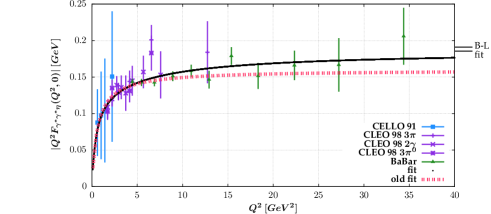
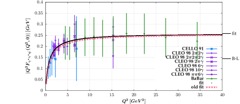
Figure 1: Transition form factors $\gamma^{*}\gamma P$ in the space-like region compared to the data.

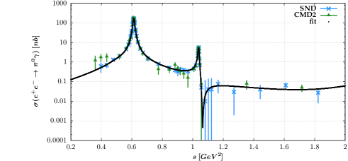
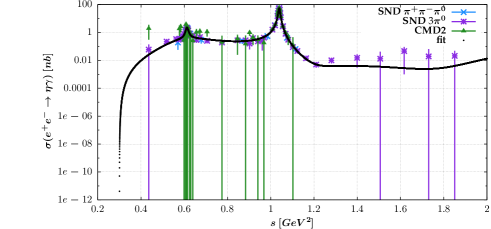
Figure 2: Experimental data for $\sigma(e^{+}e^{-}\to P\gamma)$ compared to the model predictions.

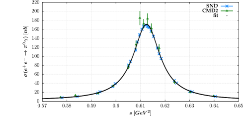
Figure 3: Experimental data for $\sigma(e^{+}e^{-}\to P\gamma)$ compared to the model predictions. The region of the $s$ has been limited to $\omega$ peak.

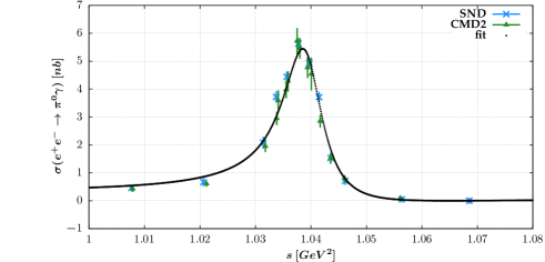
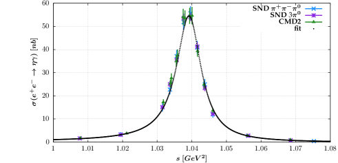
Figure 4: Experimental data for $\sigma(e^{+}e^{-}\to P\gamma)$ compared to the model predictions. The region of the $s$ has been limited to $\phi$ peak.

              

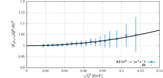
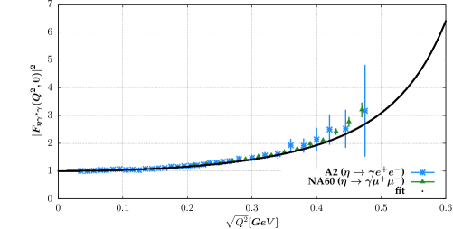
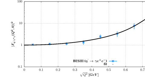
Figure 5: Transition form factors $\gamma^{*}\gamma P$ in the time-like region compared to the data.

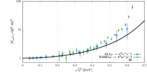
Figure 6: The form factor $\omega\pi^{0}\gamma$ in the time-like region compared to the data.

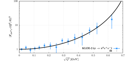
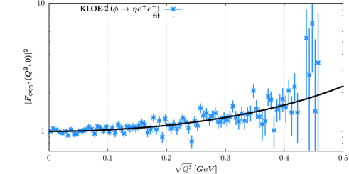
Figure 7: The form factor $\phi P\gamma$ in the time-like region compared to the data.

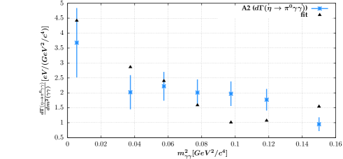
Figure 8: The differential partial width of the decay $\eta\to\pi^{0}\gamma\gamma$ compared to the data.

IV The asymptotics of the form factors and slopes of the form factors at the origin

The analytic form of the asymptotic behaviour of the form factors is analogous to the one obtained in Czyz et al. (2012) with the asymptotic limits changed. For completeness we report here the formulae, but skip the discussion as it should repeat the one presented in Czyz et al. (2012). They read

$$\kern-20.0ptF_{\gamma^{*}\gamma\pi^{0}}(t,0)=\sum^{n}_{i=1}\frac{4\sqrt{2}h_{V_{i}}f_{V_{i}}}{3f_{\pi}}\frac{1}{t}$$

$$\kern-10.0pt\bigg{(}M^{2}_{\rho_{i}}+F_{\omega_{i}}H_{\omega_{i}}M^{2}_{\omega_{i}}+A_{i}^{\pi^{0}}F_{\phi_{i}}M^{2}_{\phi_{i}}\bigg{)}+O\bigg{(}\frac{1}{t^{2}}\bigg{)}\,,$$ (40)

$$\kern-10.0ptF_{\gamma^{*}\gamma^{*}\pi^{0}}(t,t)=\sum^{n}_{i=1}\frac{4\sqrt{2}h_{V_{i}}f_{V_{i}}}{3f_{\pi}}\frac{1}{t^{2}}$$

$$\bigg{(}-2M^{2}_{\rho_{i}}M^{2}_{\omega_{i}}-(A_{i}^{\pi^{0}}F_{\phi_{i}}-A_{\phi\omega,i}^{\pi^{0}})M^{4}_{\phi_{i}}-2A_{\phi\omega,i}^{\pi^{0}}M^{2}_{\phi_{i}}M^{2}_{\omega_{i}}$$

$$-(F_{\omega_{i}}H_{\omega_{i}}-1-A_{\phi\omega,i}^{\pi^{0}})M^{4}_{\omega_{i}}\bigg{)}+O\bigg{(}\frac{1}{t^{3}}\bigg{)}\,,$$ (41)

$$\kern-30.0ptF_{\gamma^{*}\gamma\eta}(t,0)=\sum^{n}_{i=1}\frac{4\sqrt{2}h_{V_{i}}f_{V_{i}}}{3f_{\pi}}\frac{1}{t}$$

$$\bigg{(}3C_{q}M^{2}_{\rho_{i}}+\frac{1}{3}F_{\omega_{i}}C_{q}M^{2}_{\omega_{i}}-\frac{2\sqrt{2}}{3}C_{s}F_{\phi_{i}}M^{2}_{\phi_{i}}$$

$$+\big{(}\frac{5}{3}C_{q}-\frac{\sqrt{2}}{3}C_{s}\big{)}A_{i}^{\eta}F_{\phi_{i}}M^{2}_{\phi_{i}}\bigg{)}+O\bigg{(}\frac{1}{t^{2}}\bigg{)}\,,$$ (42)

$$\kern-25.0ptF_{\gamma^{*}\gamma^{*}\eta}(t,t)=\sum^{n}_{i=1}\frac{8\sqrt{2}h_{V_{i}}f_{V_{i}}}{f_{\pi}}\frac{1}{t^{2}}$$

$$\kern-10.0pt\bigg{(}-\frac{1}{2}C_{q}M^{4}_{\rho_{i}}-\frac{1}{18}F_{\omega_{i}}C_{q}M^{4}_{\omega_{i}}+A_{\phi\omega,i}^{\eta}M^{4}_{\omega_{i}}$$

$$+\frac{\sqrt{2}}{9}C_{s}F_{\phi_{i}}M^{4}_{\phi_{i}}-\frac{A_{i}^{\eta}F_{\phi_{i}}}{6}\big{(}\frac{5}{3}C_{q}-\frac{\sqrt{2}}{3}C_{s}\big{)}M^{4}_{\phi_{i}}$$

$$+A^{\eta}_{\phi\omega,i}M^{4}_{\phi_{i}}+2A^{\eta}_{\phi\omega,i}M^{2}_{\phi_{i}}M^{2}_{\omega_{i}}\bigg{)}+O\bigg{(}\frac{1}{t^{3}}\bigg{)}\,,$$ (43)

$$\kern-30.0ptF_{\gamma^{*}\gamma\eta^{{}^{\prime}}}(t,0)=\sum^{n}_{i=1}\frac{4\sqrt{2}h_{V_{i}}f_{V_{i}}}{3f_{\pi}}\frac{1}{t}$$

$$\bigg{(}3C_{q}^{{}^{\prime}}M^{2}_{\rho_{i}}+\frac{1}{3}F_{\omega_{i}}C_{q}^{{}^{\prime}}M^{2}_{\omega_{i}}+\frac{2\sqrt{2}}{3}C_{s}^{{}^{\prime}}F_{\phi_{i}}M^{2}_{\phi_{i}}$$

$$+\big{(}\frac{5}{3}C_{q}^{{}^{\prime}}+\frac{\sqrt{2}}{3}C_{s}^{{}^{\prime}}\big{)}A_{i}^{\eta^{{}^{\prime}}}F_{\phi_{i}}M^{2}_{\phi_{i}}\bigg{)}+O\bigg{(}\frac{1}{t^{2}}\bigg{)}\,,$$ (44)

$$\kern-20.0ptF_{\gamma^{*}\gamma^{*}\eta^{{}^{\prime}}}(t,t)=\sum^{n}_{i=1}\frac{-8\sqrt{2}h_{V_{i}}f_{V_{i}}}{f_{\pi}}\frac{1}{t^{2}}$$

$$\bigg{(}\frac{1}{2}C_{q}^{{}^{\prime}}M^{4}_{\rho_{i}}+\frac{1}{18}F_{\omega_{i}}C_{q}^{{}^{\prime}}M^{4}_{\omega_{i}}+\frac{\sqrt{2}}{9}C_{s}^{{}^{\prime}}F_{\phi_{i}}M^{4}_{\phi_{i}}$$

$$+\frac{A_{i}^{\eta^{{}^{\prime}}}F_{\phi_{i}}}{6}\big{(}\frac{5}{3}C_{q}^{{}^{\prime}}+\frac{\sqrt{2}}{3}C_{s}^{{}^{\prime}}\big{)}M^{4}_{\phi_{i}}\bigg{)}+O\bigg{(}\frac{1}{t^{3}}\bigg{)}\,.$$ (45)

The models are compared often by comparing the slopes of the form factors at the origin, which we denote as $a_{P}$. For the pseudoscalar transition form factors they are defined as:

$$a_{P}\equiv\frac{1}{F_{\gamma^{*}\gamma^{*}P}(0,0)}\frac{dF_{\gamma^{*}\gamma^{*}P}(t,0)}{dx}\bigg{|}_{t=0}$$ (46)

where $x\equiv\frac{t}{m^{2}_{P}}$. The model predictions for the model developed in this paper read:

$$a_{\pi^{0}} = \frac{16\sqrt{2}\pi^{2}m_{\pi^{0}}^{2}}{N_{c}}\sum^{3}_{i=1}h_{V_{i}}f_{V_{i}}$$ (47)

$$\bigg{(}\frac{1}{M^{2}_{\rho_{i}}}+F_{\omega_{i}}H_{\omega_{i}}\frac{1}{M^{2}_{\omega_{i}}}+A^{\pi^{0}}_{i}F_{\phi_{i}}\frac{1}{M^{2}_{\phi_{i}}}\bigg{)}$$

$$a_{\eta} = \frac{16\sqrt{2}\pi^{2}m_{\eta}^{2}}{N_{c}(\frac{5}{3}C_{q}-\frac{\sqrt{2}}{3}C_{s})}\sum^{3}_{i=1}h_{V_{i}}f_{V_{i}}$$ (48)

$$\bigg{(}3C_{q}\frac{1}{M^{2}_{\rho_{i}}}+\frac{1}{3}F_{\omega_{i}}C_{q}\frac{1}{M^{2}_{\omega_{i}}}-\frac{2\sqrt{2}}{3}C_{s}F_{\phi_{i}}\frac{1}{M^{2}_{\phi_{i}}}$$

$$+(\frac{5}{3}C_{q}-\frac{\sqrt{2}}{3}C_{s})A^{\eta}_{i}F_{\phi_{i}}\frac{1}{M^{2}_{\phi_{i}}}\bigg{)}$$

$$a_{\eta^{{}^{\prime}}} = \frac{16\sqrt{2}\pi^{2}m_{\eta^{`}}^{2}}{N_{c}(\frac{5}{3}C^{{}^{\prime}}_{q}+\frac{\sqrt{2}}{3}C^{{}^{\prime}}_{s})}\sum^{3}_{i=1}h_{V_{i}}f_{V_{i}}$$ (49)

$$\bigg{(}3C^{{}^{\prime}}_{q}\frac{1}{M^{2}_{\rho_{i}}}+\frac{1}{3}F_{\omega_{i}}C^{{}^{\prime}}_{q}\frac{1}{M^{2}_{\omega_{i}}}+\frac{2\sqrt{2}}{3}C^{{}^{\prime}}_{s}F_{\phi_{i}}\frac{1}{M^{2}_{\phi_{i}}}$$

$$+(\frac{5}{3}C^{{}^{\prime}}_{q}+\frac{\sqrt{2}}{3}C^{{}^{\prime}}_{s})A^{\eta^{{}^{\prime}}}_{i}F_{\phi_{i}}\frac{1}{M^{2}_{\phi_{i}}}\bigg{)}$$

The numerical comparison between predictions within different models and direct extractions from recent experiments is made in Table 3. The obtained results are in fair agreement with both.

Model	$a_{\pi^{0}}$	$a_{\eta}$	$a_{\eta^{{}^{\prime}}}$
fit 1	0.0298(3)	0.542(4)	1.357(9)
fit 2	0.0310(7)	0.536(11)	1.39(3)
Czyz et al. (2012)	0.02870(9)	0.521(2)	1.323(4)
Ametller et al. (1992)	0.0324	0.506	1.470
Hanhart et al. (2013)	-	0.62+0.06-0.03	-
Escribano et al. (2014)	-	$0.60(6)_{st}(3)_{sy}$	$1.30(15)_{st}(7)_{sy}$
Escribano et al. (2015)	-	$0.576(11)_{st}(4)_{sy}$	-
Escribano et al. (2016)	-	-	1.31(4)
CELLO Behrend et al. (1991)	0.0326(26)	0.428(63)	1.46(16)
SINDRUM-I Meijer Drees et al. (1992)	$0.026(24)_{st}(48)_{sy}$	-	-
Farzanpay et al. (1992)	$0.025(14)_{st}(26)_{sy}$	-	-
Mami Berghauser et al. (2011)	-	$0.576(105)_{st}(39)_{sy}$	-
NA60 Usai (2011)	-	$0.585(18)_{st}(13)_{sy}$	-
NA62 Lazzeroni et al. (2017)	$0.0368(51)_{st}(25)_{sy}$	-	-

Table 3: The slope parameter $a_{P}$ (Eq.(46)) compared to other model predictions and experimental data.

V Pseudoscalar contributions to $a_{\mu}$

Model	$a_{\mu}^{\pi^{0}}$	$a_{\mu}^{\eta}$	$a_{\mu}^{\eta^{{}^{\prime}}}$	$a_{\mu}^{P}$
fit 1	$58.80\pm 0.27$	$13.56\pm 0.10$	$12.97\pm 0.09$	$85.32\pm 0.30$
fit 2	$56.96\pm 0.94$	$13.35\pm 0.45$	$12.55\pm 0.48$	$82.85\pm 1.15$
fit 3	$59.07\pm 0.17$	$13.52\pm 0.09$	$12.96\pm 0.09$	$85.55\pm 0.22$
fit 4	$57.79\pm 0.90$	$13.31\pm 0.19$	$12.31\pm 0.21$	$83.41\pm 0.94$
Hayakawa and Kinoshita (1998)	$57.4\pm 6.0$	$13.4\pm 1.6$	$11.9\pm 1.4$	$82.7\pm 6.4$
Knecht and Nyffeler (2002)	$58\pm 10$	$13\pm 1$	$12\pm 1$	$83\pm 12$
Bijnens et al. (2002)	-	-	-	$85\pm 13$
Melnikov and Vainshtein (2004)	$76.5\pm 6.5$	$18\pm 1.4$	$18\pm 1.5$	$114\pm 10$
Dorokhov and Broniowski (2008)	$62.7-66.8$	-	-	-
Nyffeler (2009); Jegerlehner and Nyffeler (2009)	$72\pm 12$	$14.5\pm 4.8$	$12.5\pm 4.2$	$99\pm 16$
Kampf and Novotny (2011)	$68.8\pm 1.2$	-	-	-
Roig et al. (2014)	$66.6\pm 2.1$	$20.4\pm 4.4$	$17.7\pm 2.3$	$104.7\pm 5.4$
Gérardin et al. (2016)	$65.0\pm 8.3$	-	-	-

Table 4: Pseudoscalar-exchange contribution to the $a_{\mu}^{HLBL,PS}\times 10^{11}$ ($PS=\pi^{0},\eta,\eta^{{}^{\prime}}$).

Within the model described in the previous sections we calculate the contributions from the pseudoscalar mesons $\pi^{0},\eta$ and $\eta^{\prime}$ to the muon anomalous magnetic moment $a_{\mu}$. The formula Eq.(155) of Jegerlehner and Nyffeler (2009) was used with the form factors developed in this paper Eqs.(14-16). The variables spanned from zero to infinity were mapped on the intervals $(0,1)$ and the integrals were performed using the Monte Carlo method. For a cross check of the numerical method and the implementation we have recovered values from Table 7 of Jegerlehner and Nyffeler (2009) using the model(s) presented there. The results are presented in Table 4 for both fits and compared with previous calculations. For the error evaluation we have used the covariance matrix calculated by Minuit from CERNLIB. The derivatives of the $a_{\mu}$ in respect to the fitting parameters were calculated numerically, using the Monte Carlo method to obtain the necessary integrals. The error of the sum of all the contributions from pseudoscalars was calculated separately as an error on the function being the sum of the free contributions. As one can observe the obtained results are consistent with most of other models. The biggest differences, not contained in the error bars, are observed with calculations presented in Melnikov and Vainshtein (2004); Kampf and Novotny (2011); Roig et al. (2014). The much smaller errors of our calculations, as compared to other results, are only parametric and do not cover the model dependence. Yet, it has to be stressed that the model is able to describe well all the existent data on the form factors both in the space-like and time-like regions. To cover the model dependence within the class of models we consider here we added two values of $a_{\mu}$ (fit 4 and fit 5). In the models 4 and 5 we have excluded from the fit the cross sections of the reactions $e^{+}e^{-}\to\eta\gamma$ and $e^{+}e^{-}\to\eta^{\prime}\gamma$ measured by BaBar Aubert et al. (2006) at very high energy compared to other data points. The fits were performed with parameters $A_{3}^{P}$ set to zero and with fixed or fitted mixing parameters similarly to fits 1 and 2. The $e^{+}e^{-}\to\eta^{\prime}\gamma$ cross section calculated at the BaBar energy point is off the measured value by about 5 standard deviations. Also the predicted $e^{+}e^{-}\to\pi^{0}\gamma$ cross section at $s=112\ {\rm GeV}^{2}$ is different for both fits. However, as expected from the analysis in Nyffeler (2016), the values of the pseudoscalar form factors at large invariant masses are much less important than the behaviour in the range up to about 1 GeV for the calculation of $a_{\mu}$. Thus the very close results for $a_{\mu}$ coming from all the fits are not surprising. The range of the predicted values of $a_{\mu}$ within the class of models we examined is thus $79.4\times 10^{11}<a_{\mu}^{P}<86.23\times 10^{-11}$, if we take conservatively $3\sigma$ errors, and the predicted value of $a_{\mu}$ is $(82.8\pm 3.4)\times 10^{-11}$.

VI The implementation of the model in Ekhara and Phokhara generators

The new transition pseudoscalar form factors were implemented in the event generator EKHARA Czyz and Ivashyn (2011); Czyz and Nowak-Kubat (2006). As one can see from Figure 1 the difference of the form factors from this paper as compared to the old model Czyz et al. (2012), for the configuration, where one of the invariant is equal to zero, is not big. Yet, the experiments never have the second invariant mass equal to zero and the events are collected with a cut resulting from the cuts on the observed particles. The influence of this effect on the experimental side is a part of the systematic error. On the theory side it is model dependent, with the part which is different from zero only when both photon virtualities are different from zero never tested directly by any experiment in the space-like region. The difference of the predictions of the influence of the second virtuality between the old and the new model is shown in Figure 9. We plot there the relative difference of the differential cross sections calculated with the complete form factors (full) and the case where one of the invariants was set to zero (approx) as a function of the second invariant $Q^{2}=-(q-p)^{2}$. $q$ is the four-vector of the final positron and $p$ is the four-vector of the initial positron. We limit the invariant mass squared of the first virtual photon ($Q_{1}^{2}=-(q^{\prime}-p^{\prime})^{2}$, where $q^{\prime}$ is the four-vector of the final electron and $p^{\prime}$ is the four-vector of the initial electron) to $Q_{1}^{2}\leq 0.18$ GeV for $\pi^{0}$ and to $Q_{1}^{2}\leq 0.38$ for $\eta$ and $\eta^{\prime}$. As one can see the corrections coming from the second invariant are by no means negligible, and their size exhibits the model dependence. In the plot the form factors of the ’fit 2’ were used. For the ’fit 1’ they look similar.

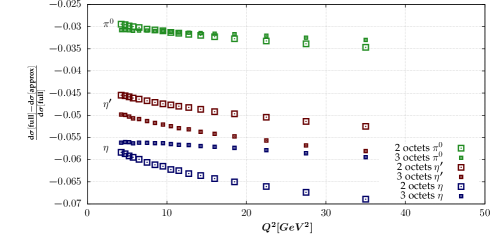
Figure 9: The relative difference of differential cross sections calculated with $F_{\gamma^{*}\gamma^{*}P}(-Q^{2},q_{1}^{2})$ (full) and $F_{\gamma^{*}\gamma^{*}P}(-Q^{2},0)$ (approx). See text for details.

Having the model of the pseudoscalar transition form factors valid also in the time-like region we are able to simulate the cross sections of the reactions $e^{+}e^{-}\to P\gamma$. This is done within the Phokhara Monte Carlo generator Rodrigo et al. (2002) framework. It is an upgrade of the version 9.2 Czyz et al. (2016) and will be available from the web page (http://ific.uv.es/$\sim$rodrigo/phokhara/) as release 9.3. Both options with the fit 1 and the fit 2 parameters are implemented. The next to leading order initial state radiative corrections were included basing on the approach described in Czyz et al. (2013). The virtual and the soft initial state corrections are universal and are exactly the same as in Czyz et al. (2013), thus we do not repeat here the formulae. The matrix element describing the reaction $e^{+}e^{-}\to\pi^{0}\gamma\gamma$ was written as a product of leptonic and hadronic current:

$$\mathcal{M}[e^{+}(p_{1})e^{-}(p_{2})\to\pi^{0}(q_{1})\gamma(k_{1})\gamma(k_{2})]$$

$$=L^{\nu}(k_{1})H_{\nu}(k_{2})+(k_{1}\leftrightarrow k_{2}),$$ (50)

where

$$H_{\nu}(k_{2})=e^{2}\epsilon_{\mu\nu\alpha\beta}q_{1}^{\mu}k_{2}^{\alpha}\epsilon_{2}^{\beta}F_{\gamma^{*}\gamma^{*}P}\big{(}(q_{1}+k_{2})^{2},0\big{)}$$ (51)

and

$$L^{\nu}(k_{1}) = \frac{ie^{2}}{2p_{2}\cdot k_{1}}\bar{v}(p_{1})\gamma^{\nu}\Big{(}2\epsilon_{1}p_{1}-k_{1}/\hskip 1.99997pt\epsilon_{1}/\hskip 1.99997pt\Big{)}u(p_{2})$$

$$+\frac{ie^{2}}{2p_{1}\cdot k_{1}}\bar{v}(p_{1})\Big{(}\epsilon_{1}/\hskip 1.99997ptk_{1}/\hskip 1.99997pt-2\epsilon_{1}p_{1}\Big{)}\gamma^{\nu}u(p_{2}),$$

with $\epsilon_{i},i=1,2$ being a polarization vector of the photon with the four momentum $k_{i}$.

The effect of radiative corrections is shown in Figure 10. The plots were obtained using fit 2 parameters accepting the events with the pseudoscalar particle and one of the photons with an energy bigger than 0.5 GeV being observed within the angular range between 20 and 160 degrees. The radiative corrections are big due to the fact that the pseudoscalar transition form factor is falling fast at high values of the virtual photon mass. At LO (leading order) the form factor is calculated at $s$, while in the two photon amplitude it is calculated at much smaller invariants $Q_{1}^{2}=(q_{1}+k_{1})^{2}$, or $Q_{2}^{2}=(q_{1}+k_{2})^{2}$ resulting from the hard photon emission.

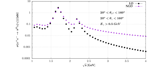
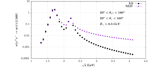
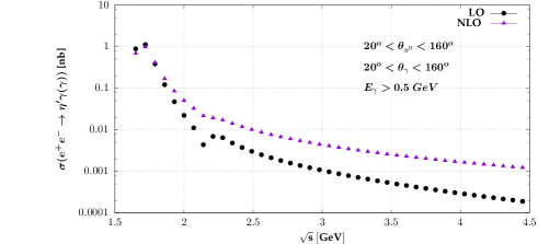
Figure 10: Comparison between LO and NLO cross sections. See text for details.

VII Conclusions

We model the Lagrangians $\mathcal{L}_{\gamma\gamma\mathcal{P}}$, $\mathcal{L}_{\gamma V}$, $\mathcal{L}_{V\gamma P}$ and $\mathcal{L}_{VVP}$ within the resonance chiral symmetric theory with the SU(3) breaking. Two model versions with 22(17) couplings of the model are fitted to 536 experimental data points resulting in $\chi^{2}=415(454)$. Within the developed models we predict the light-by-light contributions to the muon anomalous magnetic moment $a_{\mu}^{P}=(82.8\pm 3.4)\times 10^{-11}$. The error covers also the model dependence within the class of models considered in this paper. The model was implemented into the Monte Carlo event generator Ekhara to simulate the reactions $e^{+}e^{-}\to e^{+}e^{-}P$, ($P=\pi^{0},\ \eta,\ \eta^{\prime}$) and into the Monte Carlo event generator Phokhara to simulate the reactions $e^{+}e^{-}\to P\gamma(\gamma)$ at the next-to-leading order.

References

Actis et al. (2010)
S. Actis et al.
(Working Group on Radiative Corrections and Monte
Carlo Generators for Low Energies), Eur. Phys. J.
C66, 585 (2010),
eprint 0912.0749.
Bennett et al. (2006)
G. W. Bennett
et al. (Muon g-2),
Phys. Rev. D73,
072003 (2006), eprint hep-ex/0602035.
Hagiwara et al. (2007)
K. Hagiwara,
A. D. Martin,
D. Nomura, and
T. Teubner,
Phys. Lett. B649,
173 (2007), eprint hep-ph/0611102.
Davier et al. (2011)
M. Davier,
A. Hoecker,
B. Malaescu, and
Z. Zhang,
Eur. Phys. J. C71,
1515 (2011), [Erratum: Eur.
Phys. J.C72,1874(2012)], eprint 1010.4180.
Benayoun et al. (2015)
M. Benayoun,
P. David,
L. DelBuono, and
F. Jegerlehner,
Eur. Phys. J. C75,
613 (2015), eprint 1507.02943.
Hagiwara et al. (2017)
K. Hagiwara,
A. Keshavarzi,
A. D. Martin,
D. Nomura, and
T. Teubner,
Nucl. Part. Phys. Proc.
287-288, 33
(2017).
Stefanis et al. (2013)
N. G. Stefanis,
A. P. Bakulev,
S. V. Mikhailov,
and A. V.
Pimikov, Phys. Rev.
D87, 094025
(2013), eprint 1202.1781.
Noguera and Vento (2012)
S. Noguera and
V. Vento,
Eur. Phys. J. A48,
143 (2012), eprint 1205.4598.
Wu et al. (2013)
X.-G. Wu,
T. Huang, and
T. Zhong,
Chin. Phys. C37,
063105 (2013), eprint 1206.0466.
Klopot et al. (2013)
Y. Klopot,
A. Oganesian,
and O. Teryaev,
Phys. Rev. D87,
036013 (2013), [Erratum:
Phys. Rev.D88,no.5,059902(2013)], eprint 1211.0874.
Geng and Lih (2012)
C.-Q. Geng and
C.-C. Lih,
Phys. Rev. C86,
038201 (2012), [Erratum:
Phys. Rev.C87,no.3,039901(2013)], eprint 1209.0174.
Dumm et al. (2014)
D. G. Dumm,
S. Noguera,
N. N. Scoccola,
and S. Scopetta,
Phys. Rev. D89,
054031 (2014), eprint 1311.3595.
de Melo et al. (2014)
J. P. B. C. de Melo,
B. El-Bennich,
and
T. Frederico,
Few Body Syst. 55,
373 (2014), eprint 1312.6133.
Li et al. (2014)
H.-N. Li,
Y.-L. Shen, and
Y.-M. Wang,
JHEP 01, 004
(2014), eprint 1310.3672.