The Steklov Problem on Rectangles and Cuboids

Abstract

This paper is a brief account of the Steklov eigenvalue problem on a 2-dimensional rectangular domain, and then on a 3-dimensional rectangular box. It is divided into four sections. Section 1 relies heavily on real analytic methods to show the existence of an eigenfunction class which always produces the first non-trivial Steklov eigenvalue on a rectangle. Section 2 lists all possible Steklov eigenfunctions on a cuboid. The very brief section 3 gives the 3-dimensional analogue of the analytic results in Section 1. The analogue is given as conjecture, but is expected to derivate from standard (albeit tedious) real analysis methods, should one wish to expound on these calculations. Section 4 deals with the special cases of the square and the cube.

1 Analysis of the 1st Steklov eigenspace on the rectangle

Consider the rectangle defined on $[-1,1]\times[-a,a]$, where $a\leq 1$. One can classify the Steklov eigenfunctions on this domain into 4 parity classes (Auchmuty $\&$ Cho, 2014). Generally, each parity class has two eigenfunctions, but for the case of the square $(a=1)$, there is an additional eigenfunction $s(x,y)=xy$ in Class II, whose eigenvalue is simple and equal to $1$.
One can consider the smallest nontrivial eigenvalue $\sigma_{1}$, and ask: Among all rectangular domains with constant perimeter, which domains maximize the first Steklov eigenvalue, $\sigma_{1}$?
One may normalize the eigenvalue $\sigma_{1}$ by multiplying with the perimeter of the domain, $L=4(1+a)$. The product, $\sigma_{1}L$, is an invariant with respect to a scaling of the domain.
That is, one can define an equivalence relation between similar rectangles, with rectangles in the same equivalence class having the same first Steklov invariant. We identify any rectangle with a rectangle defined $[-1,1]\times[-a,a]$, where $a\leq 1$, so that we may restrict our analysis to such rectangles. Since similar rectangles have the same Steklov invariants, the question then becomes: Among all values of $a\in(0,1]$, which maximizes $4\sigma_{1}(1+a)$?
We show that $a=1$ does.
As mentioned above, we consider the eigenfunctions by parity class. In the table below, we only need to consider positive $\nu$.

Class	Eigenfunction	Determining Equation	Eigenvalue $\sigma$
I(i)	cosh$(\nu x)$cos$(\nu y)$,	tan$(\nu a)+$tanh$(\nu)=0$	$\nu$tanh$(\nu)$
I(ii)	cos$(\nu x)$cosh$(\nu y)$	tan$(\nu)+$tanh$(\nu a)=0$	$\nu$tanh$(\nu a)$
II(i)	sinh$(\nu x)$sin$(\nu y)$,	tan$(\nu a)=$tanh$(\nu)$	$\nu$coth$(\nu)$
II(ii)	sin$(\nu x)$sinh$(\nu y)$	tan$(\nu)=$tanh$(\nu a)$	$\nu$coth$(\nu a)$
III(i)	cosh$(\nu x)$sin$(\nu y)$,	tan$(\nu a)=$coth$(\nu)$	$\nu$tanh$(\nu)$
III(ii)	cos$(\nu x)$sinh$(\nu y)$	tan$(\nu)+$coth$(\nu a)=0$	$\nu$coth$(\nu a)$
IV(i)	sinh$(\nu x)$cos$(\nu y)$,	tan$(\nu a)+$coth$(\nu)=0$	$\nu$coth$(\nu)$
IV(ii)	sin$(\nu x)$cosh$(\nu y)$	tan$(\nu)=$coth$(\nu a)$	$\nu$tanh$(\nu a)$

Table 1: The eigenfunctions fall into eight classes.

(We have omitted $s(x,y)=xy$, which only arises when $a=1$.)

Then, for instance, the 1st Steklov eigenfunction from class IV(ii) has value $\nu$ given by the 1st positive solution of tan$\nu=$coth$(\nu a)$. Of course, for given $a$, minimizing $\nu$ is equivalent to minimizing $\nu$tanh$(\nu a)$. In fact, we have the following simple lemma.

Lemma 1.1.

For given $a\in(0,1]$, the maps $\nu\mapsto\nu$tanh$(\nu a)$ and $\nu\mapsto\nu$coth$(\nu a)$ are increasing on $\nu\in(0,\infty)$ (Auchmuty $\&$ Cho, 2014).

We claim that the 1st nontrivial Steklov eigenvalue for a rectangle always comes from class IV(ii).

By considering intersections of graphs (see Figure 1 of Girouard $\&$ Polterovich, 2014), it is trivial that III(i) is a better minimizer of $\nu$ – and therefore $\sigma$ – than I(i). Likewise IV(ii) is a better minimizer of $\nu$ than I(ii), II(ii), and III(ii). Since tanh$(\nu a)<$ coth$(\nu a)$, we have that IV(ii) gives the smallest value of $\sigma$ compared with I(ii), II(ii), and III(ii).

It remains to compare II(i), III(i), IV(ii).

Claim 1.

Fix $a\in(0,1]$. For a rectangle on $[-1,1]\times[-a,a]$, let the candidate for the 1st Steklov eigenvalue from class II(i) be $\sigma_{1}^{II(i)}$, and that from class III(i) be $\sigma_{1}^{III(i)}$. Then $\sigma_{1}^{III(i)}<\sigma_{1}^{II(i)}$.

Proof.

We want to show that III(i) is a better minimizer of $\sigma_{1}$ than II(i). For II(i), an eigenvalue $\sigma$ is given by an intersection of the graphs $\sigma=\nu$coth$(\nu)$ and $\sigma=\nu$cot$(\nu a)$. For III(i), an eigenvalue $\sigma$ is given by an intersection of the graphs $\sigma=\nu$tanh$(\nu)$ and $\sigma=\nu$cot$(\nu a)$.

Naturally, in either case, the candidate for $\sigma_{1}$ is the intersection which has the lowest height.

We show that the candidate for $\sigma_{1}$ is smaller in the case of III(i).

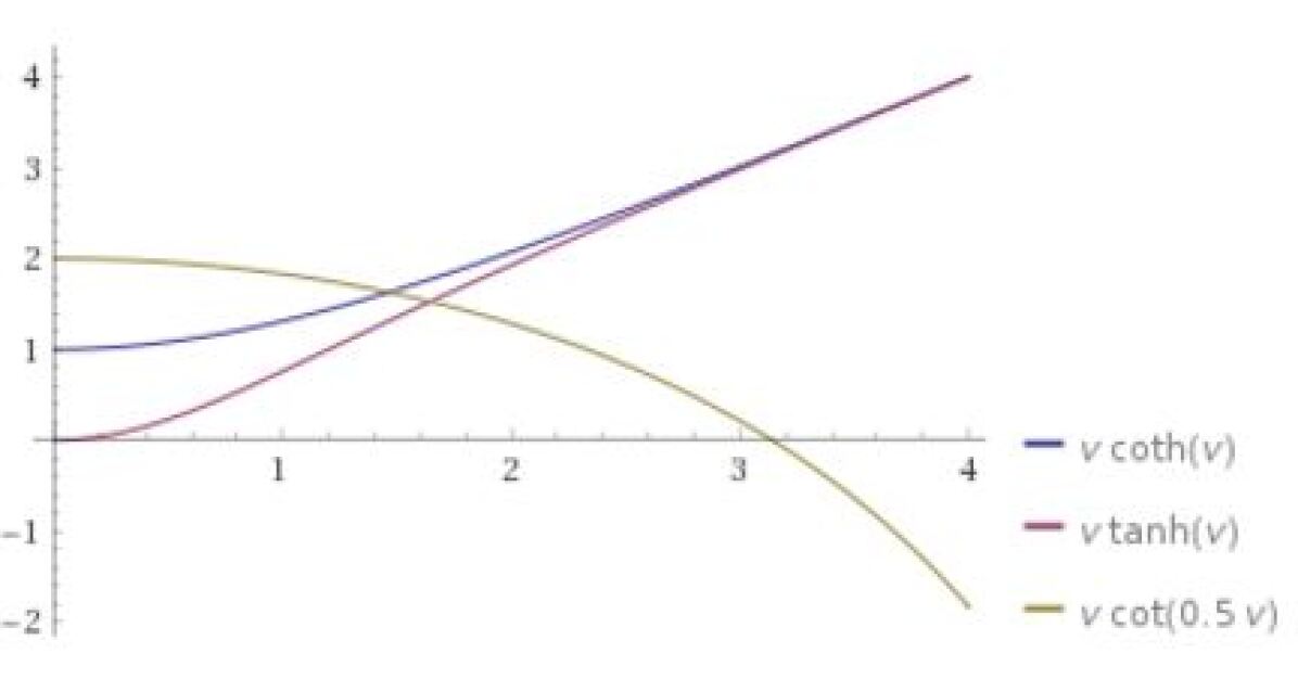
Figure 1: The graphs for $a=0.5$.

In each case, the lowest intersection must also be the intersection nearest to to the $\sigma$-axis, by Lemma 1.1. Hence we need only consider the graphs on $0<\nu<\nu_{0}$ where $\nu_{0}=\frac{\pi}{2a}$. Figure 1 compares the lowest intersections for case III(i) and II(i). By the intermediate value theorem, there exists a candidate for $\sigma_{1}$ in $0<\nu<\nu_{0}$ for both cases III(i) and II(i). By the strict monotonicity of the graphs on this interval, these candidates are unique. Finally, the candidate from class III(i) has a lower height than the candidate from class II(i), because the graph of $\sigma=\nu$cot$(\nu a)$ is strictly decreasing on $0<\nu<\nu_{0}$. Otherwise we would derive a contradiction by the mean value theorem.

∎

Claim 2.

Fix $a\in(0,1]$. For a rectangle on $[-1,1]\times[-a,a]$, let the candidate for the 1st Steklov eigenvalue from class III(i) be $\sigma_{1}^{III(i)}$, and that from class IV(ii) be $\sigma_{1}^{IV(ii)}$. Then $\sigma_{1}^{IV(ii)}\leq\sigma_{1}^{III(i)}$, with equality iff $a=1$.

Proof.

Similar to before, we want to show that IV(ii) is a better minimizer of $\sigma_{1}$ than III(i). For III(i), an eigenvalue $\sigma$ is given by an intersection of the graphs $\sigma=\nu$tanh$(\nu)$ and $\sigma=\nu$cot$(\nu a)$. For IV(ii), an eigenvalue $\sigma$ is given by an intersection of the graphs $\sigma=\nu$coth$(\nu a)$ and $\sigma=\nu$cot$(\nu)$.

We show that the candidate for $\sigma_{1}$ is smaller in the case of IV(ii).

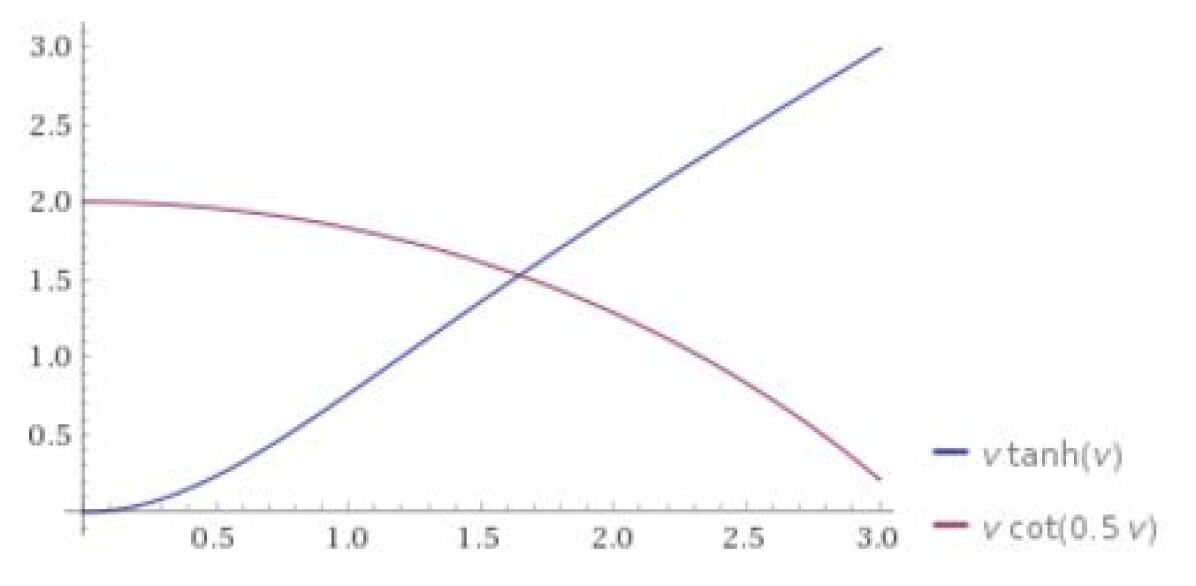
Figure 2: The candidate for $\sigma_{1}$ of Class III(i), in the case $a=0.5$.

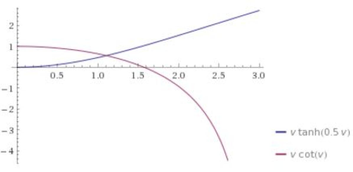
Figure 3: The candidate for $\sigma_{1}$ of Class IV(ii), in the case $a=0.5$.

In each case, the lowest intersection must also be the intersection nearest to to the $\sigma$-axis, by $(*)$. Hence we need only consider the graphs on $0<\nu<\nu_{0}$ where $\nu_{0}=\frac{\pi}{2a}$. Figures 2 and 3 give the lowest intersection for class III(i) and class IV(ii) respectively. These intersections can be shown to exist in $0<\nu<\nu_{0}$ by the intermediate value theorem. (A sample calculation for this is done explicitly in the proof of Claim 3.) Since it is clear that both graphs in Figure 3 are lower than the respective graphs in Figure 2, we can conclude that $\sigma_{1}^{IV(ii)}<\sigma_{1}^{III(i)}$.

∎

We have just shown that the 1st Steklov invariant on a given rectangle is always given by eigenfunction IV(ii)! Moreover, for $a\neq 1$, this is the only eigenfunction in the 1st eigenspace, because $\sigma_{1}^{IV(ii)}$ is strictly smaller than any other eigenvalue. Let us state this as a theorem.

Theorem 1.2.

On any rectangular domain that is not a square, the 1st Steklov eigenspace has basis $\{$sin$(\nu x)$cosh$(\nu y)$$\}$.

Below is a graph of this invariant against the length $a\in(0,1]$.

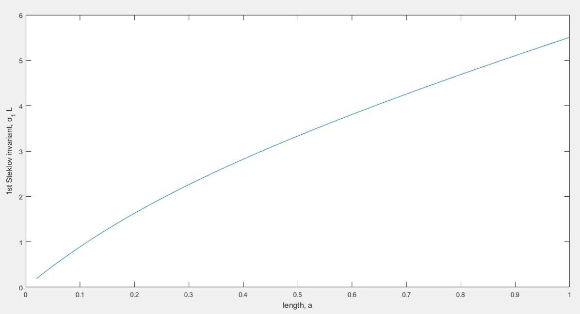
Figure 4: The 1st Steklov invariant for a rectangle on $[-1,1]\times[-a,a]$.

For completeness, we also plot the invariant given by each of the 8 eigenfunctions against $a$ in Figure 5.

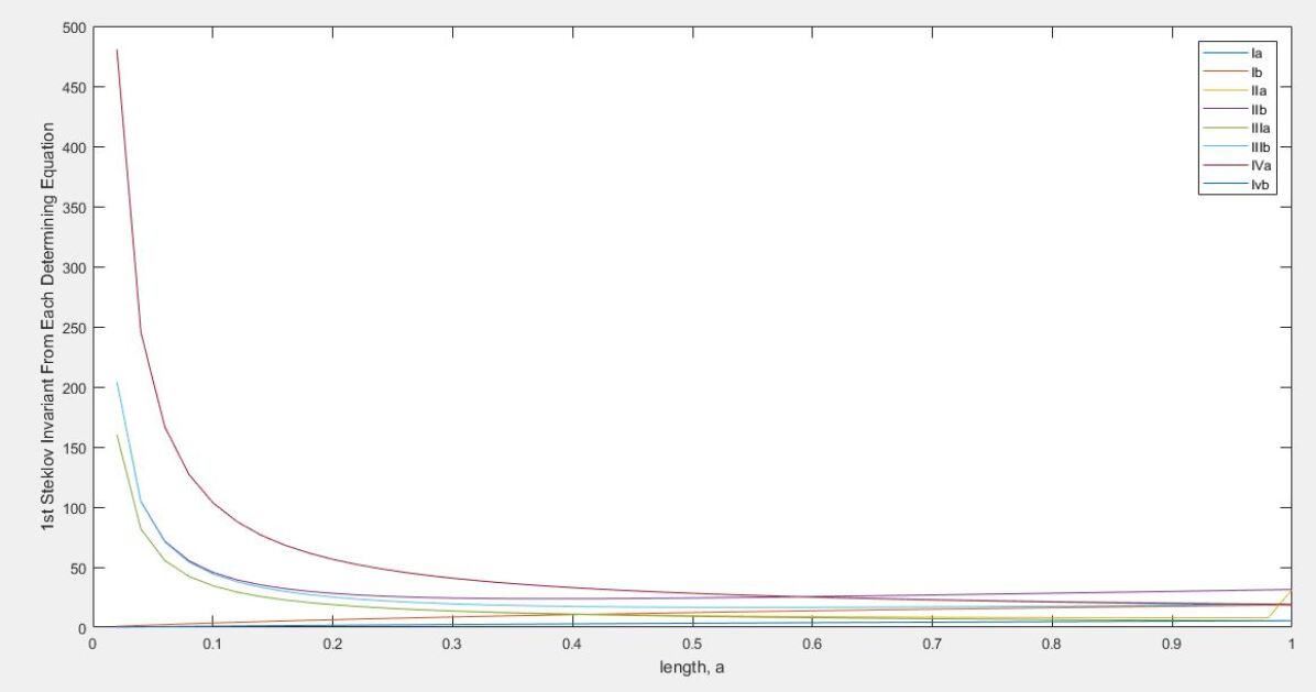
Figure 5: The 1st Steklov invariant for each of 8 determining equations.

The lowest graph in Figure 5 is, of course, the same graph as in Figure 4. Figure 4 suggests that $a=1$ maximizes the 1st Steklov invariant. In fact, we now show that the graph is differentiable, increasing with $a$, and tends to the origin (in the first quadrant).

Claim 3.

The graph in Figure 4 is differentiable on $a\in(0,1)$.

Proof.

Fix $a\in(0,1)$. Define $k_{a}:(0,\frac{\pi}{2})\to\mathbb{R}$, $k_{a}(\nu)=\nu$cot$(\nu)-\nu$tanh$(\nu a)$. Since $\lim_{\nu\downarrow 0}k_{a}(\nu)=1>0$ and $\lim_{\nu\uparrow\frac{\pi}{2}}k_{a}(\nu)=-\frac{\pi}{2}\text{tanh}(\frac{\pi}{2}a)<0$, the intermediate value theorem guarantees some root $\nu_{1}^{IV(ii)}\in(0,\frac{\pi}{2})$. That is, cot$(\nu_{1}^{IV(ii)})-$tanh$(\nu_{1}^{IV(ii)}a)=0$. In fact, $\nu_{1}^{IV(ii)}$ is unique since $k_{a}$ is strictly decreasing. (Clearly $\sigma_{1}^{IV(ii)}=\nu_{1}^{IV(ii)}$tanh$(\nu_{1}^{IV(ii)}a)$.) The above allows me to define $h:\mathbb{R}\times(0,\frac{\pi}{2})\to\mathbb{R}$, $h(a,\nu)=k_{a}(\nu)$. Next, we show that $\nu$ is a differentiable function of $a\in(0,1)$ by applying the implicit function theorem to $h$. At each root $(a,\nu_{1}^{IV(ii)})$ of $h$, we check that $h_{\nu}\neq 0$:

$$h_{\nu}(\ (a,\nu_{1}^{IV(ii)})\ ) =-\text{tanh}(\nu_{1}^{IV(ii)}a)-\nu_{1}^{IV(ii)}a\text{sech}^{2}(\nu_{1}^{IV(ii)}a)+\text{cot}(\nu_{1}^{IV(ii)})-\nu_{1}^{IV(ii)}\text{cosec}^{2}(\nu_{1}^{IV(ii)})$$

$$=-\nu_{1}^{IV(ii)}a\text{sech}^{2}(\nu_{1}^{IV(ii)}a)-\nu_{1}^{IV(ii)}\text{cosec}^{2}(\nu_{1}^{IV(ii)})$$

$$<0.$$

Therefore the implicit function theorem ensures that $\nu$ is locally a differentiable function of $a$ for each $a\in(0,1)$, and hence globally differentiable on $(0,1)$. It is also continuous on $[0,1]$. The composition $\sigma=\nu$tanh$(\nu a)$ is therefore a differentiable function of $a$. ∎

Claim 4.

The graph in Figure 4 is strictly increasing on $(0,1]\ni a$. Moreover, $\sigma\downarrow 0$ as $a\downarrow 0$.

Proof.

Consider again Figure 3, which displays (for the special case $a=0.5$) the intersection of $\sigma=\nu$tanh$(\nu a)$ with $\sigma=\nu$cot$(\nu)$. Clearly as $a\downarrow 0$, the intersection height decreases (continuously!) to $0$. Moreover, for $a_{1}<a_{2}$, we have $\sigma_{1}<\sigma_{2}$. ∎

(Alternatively, by examining the Rayleigh quotient, one can see easily that $\sigma\downarrow 0$ as $a\downarrow 0$.)

2 Finding Steklov eigenfunctions on a cuboid

Now we move to the 3D case. The notation here is such that $(a,b,c)$ give the dimensions of a cube, but similarly to the 2D case, we may let $c=1$ be the longest side without loss of generality.

Let us consider a cuboid on $[-a,a]\times[-b,b]\times[-c,c]$. we use separation of variables to solve Laplace’s equation with a Steklov condition on the faces of the cuboid. This treatment will assume the completeness of the set of eigenfunctions obtained by separation of variables. For the 2D case, completeness can be shown using ’sloshing’ methods (see Girouard and Polterovich, 2014).
By symmetry, we only need to consider eigenfunctions which are odd or even in $x$, $y$, and $z$. This gives 8 parity classes of eigenfunctions. In the tables below, we need only consider $\lambda_{i}>0$.

1. CLASS 000: Even in $x$, $y$, $z$.

$$Eigenfunction Eigenvalue$$

  s(x,y,z) $$&= \sigma =0$$

$$s(x,y,z) =\text{cos}(\sqrt{\lambda_{1}^{2}+\lambda_{2}^{2}}x)\text{cosh}(\lambda_{1}y)\text{cosh}(\lambda_{2}z) \sigma =\lambda_{1}\text{tanh}(\lambda_{1}b)=\lambda_{2}\text{tanh}(\lambda_{2}c)=-\sqrt{\lambda_{1}^{2}+\lambda_{2}^{2}}\text{tan}(\sqrt{\lambda_{1}^{2}+\lambda_{2}^{2}}a)$$

$$s(x,y,z) =\text{cosh}(\lambda_{1}x)\text{cos}(\sqrt{\lambda_{1}^{2}+\lambda_{2}^{2}}y)\text{cosh}(\lambda_{2}z) \sigma =\lambda_{1}\text{tanh}(\lambda_{1}a)=\lambda_{2}\text{tanh}(\lambda_{2}c)=-\sqrt{\lambda_{1}^{2}+\lambda_{2}^{2}}\text{tan}(\sqrt{\lambda_{1}^{2}+\lambda_{2}^{2}}b)$$

$$s(x,y,z) =\text{cosh}(\lambda_{1}x)\text{cosh}(\lambda_{2}y)\text{cos}(\sqrt{\lambda_{1}^{2}+\lambda_{2}^{2}}z) \sigma =\lambda_{1}\text{tanh}(\lambda_{1}a)=\lambda_{2}\text{tanh}(\lambda_{2}b)=-\sqrt{\lambda_{1}^{2}+\lambda_{2}^{2}}\text{tan}(\sqrt{\lambda_{1}^{2}+\lambda_{2}^{2}}c)$$

$$s(x,y,z) =\text{cosh}(\sqrt{\lambda_{1}^{2}+\lambda_{2}^{2}}x)\text{cos}(\lambda_{1}y)\text{cos}(\lambda_{2}z) \sigma =-\lambda_{1}\text{tan}(\lambda_{1}b)=-\lambda_{2}\text{tan}(\lambda_{2}c)=\sqrt{\lambda_{1}^{2}+\lambda_{2}^{2}}\text{tanh}(\sqrt{\lambda_{1}^{2}+\lambda_{2}^{2}}a)$$

$$s(x,y,z) =\text{cos}(\lambda_{1}x)\text{cosh}(\sqrt{\lambda_{1}^{2}+\lambda_{2}^{2}}y)\text{cos}(\lambda_{2}z) \sigma =-\lambda_{1}\text{tan}(\lambda_{1}a)=-\lambda_{2}\text{tan}(\lambda_{2}c)=\sqrt{\lambda_{1}^{2}+\lambda_{2}^{2}}\text{tanh}(\sqrt{\lambda_{1}^{2}+\lambda_{2}^{2}}b)$$

$$s(x,y,z) =\text{cos}(\lambda_{1}x)\text{cos}(\lambda_{2}y)\text{cosh}(\sqrt{\lambda_{1}^{2}+\lambda_{2}^{2}}z) \sigma =-\lambda_{1}\text{tan}(\lambda_{1}b)=-\lambda_{2}\text{tan}(\lambda_{2}a)=\sqrt{\lambda_{1}^{2}+\lambda_{2}^{2}}\text{tanh}(\sqrt{\lambda_{1}^{2}+\lambda_{2}^{2}}c)$$

2. CLASS 001: Even in $x$, $y$, Odd in $z$.

$$Eigenfunction Eigenvalue$$

  s(x,y,z) $$&=\text{cos}(\sqrt{\lambda_{1}^{2}+\lambda_{2}^{2}}x)\text{cosh}(\lambda_{1}y)\text{sinh}(\lambda_{2}z \sigma =\lambda_{1}\text{tanh}(\lambda_{1}b)=\lambda_{2}\text{coth}(\lambda_{2}c)=-\sqrt{\lambda_{1}^{2}+\lambda_{2}^{2}}\text{tan}(\sqrt{\lambda_{1}^{2}+\lambda_{2}^{2}}a)$$

$$s(x,y,z) =\text{cosh}(\lambda_{1}x)\text{cos}(\sqrt{\lambda_{1}^{2}+\lambda_{2}^{2}}y)\text{sinh}(\lambda_{2}z) \sigma =\lambda_{1}\text{tanh}(\lambda_{1}a)=\lambda_{2}\text{coth}(\lambda_{2}c)=-\sqrt{\lambda_{1}^{2}+\lambda_{2}^{2}}\text{tan}(\sqrt{\lambda_{1}^{2}+\lambda_{2}^{2}}b)$$

$$s(x,y,z) =\text{cosh}(\lambda_{1}x)\text{cosh}(\lambda_{2}y)\text{sin}(\sqrt{\lambda_{1}^{2}+\lambda_{2}^{2}}z) \sigma =\lambda_{1}\text{tanh}(\lambda_{1}a)=\lambda_{2}\text{tanh}(\lambda_{2}b)=\sqrt{\lambda_{1}^{2}+\lambda_{2}^{2}}\text{cot}(\sqrt{\lambda_{1}^{2}+\lambda_{2}^{2}}c)$$

$$s(x,y,z) =\text{cosh}(\sqrt{\lambda_{1}^{2}+\lambda_{2}^{2}}x)\text{cos}(\lambda_{1}y)\text{sin}(\lambda_{2}z) \sigma =-\lambda_{1}\text{tan}(\lambda_{1}b)=\lambda_{2}\text{cot}(\lambda_{2}c)=\sqrt{\lambda_{1}^{2}+\lambda_{2}^{2}}\text{tanh}(\sqrt{\lambda_{1}^{2}+\lambda_{2}^{2}}a)$$

$$s(x,y,z) =\text{cos}(\lambda_{1}x)\text{cosh}(\sqrt{\lambda_{1}^{2}+\lambda_{2}^{2}}y)\text{sin}(\lambda_{2}z) \sigma =-\lambda_{1}\text{tan}(\lambda_{1}a)=\lambda_{2}\text{cot}(\lambda_{2}c)=\sqrt{\lambda_{1}^{2}+\lambda_{2}^{2}}\text{tanh}(\sqrt{\lambda_{1}^{2}+\lambda_{2}^{2}}b)$$

$$s(x,y,z) =\text{cos}(\lambda_{1}x)\text{cos}(\lambda_{2}y)\text{sinh}(\sqrt{\lambda_{1}^{2}+\lambda_{2}^{2}}z) \sigma =-\lambda_{1}\text{tan}(\lambda_{1}a)=-\lambda_{2}\text{tan}(\lambda_{2}b)=\sqrt{\lambda_{1}^{2}+\lambda_{2}^{2}}\text{coth}(\sqrt{\lambda_{1}^{2}+\lambda_{2}^{2}}c)$$

$$s(x,y,z) =z\text{cosh}(\lambda x)\text{cos}(\lambda y) \sigma =1/c,\text{coth}(\lambda a)=\lambda c=-\text{cot}(\lambda b)$$

$$s(x,y,z) =z\text{cos}(\lambda x)\text{cosh}(\lambda y) \sigma =1/c,\text{coth}(\lambda b)=\lambda c=-\text{cot}(\lambda a)$$

3. CLASS 010: Even in $x$, $z$, Odd in $y$.

The surface area of our cube is 24 square units, so the first Steklov invariant for any cube is $\sigma_{1}\sqrt{24}=2.603...$, which, as one can double-check, is the maximum in Figure LABEL:fig:smallestoncuboid.