Shear modulus and shear-stress fluctuations in polymer glasses

Abstract

Using molecular dynamics simulation of a standard coarse-grained polymer glass model we investigate by means of the stress-fluctuation formalism the shear modulus $\mu$ as a function of temperature $T$ and sampling time $\Delta t$. While the ensemble-averaged modulus $\mu(T)$ is found to decrease continuously for all $\Delta t$ sampled, its standard deviation $\delta\mu(T)$ is non-monotonous with a striking peak at the glass transition. Confirming the effective time-translational invariance of our systems, $\mu(\Delta t)$ can be understood using a weighted integral over the shear-stress relaxation modulus $G(t)$. While the crossover of $\mu(T)$ gets sharper with increasing $\Delta t$, the peak of $\delta\mu(T)$ becomes more singular. It is thus elusive to predict the modulus of a single configuration at the glass transition.

Introduction.

The shear modulus $\mu$ is the central, mechanically directly accessible, order parameter characterizing the transition from the liquid/sol ($\mu=0$) to the solid/gel state ($\mu>0)$ Landau and Lifshitz (1959); Doi and Edwards (1986); Hansen and McDonald (2006); Rubinstein and Colby (2003); Alexander (1998). Since the shear modulus $\mu(T)$ of crystalline solids vanishes discontinuously at the melting point with increasing temperature $T$ Li et al. (2016), this begs the question of the behavior of $\mu(T)$ for amorphous solids near the glass transition temperature $T_{\rm g}$ Barrat et al. (1988); Yoshino (2012); Zaccone and Terentjev (2013); Wittmer et al. (2013); Li et al. (2016); Götze (2009); Szamel and Flenner (2011); Ozawa et al. (2012); Klix et al. (2012, 2015); Yoshino and Zamponi (2014). Two qualitatively different scenarios have been put forward, being either in favor of a continuous (cusp-like) transition Barrat et al. (1988); Yoshino (2012); Zaccone and Terentjev (2013); Wittmer et al. (2013); Li et al. (2016) or of a discontinuous jump at $T_{\rm g}$ Götze (2009); Szamel and Flenner (2011); Ozawa et al. (2012); Klix et al. (2012, 2015); Yoshino and Zamponi (2014). The jump singularity is a result of mean-field theories Götze (2009); Andreanov et al. (2009); Yoshino and Zamponi (2014) which find the energy barriers for complete structural relaxation to diverge at $T_{\rm g}$ so that liquid-like flow stops. However, in experimental or simulated glass formers the barriers do not diverge abruptly. Such non-mean-field effects are expected to smear out the sharp transition Yoshino and Zamponi (2014). Another line of recent research has focused on the elastic properties deep in the glass Charbonneau et al. (2014); Biroli and Urbani (2016); Procaccia et al. (2016). At $T\ll\mbox{$T_{\rm g}$}$ a transition in the solid is found, where multiple particle arrangements occur as different competing glassy states. This so-called “Gardener” transition is thus accompanied by strong fluctuations of $\mu$ from one glass state to the other Biroli and Urbani (2016); Procaccia et al. (2016). Interestingly, strong fluctuations of $\mu$ were also observed in amorphous self-assembled networks Wittmer et al. (2016a) (a model for vitrimers Montarnal et al. (2011)). The results of Biroli and Urbani (2016); Procaccia et al. (2016); Wittmer et al. (2016a) beg the question of whether the emergence of shear rigidity at the glass transition is also accompanied by strong fluctuations of $\mu$. Here we address both questions by means of large-scale molecular dynamics (MD) Allen and Tildesley (1994) simulations of a standard model for glassy polymers Plimpton (1995); Frey et al. (2015); Baschnagel et al. (2016); Schnell et al. (2011); Kriuchevskyi et al. (2017). Details about the model, quench protocol and measured observables may be found in the Supplemental Material (SM) foo (a). Lennard-Jones units Allen and Tildesley (1994) are used below.

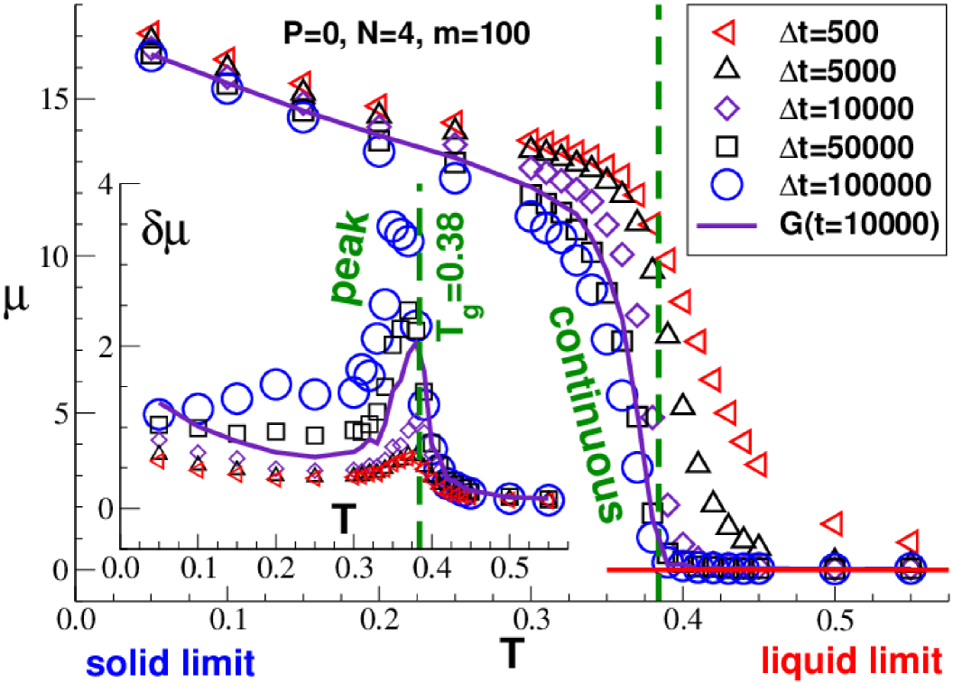
Figure 1: Key findings as a function of temperature $T$. The vertical dashed lines indicate the glass transition temperature $\mbox{$T_{\rm g}$}\approx 0.38$. Main panel: Shear modulus $\mu(T)$ for different sampling times $\Delta t$ showing that the transition becomes more and more step-like with increasing $\Delta t$. Inset: Corresponding standard deviation $\delta\mu(T)$ showing a peak at $T\approx\mbox{$T_{\rm g}$}$ which becomes sharper with increasing $\Delta t$. Also included are the shear stress relaxation modulus $G(t)$ and its standard deviation $\delta G(t)$ taken at a time $t=10^{4}$ (bold solid lines).

Key findings.

Following the pioneering work by Barrat et al. Barrat et al. (1988) and many recent numerical studies Wittmer et al. (2002); Barrat (2006); Schnell et al. (2011); Xu et al. (2012); Wittmer et al. (2013); Li et al. (2016); Procaccia et al. (2016); Kriuchevskyi et al. (2017) we use the stress-fluctuation formalism Squire et al. (1969); Lutsko (1988); Wittmer et al. (2015a, b, c) to determine the shear modulus. Our key findings for $\mu$ and its standard deviation $\delta\mu$, obtained as function of $T$ for a broad range of sampling times $\Delta t$, are summarized in Fig. 1. Albeit $\mu(T)$ remains always continuous, it becomes systematically more step-like with increasing $\Delta t$. At variance to the monotonous modulus $\mu(T)$ its standard deviation $\delta\mu(T)$ is non-monotonous with a remarkable peak near $\mbox{$T_{\rm g}$}\approx 0.38$. (As explained in the SM foo (a), $T_{\rm g}$ is defined here by means of a $\Delta t$-independent dilatometric criterion during the initial continuous temperature quench Schnell et al. (2011); Li et al. (2016).) The peak increases with $\Delta t$, becoming about a third of the drop of $\mu(T)$ between $T=0.34$ and $T=0.38$ for $\Delta t=10^{5}$. The liquid-solid transition is thus accompanied by strong fluctuations between different glass configurations. We corroborate these results below. Especially, we shall trace back the observed $\Delta t$-dependence of $\mu$ to the time dependence of the shear-stress relaxation modulus $G(t)$ Rubinstein and Colby (2003).

Time series.

Our $m=100$ independently quenched configurations contain $3072$ chains of length $N=4$. A vanishing normal pressure ($P=0)$ is imposed for all $T$. Having reached a specific temperature and after tempering over $\Delta t_{\mathrm{max}}=10^{5}$ we perform production runs over again $\Delta t_{\mathrm{max}}$ with entries made each velocity-Verlet sweep. Of importance are here the instantaneous shear stress $\hat{\tau}$ and the instantaneous “affine shear modulus” $\hat{\mu}_{\mathrm{A}}$. As reminded in Sec. 2 of the SM foo (a), $\hat{\tau}$ is the first functional derivative of the Hamiltonian with respect to an imposed infinitesimal canonical and affine shear transformation and $\hat{\mu}_{\mathrm{A}}$ the corresponding second functional derivative Wittmer et al. (2013); Wittmer et al. (2015a, b, c, 2016b, 2016a). The stored time-series are used to compute for a given configuration and shear plane various time-averages Allen and Tildesley (1994) (marked by horizontal bars) over sampling times $\Delta t\leq\Delta t_{\mathrm{max}}$

$$\overline{\mu}_{\mathrm{A}} \equiv \overline{\hat{\mu}_{\mathrm{A}}}$$ (1)

$$\overline{\mu}_{\mathrm{F}} \equiv \overline{\mu}_{0}-\overline{\mu}_{1}\mbox{ with }\overline{\mu}_{0}\equiv\beta V\overline{\hat{\tau}^{2}},\ \overline{\mu}_{1}\equiv\beta V\overline{\hat{\tau}}^{2}$$ (2)

$$\overline{\mu} \equiv \overline{\mu}_{\mathrm{A}}-\overline{\mu}_{\mathrm{F}}\equiv(\overline{\mu}_{\mathrm{A}}-\overline{\mu}_{0})+\overline{\mu}_{1}$$ (3)

with $\beta=1/T$ being the inverse temperature and $V$ the volume of each configuration.

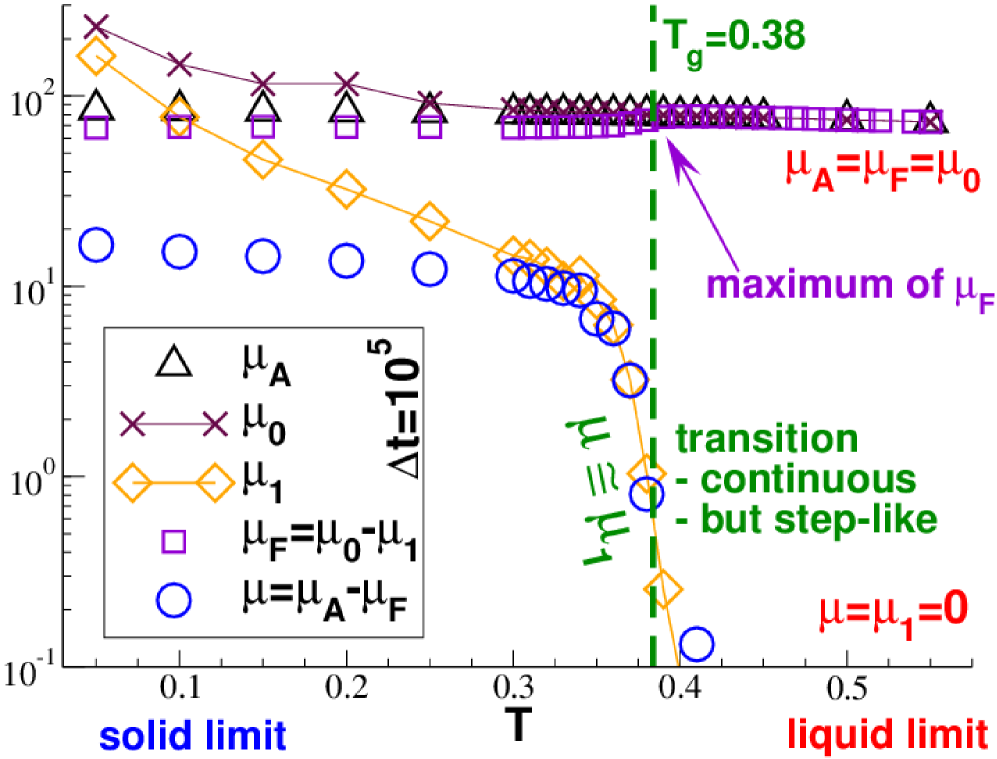
Figure 2: First moments $\mu_{\mathrm{A}}$, $\mu_{0}$, $\mu_{1}$, $\mu_{\mathrm{F}}$ and $\mu$ vs. temperature $T$ using a half-logarithmic representation. The data are obtained for $\Delta t=\Delta t_{\mathrm{max}}=10^{5}$. With decreasing temperature $\mu\approx\mu_{1}$ increases rapidly at $T_{\rm g}$, but remains continuous. Interestingly, $\mu_{0}$ deviates from $\mu_{\mathrm{A}}$ and $\mu_{1}$ from $\mu$ below $T_{\rm g}$.

Expectation values.

The corresponding ensemble averages $\mu_{\mathrm{A}}\equiv\langle\overline{\mu}_{\mathrm{A}}\rangle$, $\mu_{0}\equiv\langle\overline{\mu}_{0}\rangle$, $\mu_{1}\equiv\langle\overline{\mu}_{1}\rangle$, $\mu_{\mathrm{F}}\equiv\langle\overline{\mu}_{\mathrm{F}}\rangle$ and $\mu\equiv\langle\overline{\mu}\rangle$ are then obtained by averaging over the $m$ configurations and the three shear planes foo (b). We have already presented the modulus $\mu(T)$ in the main panel of Fig. 1 using a linear representation. Figure 2 presents $\mu(T)$ and its various contributions for $\Delta t=\Delta t_{\mathrm{max}}=10^{5}$ using half-logarithmic coordinates. As emphasized above, albeit $\mu=\mu_{\mathrm{A}}-\mu_{\mathrm{F}}$ increases rapidly below $T_{\rm g}$, the data remain continuous in line with findings reported for colloidal glass-formers Barrat et al. (1988); Wittmer et al. (2013); Li et al. (2016) using also the stress-fluctuation formula. As one expects $\mu=\mu_{1}=0$ in the liquid limit above $T_{\rm g}$ and, hence, $\mu_{\mathrm{F}}=\mu_{0}=\mu_{\mathrm{A}}$ Wittmer et al. (2013); Wittmer et al. (2015a); Kriuchevskyi et al. (2017). At variance to this, $\mu_{\mathrm{F}}<\mu_{\mathrm{A}}$ below $T_{\rm g}$, i.e. the shear-stress fluctuations do not have sufficient time to fully explore the phase space. In agreement with Lutsko Lutsko (1988) and more recent studies Wittmer et al. (2002); Barrat (2006); Wittmer et al. (2013); Li et al. (2016), $\mu_{\mathrm{F}}$ does not vanish for $T\to 0$, i.e. $\mu_{\mathrm{A}}$ is only an upper bound of $\mu=\mu_{\mathrm{A}}-\mu_{\mathrm{F}}$. We emphasize that while $\mu_{\mathrm{F}}=\mu_{0}-\mu_{1}$ is more or less constant below $T_{\rm g}$, its contributions $\mu_{0}$ and $\mu_{1}$ increase rapidly with decreasing $T$.

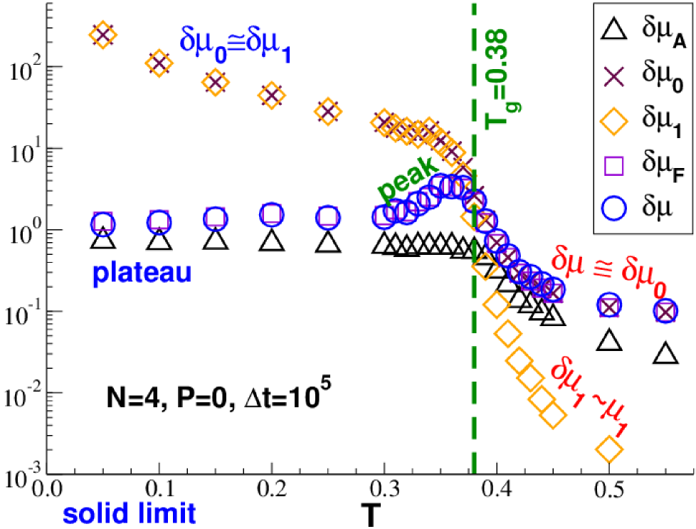
Figure 3: Standard deviations $\delta\mu_{\mathrm{A}}$, $\delta\mu_{0}$, $\delta\mu_{1}$, $\delta\mu_{\mathrm{F}}$ and $\delta\mu$ as a function of $T$. $\delta\mu_{\mathrm{A}}$ is found to be small and $\delta\mu\approx\delta\mu_{\mathrm{F}}$ for all $T$. Below $T_{\rm g}$ the standard deviations $\delta\mu_{1}$ and $\delta\mu_{0}$ become rapidly similar and orders of magnitude larger than $\delta\mu_{\mathrm{F}}$. This confirms the presence of strong frozen shear stresses.

Ensemble fluctuations.

To characterize also the fluctuations between different configurations we take for various properties in addition the second moment over the ensemble. As already seen in the inset of Fig. 1, we thus compute, e.g., the standard deviation of the shear modulus $\delta\mu=\sqrt{\langle\overline{\mu}^{2}\rangle-\langle\overline{\mu}\rangle^{2}}$ foo (b). $\delta\mu$ is presented together with the corresponding standard deviations $\delta\mu_{\mathrm{A}}$, $\delta\mu_{0}$, $\delta\mu_{1}$ and $\delta\mu_{\mathrm{F}}$ in Fig. 3. As can be seen, $\delta\mu_{\mathrm{A}}$ is negligible and $\delta\mu\approx\delta\mu_{\mathrm{F}}$ for all $T$. In the high-$T$ regime we find $\delta\mu\approx\delta\mu_{0}$ while $\delta\mu_{1}\approx\mu_{1}$ vanishes much more rapidly. In the opposite glass-limit $\delta\mu\approx\delta\mu_{\mathrm{F}}$ becomes orders of magnitude smaller than $\delta\mu_{0}\approx\delta\mu_{1}$ Kriuchevskyi et al. (2017). The contributions $\overline{\mu}_{0}$ and $\overline{\mu}_{1}$ of the difference $\overline{\mu}_{\mathrm{F}}=\overline{\mu}_{0}-\overline{\mu}_{1}$ thus must be strongly correlated as one verifies using the corresponding correlation coefficient. This is yet another manifestation of the strong frozen shear stresses which are generated in each configuration while quenching the systems through the glass transition.

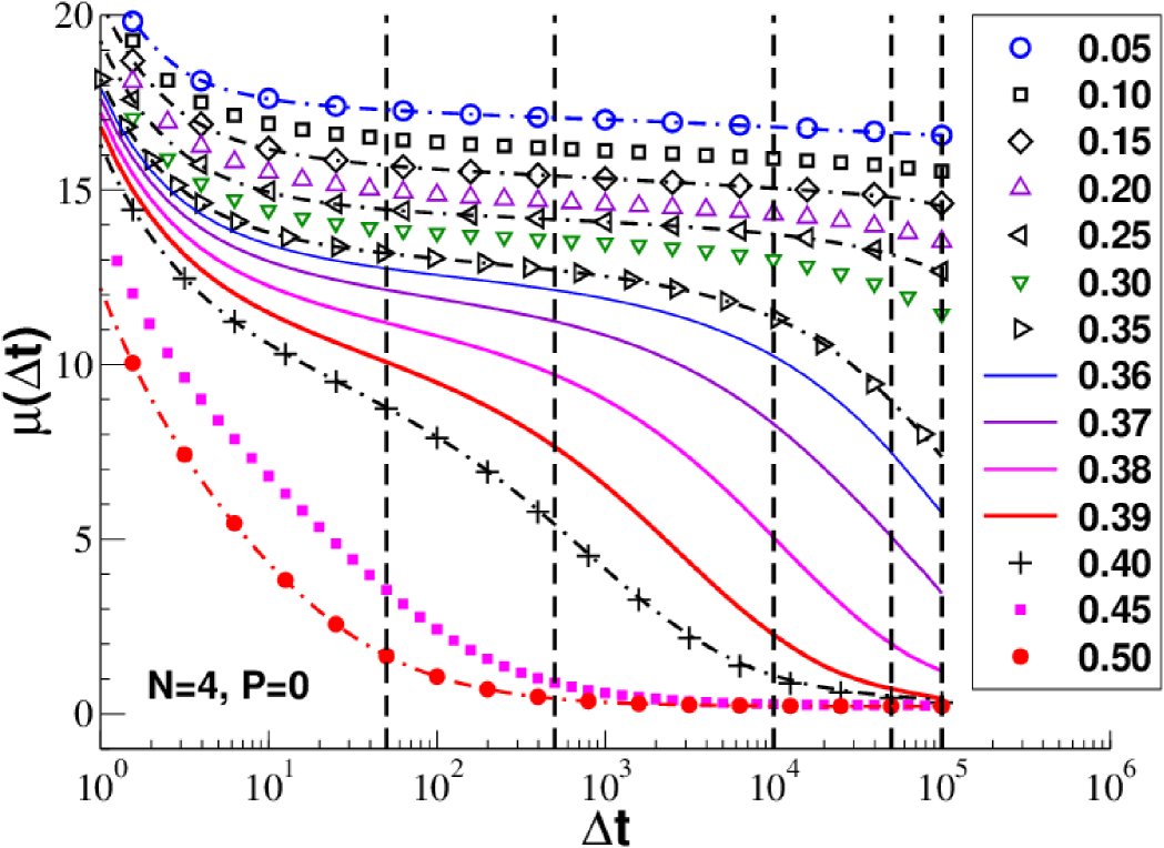
Figure 4: Shear modulus $\mu$ as a function of sampling time $\Delta t$ for a broad range of $T$ as indicated in the figure. $\mu(\Delta t)$ decreases continuously with $\Delta t$. Note that a smaller temperature increment $\Delta T=0.01$ is used around $T_{\rm g}$ (solid lines) where $\mu(\Delta t;T)$ changes much more rapidly with $T$. The dash-dotted lines are obtained using Eq. (4) by integrating the directly measured shear-stress relaxation modulus $G(t)$. The vertical lines mark the sampling times used in Fig. 1.

$\Delta t$-dependence.

We return now to the sampling time dependence shown in Fig. 1. As expected from crystalline and amorphous solids Li et al. (2016); Wittmer et al. (2013) and permanent Wittmer et al. (2013); Wittmer et al. (2016b) and transient Wittmer et al. (2016a) elastic networks, the expectation values of the contributions $\mu_{\mathrm{A}}$ and $\mu_{0}$ to $\mu$ are strictly $\Delta t$-independent (not shown). This can be traced back to the fact that their time and ensemble averages commute Wittmer et al. (2016b); foo (c). This is strikingly different for $\mu_{1}$, $\mu_{\mathrm{F}}$ and $\mu$ for which this commutation relation does not hold. As shown in Fig. 4, we focus here on the $\Delta t$-dependence of $\mu(\Delta t)=(\mu_{\mathrm{A}}-\mu_{0})+\mu_{1}(\Delta t)$. Covering a broad range of temperatures we use subsets of length $\Delta t$ of the total trajectories of length $\Delta t_{\mathrm{max}}$ stored. It is seen that $\mu(\Delta t)$ decreases both monotonously and continuously with $\Delta t$. The figure reveals that $\mu(\Delta t;T)$ decreases also monotonously and continuously with $T$. A glance at Fig. 4 shows that one expects the transition of $\mu(T)$ to get shifted to lower $T$ and to become more step-like with increasing $\Delta t$ in agreement with Fig. 1. (Note that $\mu(\Delta t)$ increases for $T\to 0$ while its decay slows down.) It is, however, impossible to reconcile the data with a jump-singularity at a finite $\Delta t$ and $T$. It is neither possible to achieve a reasonable data collapse by shifting the data.

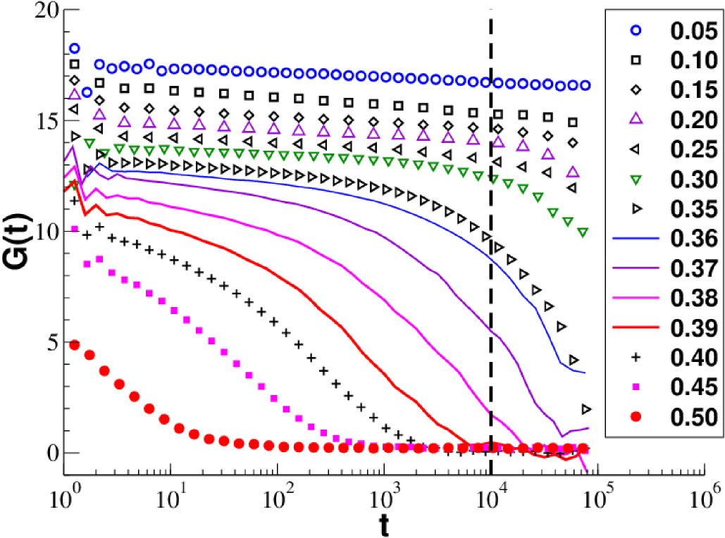
Figure 5: Stress relaxation modulus $G(t)$ for a broad range of $T$. The data are rather similar to the shear modulus $\mu(\Delta t)$ presented in Fig. 4. The dashed vertical line marks the time $t=10^{4}$ used for $G(t)$ and $\delta G(t)$ in Fig. 1.

Connection between $\mu(\Delta t)$ and $G(t)$.

The systematic sampling time dependence of $\mu(\Delta t)$ shown in Fig. 1 and Fig. 4 can be understood from the generic sampling time dependence of time-averaged fluctuations Landau and Binder (2000). Assuming time-translational invariance $\mu(\Delta t)$ may be written as a weighted average Wittmer et al. (2015a, b, c, 2016b, 2016a); Kriuchevskyi et al. (2017)

$$\mu(\Delta t)=\frac{2}{\Delta t^{2}}\int_{0}^{\Delta t}(\Delta t-t)\ G(t)\ \mathrm{d}t,$$ (4)

over the shear-relaxation modulus $G(t)$ foo (a). As shown in Fig. 5, we have computed $G(t)$ directly by means of the fluctuation-dissipation relation appropriate for canonical ensembles with quenched or sluggish shear stresses Wittmer et al. (2015a, 2016b); Kriuchevskyi et al. (2017); foo (a). Having thus characterized the relaxation modulus $G(t)$, the numerical sum corresponding to Eq. (4) yields the thin dash-dotted lines indicated in Fig. 4. Being identical with the stress-fluctuation formula $\mu=\mu_{\mathrm{A}}-\mu_{\mathrm{F}}$ for all $T$, this confirms the assumed time-translational invariance. The $\Delta t$-dependence of $\mu$, $\mu_{1}$ and $\mu_{\mathrm{F}}$ is thus simply due to the upper boundary $\Delta t$ used to average $G(t)$. As one expects from Eq. (4) foo (a), the functional forms of $\mu(\Delta t)$ and $G(t)$ are rather similar, especially at low $T$. Fixing a time $t$, say $t=10^{4}$ as indicated by the vertical dashed line in Fig. 5, allows to characterize the temperature dependence of the relaxation modulus $G(t)$ and its standard deviations $\delta G(t)$ (bold solid lines in Fig. 1). Consistently with Eq. (4), a similar behavior is found as for $\mu(T)$ and $\delta\mu(T)$.

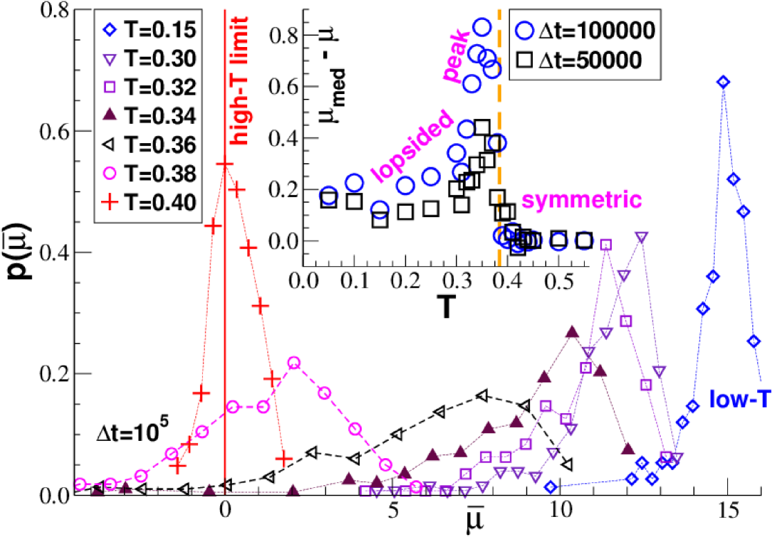
Figure 6: Main panel: Distribution $p(\overline{\mu})$ for $\Delta t=10^{5}$ for different $T$. Inset: Difference $\mu_{\mathrm{med}}-\mu$ of the median $\mu_{\mathrm{med}}$ and the ensemble average $\mu$ vs. $T$ for two sampling times. The difference has a peak slightly below $T_{\rm g}$ corresponding to very lopsided distributions.

Distribution of $\overline{\mu}$.

The striking peak of $\delta\mu$ below $T_{\rm g}$ seen in Fig. 1 begs for a more detailed characterization of the distribution $p(\overline{\mu};T,\Delta t)$ of the time-averaged shear modulus $\overline{\mu}$. Focusing on our largest sampling time $\Delta t_{\mathrm{max}}$, the main panel of Fig. 6 presents normalized histograms obtained using $3\times m=300$ measurements. We emphasize that the histograms are unimodal for all $T$ and $\Delta t$ foo (d). The $T$-dependence of $\mu$ and $\delta\mu$ below $T_{\rm g}$ seen in Fig. 1 is thus not due to, e.g., the superposition of two configuration populations representing either solid states with finite $\overline{\mu}$ and liquid states with $\overline{\mu}\approx 0$. The maximum $\mu_{\mathrm{max}}$ of the (unimodal) distribution systematically shifts to higher values below $T_{\rm g}$, in agreement with its first moment $\mu$ (Fig. 1), while the distributions become systematically broader and more lopsided, i.e. liquid-like configurations with small $\overline{\mu}$ remain relevant. The increase of $\delta\mu$ with sampling time $\Delta t$ seen in the inset of Fig. 1 is due to the broadening of $p(\overline{\mu})$ caused by the growing weight of small-$\overline{\mu}$ configurations (not shown). For even smaller temperatures $T\ll\mbox{$T_{\rm g}$}$, the distributions get again more focused around their maxima $\mu_{\mathrm{max}}$ (as expected from Fig. 1) and less lopsided. That the large standard deviations and the asymmetry of the distributions are related is demonstrated by comparing the first moment $\mu$ of the distribution, its median $\mu_{\mathrm{med}}$ and its maximum $\mu_{\mathrm{max}}$. One confirms that $0<\mu_{\mathrm{med}}-\mu<\mu_{\mathrm{max}}-\mu$ below $T_{\rm g}$ for all $\Delta t$. As seen from the inset of Fig. 6, $\mu_{\mathrm{med}}-\mu$ has a peak similar to $\delta\mu$ becoming sharper with increasing $\Delta t$.

Summary.

We investigated by means of MD simulations a coarse-grained model for polymer glasses characterizing its shear modulus $\mu$ using the stress-fluctuation formalism. The observed $\Delta t$-dependence of $\mu$ (Fig. 1) and its contributions $\mu_{1}$ and $\mu_{\mathrm{F}}$ can be traced back to the finite time (time-averaged) stress fluctuations need to explore the phase space which is perfectly described (Fig. 4) by the weighted integral over the shear-stress relaxation modulus $G(t)$ [Eq. (4)]. The liquid-solid transition characterized by the ensemble-averaged $\mu(T)$ is continuous for all sampling times $\Delta t$, but becomes sharper and thus better defined with increasing $\Delta t$ (Fig. 1). However, while the transition gets more step-like on average, increasingly strong fluctuations between different configurations underly the transition. The broad and lopsided distribution $p(\overline{\mu})$ below $T_{\rm g}$ makes the prediction of the modulus $\overline{\mu}$ of a single configuration elusive (Fig. 6).

Beyond the current study.

While $\mu$ and its contributions $\mu_{\mathrm{A}}$, $\mu_{\mathrm{F}}$, $\mu_{0}$ and $\mu_{1}$ do not depend on the system size foo (a), this is more intricate for the corresponding standard deviations and must be addressed in the future following Ref. Procaccia et al. (2016). Recent work on self-assembled networks Wittmer et al. (2016a) suggests that $\delta\mu\approx\delta\mu_{\mathrm{F}}\sim 1/\sqrt{V}$ for $T\ll\mbox{$T_{\rm g}$}$ (self-averaging), while $\delta\mu\approx\delta\mu_{\mathrm{F}}\sim V^{0}$ around $T_{\rm g}$ (lack of self-averaging). In the latter limit long-ranged elastically interacting activated events are expected to dominate the plastic reorganizations of the particle contacts Ferrero et al. (2014). From a broader vantage point it is no surprise that the lifting of the permutation invariance of the liquid state below $T_{\rm g}$ Alexander (1998) should lead to strong fluctuations between different configurations. The observation of strong frozen-in shear stresses (Figs. 2 and 3) is thus merely a demonstration of the broken symmetry. Analysis tools need to account for these frozen zero-wavevector stresses and theoretical approaches neglecting them are bound to miss the heart of the problem.