Klein–Gordon equation in curved space-time

Abstract

We solve the relativistic Klein–Gordon equation for a light particle gravitationally bound to a heavy central mass, with the gravitational interaction prescribed by the metric of a spherically symmetric space-time. Metrics are considered for an impenetrable sphere, a soft sphere of uniform density, and a soft sphere with a linear transition from constant to zero density; in each case the radius of the central mass is chosen to be sufficient to avoid any event horizon. The solutions are obtained numerically and compared with nonrelativistic Coulomb-type solutions, both directly and in perturbation theory, to study the general-relativistic corrections to the quantum solutions for a $1/r$ potential. The density profile with a linear transition is chosen to avoid singularities in the wave equation that can be caused by a discontinuous derivative of the density.

I Introduction

Although gravity is too weak for there to be, in practice, a gravitational analog of the hydrogen atom,PhaseShift the quantum mechanics of a particle bound gravitationally to a central mass can still be considered theoretically. Of course, the nonrelativistic form of this problem is trivially solved, given that the hydrogen-atom Coulomb solutions are so well known. What is of some interest, however, is how such a problem can be solved in the context of the general theory of relativity, where the gravitational interaction is defined by a space-time metric. The formulation of the problem must then start from a covariant relativistic wave equation, such as the Klein–Gordon (KG) equation or the Dirac equation. For simplicity, we consider the former.

The solution of the KG equation in a curved space-time requires numerical techniques. Earlier work that sought exact solutionsexactKG was inconclusive at best, involving either approximate expansions or simplifying assumptions to obtain asymptotic solutions. On the other hand, numerical methods, such as matrix methods for finite-difference approximations and Runge-Kutta integration combined with boundary-condition matching, are easy to implement to almost any desired accuracy.

Our models are based on static, spherically symmetric metrics of the form

$$ds^{2}=g_{00}(r)dt^{2}-g_{rr}(r)dr^{2}-r^{2}d\theta^{2}-r^{2}\sin^{2}\theta d\phi^{2}.$$ (1)

The classic example is the Schwarzschild metric, for which,units outside the central mass $M$,

$$g_{00}=1-\frac{2GM}{r},\;\;g_{rr}=\left(1-\frac{2GM}{r}\right)^{-1}.$$ (2)

For the impenetrable sphere, the KG wave function is set to zero at the outer radius $r_{0}$ of the mass, with $r_{0}$ always chosen larger than the Schwarzschild radius $r_{S}\equiv 2GM$. For all spherically symmetric models, the Schwarzschild metric is the exterior solution. For the interior of the soft sphere, we use the solutionsoftsphere for a uniform mass density of radius $r_{0}$

$$g_{00}=\frac{1}{4}\left[3\sqrt{f(r_{0})}-\sqrt{f(r)}\right]^{2},\;\;g_{rr}=1/f(r),$$ (3)

with

$$f(r)=1-\frac{r_{S}}{r_{0}^{3}}r^{2}.$$ (4)

For consistency of the model, the radius $r_{0}$ must be greater than $\frac{9}{8}r_{S}$; this is known as the Buchdahl limit.limit As a tensor, the metric is then specified by the diagonal matrices

$$g^{\mu\nu}=\left(\begin{array}[]{cccc}g_{00}&0&0&0\\ 0&-g_{rr}&0&0\\ 0&0&-r^{2}&0\\ 0&0&0&-r^{2}\sin^{2}\theta\end{array}\right),\;\;\;\;g_{\mu\nu}=\left(\begin{array}[]{cccc}1/g_{00}&0&0&0\\ 0&-1/g_{rr}&0&0\\ 0&0&-1/r^{2}&0\\ 0&0&0&-1/r^{2}\sin^{2}\theta\end{array}\right).$$ (5)

Given such a metric, the covariant KG equation $(\nabla^{\mu}g_{\mu\nu}\nabla^{\nu}+m^{2})\Psi=0$ for a mass $m$ takes the form

$$\left[\frac{1}{g_{00}}\frac{\partial^{2}}{\partial t^{2}}-\frac{1}{r^{2}}\frac{\partial}{\partial r}\left(\frac{r^{2}}{g_{rr}}\frac{\partial}{\partial r}\right)+\frac{L^{2}}{r^{2}}+m^{2}\right]\Psi=0,$$ (6)

with $L^{2}$ the operator for total angular momentum. Standard separation of variables, as $\Psi=\tau(t)R_{l}(r)Y_{lm}(\theta,\phi)$ with $Y_{lm}$ the usual spherical harmonics, yields

$$-\frac{1}{\tau}\frac{d^{2}\tau}{dt^{2}}=g_{00}\left[-\frac{1}{r^{2}R_{l}}\frac{d}{dr}\left(\frac{r^{2}}{g_{rr}}\frac{dR_{l}}{dr}\right)+\frac{l(l+1)}{r^{2}}+m^{2}\right]\equiv E^{2},$$ (7)

where $E^{2}$ is the separation constant, chosen such that $E$ is the total energy and $\Delta E\equiv E-m$, the binding energy. The solution for $\tau$ is, of course, trivial: $\tau=e^{\pm iEt}$, and we do not consider it further. Our interest is in the stationary states, with radial wave functions $R_{l}$, and their energy levels.positive

The wave functions are normalized as integrals over the volume of the curved space. The volume of a sphere of radius $r_{0}$ is given by

$$V=\int^{r<r_{0}}\sqrt{|g|}d^{3}r=4\pi\int_{0}^{r_{0}}\sqrt{g_{rr}}r^{2}dr,$$ (8)

where $|g|=g_{rr}r^{4}\sin^{2}\theta$ is the determinant of the spatial part of the metric. Thus the normalization condition for the radial wave function is

$$1=\int|R_{l}|^{2}\sqrt{g_{rr}}r^{2}dr.$$ (9)

In the following section, we discuss the solution of the radial equation for the two models and separate the relativistic corrections to be compared with perturbation theory. In Sec. III we present results for the energies and wave functions, including comparisons with perturbation theory and comparisons between models. The results show that the sharp boundary between the interior and exterior of the soft sphere induces a kink in the wave function; we therefore consider a modification of the model to taper the edge in Sec. IV. A summary of the work and possible extensions are discussed in Sec. V. Details of one derivation are left to an appendix.

II Analysis

As a first step in analyzing the radial KG equation (7), we introduce a modified radial wave function $u_{l}$ such that no first-order derivatives appear. As shown in the Appendix, this is accomplished with the definition $R_{l}=\sqrt{g_{rr}}u_{l}/r$. The radial equation then reduces to

$$-\frac{d^{2}u_{l}}{dr^{2}}-\left[\frac{g^{\prime}_{rr}}{rg_{rr}}+\frac{1}{2}\frac{g^{\prime\prime}_{rr}}{g_{rr}}-\frac{3}{4}\left(\frac{g^{\prime}_{rr}}{g_{rr}}\right)^{2}\right]u_{l}+\frac{l(l+1)}{r^{2}}g_{rr}u_{l}+m^{2}g_{rr}u_{l}=E^{2}\frac{g_{rr}}{g_{00}}u_{l}.$$ (10)

In the exterior region, where the metric is always the Schwarzschild metric, the contents of the square brackets simplifies considerably. The required derivatives are

$$g^{\prime}_{rr}=-\frac{2GM}{r^{2}}\left(1-\frac{2GM}{r}\right)^{-2}=-r_{S}/(r-r_{S})^{2}$$ (11)

and

$$g^{\prime\prime}_{rr}=2r_{S}/(r-r_{S})^{3}.$$ (12)

Substitution of these yields, for $r>r_{0}$,

$$-\frac{d^{2}u_{l}}{dr^{2}}-\frac{1}{4}\frac{r_{S}^{2}}{r^{2}(r-r_{S})^{2}}u_{l}+\frac{l(l+1)}{r^{2}(1-r_{s}/r)}u_{l}+\frac{m^{2}}{1-r_{s}/r}u_{l}=\frac{E^{2}}{(1-r_{s}/r)^{2}}u_{l}.$$ (13)

As discussed more fully below, the leading Coulombic interaction arises not from the second term but from the difference of the $m^{2}$ and $E^{2}$ terms. Here $E$ is the relativistic energy, which includes the rest energy $m$; a nonrelativistic Schrödinger equation would consider the difference, $\Delta E\equiv E-m$. Substitution of the expansion $E^{2}=m^{2}+2m\Delta E+\Delta E^{2}$, combination of the two terms proportional to $m^{2}$, and division by $2m$ leads to

$$-\frac{1}{2m}\frac{d^{2}u_{l}}{dr^{2}}-\frac{1}{4}\frac{r_{S}^{2}}{2mr^{2}(r-r_{S})^{2}}u_{l}+\frac{l(l+1)}{2mr^{2}(1-r_{S}/r)}u_{l}-\frac{mr_{S}}{2r}\frac{1}{(1-r_{S}/r)^{2}}u_{l}=\frac{\Delta E+\Delta E^{2}/2m}{(1-r_{S}/r)^{2}}u_{l}.$$ (14)

The combination $mr_{S}/2$ is just $GMm$. Thus to lowest order in $r_{S}$, the modified radial equation reduces to

$$-\frac{1}{2m}\frac{d^{2}u_{l}}{dr^{2}}+\frac{l(l+1)}{2mr^{2}}u_{l}-\frac{GMm}{r}u_{l}=\Delta Eu_{l},$$ (15)

which is just the standard Schrödinger equation with a Newtonian gravitational potential. We discuss leading corrections to this below.

Given that $GMm$ plays the role of $e^{2}$ in the Coulomb term, the natural length scale for this system is the Bohr radius $a=1/GMm^{2}$. Consequently, we rescale the radial coordinate to a dimensionless variable $\zeta=r/a$ and correspondingly rescale the Schwarzschild radius as $\zeta_{S}=r_{S}/a=2(GMm)^{2}$ and the sphere radius as $\zeta_{0}=r_{0}/a$. The natural energy scale is $GMm/2a$, which leads to a dimensionless binding energy $\epsilon\equiv 2a\Delta E/GMm$. In terms of these dimensionless quantities, the modified radial equation becomes

$$-\frac{d^{2}u_{l}}{d\zeta^{2}}-\left[\frac{g^{\prime}_{rr}}{\zeta g_{rr}}+\frac{1}{2}\frac{g^{\prime\prime}_{rr}}{g_{rr}}-\frac{3}{4}\left(\frac{g^{\prime}_{rr}}{g_{rr}}\right)^{2}\right]u_{l}+\frac{l(l+1)}{\zeta^{2}}g_{rr}u_{l}+m^{2}g_{rr}(1-1/g_{00})u_{l}=(\epsilon+\frac{1}{8}\zeta_{S}\epsilon^{2})\frac{g_{rr}}{g_{00}}u_{l},$$ (16)

with primes now defined to mean differentiation with respect to $\zeta$. It is this equation that we solve numerically.

For ordinary gravity, the effects are extremely small. For an electron bound to a proton, the gravitational fine structure constant $GMm$ is just $3.2\times 10^{-42}$, and the dimensionless Schwarzschild radius is $2\times 10^{-83}$. These small numbers mean that any numerical solution will not be able to resolve any relativistic effects. Only the Coulombic binding energies $\epsilon=-1/n^{2}$ would be calculable. To have meaningful calculations we must assume a much stronger gravitational coupling and consider values of $\zeta_{S}$ no more than a few orders of magnitude less than unity.

We used two methods to solve the modified radial equation, in order to have some basis for checking the work. One method was to integrate the equation both outward and inward to a point near one Bohr radius, at which the log derivative of the wave function was required to match between the two integrations; the values of epsilon for which a match was achieved were the eigenvalues. The integrations were done with an adaptive Runge–Kutta–Fehlberg algorithmDeVries for a system of first order equations equivalent to the given second order equation.

The other method of solution was to apply a simple finite-difference approximation to the equation and thereby convert it to a matrix equation where the eigenvalues of the matrix correspond to $\lambda\equiv\epsilon+\frac{1}{8}\zeta_{S}\epsilon^{2}$ and the eigenvectors determine the wave function at the discrete points used for the finite differences. The actual $\epsilon$ values are obtained by solving the quadratic equation implied by the definition of $\lambda$, which leaves

$$\epsilon=\frac{-1\pm\sqrt{1+\zeta_{S}\lambda/2}}{\zeta_{S}/4}.$$ (17)

To be consistent with the limit that $\epsilon$ equal $\lambda$ when $\zeta_{S}$ goes to zero, the upper sign is chosen, and to facilitate this limit computationally, we rearrange the expression as

$$\epsilon=\frac{2\lambda}{1+\sqrt{1+\zeta_{S}\lambda/2}}$$ (18)

to avoid the indeterminant $0/0$. The accuracy of the eigenvalues is improved by Richardson extrapolationDeVries from a set of different grid spacings.

As another check on the calculations, we consider first-order perturbation theory for the leading relativistic contributions for the case of the impenetrable sphere. From (14) or (16), the dimensionless form of the radial equation can be seen to be

$$-\frac{d^{2}u_{l}}{d\zeta^{2}}-\frac{1}{4}\frac{\zeta_{S}^{2}}{\zeta^{2}(\zeta-\zeta_{S})^{2}}u_{l}+\frac{l(l+1)}{\zeta^{2}(1-\zeta_{S}/\zeta)}u_{l}-\frac{2}{\zeta}\frac{1}{(1-\zeta_{S}/\zeta)^{2}}u_{l}=\frac{\epsilon+\frac{1}{8}\zeta_{S}\epsilon^{2}}{(1-\zeta_{S}/\zeta)^{2}}u_{l}.$$ (19)

Keeping $\zeta_{S}$ to first order, we obtain

$$-\frac{d^{2}u_{l}}{d\zeta^{2}}+\frac{l(l+1)}{\zeta^{2}}(1+\zeta_{S}/\zeta)u_{l}-\frac{2}{\zeta}(1+2\zeta_{S}/\zeta)u_{l}=(\epsilon(1+2\zeta_{S}/\zeta)+\frac{1}{8}\zeta_{S}\epsilon^{2})u_{l}.$$ (20)

If we collect all of the ${\cal O}(\zeta_{S})$ corrections into a perturbing potential, with $\epsilon$ replaced by its leading value $-1/n^{2}$,

$$V_{S}(\zeta)=\zeta_{S}\left[\frac{l(l+1)}{\zeta^{3}}-\frac{4}{\zeta^{2}}+\frac{1}{n^{2}}\frac{2}{\zeta}-\frac{1}{8}\frac{1}{n^{4}}\right],$$ (21)

the radial equation with this first order correction reads

$$-\frac{d^{2}u_{l}}{d\zeta^{2}}+\frac{l(l+1)}{\zeta^{2}}u_{l}-\frac{2}{\zeta}u_{l}+V_{S}u_{l}=\epsilon u_{l}.$$ (22)

If we keep the central radius $r_{0}$ small and ignore the small deviation from a pure Coulomb interaction inside $r_{0}$, where the zero-order potential is infinite, the zero-order part of this equation yields $-1/n^{2}$ as the zero-order eigenvalue, and the shift due to $V_{S}$ is $\langle u_{l}|V_{S}|u_{l}\rangle$, with $u_{l}$ approximated by the standard hydrogenic modified radial wave functions. For these wave functions, the expectation values of powers of $\zeta$ are known. We need

$$\langle\frac{1}{\zeta}\rangle=\frac{1}{n^{2}},\;\;\langle\frac{1}{\zeta^{2}}\rangle=\frac{1}{(l+1/2)n^{3}},\;\;\langle\frac{1}{\zeta^{3}}\rangle=\frac{1}{(l(l+1)(l+1/2)n^{3}}.$$ (23)

On substitution, they provide

$$\langle V_{S}\rangle=\frac{\zeta_{S}}{(l+1/2)n^{4}}\left[\frac{15}{8}(l+1/2)-3n\right].$$ (24)

This can be compared to shifts in the numerical eigenvalues of the full radial equation as $\zeta_{S}$ is varied. The approximations made are very good for nonzero angular momentum states, for which the wave function does not significantly explore the small-$r$ region, due to the repulsive $1/r^{2}$ term.

III Results

The comparison with perturbation theory is shown in Table 1, where the coefficient of $\zeta_{S}$ in $\langle V_{S}\rangle$ is extracted as the slope of a least-squares fit to a line. Here we see that the predictions for $l=1$ and $l=2$ are quite close. For $l=0$ the agreement is not very good, but this is due to the corrections that should be made for small radii, where the Coulombic solution, used to compute the energy shift, is a poor approximation.

Table 1: Comparison with perturbation theory for the lowest energy levels, $\epsilon_{l+1}$, for the impenetrable sphere. The slopes relative to $\zeta_{S}$, and the associated errors, were computed by a least-squares fit. The theory estimate is given by Eq. (24) of the text.

$\zeta_{S}$	$\zeta_{0}$	$l=0$	$l=1$	$l=2$
0	0	-1	-0.25	-0.11111
0.005	0.0051	-1.0122	-0.25067	-0.11122
0.010	0.011	-1.0223	-0.25134	-0.11132
0.015	0.016	-1.0383	-0.25203	-0.11143
0.020	0.021	-1.0558	-0.25272	-0.11154
0.030	0.031	-1.0951	-0.25414	-0.11176
slope		-3.37$\pm$0.21	-0.1389$\pm$0.0009	-0.0217$\pm$0.0002
theory estimate		-4.125	-0.1328	-0.0213

Tables 2 and 3 list some binding energies computed for each model for similar values of the parameters, $\zeta_{0}$ and $\zeta_{S}$. The radius of the sphere $\zeta_{0}$ is held fixed at 0.5, which corresponds to 1/2 of a Bohr radius. The Schwarzschild radius $\zeta_{S}$, which parameterizes the strength of the relativistic effects, is varied. The effect on the ground state is quite striking, particularly for the soft sphere. In contrast, the lowest $l=2$ state remains almost unaffected, with all values very close to the Coulombic $-1/9$. Between the two models, the soft sphere has the more deeply bound states; the repulsive hard sphere acts to push the particle outward and out of the deeper regions of the effective potential.

Table 2: Dimensionless binding energies for an impenetrable sphere of radius $\zeta_{0}=0.5$.

	$l=0$			$l=1$		$l=2$
$\zeta_{S}$	$\epsilon_{1}$	$\epsilon_{2}$	$\epsilon_{3}$	$\epsilon_{2}$	$\epsilon_{3}$	$\epsilon_{3}$
0	-0.4891	-0.1683	-0.0845	-0.2431	-0.1087	-0.1111
0.01	-0.4933	-0.1695	-0.0850	-0.2443	-0.1092	-0.1113
0.10	-0.5369	-0.1813	-0.0896	-0.2565	-0.1139	-0.1133
0.20	-0.6042	-0.1992	-0.0965	-0.2737	-0.1204	-0.1158
0.30	-0.7112	-0.2269	-0.1067	-0.2981	-0.1296	-0.1184
0.40	-0.9339	-0.2836	-0.1265	-0.3427	-0.1463	-0.1214

Table 3: Same as Table 2 but for the soft-sphere model.

	$l=0$			$l=1$		$l=2$
$\zeta_{S}$	$\epsilon_{1}$	$\epsilon_{2}$	$\epsilon_{3}$	$\epsilon_{2}$	$\epsilon_{3}$	$\epsilon_{3}$
0	-0.899	-0.237	-0.107	-0.250	-0.1111	-0.1111
0.01	-0.936	-0.243	-0.109	-0.251	-0.1116	-0.1113
0.10	-1.517	-0.319	-0.132	-0.266	-0.1173	-0.1133
0.20	-2.970	-0.453	-0.167	-0.293	-0.1273	-0.1158
0.30	-5.256	-0.651	-0.218	-0.542	-0.2148	-0.1184
0.38	-7.701	-1.703	-0.543	-3.157	-0.3246	-0.1208
0.40	-8.646	-3.001	-0.769	-4.158	-0.4202	-0.2619

Some of the corresponding wave functions are plotted in Figs. 1-7. Figure 1 compares the wave functions for the two models with the standard Coulomb solution, for a sphere with a small radius and a very small Schwarzschild radius. The most significant difference is between the impenetrable sphere and the other two cases, where the wave function for the impenetrable sphere is pushed outward relative to the other two.

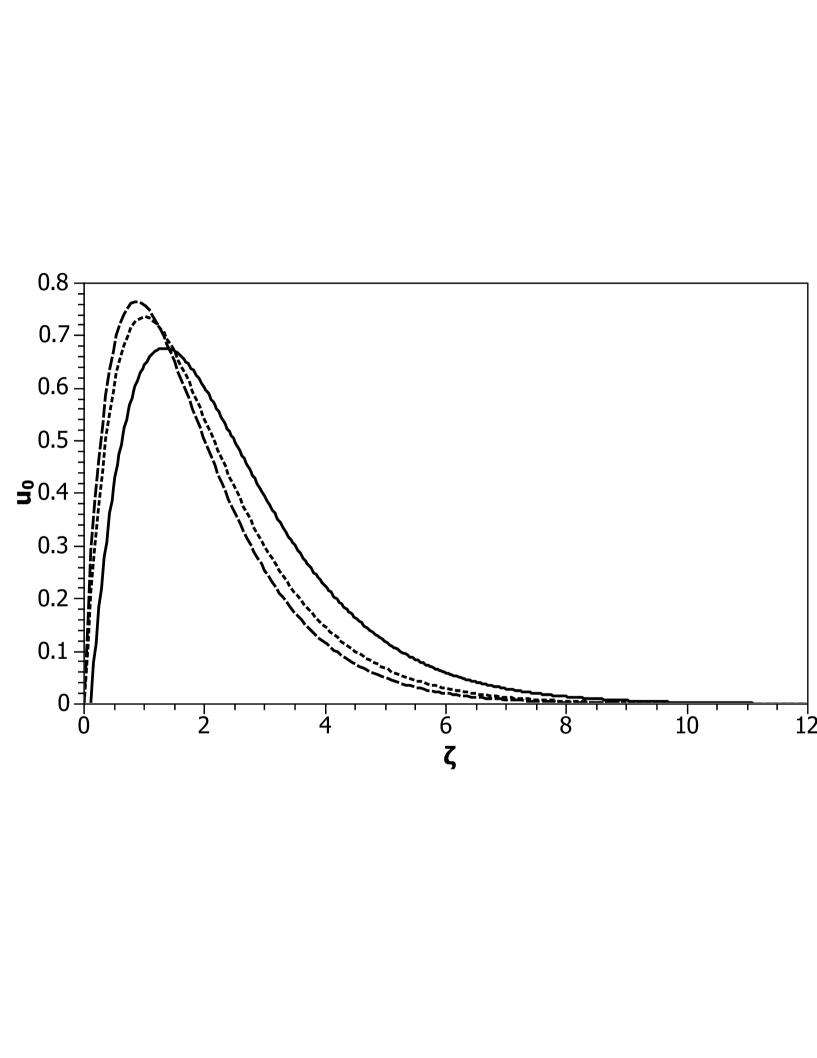
Figure 1: Comparison of wave functions $u_{0}$ for the impenetrable sphere (solid), soft sphere (dashed) and nonrelativistic Coulomb limit (dotted) with $\zeta_{0}=0.1$ as the radius of each sphere and $\zeta_{S}=0.01$ as the Schwarzschild radius, all for zero angular momentum. The radial coordinate $\zeta$ is scaled by the Bohr radius.

Figure 2 shows the evolution of the impenetrable-sphere wave function as the relativistic effects are increased. As the Schwarzschild radius increases, the wave function moves in, closer to the sphere. The same process takes place for the soft-sphere model, as shown in Fig. 3. Here, however, we see that the discontinuity in the derivative of the metric that occurs at the sphere boundary, at $\zeta=\zeta_{0}$, does induce a kink in the wave function; for the highly relativistic cases, with larger $\zeta_{S}$ values, the kink becomes a sharp peak at the sphere radius.

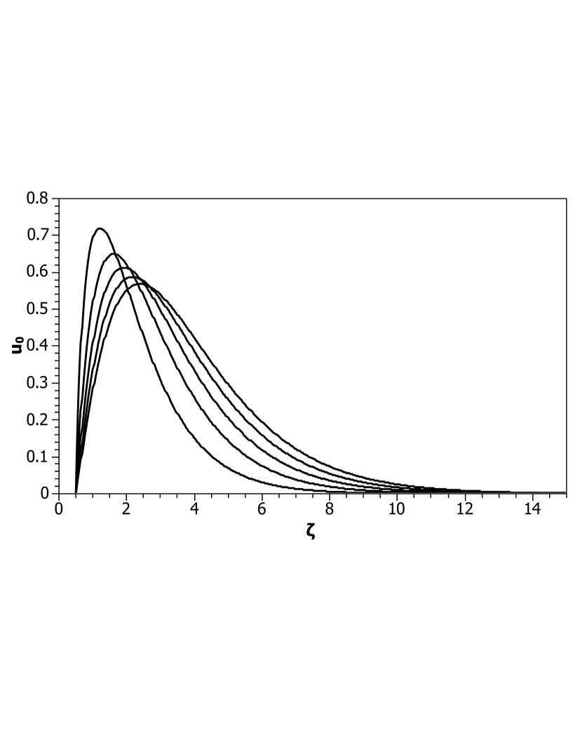
Figure 2: Wave functions $u_{0}$ for an impenetrable sphere of radius $\zeta_{0}=0.5$ with varying Schwarzschild radii $\zeta_{S}=0$, 0.1, 0.2, 0.3, and 0.4 and zero angular momentum. As $\zeta_{S}$ increases, the peak moves to the left.

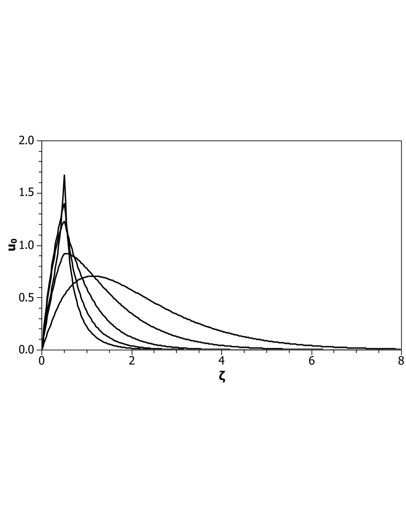
Figure 3: Same as Fig. 2 but for the soft sphere. As $\zeta_{S}$ increases, the peak becomes sharper. The discontinuity in the derivative at the sphere radius is due to discontinuities in the derivatives of the metric.

Comparisons of radially and rotationally excited states can be found in Figs. 4-7. The value of $\zeta_{S}$ is such that the model is highly relativistic. The radially excited states show the standard nodal structure, and the different angular momentum states show the effect of exclusion by the $l(l+1)/r^{2}$ contribution to the effective potential. The kink in the soft-sphere wave functions at the sphere boundary becomes less pronounced for radially excited states, for which the greater probability has moved away from the sphere.

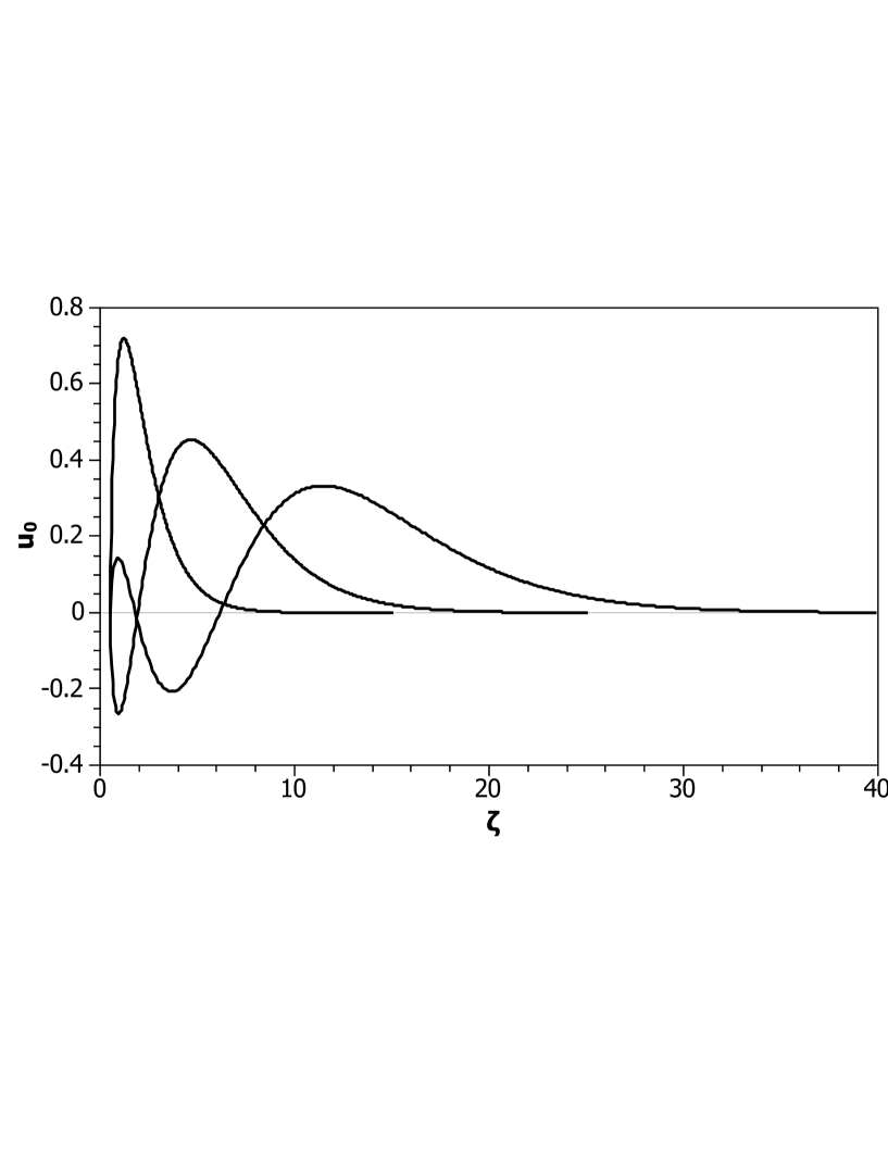
Figure 4: Wave functions $u_{0}$ for three lowest levels of an impenetrable sphere of radius $\zeta_{0}=0.5$ with Schwarzschild radius $\zeta_{S}=0.4$ and zero angular momentum.

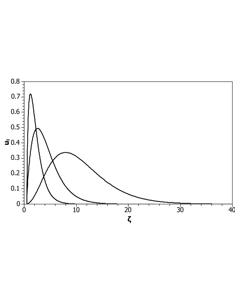
Figure 5: Wave functions $u_{l}$ for the lowest level of an impenetrable sphere of radius $\zeta_{0}=0.5$ with Schwarzschild radius $\zeta_{S}=0.4$ and angular momentum $l=0,1,2$.

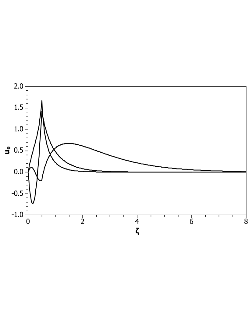
Figure 6: Same as Fig. 4 but for the soft sphere.

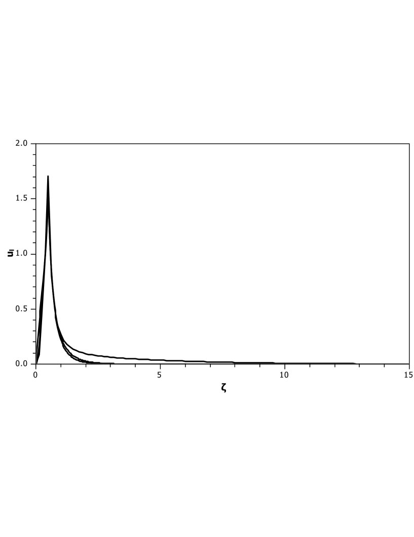
Figure 7: Same as Fig. 5 but for the soft sphere.

IV Continuous density function

To avoid the sharp discontinuity in the density $\rho$, we consider a more realistic behavior that models a gradual transition with the simple form

$$\rho(r)=\left\{\begin{array}[]{ll}\rho_{0},&r\leq r_{0}-\delta\\ (r-r_{0}-\delta)/(2\delta),&r_{0}-\delta<r\leq r_{0}+\delta\\ 0,&r_{0}+\delta<r\end{array}\right.$$ (25)

plotted in Fig. 8.

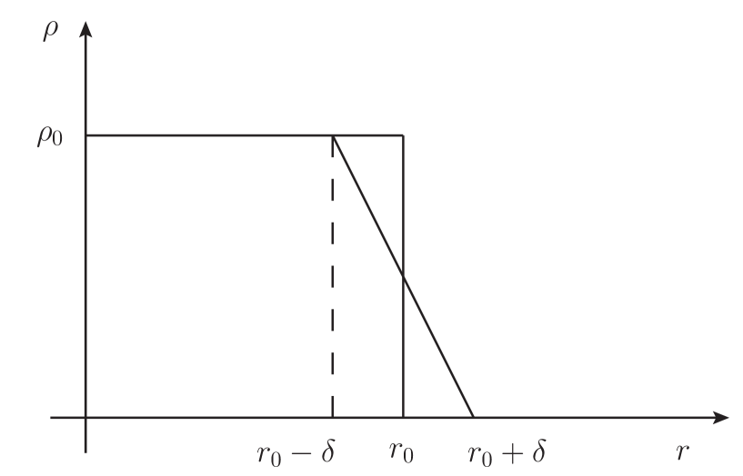
Figure 8: Mass density model with a gradual transition to zero compared to the discontinuous form with a sharp boundary at $r_{0}$.

The parameter $\delta$ controls the width of the transition and $\rho_{0}$, the normalization. The mass inside a spherical surface of area $4\pi r^{2}$ is

$$\mu(r)=\int_{0}^{r}4\pi r^{2}\rho(r)dr,$$ (26)

with the total mass being $M=\mu(\infty)$; this fixes $\rho_{0}$ in proportion to $M$. For the model, the integral is easily done analytically.

Next, we construct the metric corresponding to this density profile. The radial part of the metric is determined asexact

$$g_{rr}=[1-2G\mu(r)/r]^{-1}.$$ (27)

At large $r$, this reduces to the Schwarzschild expression, given in (2). The time component $g_{00}\equiv e^{2\Phi(r)}$ is determined implicitly by the differential equationexact

$$\frac{d\Phi}{dr}=G\frac{\mu(r)+4\pi r^{3}p(r)}{r(r-2G\mu(r))}$$ (28)

and the boundary condition $\Phi(r)\sim\ln\sqrt{1-2G\mu(r)/r}$ for large $r$, again from the Schwarzschild metric (2). Here $p(r)$ is the pressure, which is determined by the Tolman–Oppenheimer–Volkov (TOV) equationexact

$$\frac{dp}{dr}=-G\frac{(\rho(r)+p(r))(\mu(r)+4\pi r^{3}p(r))}{r(r-2G\mu(r))}$$ (29)

and the boundary condition $p(\infty)=0$. This differential equation must be solved first, so that $p(r)$ is available for use in the equation for $\Phi$.

In terms of the dimensionless radial coordinate $\zeta=r/a$ and Schwarzschild radius $\zeta_{S}=2GM/a$, these equations reduce to

$$\tilde{\mu}(\zeta) = 3\int_{0}^{\zeta}\zeta^{2}\tilde{\rho}d\zeta,$$ (30)

$$\frac{d\Phi}{d\zeta} = \frac{\zeta_{S}}{2}\frac{\tilde{\mu}(\zeta)+3\zeta^{3}\tilde{p}(\zeta)}{\zeta[\zeta-\zeta_{S}\tilde{\mu}(\zeta)]},$$ (31)

$$\frac{d\tilde{p}}{d\zeta} = -\frac{\zeta_{S}}{2}\frac{[\tilde{\rho}(\zeta)+\tilde{p}(\zeta)][\tilde{\mu}(\zeta)+3\zeta^{3}\tilde{p}(\zeta)]}{\zeta[\zeta-\zeta_{S}\tilde{\mu}(\zeta)]},$$ (32)

with $\tilde{\mu}\equiv\mu/M$, $\tilde{\rho}\equiv\frac{4\pi a^{3}}{3M}\rho$, and $\tilde{p}\equiv\frac{4\pi a^{3}}{3M}p$. The boundary conditions become

$$\tilde{\mu}(\infty)=1,\;\;\Phi(\zeta)\sim\ln\sqrt{1-\zeta_{S}\tilde{\mu}/\zeta},\;\;\tilde{p}(\infty)=0.$$ (33)

For computational purposes, we model these conditions as occurring at a finite $\zeta_{\rm max}\gg\zeta_{0}$:

$$\tilde{\mu}(\zeta_{\rm max})=1,\;\;\Phi(\zeta_{\rm max})=\ln\sqrt{1-\zeta_{S}/\zeta_{\rm max}},\;\;\tilde{p}(\zeta_{\rm max})=0.$$ (34)

The differential equations are solved by the RK2 Modified Euler method,DeVries in order to have a discretization error consistent with the finite-difference approximation used to solve the radial wave equation (16). The equation for $\tilde{\mu}$ is integrated outward from zero, and the solution renormalized to match the boundary condition. The equations for $\Phi$ and $\tilde{p}$ are integrated inward from $\zeta_{\rm max}$. In the limit that $\delta$ goes to zero, the analytic solution (3) for the metric is obtained, as a check on the calculations.

As input to the radial wave equation, we need derivatives of the metric function $g_{rr}=[1-\zeta_{S}\tilde{\mu}/\zeta]^{-1}$. With use of $d\tilde{\mu}/d\zeta=3\zeta^{2}\rho$, we obtain

$$g^{\prime}_{rr}=\zeta_{S}\frac{3\zeta^{3}\tilde{\rho}-\tilde{\mu}}{(\zeta-\zeta_{S}\tilde{\mu})^{2}}$$ (35)

and

$$g^{\prime\prime}_{rr}=\frac{2\zeta_{S}^{2}(\tilde{\mu}/\zeta^{2}-3\zeta\tilde{\rho})^{2}}{(1-\zeta_{S}\tilde{\mu}/\zeta)^{3}}+\frac{\zeta_{S}(2\tilde{\mu}/\zeta^{3}+3\zeta d\tilde{\rho}/d\zeta)}{(1-\zeta_{S}\tilde{\mu}/\zeta)^{2}}.$$ (36)

For our model, $d\tilde{\rho}/d\zeta$ is computed analytically.

A sampling of the results is given in Table 4 and Fig. 9. The table shows that the gradual transition has a very immediate effect on the ground state eigenenergy. The entry for $\delta=0$ is just the previous result for the sharp boundary. For all nonzero values of $\delta$ the binding energy is significantly less. The wave functions are also greatly altered in the region of the transition. As can be seen in Fig. 9, the kink is eliminated and the peak nicely rounded when $\delta$ is nonzero.

Table 4: Dimensionless binding energies for a sphere of nominal radius $\zeta_{0}=0.5$ with a linear transition from constant density inside $\zeta_{0}-\delta/a$ to zero outside $\zeta_{0}+\delta/a$. Results are given only for $S$ states and for a dimensionless Schwarzschild radius of $\zeta_{S}=0.3$.

$\delta/a$	0	0.005	0.01	0.02	0.05
$\epsilon_{1}$	-5.256	-3.196	-3.192	-3.182	-3.099

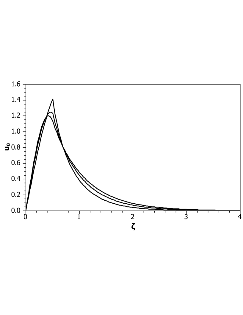
Figure 9: Wave functions $u_{0}$ for the lowest level for a sphere with a gradual transition to zero density, with nominal radius $\zeta_{0}=0.5$, Schwarzschild radius $\zeta_{S}=0.4$, and zero angular momentum. The transition parameter $\delta$ takes three values, $0.05a$, $0.005a$ and 0, the last being the sharp transition with a kink in the wave function. The wave function for the smaller nonzero value has the higher, rounded peak.

V Summary

We have shown that solutions of the KG equation in curved space-time can be computed with ordinary numerical methods and that the results are consistent with the nonrelativistic limit. The results for binding energies are summarized in Tables 2, 3, and 4. The scale of relativistic effects is set by the dimensionless Schwarzschild radius $\zeta_{S}=2GM/a=(2GMm)^{2}$. The binding becomes much stronger as $\zeta_{S}$ is increased, particularly for the soft sphere, where the particle can penetrate the region of nonzero mass density. The addition of a linear transition reduces this effect, primarily because the discontinuity in the metric derivative created an artificially strong binding at the sharp boundary of the soft sphere. The associated wave functions are compared in a series of figures, including Fig. 9 which shows the distinction between soft spheres with and without the linear transition in density.

This work can be extended in at least two ways that would make nice projects for advanced undergraduates and beginning graduate students. One is to consider more sophisticated density profiles. The developments presented here can be immediately carried over, though an accurate calculation may require that the numerical techniques be more sophisticated, depending on the model chosen. The other extension is to consider instead the Dirac equation, in order to treat spin-1/2 particles instead of the spin-0 type represented by the KG equation. This would of course require a new analysis in parallel with the analysis presented here, except that the equations determining the metric from the density profile would remain the same.

*

Appendix A Reduction of the radial equation

In order to eliminate the first-order derivative from the radial equation (7), we write the radial wave function $R_{l}(r)=u_{l}(r)/h(r)$ in terms of a modified radial wave function $u_{l}$ and a function $h(r)$ to be determined. In the ordinary nonrelativistic Coulomb case $h$ is known to be simply equal to $r$, but that would not be sufficient here. The term in (7) that depends on derivatives of $R_{l}$ is

$$\frac{1}{r^{2}}\frac{d}{dr}\left(\frac{r^{2}}{g_{rr}}\frac{dR_{l}}{dr}\right)=\frac{1}{g_{rr}}\frac{d^{2}R_{l}}{dr^{2}}+\left(\frac{2}{g_{rr}}-\frac{g^{\prime}_{rr}}{g_{rr}^{2}}\right)\frac{dR_{l}}{dr}.$$ (37)

Substitution of $R_{l}(r)=u_{l}(r)/h(r)$ yields

$$\frac{1}{r^{2}}\frac{d}{dr}\left(\frac{r^{2}}{g_{rr}}\frac{dR_{l}}{dr}\right)=\frac{1}{hg_{rr}}\left\{\frac{d^{2}u_{l}}{dr^{2}}+\left[\frac{2}{r}-\frac{2h^{\prime}}{h}-\frac{g^{\prime}_{rr}}{g_{rr}}\right]\frac{du_{l}}{dr}-\left[\frac{h^{\prime\prime}}{h}-\frac{2(h^{\prime})^{2}}{h^{2}}+\frac{2h^{\prime}}{rh}-\frac{h^{\prime}g^{\prime}_{rr}}{hg_{rr}}\right]u_{l}\right\}.$$ (38)

The coefficient of $\frac{du_{l}}{dr}$ will be zero if $2hg_{rr}-2rh^{\prime}g_{rr}-rhg^{\prime}_{rr}=0$ or

$$\frac{h^{\prime}}{h}=\frac{1}{r}-\frac{1}{2}\frac{d}{dr}\ln g_{rr}.$$ (39)

This can be directly integrated to obtain the logarithm of the solution, $h=r/\sqrt{g_{rr}}$.

- (1) For a gravitational effect on a wave function that is detectable, see P Asenbaum, C Overstreet, T Kovacky, D D Brown, J M Hogan, and M A Kasevich, “Phase shift in an atom interferometer due to spacetime curvature across its wave function,” Phys. Rev. Lett. 118, 183602 (2017).
- (2) D J Rowan and G Stephenson, “Solutions of the time-dependent Klein-Gordon equation in a Schwarzschild background space,” J. Phys. A: Math. Gen. 9, 1631–1635 (1976); E. Elizalde, “Series solutions for the Klein-Gordon equation in Schwarzschild space-time,” Phys. Rev. D 36, 1269–1272 (1987); “Exact solutions of the massive Klein-Gordon-Schwarzschild equation,” Phys. Rev. D 37, 2127–2131 (1988).
- (3) We use units in which and , but not .
- (4) R.C. Tolman, “Static solutions of Einstein’s field equations for spheres of fluid,” Phys. Rev. 55, 364–373 (1939); M. Blau, “Lecture notes on general relativity,” http://www.blau.itp.unibe.ch/Lecturenotes.html.
- (5) H.A. Buchdahl, “General relativistic fluid spheres,” Phys. Rev. 116, 1027–1034 (1959).
- (6) Only positive energy solutions are considered. The negative energies from the negative square root require field theory for their interpretation in terms of antiparticles.
- (7) P.L. DeVries and J.E. Hasbun, A First Course in Computational Physics, 2e (Jones and Bartlett, 2011).
- (8) J.B. Griffiths and J. Podolsky, Exact Space-Times in Einstein’s General Relativity, (Cambridge University Press, 2009).