On Game-Theoretic Risk Management (Part Three)

Abstract

Abstract

The game-theoretic risk management framework put forth in the precursor reports “Towards a Theory of Games with Payoffs that are Probability-Distributions” (arXiv:1506.07368 [q-fin.EC]) and “Algorithms to Compute Nash-Equilibria in Games with Distributions as Payoffs” (arXiv:1511.08591v1 [q-fin.EC]) is herein concluded by discussing how to integrate the previously developed theory into risk management processes. To this end, we discuss how loss models (primarily but not exclusively non-parametric) can be constructed from data. Furthermore, hints are given on how a meaningful game theoretic model can be set up, and how it can be used in various stages of the ISO 27000 risk management process. Examples related to advanced persistent threats and social engineering are given. We conclude by a discussion on the meaning and practical use of (mixed) Nash equilibria equilibria for risk management.

1 Introduction

With algorithmic matters of game-theoretic risk management being covered in [37], it remains to discuss a few (among more existing) possibilities of how game models can be used in risk management.

First, observe that matrix games directly cover plain optimization as the special case of an either $n\times 1$ or $1\times m$ game. Both have applications in risk management, such as helping with the following common subtasks:

• If the current security configuration is to be assessed against a number $m$ of (new) threats, we can think of the defender having only 1 strategy (the current state). The equilibrium in terms of the $\preceq$-ordering is then the most severe threat (since the attacker maximizes).

• Likewise, if several options for mitigating a particular threat are available, then the equilibrium being the $\preceq$-minimum determined by the defender, is the action leaving the $\preceq$-least damage when being mounted.

• The general case of $n>1$ and $m>1$ strategies for both, the defender and attacker, is discussed in the remainder of this article.

Unique Selling Points:

The method described in the following offers a variety of advantages relative to the “conventional” approach to managing risks, which is usually tied to intensive discussion (meetings), and also up to difficult consensus finding. On the contrary, we propose a method that is based on questioning experts individually, separately, asynchronously and anonymously, which entails the following features, among well known improvement of the so-obtained data quality [31]:

1. Distributed expert interviews that do not require to be at a certain room at a certain time (no meetings), and thus allow provide input in between the normal workflow (asynchronously to the input of other experts).

2. Since the questioning is done individually, it can be done anonymized. This avoids social or cultural effects that may change a person’s statement spoken out loud in presence of certain other people (superiors, subordinates, etc.)

3. Exploitation of matrix organization: it may well be the case that experts are well informed about certain aspects of a problem, but have no reliable clue on some other aspects. Polling people by online questionnaires in the privacy of their own office allows them to answer only those parts of the survey that they can offer input for, while leaving them a safe way of refraining from answering other questions. Since our method works on probability distributions, the resulting dataset from which these are compiled may be richer or sparser, depending on how many informed opinions are available. In any case, however, asking people face-to-face in a meeting can bring up an uninformed guess just to have said something, so that the overall data quality is not necessarily as good as in a distributed and individual interview.

4. Enlargement of the opinion pool: without the need for a personal (and confidential) meeting, people even outside the company can be included in the risk assessment. For example, matters of reputation can more reliably be assessed by customers (which are typically not invited to internal management meetings).

5. The use of distributions also avoids problems of consensus finding or opinion pooling (see, e.g., [20, 5] to mention only two out of many publications in this area) towards a representative number. It is in that sense preserving all information, since all opinions (all available data) goes into the decision process with equal weight.

As a final pro that a game theoretic risk assessment allows, it is even possible to offer the game solution algorithms as a webservice, where the modeling and threat assessment can be left to the customer enterprise. For example, if the client has identified a set of threats and countermeasures, it will prefer to not disclose this information to a subcontractor in charge of risk management. Since the game model and solution can be formulated using abstract names only, it is possible to anonymize the data by letting the threats be only named “T1”, “T2”, …, “Tn”, as well as the countermeasures be called “C1”, “C2”, …, “Cm”. The real meaning of threats and countermeasures can then remain private information of the company, whereas the game model being given in terms of these abstract identifiers remains solvable by any third party contractor. This allows the method to be offered as a (web-)service, without running into troubles of unwanted information disclose (even the number of threats and countermeasures can be disguised, if a company adds dummy copies of actions to the list to make it longer than it actually is).

2 Game-Theory based Risk Management

An eloquent and detailed comparison of how game theory fits into and aids the classical risk management process has been given by [34]. We follow their presentation hereafter, while instantiating and adapting the specific steps to the concrete setting outlined in the precursor parts to this work [35, 37].To get started, consider the classical ISO risk management process as depicted in Figure 1, and compare it to the workflow to be completed when a game-theoretic model is to be set up; shown in Figure 2.

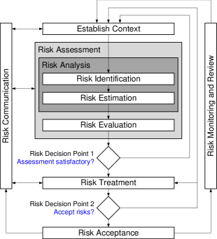
Figure 1: ISO/IEC 27005 Risk Management Process [16]

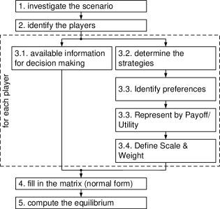
Figure 2: Workflow of setting up a Game Theoretic Model (cf. [34])

The workflow in Figure 2 needs some explanation, in order to establish a mapping to the risk management process. Perhaps the most important difference between risk management and game theory is the former being about minimization of losses caused by a not necessarily rational opponent (nature, but possibly also a hostile party that has explicit intentions). Contrary to this, game theory in any case assumes a rational opponent, whose goal is maximizing the own revenue. A conflict/competition arises if the revenues for both players are negatively correlated, in the extreme case culminating in the well-known zero-sum competition, meaning “my gain is your loss” (and vice versa). This is the scenario that we also assume for risk management based on distribution-valued game theory, although bearing in mind that the incidents that the risk management refers to may not always follow a hidden rationale or agenda. Nevertheless, the zero-sum assumption (even though perhaps unrealistic) provides us with a valid worst-case assessment, and reality can only look better than predicted for the risk manager. The players engaging in the risk management process may be diverse and many, depending on the variety of threats to be considered. In mapping this to a game-theoretic model, we collect all physically existing opponents into a single adversary acting as “player 2”, against the risk manager, which is player 1. As for the adversary, “player 1” is here an abbreviation and means the entirety of people engaged in the practicalities (“do”-phase of the ISO PDCA-cycle) of the risk management. We will hereafter call this player the “defender”, to ease our wording. Specifically the “do” phase is the one where game theory can help, since it requires:

• The selection of controls: this is an action undertaken in the final “risk treatment” phase in Figure 1, and the point where game theory is applied.

• The implementation of controls: while the selection of controls can be based on the knowledge of an equilibrium, the enforcement thereof (i.e., playing the equilibrium) corresponds to an optimized implementation scheme. We will revisit this issue later in sections 6.4 and 6.3.

• The definition of measures to check their effectiveness: the measures per goal are the assurances defined in [35, Def.4.1].

So, all these actions can be supported by game theory. To make this precise, let us look at the steps numbered in Figure 2, and to be completed for each player:

3.1:

each player has some a-priori or current knowledge when a decision is made. In classical game theory, the next action depends only on the current state of the game (in a generalization to stochastic or sequential games, a dependency on past game iterations is included; we discuss one such example in Section 5.1). In the reality of risk management, external need to be considered, and the player’s action is hardly dependent on the current state of the system only (at least because the system state may not even be known precisely at all times). For this reason, the theory developed in [35],unlike classical game theory, allows uncertainty to be explicitly modeled at this stage, and incarnate through the payoffs of an action that we describe below.

3.2:

strategies for a player refer to everything that can be done in the current position. In fact, if the game play covers several stages until the payoff is received, then the strategy is an exact prescription of what is to be done at each step. In that sense, it is comparable to a “recipe” that the player can follow to accomplish the desired goal. Mapping this to a practical setting, the strategy may be named “patch machine X”, whereas its details relate to all the steps taken from the current state of machine X until the point where the patch has been installed and the machine is put back to work. Likewise, a strategy for the opponent (player 2, adversary) may be high-level named “hack machine X”, where the details of this strategy may include a sequence of steps such as “sending a phishing mail” $\to$ “connect to the malware” $\to$ …

3.3:

Identify the interests of a player and define measures of “fulfilment” of these needs. In our case, this process refers to the identification of goals that are object of the risk management. Examples include (but are not limited to): economic, reputation, people, information, capability, etc. (see [45]). The degree of achievement in each of these goals must be measured on a scale that makes the different goals comparable, and – for technical reasons – also arithmetically compatible. The easiest way of assuring this is to define a common set of discrete risk categories, with individually specific meanings per security goal. This has several advantages beyond pure theoretical reasons, as it “equalizes” the understanding of risk valuations and the taxonomies in which risk and outcome of actions is expressed. This is the fundament to the next step 3.4.

3.4:

Preferences of the players are found by asking how the players valuate an outcome. For general games, this has to be done for each player. In our case (and every zero sum game), it suffices to ask only player 1 (the defender) for this valuation, in each scenario. By construction, we specifically allow an outcome of a specific scenario of strategies for the defender and the attacker to be rated in various respects, i.e., in terms of each security goal. Having a common vocabulary (set of risk categories) in which the risk in each goal is expressed, the underlying theory of multi-criteria optimization meaningfully applies and helps optimizing the actions towards maximizing the security goal fulfilment (equivalently, minimize the residual risk).

3.5:

the representation of preferences by a utility function is –in classical game theory – done by specifying a function $u_{i}:PS_{1}\times PS_{2}\to\mathds{R}$ for the $i$-th player, so that each scenario of defense (action from the list $PS_{1}$ of available options) and attack (action from $PS_{2}$, i.e., possible exploits) is rated in some real-valued score. The construction in [35]deviates from this definition in allowing the outcome to be not crisp but a random probability distribution, thus the function $u_{i}$ takes the form $u_{i}:PS_{1}\times PS_{2}\to\mathfrak{F}$, where $\mathfrak{F}$ is the set of all probability distributions (more precisely their density functions) that satisfy the regularity conditions (lower bounded by 1, absolute continuity w.r.t. Lebesgue or counting measure; see [35]). The crux of this modification is that:

• Letting $u_{i}$ be valued in terms of probability distributions offers a powerful model to capture uncertainty (cf. our remarks in step 3.1 above).

• The specific definition of $u_{i}$ can be made based on empirical statistics; that is, we can simply collect many domain expert opinions on a specific scenario from $(d,a)\in PS_{1}\times PS_{2}$, and define the value $u_{1}(d,a)$ as the empirical histogram of this expert survey (we expand this approach below in section 3.3). This has a neat effect, since it:

  • Preserves all information provided by the experts

  • Avoids a consensus problem that would normally arise from the need to agree on a single representative opinion about the risk. In practice, people may be unsure and disagreeing to the opinion of others, so that conflicts and aggregation of opinions may be required. In letting the risk valuation be an entire histogram, each input goes into the assessment with the same weight, so that no domain expert is “overruled” or has less influence than any other.

  If the system response dynamics is known, on the other hand side, then there may not even be a need to poll experts, and a simulation of the outcomes under the specific scenario $(d,a)$ could be imaginable. Percolation theory [22] offers one way to do this (among other possibilities).

In assuming a zero-sum competition and a two-player game, the risk management process outlined here is asset-centric. This is an important core philosophy of the entire process, since the overall goal is not about preventing all possible threats, but about making an attack non-economic for the attacker. This is the main point of applying optimization (i.e., game theory) here, since we seek to minimize our own losses (measured in terms of the values of our assets), against whatever an attacker may do.

ISO/IEC Process/Terminology		Game theoretic step/terminology
Context establishment	Setting the basic criteria Defining the scope and boundaries Organization of an information security risk management (ISRM)	Scenario investigation (scope definition and asset identification) Player identification (mostly assigning the role of the defender).
Risk identification	Identification of assets	Included in the scenario investigation
	Identification of existing controls	Identify implemented controls, i.e. “do nothing” option for the defender.
	Identification of vulnerabilities	Options that can be exploited by threats. Included while determining the strategies of the attacker (player 2). We denote this list as $PS_{2}$.
	Identification of consequences	Identify how players value multiple aspects of outcomes. Identify preferences (i.e., priorities among different security goals)
Risk estimation	Assessment of consequences	Define a common scale and ranking scheme for all relevant outcomes.
	Assessment of incident likelihoods	Computed likelihoods for each strategy for both players.
	Level of risk estimation (list of risks with value levels assigned)	Expected outcome for each scenario. This expected value (a real number) is in HyRiM replaced by an entire distribution function (thus avoiding information loss due to a “representative” centrality measure like the average).
Risk evaluation	List of risks prioritized	Prioritize the expected outcome for both of the players
Risk treatment	Risk treatment options are risk reduction, retention, avoidance and transfer	Strategies (control measures) for the defender can be categorized into “static” (changes applied to the system that have a permanent effect, e.g., installation of intrusion detection systems) and “dynamic” (actions that need to be repeated in order to retain their effect on security, e.g., security awareness trainings). The entirety of controls available is denoted as $PS_{1}$.
	Residual risks	Expected outcome of the game. In HyRiM, this is the equilibrium value distribution, from which all statistically meaningful quantities can be computed. For example, the mean of this outcome distribution would correspond to the classical quantitative understanding of risk as the product of likelihood and impact. Since HyRiM admits multiple goals to be optimized at the same time, the residual risk is returned per security goal. The theory coined this output artefact “assurance”, and it is one probability distribution for the losses in each relevant security goal.
Risk acceptance	List of accepted risks based on the organization criteria	Strategies of the defender (based on the organization criteria)
Risk communication	Continual understanding of the organization’s ISRM process and results	Strategies of the defender
Risk monitoring and review	Monitoring and review of risk factors Risk management monitoring, reviewing and improving	The process is repeated as the player’s options and their outcome valuation may change
not included		Information gained by the opponent
not included		Beliefs and incentives of the opponent
not included		Optimization of the strategies

Table 1: Mapping between ISO/IEC 27005 Risk Management and Game Theoretic Approach (cf. [34])

The mapping sketched in Table 1 has been adapted from [34], but needs a bit of tailoring towards defining an analogous process based on distribution-valued games (and the theory thereabout). Specifically, the risk assessment phase (Figure 1), comprising risk identification, risk estimation and risk evaluation, refers to the current state of the system, whose valuation may trigger further action (implementation of controls) in later phases of the process (namely the risk treatment).

In Table 1, the process of determining the current state is only briefly mentioned as adding a strategy “do nothing” to the game, which merely models the possibility of the situation at hand being satisfying already. Here, we will resemble the classical process of risk management to a wide extent using only the idea of an outcome valuation in terms of probability distributions, which is made possible by the $\preceq$-ordering on these objects that was invented in earlier stages of the project. This extends up to the point where risks are evaluated, which is normally done using a 2-dimensional risk matrix, typically with colored entries like shown in Figure 3. The (specification of the) elliptic region displayed on the upper right corner is the main output of the risk evaluation, which establishes a priority list of risks and divides the threats into those that demand action (i.e., which are put into the critical region based on their impact and likelihood) and those who do not demand immediate actions (i.e., which lie outside the critical region).

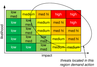
Figure 3: Risk Matrix (example)

In the original ISO/IEC process, the risk value is computed as the product $risk=likelihood\times impact$. It is popular to define a categorical scale for both, the likelihood and the impact (in tabular form explaining what exactly is meant by a “medium likelihood” or a “medium impact”; section 3.8 gives examples). Multiplying the ranks (i.e., category numbers) then gives the risk score and delivers the coloring of the risk matrix as exemplified in Figure 3. Note that loss valuations based on crowd sourcing (expert surveys, detailed in section 3.3) in fact embody both, the impact (as is directly asked for), and the likelihood (as the relative frequency of answers provided by the set of experts polled) in one object. That is, the classical two-dimensional matrix depicted in Figure 3 would boil down to a 1-dimensional list of threats, which can plainly be sorted in $\preceq$-ascending order. Thus, the risk evaluation is even simplified in our setting here. It may nonetheless be advisable to resemble the classical process of risk management a little closer by asking for both, the impact and the likelihood, and construct empirical distributions for both. This may be useful in letting the expert express his beliefs more detailed than just asking for a possibility (and not for a probability too). We revisit this issue later in section 4, after having established the basics of this process first.

In generalizing this classical approach to risk management to a more sophisticated technique based on games and distributions as risk representing objects, our main target in the next section will be modeling the losses as probability distributions, and how to prepare the game theoretic models for the risk treatment phase, when the games are to be solved and “played” in practice. We will exemplify the modeling based on two examples, which are advanced persistent threats (APTs), covered in section 5.1, and social engineering, discussed in section 5.2. Once the cycle in Figure 1 has been completed for once, any repetition entailing another round of risk estimation and risk evaluation can be supported by exactly the same kind of game-theoretic models that were used in the previous risk treatment phase (in fact, the equilibrium strategy enforced as result of the last risk treatment phase is the “do nothing” strategy in the next risk assessment; cf. Table 1). Examples of potentially suitable models are described in the sections to follow. Section 6.3 discusses how to use the game analysis results for effective improvements and control selection.

3 Modelling Losses

The proposed method of risk modeling is here based on non-parametric loss models, for their conservation of information and absence of perhaps difficult to verify assumptions. Nonetheless, actuarial science knows important applications of parametric loss models, which we briefly discuss in the next section.

3.1 Parametric Loss Models

The weight of a distribution’s tails is what makes it (in)appropriate for risk management, where distributions with heavy, fat or long tails are common choices. In the continuous case, extreme value distributions (Gumbel, Frechet or Weibull) are suitable choices, as well as stable distributions. The latter, despite not having analytically expressible densities except for special cases, can nevertheless be ordered upon using sequences of truncations or moment sequences (if they exist) [37].

In the discrete case, the $(a,b,0)$ or $(a,b,1)$ class of distributions may be considered, with a density in the former class being defined recursively as $\Pr(X=k)=\Pr(X=k-1)\cdot(a+\frac{b}{k})$ for $k=1,2,3,\ldots$. The $(a,b,1)$ class is – roughly speaking – the truncated version of an $(a,b,0)$-density excluding the possibility of the event $X=0$. It can be shown that the former class includes exactly three families of distributions, which are Poisson, Binomial and the Negative Binomial distribution.

A general issue with parametric losses is their representation of an arbitrary amount of information by a fixed number of parameters. This inevitably incurs a loss of information, and calls for partly sophisticated methods of parameter fitting or similar. On the contrary, nonparametric losses like (the previously proposed) kernel densities come with the appeal of preserving all information upon which they are constructed, as well as offering the flexibility of allowing for adjustments to model uncertainty in the expert’s answers more explicitly. An example of this will be sketched in section 3.7.

Nonetheless, if a parametric model should be used, then one should bear in mind that risk is intrinsically a latent variable, and the best we can do is relate it to some observable variables. Unfortunately, the usual assumptions on the latent variable being dependent on the hidden variable, so that an inference towards risk is possible, may not directly apply to a risk assessment process. Risk is a property of some general entity, action, intention, or similar. As such, subjective assessments of it are made by humans whose risk perception may be correlated (to a degree that depends on the skill level of the person in the respective regard) but not directly influenced by the true underlying objective value of the risk variable. Still, algorithms like expectation-maximization [27] could (and should) be assessed for the extent to which they can deliver a useful risk model. Indeed, the result of an EM-algorithm being a distribution model over latent variables together with a point estimate on its parameters is a perfectly suitable input for the decision models put forth in the precursor parts of this report.

3.2 Nonparametric Loss Models

Parametric models come at the cost of information loss due to representing the entire data by a (preferably small) set of parameters to the distribution. This is the price for analytic elegance and the ease of many matters related to working with such models practically.

In light of the scarceness and inconsistencies in the data to be expected in a risk management application, we may thus look at nonparametric loss models as a potentially interesting alternative. The method of choice here will follow the proposals made in [37].Specifically, we will start from an empirical distribution compiled from expert interview data, and use a kernel density estimator for our loss model. Moreover, we will focus on discrete risk assessment scales, which lead to discrete (in fact categorical) empirical distributions. For a kernel density estimator in this context, it is somewhat surprising that the literature is unexpectedly thin on discrete kernel density estimates. Besides only a few proposals found in [33, 24, 6], the problem of “good” kernel density estimation seems to be as much of an art (on top of science) as it is in the continuous case. Hence, we will continue defining our own discrete kernel proposal based on Gaussian densities, but postpone the details until later, when we have specified the process of data collection, which obviously goes first.

3.3 Collecting Data from Experts

As for every empirical study, the first step is fixing the details of the scenario about which experts are to be interviewed. In our context, this may entail the identification of a particular threat and related countermeasures. The high level description of a threat, say “unauthorized access to server $X$”, must here be followed by a sequence of possible detailed suggestions on how the respective attack could be mounted. For the aforementioned example, possibilities include the exploitation of (known) vulnerabilities (up to zero-day exploits) in the server itself, social engineering, theft of access credentials, or similar. Normally, each of these possibilities is matched with a respective countermeasure. Risk management standards like ISO 27000 [17, 15] or related ones [4] provide an indispensable source of threats and countermeasures, which can be used in this step.

Abstractly, let us think of this process having brought up a list $PS_{1}$ of countermeasures, opposing a list $PS_{2}$ of possible threat scenarios (the acronym $PS$ means “pure strategy”, as a reminder that we are approaching a game-theoretic model here).

The lists $PS_{1}$ and $PS_{2}$ can be assumed to be quite short (though they must be comprehensive; ideally exhaustive) in practice, and each scenario $(d,a)\in PS_{1}\times PS_{2}$ of “defense ($d$)-vs-attack ($a$)” can be put to its own individual review (not necessarily independent of other scenarios, but the design of questionnaires and the amount of context specification in there is a different and nontrivial story of empirical science not subject of this report).

Remark 3.1 (Simultaneous Occurrences of Multiple Scenarios)

Note that the modeling so far implicitly prescribes the assessment to be done relative to a specific single threat. This restriction can be dropped in presenting the expert a set of threats and explicitly allowing for several of them to occur at the same time. At first glance, this would exponentially enlarge the list $PS_{2}$, this combinatorial explosion can be avoided by allowing the expert to name multiple possible loss categories with different likelihoods. That is, the expert may center the thoughts around a specific threat, but may take further considerations of coincidental other incidents into account in saying that, for example,

• losses of category $x$ are most likely,

• while losses of the larger category $y>x$ remain possible if two or more incidents occur at roughly the same time.

If several such possibilities are uttered, they are most conveniently described by a distribution supported on (at least) the anticipated loss categories $x$ and $y$.

To set up the empirical game theoretic model, let us therefore assume that one scenario $(d_{1},d_{2})$ has been specified in detail, say (for illustration)

$d_{1}$:	perform periodic updates
$d_{2}$:	exploit some software vulnerability

It goes without saying that this specific (example) scenario appears (if at all) in the middle of a real-life APT, as the earlier stages are usually matters of social engineering to make an initial contact and infection. We will go into details of this in section 5.1, and keep our example abstract here only for the sake of illustration.

The goal of data collection is getting a payoff matrix composed from loss distributions that can be used with the game theoretic framework defined in the preceding reports [36, 37].Figure 4 displays the workflow to fill in one cell in the payoff matrix, which is basically done along four steps:

1. Selection and specification of a scenario $(d_{i},d_{j})\in PS_{1}\times PS_{2}$ as a questionnaire presentable to experts (the wording and style of the questions is itself a highly nontrivial matter, and should be done w.r.t. the subsequent implementation strategy for the optimal defense. We will revisit this issue later in section 6.5),

2. Doing an expert survey on the effectiveness of countermeasure $d_{i}$ against attack $d_{j}$. It is crucial for this survey to clearly define at least the following items:

   • the context of the risk assessment (that is, the aspects that are relevant and those that are irrelevant for the risk assessment)

   • a clear definition of the scale in which the risk is quantified (in the style of Table 2 shown in section 3.8 or similar).

3. Collecting as much expert input as possible to define an empirical loss distribution $\hat{L}_{ij}$ over the categories as specified in the survey.

4. Preparing the loss distribution for a subsequent game-theoretic analysis.

The details of step 1 are individually dependent on the application context, i.e., are specific for the system or infrastructure under investigation. This step is recommended to be done according to established standard procedures as described by ISO 27000 or its relatives. Step 2 is a matter of empirical research and questionnaire design. The literature on this is rich, and this task should be left with experienced staff educated in empirical research and statistics. On the technical level, collecting the data is relatively simple, since it is an easy task to set up an online survey, displaying a sequence of questions asking the expert to give her/his risk rating on each described scenario. Things may be even made more efficient by showing the expert the entire matrix, asking to enter a risk assessment in each cell (showing yet another combination of defense and attack), and to leave all fields blank for which there is a lack of domain knowledge or no justified opinion can be expressed.

Step 3 deserves some attention, as this involves an a-priori agreement on the loss categories to be used in the survey. We give details on this in section 3.8.

The final preparation of loss distributions in step 4 is a matter of kernel smoothing, and described in section 3.10.

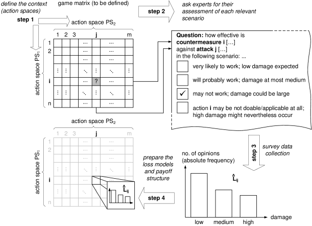
Figure 4: Setting up a Matrix Game with Uncertain Payoffs from Expert Questionnaires

3.4 Refining the Expert Survey

Note that the expert survey – in the form described – only asks for possibilities and not for probabilities. That is, the expert is only questioned to state an expectation of outcome, rather than telling how likely s/he feels it to be. If the survey is refined to ask for a likelihood in addition (as is prescribed in the conventional ISO/IEC risk management standards), then we end up with two probability distributions, one for the impact, the other for the likelihood. A “multiplication” of these two objects, to resemble the usual formula “risk $=$ impact $\times$ likelihood” underlying quantitative risk management, is theoretically possible (as a multiplication of the hyperreal representatives), but not practically meaningful. If the two distributions are available, then a lexicographic comparison of $(impact,likelihood)$ or $(likelihood,impact)$ may be the more reasonable way to go. However, an explicit advantage of the expert surveys and using distributions as representative objects is them embodying both, impact and likelihoods within the same loss distribution object, thus the expert interviews are greatly simplified over the standard risk management process.

3.5 Outlier Elimination

It is important to note that any survey data should be cleaned from outliers, and there has to be a consensus on the treatment of missing values. Either is up to a variety of statistical methods and the particular method should be chosen in light of the given application.

The discussion here is only meant to bring this point to the attention of the reader, and will not go into details of how this could be done.

3.6 Harmonizing Risk Attitudes

After having cleaned outliers, it remains to “harmonize” different kinds of answers depending on the individual personalities and risk attitudes. Persons known to be risk averse will tend to overestimate the risk, while risk seekers will tend to underestimate. It is beyond the scope of this report to discuss concrete methods to correct risk estimates based on a respective classification of the individual, but it is important to bear in mind methods of statistical classification as a potential toolbox to help in this regard.

3.7 Using the Bandwidth Parameter to Model Answer Uncertainty

In some occasions, it may happen that an expert is unsure about whether or not certain circumstances enable certain damages. For example, if the question of whether an incident at one point in the system can cause damage at another point in the system can be answered with “generally no, except for some rare cases”, then the risk assessment related to the incident will have its modal value at a low category, but – due to the possibility of the incident being nonetheless severe – extends the distribution up to the full range of loss categories. The bandwidth parameter of the kernel density estimate can be increased to let the density put more weight on far away categories, or be chosen smaller when the certainty about the assessment (rareness of the incident), is better. In any case, the choice of bandwidth for the kernel density estimates gains another dimension of importance as being a parameter to control/describe the expert’s certainty in the data.

3.8 Defining Risk Assessment Categories

It is crucial (not only for technical reasons) that all loss distributions for all goals in a multi-goal security game must be defined on the same categories. This can be justified by technical but also interpretative reasons:

Technical reason:

the procedure to numerically compute multi-goal security strategies (MGSS) relies on casting the multi-criteria objective function (vector-valued) into a scalar that is a weighted sum. This transformation requires “compatible” objects to be weighted and added (see [37]), which calls for the same underlying scale in all goals.

Interpretation:

comparing the severity of damages in two security goals is only meaningful if the goals are quantified in the same terms. That is, the understanding of, say “high” damage has to be fixed for all goals, and must not be left to a subjective idea that is individual for each expert (otherwise, the outcome of any such assessment is useless). This is especially relevant for non-numeric goals like the reputation of an enterprise, customer trust, or similar.

Especially to address the latter, it appears advisable to underpin the survey/questionnaire by an a priori fixed definition of categories in which the risk assessment shall be made. This can be done in tabular form where each goal is assigned a column, with rows corresponding to the categories, and cell entries describe the meaning of a risk category specifically for each goal. Table 2 shows an example, whereas it must be stressed that the concrete content of the table must be adapted/tailored to the practical situation at hand.

risk category (numerical representative)	loss category
	loss of intellectual property	damage to reputation	harm to customers	…
negligible (1)	$<500$  €	not noticeable	none	…
noticeable (2)	between 500 € and 10.000  €	noticeable loss of customers (product substituted)	inconvenience experienced but no physical damage caused	…
low (3)	$>10.000$  € and 50.000  €	significant loss of customers	damages to customers’ property, but nobody injured	…
medium (4)	$>50.000$ € and 200.000 €	noticeable loss of market share (loss of share value at stock market)	reported and confirmed incidents involving light injuries	…
high (5)	$>200.000$  €  and 1 Mio.  €	potential loss of marked (lead)	reported incidents involving at least one severe injury but with chances of total recovery	…
critical (6)	$>1$ Mio.  €	chances of bankrupt	unrecoverable harm caused to at least one customer	…

Table 2: Potential (Example) Definition of Risk Categories for different Security Goals

Such a table should be displayed together with the survey, to equalize the expert’s individual understandings of the risk categories, and to harmonize the resulting data. The loss categories actually used with the model are simply the integers $1,2,3,\ldots$, noting that the number 0 is precluded as a category (in order not to violate the assumptions made in [36]).

3.9 Using Continuous Scales

If the loss is measured in continuous terms, then a common categorization like outlined above must be replaced by a “meaningful” common (continuous) risk range. The exact definition of “meaningful” must herein be made dependent on the context of the problem, so that all security goals (losses) homogeneously cover the range without being concentrated in disjoint regions. We illustrate the issue with two examples, one showing how it should be done, the other illustrating the problem:

Example 3.2 (well chosen loss range)

Consider two loss variables, with are monetary loss due to theft of intellectual property, and (monetary) investments to protect these assets. Since security is primarily not about making an attack impossible but only about making it non-economic, it can be expected that both losses range in roughly the same numeric region. Formally, let $R_{1},R_{2}$ be the two random loss variables, and let $\varepsilon>0$ be a small value for which we truncate both distributions $F_{1},F_{2}$ at their respective $(1-\varepsilon)$-quantiles, denoted as $q_{(1-\varepsilon)}(F_{i})$ for $i=1,2$. Call the so-obtained loss ranges $I_{1}=[1,q_{(1-\varepsilon)}(F_{1})]$ and $I_{2}=[1,q_{(1-\varepsilon)}(F_{2})]$. If $I_{1}\approx I_{2}$ (i.e., $q_{(1-\varepsilon)}(F_{1})\approx q_{(1-\varepsilon)}(F_{2})$), then we may take the convex hull of $I_{1}\cup I_{2}$ as the common loss range, and be sure that the comparativeness of the two loss variables is retained and reasonable.

Example 3.3 (badly chosen loss range)

Let $R_{1}\sim\mathcal{N}(5,1),R_{2}\sim\mathcal{N}(900,100)$ be two random losses with Gaussian distributions. As before, if the modeler chooses the range as the (convex hull) of the union of both (truncated) ranges at some $(1-\varepsilon)$-quantile, the game may be defined over losses within the common range $[1,1000]$ (for $\varepsilon=0.027$, the range $\mu\pm 3\sigma$ covers $\approx 99.73\%$ of the cases for the Gaussian distribution $\mathcal{N}(\mu,\sigma)$; our cut off here is at $\mu+5\sigma$, and thus covers more than $99.9\%$). Since $R_{2}$, however, assigns most of its mass in the region $[800,1000]$, it will always (at least up to reasonable numerical precision) be $\preceq$-larger than $R_{1}$, so the optimization is pointless.

To avoid situations like sketched in Example 3.3, (at least) two options are available:

1. Rescaling of all loss ranges to a common region. Continuing example 3.3, this would mean replacing $R_{2}$ by $\frac{1}{90}R_{2}\sim\mathcal{N}(10,100/(90^{2}))\approx\mathcal{N}(10,0.012346)$.

2. Defining a common continuous scale with the same intended usage as the discrete categories. That is, if a continuous loss rating is permitted, we may define it within a common interval from $[1,10]$, allowing any value to be picked by the modeler, as long as it is within the range. This may be the method of choice if the modeling interface displays a “slider” where a user can drag the gauge at any position on a continuous scale to express the (subjective) belief about the loss.

3.10 Preparing the Loss Model

In [37], the theoretical possibility of convergence issues in the game’s analysis (by fictitious play) was anticipated, occurring when the loss distributions do not share the same support (this adds to the technical justification stated in the previous section 3.8). Practically, this is highly likely to occur due to missing data. If some categories are simply not being used (either because of an unsuitable definition or because the scale is fine-grained so that not all levels are being used by the experts), then the loss model may be empirically correct, but not useful with a subsequent numeric analysis.

The solution in the continuous case was a kernel smoothing, technically a convolution with a Gaussian density, to extend all loss distributions until a common end of their support (previously called the cutoff point) is reached. We will do the same thing in the discrete case, using a kernel obtained from discretizing the Gaussian distribution. To this end, define $f(x):=(1/\sqrt{2\pi})\exp(-\frac{1}{2}x^{2})$ as the density of a standard normal distribution, and for every $h>0$, define the kernel function $K_{h}:\mathds{Z}\to\mathds{R}$ as

$$K_{h}(n):=\frac{1}{h}\int_{n-\frac{1}{2}}^{n+\frac{1}{2}}f(t/h)dt,$$

where $h$ is the bandwidth parameter (as familiar from continuous kernel density estimates). Obviously, $\sum_{n=-\infty}^{\infty}K_{h}(n)=\frac{1}{h}\int_{-\infty}^{\infty}f(t/h)dt=1$ and $K\geq 0$, so $K$ defines a discrete probability mass function on $\mathds{Z}$. Moreover, it is easy to see that for every $h>0$, the function $K_{h}$ resembles a discrete version of a Gaussian density, so that by letting $h\to 0$, $K_{h}$ degenerates into a discrete Dirac mass,

$$K_{h}(n)\to\left\{\begin{array}[]{ll}1,&\hbox{if }n=0;\\ 0,&\hbox{otherwise.}\end{array}\right.$$ (1)

If we call $\hat{F}_{n}$ a general empirical distribution function (defined on any subset of $\mathds{Z}$) obtained from $n$ data points (answers in the expert survey). The convolution $\hat{F}_{n}\ast K_{h}$ is another distribution function supported on all $\mathds{Z}$, i.e., $(\hat{F}\ast K_{h})(n)>0$ for all $n\in\mathds{Z}$. Moreover, in letting $h\to 0$, we have the pointwise convergence $(\hat{F}\ast K_{h})(n)\to\hat{F}(n)$ for all $n\in\mathds{Z}$, so the estimate is asymptotically correct (note that in contrast to Nadaraja’s theorem, we do not even need to assume a specific speed of decay when letting $h\to 0$). This convergence easily follows from (1). The same result equivalently holds if we replace $f$ by a truncated version $\hat{f}$ thereof (being supported on $[1,a]$ for some integer $a>1$), leading by disretization to the truncated kernel $\hat{K}_{h}$. In the following, we thus consider the smoothed empirical distribution $\hat{F}_{n,h}:=\hat{F}_{n}\ast\hat{K}_{h}$, noting that this also pointwise converges to $\hat{F}$ and that the support (strictly) covers the full interval $[1,a]$. However now, we can make a stronger convergence statement: let $F$ be the (unknown) distribution of the loss assessment, which is approximated by the expert data, which is $F$. We can write

$$\left|\hat{F}_{n,h}-\hat{F}_{n}+\hat{F}_{n}-F\right|\leq\left|\hat{F}_{n,h}-\hat{F}_{n}\right|+\left|\hat{F}_{n}-F\right|$$ (2)

To the first term, we can apply a uniform bound thanks to the supports of $\hat{F}_{n,h}$ and $\hat{F}_{n}$ being all finite, which is

$$\sup\left|\hat{F}_{n,h}-\hat{F}_{n}\right|\to 0\quad\text{ as }\quad h\to 0,$$

as is an easy consequence of the equivalence of all norms on $\mathds{R}$. The other term in (2), we can apply Glivenko-Cantelli’s theorem to conclude the convergence

$$\sup\left|\hat{F}_{n}-F\right|\to 0,\quad\text{ as }\quad n\to\infty,$$

so that $\sup\left|\hat{F}_{n,h}-F\right|\to 0$ in the limit $h\to 0$ and $n\to\infty$. Note that this argument is only good for plausibility of our approach, but cannot be taken as a proof of correctness, since practically, it still relies on an infinitude of data, which – more crucially – must be objectively sampled from the real loss variable (having the distribution $F$).

On the bright side, however, the proposed smoothing enjoys a nice intuitive justification as accounting for uncertainty in the assessment.

Example 3.4

Suppose an expert utters the opinion that, on a scale from 1 to 5, the risk is 3. Despite that a middle assessment is an implicit statement of uncertainty already, there statement “the risk score is 3” is not equivalent to the statement that the risk cannot be anything else. In other words, there may be admitted chances of the damage being higher or lower than the average told by the expert. To express such uncertainty more detailed, the expert may admit possible outcomes on the entire range $1,\ldots,5$, with the initial assessment being just the most confident outcome.

Of course, it will not be feasible to ask experts to provide entire probability distributions over a scoring scale, but the smoothing of the empirical distribution by convolution with $K_{h}$ achieves the same thing. Viewing $K_{h}$ as a set of weights associated with all possibilities around the mean value $x$, the expert assessment $x\in\mathds{Z}$ receives the maximal weight (as being the modal value of $K_{h}$), whereas all other possibilities receive a nonzero weight that decays with the distance to the value $x$. Graphically, this process thus “fills” all empty bins in the empirical histogram (say, if a category has never been assigned during the expert survey), and additionally extends the distribution up to the full and identical support for all loss distributions. Hence, besides satisfying the technical constraints imposed, the smoothing naturally accounts for the uncertainty in the assessment; the lower the parameter $h$ is, the more confident we are in the assessment (i.e., the closer the smoothed approximation $\hat{F}_{n,h}$ approaches $\hat{F}_{n}$). Figure 5 displays an example of the original empirical histogram (Figure 5c), and its smoothed version with $h=1$, having its gaps filled in by the superposition of smoothing kernels (expressing the uncertainty around the modal values given in Figure 5c), and another smoothed version of the histogram with a much smaller bandwidth parameter $h=0.25$. This plot visually illustrates (confirms) the formal claim of convergence as stated previously.

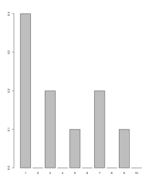
(a) Original empirical histogram

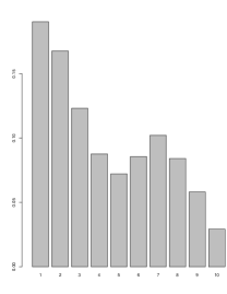
(b) Smoothing with $h=1$

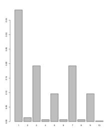
(c) Smoothing with $h=0.25$

Figure 5: Effect of smoothing the histogram to fill empty categories and extend the support

The quality of the kernel density estimation, as in general with this nonparameteric method, is the art of choosing the bandwidth parameter $h$. Various rules of thumb (e.g., Silverman’s rule [43]) or cross-validation techniques may be applied. Since there is no generally “best” way to choose this parameter depending on the information at hand, we refer to the literature on nonparametric statistics for concrete methods [49, 47, 8].

4 Risk Prioritization

Let us assume that a total of m threats $T_{1},\ldots,T_{m}$ has been identified. If, say $n$, experts provide their input on the impact and likelihoods (both artefacts obtained by surveys as outlined in section 3.3), then it is a simple matter to compile an empirical histogram (a distribution $F_{I}$) for the impact and another empirical histogram (a distribution $F_{L}$) for the likelihood. In doing so for every threat $T_{1},\ldots,T_{m}$, we end up with $2m$ such distributions, which we denote here as $F_{(}k,I),F_{(}k,L)$ for the $k$-th threat $T_{k}$ in the list. To resemble the risk matrix familiar from the standard process of risk management, we can use the $\preceq$-ordering on the distributions (remember that it is a total order), to separately sort the threats $T_{1},\ldots,T_{m}$ in ascending $\preceq$-order according to their impact and likelihood. This gives two lists, in which each threat gets a rank assigned among the total of $m$ threats, say the $k$-th threat has rank $r_{i}$ on the impact ranking and position $r_{j}$ on the likelihood ranking. The risk matrix familiar from the ISO processes (cf. Figure 3) is then re-established by placing each threat into a 2D-coordinate system with the $x$-coordinate being the rank on the impact scale and the $y$-coordinate being the rank on the likelihood scale. This puts each threat to a particular position on the grid, and we may then proceed “as usual” by coloring the area as we would do for a normal risk matrix. Likewise, the “critical region” can be defined as the area inside which threats fall that need to be addressed by the subsequent risk management process. Figure 6 displays an example.

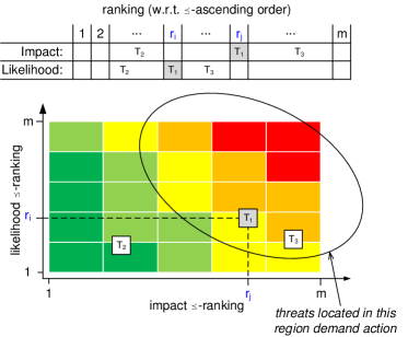
Figure 6: Risk Matrix using $\preceq$-Orderings

The main difference to the standard risk matrix is herein twofold:

1. While a standard risk matrix has axes scaled in categories, the so adapted risk matrix has axes scaled in ranks that go from 1 to the total number $m$ of threats.

2. The consensus problem of assigning a threat a single quantification in terms of likelihood and impact is avoided. Since many experts can utter disagreeing opinions, all of which go into the impact- and likelihood-distributions $F_{I}$ and $F_{L}$ with equal importance. The total ordering $\preceq$ then assures somewhat like a “base-democratic” ranking, since one threat outranks the other in the $\preceq$-ordering, if more people classify the impact, respectively the likelihood, as high (see [37] for the full detailed effect of this ordering).

If the assessment considers multiple criteria, say, if the impact is not only measured in money but also in reputation, then the respective assessments are made separately (not necessarily independently) from one another. For the example of budget-impact and reputation impact, we could think of the one distribution $F_{I}$ as being replaced by two new distributions $F_{BI}$ and $F_{RI}$ (for budget and reputation). Likewise, if two threats have assessments in these terms, given as $F_{(BI,1)},F_{(BI,2)}$ and $F_{(RI,1)},F_{(RI,2)}$, then we ought to rank the two in terms of two criteria. A canonical way of doing that is offered by defining a game with two goals (“budget” and “impact”), and using one (dummy) strategy for player 1, and letting the two threats being the strategies for the opponent (player 2). It is, however, important to stress that we cannot directly go ahead and set up a multi-criteria $(1\times n)$-game to get the most severe threat via an equilibrium, since the gameplay is defined to be among $n+1$ players, where each opponent (corresponding to a goal) plays independently of all others. The equilibrium would then return a worst-case threat identified per goal, which is possibly not what we seek here for a multi-criteria risk optimization. The theory, however, remains applicable when the game is reduced to a two-player $(1\times n)$ game with scalar(ized) payoffs per player. In that case, the equilibrium is necessarily pure and indicates the worst case threat for player 1. The R package implements this method in a designated procedure preference:

# ranking if there is only one goal (say, FBI1, vs. FBI2)
> preference(FBI1, FBI2)
2 # this means that the second parameter (FBI1) is preferable

# ranking, if there are multiple goals (of equal importance)
> preference(list(FBI1, FRI1), list(FBI2, FRI2))

# Let us assign twice as high priority to the "reputation"
# goal by supplying the parameter weight=c(1,2), i.e. "goal" has
# priority 1, and "reputation" has the (double) priority 2.
> preference(list(FBI1, FRI1), list(FBI2, FRI2), weights=c(1,2))

The results directly gives the desired ranking by telling that either the first (output “1”) or second (output “2”) threat is less severe; if the function returns zero, then the distributions are identical and the decision is indifferent. For three or more threats, the procedure can be repeated pairwise to rank a whole set of threats in the way as described above.

5 Examples of Game-Theoretic Modeling

5.1 Modeling APTs

The investigation of many examples of advanced persistent threats (APTs) reported in the past reveal a common structure underlying an APT, even though the details thereof may be highly different. Quoting the taxonomy of [7], an APT roughly proceeds along the following steps:

1. Initial infection:

   1. reconnaissance: information gathering,

   2. development: design of a made to measure malware,

   3. weaponization: preparing the trojan and droppers,

   4. delivery: transmission into the victim infrastructure, e.g., by a phishing email, or similar.

2. Learning and propagation: repeated sequence of

   1. exploitation: to get deeper into the system

   2. installation: to leave artifacts and backdoors for an easy return later, and destroy footprints of the attack

3. Damage:

   1. command and control: interaction with the victim system’s compromised resources via previously left artifacts

   2. actions on the target: causing the actual damage

The specific actions taken in each of these phases depend on the target infrastructure and no general description is possible due to the diversity of such infrastructures. However, specific examples can be “read off” reported prominent incidents, such as including Stuxnet [10], Duqu [2], Flame [28], and Aurora [23]. A common element in all these appears to be the human factor, which we discuss separately in section 5.2.

Game theory has been applied in various ways to model attacks and cyber risks [25, 9, 50] and proposals (independent of game theory) include moving target defenses [19, 18], trust mechanisms [48], and defense-in-depth techniques [30]. Here, we will review a recent proposal to model APTs as a sequence of games, each of which is tailored to the specific nature and details of the respective phase.

That is, an APT usually begins with a harmlessly looking email or “lost” USB stick, on which malware enters the system. Alas, nowadays attackers have joint forces into an entire illegal business sector covering the entire supply chain of cyber crime in a spectrum of independently offered services (often referred to as “cybercrime as a service” in alignment to cloud computing terminology). This means that the person identifying a weakness is not necessarily the same who is writing the exploit for it. Likewise, the author of the exploit kit is not necessarily applying it anywhere, but merely sells it to the actual attacker. Similarly, infections with malware are not automatically intended to cause immediate damage. The term “botnet-as-a-service” describes the business model of infecting a large number of machines and offering to deploy malware on these zombies upon request and for a (smaller or larger) fee. In this way, the attacker can simply “buy” access to a potentially large number of infected machines instantly. For the victim, this has the unpleasant effect of the infection remaining stealthy and inactive, until some time later, when the outbreaks causes noticeable damage. At this time, however, it is most likely that no connection between a past email and the current incident is recognized. The exact time window between an infection and its activity is also dependent on the technical countermeasures adopted in the specific company. For example, signature-based malware recognition (like classical anti-virus software used to work) may take a couple of days until the malware is recognized as such and the respective signature is shipped with the next update. On the contrary, cloud based malware detection that is based on recognizing a huge lot of “identical” email (attachments) suddenly flowing through the internet can have a much shorter time (even a few hours) until a malware is suspected and classified. So, the time window between the infection and the exploit may, in some cases, be closed quite fast (by a good malware recognition system).

To model a so-structured APT in terms of games, the first step is listing all potential ways into the system, such as include (but are not limited to):

• (spear) phishing, whaling,

• waterholing,

• tailgating,

• etc.

The entirety of these possibilities makes up the set of strategies $PS_{2}$ for the attacker. Typically, an entry in $PS_{2}$ is thus not constrained to have a specific form or structure (in particular, an element $x\in PS_{2}$ is not a purely mathematical object but rather a description of how an attack would be launched according to this particular strategy $x$).

In a different view, $PS_{2}$ can be considered as a list of threats, to which corresponding countermeasures can be defined (appealing to catalogues found in standards like ISO 27000, etc.). The list of countermeasures is $PS_{1}$.

Note that $PS_{1}$ and $PS_{2}$ should be defined bearing in mind the steps and structure of the first phase of the APT, which comprises information gathering, development, weaponization and delivery. Consequently, example defense measures in $PS_{1}$ may relate to periodic (and random) re-configurations of the system in order to thwart the attacker’s respective next steps, either by invalidating so-far collected information or by removing malware by coincidence, say if a computer is reinstalled or privileges of the victim user have changed (were revoked).

In any case, let the game describing the initial infection be a matrix game $G_{1}$ (where the subscript is a reminder of this being the first phase of the APT). It appears fair to let this be a matrix game (static and repeated), since if the game is expectedly repeated either in case of an attack failed, or to infect further parts of the system, if an attack was successful.

Let the equilibrium computed for the infection game $G_{1}$ be the pair of distributions $(F_{1}^{*},F_{2}^{*}$), where the optimal defense against the initial infection is the distribution $F_{1}^{*}$ (the distribution $F_{2}^{*}$, more specifically, its probability mass function can be taken as a non-unique indicator set of neuralgic points in the infrastructure).

To model the next phase of learning and propagation, we divide the (physical) infrastructure in stages that the adversary needs to reach one by one in order to get to the inner target asset. If the infrastructure is a network graph $G(V,E)$, then the target asset may be a(ny) fixed node $v_{0}\in V$, and the $i$-th stage can (but does not need to) be defined as the set of nodes at distance $i$ to the node $v_{0}$. That is, the stages are “concentric circles” around the asset, and on each stage, the adversary plays a (different) game to get to the next stage. A single such stage is penetrated by the aforementioned steps of exploitation and installation, continuing with exploitation again on the next stage (only in a different setting there). This modeling is practically supported by topological vulnerability analysis (TVA), which can cook up an attack graph for an infrastructure. In the following, we will illustrate our thoughts based on Example 5.1.

Example 5.1 (based on [44]; see also [40])

Consider a system as shown in Figure 7b, composed from three devices, with various ports opened and services enabled.

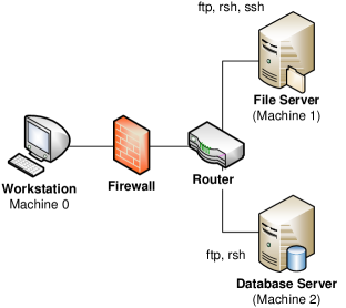
(a) Example Infrastructure [44]

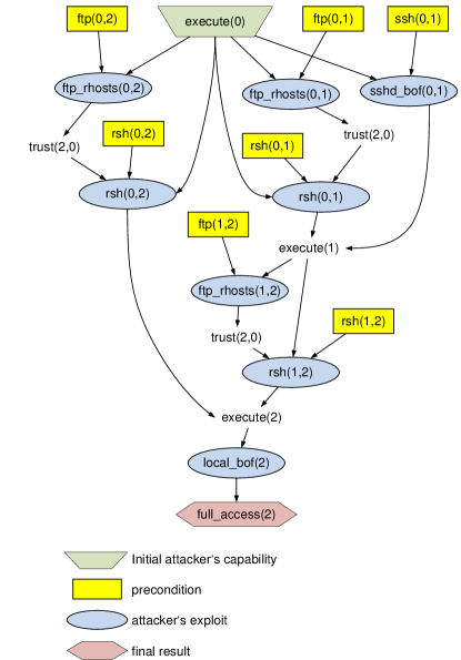
(b) Example Attack Graph [44]

Figure 7: Topological Vulnerability Analysis Example

Based on this information, the attacker can consider several exploits, such as:

• FTP- or RSH-connections from a node x to a remote host y, hereafter denoted as ftp_rhosts(x,y), and rsh(x,y), respectively.

• a secure shell buffer overflow at node y, remotely initiated from node x, hereafter denoted as sshd_bof(x,y).

• local buffer overflows in node x, hereafter denoted as local_bof(x).

Each of these may establish a trust relation between two nodes x and y, which we denote as trust(x,y). The list of attack strategies to penetrate all the stages until full_access to machine 2 is a matter of plain path enumeration in the attack graph, whose results are shown in table 4.

Table 3: APT scenarios (adversary’s action set $PS_{2}$, based on Figure 7)

1	execute(0) $\to$ ftp_rhosts(0,1) $\to$ rsh(0,1) $\to$ ftp_rhosts(1,2) $\to$ sshd_bof(0,1) $\to$ rsh(1,2) $\to$ local_bof(2) $\to$ full_access(2)
2	execute(0) $\to$ ftp_rhosts(0,1) $\to$ rsh(0,1) $\to$ rsh(1,2) $\to$ local_bof(2) $\to$ full_access(2)
3	execute(0) $\to$ ftp_rhosts(0,2) $\to$ rsh(0,2) $\to$ local_bof(2) $\to$ full_access(2)
4	execute(0) $\to$ rsh(0,1) $\to$ ftp_rhosts(1,2) $\to$ sshd_bof(0,1) $\to$ rsh(1,2) $\to$ local_bof(2) $\to$ full_access(2)
5	execute(0) $\to$ rsh(0,1) $\to$ rsh(1,2) $\to$ local_bof(2) $\to$ full_access(2)
6	execute(0) $\to$ rsh(0,2) $\to$ local_bof(2) $\to$ full_access(2)
7	execute(0) $\to$ sshd_bof(0,1) $\to$ ftp_rhosts(1,2) $\to$ rsh(0,1) $\to$ rsh(1,2) $\to$ local_bof(2) $\to$ full_access(2)
8	execute(0) $\to$ sshd_bof(0,1) $\to$ rsh(1,2) $\to$ local_bof(2) $\to$ full_access(2)

A selection of respective countermeasures is given in table 4.

Table 4: Security controls (selection) – subset of $PS_{1}$

countermeasure	comment
deactivation of services (FTP, RSH, SSH)	these may not be permanently disabled, but could be temporarily turned off or be requested on demand (provided that either is feasible in the organizational structure and its workflows)
software patches	this may catch known vulnerabilities (but not necessarily all of them), but can be done only if a patch is currently available
reinstalling entire machines	this surely removes all unknown malware but comes at the cost of a temporary outage of a machine (thus, causing potential trouble with the overall system services)
organizational precautions	for example, repeated security training for the employees. These may also have only a temporary effect, since the security awareness is raised during the training, but the effect decays over time, which makes a repetition of the training necessary to have a permanent effect.

The game to model the penetration can then be defined per stage by defining the machines 0, 1 and 2 as stages, where machine 2 is the inner assert (node $v_{0}$ in our previous wording), and a stage is the game played to establish a trust relation between a machine at distance $i$ and one at distance $i-1$ to machine 2.

In the (quite simple) infrastructure of Figure 7a, the stages would thus be:

• stage 1 (distance 1 to machine 2): {router}

• stage 2 (distance 2 to machine 2): {file server (machine 1), firewall}

• stage 3 (distance 3 to machine 2): {workstation (machine 0)}

The game played at stage 3, accordingly, has strategies equal to all exploits that can be mounted on the workstation (machine 0), which can be read off the TVA attack tree (Figure 7b) as $PS_{2}=\{$ftp_rhosts(0,1), ftp_rhosts(0,1), sshd_bot(0,1)}. The corresponding set $PS_{1}$ comprises all countermeasures that can be implemented (such as virus checks, temporary disabling of services, but also non-technical ones like repeated security training, etc.). The strategy spaces $PS_{1}$ and $PS_{2}$ identified in this way then define the shape of the respective 3rd stage game $G_{3}$, whose payoff structure is to be defined following the procedure outlined in section 3.3; Figure 4.

The games for the other stages are constructed analogously.

Given a game for each stage, we can connect them into an overall model for phase two of the APT by adopting a high level perspective. In each stage, the adversary has basically two options, which are:

1. penetrate: this means launching an attack as identified based on previously gathered information (cf. example 5.1), or

2. stay, to collect more information while remaining stealthy $\to$ learning.

Both options can be modeled using their own (distinct) game models, and the connection between the games over all stages is established by considering that in the $n$-th stage game (whether we go for penetrating or staying), the outcome is one of the following:

• if the attacker decides to penetrate, then

  • it may succeed, in which case it enters game $G_{n-1}$, or

  • it may fail, in which case it has to repeat game $G_{n}$ once more.

• if the attacker decides to stay, then

  • it may succeed and gain further information, but this leaves the attacker in this stage $n$,

  • it may fail, in which case the overall game terminates, and the entire investment of the attacker is lost (we model this as a negative gain for the attacker).

Likewise, the defender has the option of defending (without any guarantee of the defense being successful), or not defending. The latter strategy is implicitly played whenever the defender “pauses” in its defense, say, if the security guard is being sent elsewhere and misses the attack by this unfortunate coincidence. In any case, “do not defend” is never a dominating strategy and occurs only due to resource limitations and the inability to defend everywhere at all times against everything.

Writing $I(n)$ for the payoff (to the adversary) in the $n$-th stage, the above modeling yields a $2\times 2$ zero-sum matrix game structured as shown in Figure 8 (cf. [41]). In this model, we have additional quantities $p(n)$ and $q(n)$ that depend on the current stage, and quantify the likelihood for each action to be successful. These values can be either defined directly, or themselves be derived as saddle point values of classical 0-1-valued matrix games in each stage (in this case, the risk assessment is done in binary terms only asking the expert for whether or not the attack will be successful).

	penetrate	stay
defend	$p(n)\cdot I(n-1)+(1-p(n))\cdot I(n)$	$q(n)\cdot I(n)+(1-q(n))\cdot(-I(n))$
do not defend	$I(n-1)$	$I(n)$

Figure 8: Sequential 2-Player Game Model for Advanced Persistent Threats

It is reasonable to assume a circular structure in this game (cf. also [1]), which amounts to a single unique equilibrium, for the following reasons:

• if “defend” is a dominating (row) strategy, then either “stay” or “penetrate” will complete this into an equilibrium, and there is nothing to be optimized by game theory here on this (higher) level.

• if “do not defend” is a dominating (row) strategy, then there is no need to do any active security here, as the infrastructure is already secure anyway.

• if “penetrate” is a dominating (column) strategy, then the obvious best choice is to defend, which again degenerates the game into a trivial matter.

• if “stay” would be a dominating (column) strategy, then there is no need to defend anything, since the attacker is not trying to get to the asset anyway.

In any case, it is a simple (yet laborious) matter of working out the game matrix for each stage, and determine an equilibrium for it (say, using fictitious play as described in [37]). The particular equilibrium obtained for the $n$-th stage is the distribution $I(n)$, telling us the distribution of damage in that stage, accompanied by optimal defenses in this stage (obtained from the $2\times 2$ game and the inner sub-games played for penetration and to collect information during a stay).

Concluding the idea, the decomposition of the learning-and-penetration phase in the APT life cycle into stages and corresponding games played therein delivers an in-depth defense action plan (individual randomized defense actions being taken on each part in the infrastructure), as well as a higher-level risk assessment $I(1),I(2),\ldots$ that refers to each stage. The distribution $I(n)$ for the $n$-th such stage then indicates the likelihood of damage suffered at the $n$-th “protective layer” around the asset of interest.

The final game modeling the Damage-phase of the APT can then be defined similar to the initial infection game $G_{1}$, as the attacker may simply try and retry causing damage. The process and steps to identify possible actions and countermeasures must again be supported by special purpose (and application specific) tools and expertise, but the game theoretic treatment and computation of risk metrics remains the same. Thus, we will not repeat the details here.

A Static Game Model for the Penetration Phase

In a more simplified view towards a substitute of the sequential phase two game, a static game model can be considered as an alternative (being easier to model and more efficient to analyze computationally). This simplification is bought at the cost of getting a more coarse-grained model, since the attack and defense strategies are defined more “high-level” and not specific for each stage in the graph representation (of the infrastructure or the attack tree).

As before, we can think of the attacker working its way through the stages, while occasionally being sent back or kicked out if a security officer (perhaps unknowingly) closes some of the backdoors established previously. The pure strategy set $PS_{1}$ for the defender is thus the set of all nodes/components in the system on which spot checks (e.g., malware scans, configuration changes, updates, patches, etc.) can be done. Different to the per-stage game modeling from before, the defenses now correspond to high-level attack strategies $PS_{2}$ that describe only techniques but are not specifically tailored to a particular machine. That is, $PS_{2}$ would be composed from a more generic set of threats like

• buffer overflow exploits,

• cross-site scripting,

• code injections,

• etc.,

but unlike in Example 5.1, these attacks would not be considered on specific machines. Rather, the attack scenario is described as a general code injection that may be tried on any machine in the network (if possible). The description of the attack/defense scenario, as well as the possibilities to consider for a risk assessment may be more complex in this kind of modeling, as Example 5.2 shall illustrate.

Example 5.2

The expert survey would ask something like:

What is the expected damage if an attacker attempts a code injection attack in our infrastructure, while machine 1 (see Figure 7a) is being re-installed at roughly the same time.

To answer this question towards a loss estimate, the expert may consider the following aspects:

• Which machines could be vulnerable to such an attack (say, which of them are accessible by a web interface or maybe have an insufficient patch level, etc.)

• Depending on which machine is attacked, the damage may be more or less (thus allowing the expert to utter multiple possibilities; substantiating the construction of a categorial loss distribution once again).

• Depending on where the spot check is done (say, on machine 1 in Example 5.1), three cases are possible:

  • Machine 1 has so far not been reached by the attacker (more precisely the attack path), so the reinstallation has no effect on the APT at this stage.

  • Machine 1 is exactly the one currently targeted by the attacker. This may render the results of the APT learning phase on this machine useless, since the configuration has changed. Consequently, the attacker is sent back one stage and has to restart learning from here.

  • Machine 1 has already been infected with malware, so that the adversary’s backdoor path goes through it. In that case, the attacker’s secret backdoor may be closed by the reinstallment and the attacker is again sent back to a previous stage.

Since there is uncertainty on where the attack may be mounted, and also on the current position of the adversary, the expert may utter several possibilities in one of two ways:

• Tell about a set of possibilities, expressing the likelihood for each of them individually. For example, the expert may say something about the most likely outcome, but in addition also say that more or less extreme results are possible with certain other likelihoods.

• Give a most likely outcome $r$, and express the uncertainty about it: this in fact corresponds to the aforementioned kernel density smoothing, since the uncertain variation around the most likely value (as expressed by the expert) may be well expressed by a bell-shaped curve centered around the value $r$. This is nothing else than a kernel density, where the uncertainty is “quantified” by the parameter $h$.

In repeating the procedure exemplified in Example 5.2 for each (high-level) defense/attack scenario $(d_{i},a_{j})\in PS_{1}\times PS_{2}$, we end up with a standard matrix game defined with probability-distribution valued payoffs, which are now defined not on the risk categories, but on the graph theoretic distances, or more specifically, the stages between the initial infection and the inner asset. Picking up Example 5.1, there are three stages which the attacker has to proceed through, and the loss distribution defined per defense/attack assigns likelihoods to each of these stages; Figure 9 displays an example. The game-theoretic optimization then goes for pushing the probability mass towards “more remote” nodes in the network (or attack graph). That is, we will try maximizing the distance between the attacker and the asset, measured as the number of hops ($=$ stages in our wording) that need to be taken to reach the goal. The stage numbering should, for consistency with the minimization, be increasing from 1 up to the stage where the asset is, i.e., stage 1 should comprise the outermost perimeter, followed by the adjacent inner nodes, until stage $N>1$ being the set of final nodes adjacent to the target asset.

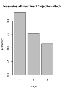
Figure 9: Example of loss distribution on stages (phase 2 of an APT)

5.2 Modeling Social Engineering

Social engineering is a good example of a case where the distribution-valued game-theoretic framework perfectly fits. Since there is hardly any technical countermeasure against such attacks, and the exploits are based on psychological principles of human behavior, there is also an element of “forgetting” that makes security awareness decay over time. For this reason, security training, information campaigns and similar must be repeated from time to time, and there is never a guarantee that any of these precautions has any or even durable effect. Both of these reasons render matrix games with distribution-valued payoffs into a nice model, since:

• the necessity of repeating social engineering awareness training corresponds with the modeling assumption on the matrix game to be repeated.

• the finiteness of matrix games corresponds to the limited set of possible countermeasures known against such attacks. That is, we cannot ask an employee just to become “creative” in how social engineering may be detected, and the best we can hope for is a feasibly small set of recommendations that a person can remember to avoid falling victim to social engineering.

• the inevitable element of human error renders the outcome of a social engineering scenario in any case up to randomness. Hence, our specification as a distribution-valued matrix game appears as a good fit, as it allows us to classify social engineering countermeasures as being “variably effective” (taking into account the differences in people’s personality, daily mood, current workload, technical skills, time since the last security awareness training, and many more).

For a pure model of social engineering attack/defense scenarios, the questionnaire outlined in section 3.3 may be adapted to poll people about their awareness against social engineering, describing the particular attack scenario in the description of the question, and asking the employee on how he/she would behave in this scenario. The results then equally well compile into the sought loss distributions, if each answer in the multiple-choice survey has a background association with a predefined loss category (cf. section 3.8).

A different approach to account for social engineering when it comes to loss distributions is considering these attacks as methods to establish the initial infection in an APT model as outlined in section 5.1. Here, we would include social engineering techniques in the attacker’s strategy space $PS_{2}$, and the specification of the respective success rates can be done using the same kind of survey as before. The resulting game then already models the first phase of an APT infection, in giving the probability for a social engineering attack to succeed under the given security awareness campaign (which is a mixed strategy over $PS_{1}$ in the sense of repeated randomly selected trainings, information broadcast, etc.).

The second phase of the APT, the penetration, can as well use social engineering techniques to overcome barriers within the system. Suppose that a subnetwork, for security reasons, does not have any physical or logical connection to the outside or any other intranet within the company. Then a malware can jump over this physical separation by a bring-your-own-device incident. That is, if the malware gets into the system by someone connecting a virulent USB stick to the inner separated network, the infection has effectively overcome the logical separation. Even more, this scenario may start from within the company’s perimeter, since the infection of the USB stick may indeed happen on an employees’ computer, which has a connection to the internet and got infected in the first phase.

The respective loss distributions associated with such an infection outbreak can effectively be constructed by simulation, as is eloquently outlined in [22]. We leave the details aside here.

6 Working with Game-Theoretic Risk Measures

The description in the following is based on the previous explanations about the model, and therefore only discusses practical matters of choosing the parameters and hints on how to interpret the results. A description on how to do the calculations with aid of the R statistical software suite is given in section 6.4.

6.1 Choosing the Cutoff Point

So far, we mentioned the necessity of truncating distributions only as a technical matter of assuring convergence. As such, the point $a>1$ at which the payoff distributions are truncated (for a compact support) also influences the outcome of the game, since the equilibria depend on it. Indeed, the practical choice of $a$ can be made in light of how $a$ determines the $\preceq$-relation among the payoffs. Informally, Lemma 4.4 in [37] tells that $\preceq$ is decided based on how the payoff densities behave in a right neighborhood of $a$. That is, the setting of the value $a$ controls the range in which damages are considered as relevant for $\preceq$, whereas damages far lower than $a$ become less and less relevant for the $\preceq$-relation. This means that the choice of $a$ can be made to implement a risk prioritization in the model in a sense that is perhaps best illustrated by an example (cf. also [38] for a related yet different illustration):

Example 6.1

Suppose an enterprise has backup capacities to bear losses less than $50.000~{}€$. Then, we may set the truncation point $a:=50.000$, so that the entire probability mass assigned to damages $>a$ is “squeezed” underneath the distribution on the interval $[1,a]$. Consequently, if a loss model $F_{1}$ admits highly likely losses $>50.000~{}€$ (i.e., has in that sense a fat tail) will result in a higher value of $f_{1}(a)$ than maybe the alternative loss distribution $F_{2}$, assigning smaller likelihood to such incidents (and in turn coming out with a smaller density $f_{2}(a)$). Thus, $f_{1}(a)>f_{2}(a)$ will make $F_{2}$ $\preceq$-preferable over $F_{1}$ [37].

The dependence of the resulting equilibrium is best visualized by taking another example of a $2\times 2$-game with continuous payoff distributions as shown in Figure 10. Taking the cutoff point $a=10$ results in a pure equilibrium $(\bm{x}^{*},\bm{y}^{*})=((1,0),(1,0))$, while truncating the distributions at $a=6$ changes the equilibrium into a mixed one, namely, $(\bm{x}^{*},\bm{y}^{*})=((0.751,0.249),(0.531,0.469))$. Both of these have been obtained using fictitious play as described in [37] taking 1000 iterations.

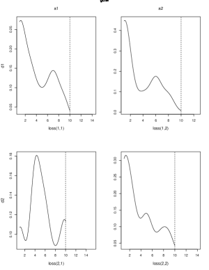
(a) Cutoff at $a=10$

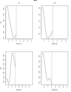
(b) Cutoff at $a=6$

Figure 10: Payoff structures with different cutoff points

6.2 Interpretation and Meaning of Equilibria

The difference in the equilibria computed for the previous examples is immediately understood by looking at the way how $\preceq$ depends on the truncated distribution’s tails (cf. [36, 37]): if the cutoff point $a$ is chosen so large that the likelihoods assigned to events around $a$ are approximately equal, then there is no point in frequently switching strategies for either player, since the outcome under any of the four scenarios admitted by the example $2\times 2$-game is roughly the same. Hence, the equilibrium is “purified” by the choice of the cutoff point. Conversely, if the cutoff point $a$ is chosen so that the masses that accumulate around it are significantly different, then mixed equilibria may arise.

This has a twofold and partly positive consequence for the risk manager, since:

• the practical choice of the cutoff point $a$ can be made to mark the region in which risks are considered as relevant. That is, if there is an agreement that damages beyond some threshold value are highly relevant, while everything below it is only of secondary interest, then the cutoff point $a$ can be set to exactly this threshold value. More importantly, any such setting is not even to be taken as sharp, since what determines the $\preceq$-relation is the left neighborhood of $a$, so the transition from the domain of acceptable risks to the area of critical risks is somewhat smooth.

  For example, if the risk management is done in terms of a CVSS scoring, then the risk manager may fix the convention of not caring about vulnerability scores in the range around 2, but certainly action is demanded for scores above $7$. In that case, we would set the cutoff point to $a=7$, in which case the game optimization focuses on scorings of 7 or (slightly) less, while the region around scores of $2$ becomes relevant only upon equiprobable ratings of all defense actions on the range $(2,7]$.

  This effect holds in general and is not limited to the example games here. In fact, the cutoff point creates a qualitative difference to conventional optimization, where the numeric magnitude of the goal function is irrelevant for the maximization. This may not practically be the case, but can be accounted for by setting the cutoff point accordingly.

• An equilibrium must in any case be interpreted relative to the cutoff point. If $a$ can reasonably/meaningfully be chosen so that pure (or approximately pure) equilibria arise, then these greatly ease matters of playing the equilibrium. That is, if the risk prioritization results in almost all actions ending up with approximately equal likelihoods in the relevant neighborhood of $a$, then practically playing the optimal behavior is easy, since the best response is no longer randomized.

Risk vs. Goal Prioritization:

The role of the cutoff point in risk prioritization must be distinguished from the role of the weights (discussed in [37, Sec.4.5.1]) assigned to reflect the priorities of different goals in an MGSS. In fact, this is a different degree of freedom, and goal priorities (the weights $\alpha_{i}$ for $i=1,2,\ldots,d$ goals can be chosen independently of the cutoff parameter $a$).

6.3 Optimizing an Infrastructure’s Resilience (Risk Treatment)

If the line between threats that need to be addressed and those that can be left aside (for the moment) has been drawn, i.e., the risk evaluation phase is completed, the risk treatment concerns the selection of controls to mitigate the threats.

Given one or more threats to be addressed, risk treatment is about selecting controls against them. The particular selection of controls and resource allocation is a matter of optimization, and this is where game theory comes into play. Specifically, it helps to determine the optimal style of implementing controls towards minimizing the risks. The procedure, on a high level, is defining a game matrix that has a list $PS_{2}$ of adversary’s actions (typically the threat or a set of threats to be considered), and another list $PS_{1}$ of controls that address the threats. Note that the setup of the game matrix, specifically the definition of $PS_{1}$ and $PS_{2}$ should be made with care: it may well be the case that some controls in $PS_{1}$ may not address certain threats in $PS_{2}$ and vice versa. For example, if we have the countermeasures

• $d_{1}\in PS_{1}$: “installing an intrusion detection system”

• $d_{2}\in PS_{1}$: “install more fire extinguishers”

And the threat list $PS_{2}$ includes

• $T_{1}\in PS_{2}$: fire outbreak

• $T_{2}\in PS_{2}$: hacking attack

Then it is obvious that $d_{1}$ is pointless against $T_{1}$ and $d_{2}$ has no mitigating effect on $T_{2}$. In such cases, one may consider a clustering of threats and controls based on their mutual relevance. This amounts to selecting specific controls against specific threats, and allows an optimized control selection “per threat” or “threat group” (if a control is effective against more than one threat). Once the lists $PS_{1}$ and $PS_{2}$ have been specified, it pays to sub-classify the actions in $PS_{1}$, as there are:

Static controls:

these have a permanent effect in being a change to the system structure. Their selection must be based on the goal of finding the minimal set of controls that covers the maximal spectrum of threats. If several candidate controls are available, then the problem is “game-theoretic” in the sense of being a humble optimization for the defender having $n$ strategies against a specific single strategy of the attacker (that is the threat to be mitigated). If all threats shall be mitigated at the same time, then the problem of control selection can be set up as a matrix game, where $n$ controls are available against $m$ threats. The resulting equilibrium consists of three output artefacts:

1. A probability distribution $\bm{x}^{*}$ over the $n$ controls

2. A probability distribution $\bm{y}^{*}$ over the $m$ threats

3. An equilibrium payoff distribution $V$

Each of these is meaning- and useful, because:

• All controls having a nonzero probability assigned by the equilibrium distribution $\bm{x}^{*}$ must be played for risk minimization. Thus, these controls need to be implemented. Note that the magnitude of the probability is herein not relevant, but can be taken as an indication of importance of the respective countermeasure. For example, if the game’s equilibrium prescribes to “play” the strategy “install another firewall” with likelihood 0.3, then it is obviously meaningless to install a firewall only to an extent of 30%. Nonetheless, it tells us that this control must be installed at all. However, if the firewall installation gets a likelihood of 0.3, and another control, say “change passwords” gets a likelihood of 0.6, then this indicates that both of these measures must be implemented, but changing the access credentials (or enforcing this) should go first, as it is the more frequent (thus more important) strategy in the equilibrium.

• The likelihoods of different threats can be taken as an indication of “how likely” a threat is in the worst case. This indication must, however, be interpreted in light of the non-uniqueness of equilibria, which entails that the computed distribution $\bm{y}^{*}$ is indeed a worst case scenario, but there may be (many) others too.

• The equilibrium payoff distribution $V$ quantifies the residual risk remaining after the controls have been implemented. If, say the average (mean value) of $V$ turns out to be not satisfying, then the entire selection process may be repeated (in Figure 1, this is risk decision point 2, where the process may be restarted from the “establish context” phase.

Alternatively, we can ask for the smallest set of countermeasures that are simultaneously effective against all threats. Given the information of which defense measure is effective against which threat (in the form of a set $S_{i}$ of candidate countermeasures for the $i$-th threat), the problem is to compute a hitting set for the family $\left\{S_{1},S_{2},\ldots\right\}$. That is a well-known problem and can be solved using linear optimization, or more direct algorithms found in the literature.

Dynamic controls:

these have a volatile effect and need to be repeated, such as patching and security awareness trainings. The latter is also an example that justifies the approach of letting the outcome of a control being uncertain and in fact quantified by a probability distribution. In case of a security awareness training, this distribution could reflect the (relative) amount of people that are (afterwards) highly aware, medium aware or even remain unaware despite the training. In any case, the outcome is never certain and depends on the person and its background. The second example of patching equally well justifies the modeling of outcomes with probability distributions: patching may be prescribed, but the patch may be unavailable at the current time, or it may not help against the right vulnerability. So, the outcome of “patching” is also uncertain and the model put forth in [36] explicitly accounts for this. The selection and implementation of such dynamic controls works as for the static controls described before, but with an important difference in the use of the artefact distribution $\bm{x}^{*}$: this is a randomized prescription telling the frequency of how often a control is repeated. That is, if a control, say “patching”, gets assigned a probability of 60% by $\bm{x}^{*}$, then the implementation is done as follows: on each day, we toss a biased coin, coming up heads with a chance of 60%. If it does so, the administrator is told to look for and install a patch. The other days, no patching is done. This example is of course oversimplified, but shall illustrate the “security-by-randomness” approach that game theory enforces: security against the attacker is gained by it not knowing the current patch level reliably (as the patching can happen every day), so anything that the attacker has been learned so far may soon be invalidated, and hence the system is more secure.

A Purely Combinatorial Selection Technique:

A different selection method for risk controls is offered by the methods of model-based diagnosis (MBD) [42]. In a nutshell, MBD (as put forth in [42, 13]) offers a systematic way of testing the effectiveness of subsets of $PS_{1}$ against subsets of $PS_{2}$. The goal is finding a minimal set of actions in $PS_{1}$ that address all threats in $PS_{2}$. More formally, let there be a relation $\rightsquigarrow\,\subseteq PS_{1}\times PS_{2}$, with the semantics that

$$d_{1}\rightsquigarrow d_{2},\text{ if and only if defense }d_{1}\text{ is working against threat }d_{2}.$$

Conversely, if some defense action $d_{1}$ is useless against threat $d_{2}$, then $(d_{1},d_{2})\notin\,\rightsquigarrow$. Using this relation, we can associate each threat with countermeasures relevant to it, giving a family of sets as

$$\mathcal{P}:=\left\{\left\{d_{i}\in PS_{2}:d_{i}\rightsquigarrow t\right\}:t\in PS_{1}\right\},$$

i.e., an entry in the family $\mathcal{P}$ is a set $C_{i}:=\left\{d_{i_{1}},d_{i_{2}},\ldots,d_{i_{k}}\right\}$ of all $k$ countermeasures that are effective against threat $d_{i}\in PS_{2}$.

The sought optimal selection of controls, a diagnosis in the terminology of [42], is a minimal hitting-set $D$ for $\mathcal{P}$. Minimality can here be understood by cardinality or in terms of $\subseteq$-relation, so that no smaller set than $D$ is a hitting set (this is the usually preferred setup). By definition, a hitting set $D$ has the property of intersecting every element in $\mathcal{P}$ (formally, $D\cap C_{i}\neq\emptyset$ for all $C_{i}\in\mathcal{P}$). Again, interpreting this in our context, this means that the selected security defense measures in $D$ effectively address all threats in $PS_{2}$ (this is the hitting-set property), and any proper subset of these controls would leave at least one threat untouched (this is the $\subseteq$-minimality).

Computing hitting sets is a simple matter of setting up a linear integer constrained optimization problem, or possible by direct computation and heuristics. We leave the computational details aside here, except for the final remark that the problem of computing minimal hitting sets is NP-hard in general (see [21]). This is why a game-theoretic method may be more efficient and hence preferable here.

6.4 Software Support

The entire theory outlined up to this point has been implemented as a package for the R-system [32], named HyRiM [39]. Plots and results given to illustrate matters in the following have all been obtained using this implementation, and we will give the respective call sequence (on the R shell) here in a condensed form that may serve as an example-based tutorial for applying the theory elsewhere.

It must be emphasized that the implementation mentioned here cannot be a substitute for the entire risk management process as outlined in section 2. Duties of context definition, infrastructure modeling, threat identification and listing of defense actions should be subject of extensive use of established (relevant) software tools and standards in this context. Vulnerability scanners like Nessus [46], reporting tools like Cauldron [26], or tool support to work with the ISO or BSI standards family are strongly recommended in these initial phases of the risk management process.

1. Assume that the expert opinions are available as a numeric vector obsij containing all the answers for the scenario $(d_{i},d_{j})\in PS_{1}\times PS_{2}$. That is, obsij is a vector of integers in the range $\left\{1,2,\ldots,M\right\}$, where $M$ is the maximum value (for our examples, we took $M=10$).

   Given a distinct such vector obsij for each $i,j$, we can compile a loss distribution by the call:

   fij <- lossDistribution(obsij)
   

   This produces a continuous loss model as displayed in Figure 10. A visualization as in this figure is obtained by either plotting a single loss distribution

   plot(f11, cutoff=6)
   

   (in which the parameter cutoff is optional and defaults to the maximum observation in the data from which the loss distribution has been constructed), or by plotting the entire game matrix by calling:

   plot(G, cutoff=6)
   

   where the parameter cutoff is again optional and, if supplied, is passed to the inner plots of the payoff distributions.

   Assume that the previous step has been repeated to construct continuous loss distributions f11, f12, f21 and f22. Discrete loss models (with smoothing) can be obtained by telling lossDistribution to come up with a discrete model. This is done by adding an according flag, and (optionally) supply a bandwidth parameter (which if omitted, defaults to Silverman’s rule of thumb, applied to the data is if it were continuous):

   fij <- lossDistribution(obsij,discrete=TRUE,supp=c(1,10))
   

   The parameter supp is supplied as a reminder (also for the user) that all loss distributions need to have the same support (otherwise, the construction of games upon a set of distributions with different supports will fail with an error message reported).

2. From the (continuous) loss models l11, l12, l21 and l22, we compile the MGSS by an invocation of:

   G <- mosg(n = 2, m = 2,
           losses = list(f11, f12, f21, f22),
           goals=1,
           defensesDescr = c("d1", "d2"),
           attacksDescr = c("a1", "a2"),
           goalDescriptions = c("goal"))
   

   in which the textual descriptions of the strategy spaces $PS_{1}$ and $PS_{2}$ are optional and insignificant for the subsequent analysis (they only show up in plots).

3. Given the game object, we can call mgss to give us a security strategy. This function takes the cutoff point as a direct parameter, which if omitted, defaults to the right end of the (common) support of all distributions (no truncation):

   mgss(G,T=1000,cutOff=6)
   

   Here, the parameter T is the number of iterations to the FP algorithm.

The final result returned by mgss is an object of class mosg.equilibrium, and contains the following fields:

• $optimalDefense: an $n$-dimensional column vector with rows labeled by the names of the entries in $PS_{1}$ (parameter defensesDescr in the previous call to mosg).

• $optimalAttacks: an $m$-dimensional column vector with rows labeled by the names of the entries in $PS_{2}$ (parameter attacksDescr in the previous call to mosg).

• $assurances: a list of mosg.lossDistribution objects (similar as returned by the lossDistribution function used to construct the game structure). They can be plotted (see Figure 10 for examples), printed in detail (using the summary function), and related statistical quantities can be worked out such as:

  • probabilities for individual attacks (probability mass function can be evaluated by the generic function density)

  • the cumulative distribution function cdf

  • moments (of given order, returned by the function moment), mean, variance and quantiles (at given levels, returned by the generic function quantile).

For example, after having computed an equilibrium in our generalized setting, a simple numeric risk measure according to the rule “risk = damage $\times$ likelihood” can be recovered by invoking

mean(eq$assurances$goal)

which gives the assured expected loss ($=$ usual quantitative risk) in the first security goal (g1) of the game. If, besides the mean, the risk manager is interested in the expected variation around the mean, then it is an easy matter of computing the variance of the assured loss distribution as

variance(eq$assurances$goal)

Finally, if the risk manager is interested in the chances of suffering losses of categories “high” or above, he/she may invoke the cdf function in the proper way. For example, if category “high” has the number 4, then the chances of getting such a loss or more are given by

1 - cdf(eq$assurances$goal, 3)

Conversely, computing quantiles tells the losses expected up to a, say 95%, chance. That is, calling

quantile(eq$assurances$goal, 0.95)

tells us the maximal loss (category) that occurs in 95% of the cases.

6.5 Playing the Equilibrium Strategies

To cast frequencies from the game into a practical project plan that tells the security officer when to take which action, let us fix a particular action and call $p$ its equilibrium frequency, given the time unit (e.g., one month). The number of actions per time interval $T$ is therefore $p\cdot T$ and in fact is a Poisson distributed variable with rate parameter $p$. In turn, the time between two actions is exponentially distributed with parameter $1/p$. So, if we are at time $t_{0}$, the next repetition of the action should be at time $t_{0}+\Delta$, where $\Delta\sim Exp(1/p)$ is an exponentially distributed random variable and measured in the unit of time that was fixed before. Sampling exponentially distributed variables is easy using uniformly distributed random numbers in the unit interval. Given such a random value $U\sim Uniform(0,1)$, we simply compute $\Delta=-p\cdot\log⁡(U)$ to have $\Delta\sim Exp(1/p)$.

Note that this method yields the desired fraction of actions (events) per time unit, which is only correct if the gameplay is presumed with a periodicity taking time $T$. Thus, the rating of strategies (the questionnaire; cf. section 3.3) should be done bearing in mind the game period $T$.

For example, if the defense is a security awareness training, and the unit of time $T$ is one month, then the threat assessment could ask something like:

Consider an employee whose last security awareness training happened no more than a month ago. How likely do you think is this person plugging a virulent USB stick into her/his computer at work?

A game-theoretic treatment of risks using actions that need repetition will return likelihoods for each action to occur (in an optimal defense strategy). Repeatable actions correspond to repeatable and independent game repetitions. To make this semantically sound, we thus need to make the assessment in light of the game’s periodicity, to decide whether or not it is necessary to take a particular action again. Returning to the previous example of security training, we certainly will seek to avoid having such training every month, but the optimal periodicity of the action is far from obvious. A game-theoretic analysis will deliver a frequency of training, counted over the repetitions of the game. If we – hypothetically – let the game duration be one month before the next (hypothetical) iteration starts, then the question of the effectiveness of a security training must refer to the current period, which lasts no more than one month up back in time. Hence, we get the proposed question sketched above.

7 On Model Validation and Verification

It lies in the nature of risk management that there is no such thing as a “rollback” that could reset a company into the state before an incident, to verify if the here proposed decision framework or another would have delivered the better outcomes. The same problem is very well known from other fields of science, and clinical studies tackle the issue by introducing control groups to be able to clearly relate observed effects to the treatment rather than coincidence (or a placebo effect).

Things are no different in the area of risk management, except perhaps at increased complexity and difficulty. In a famous quote, George Box is telling us that essentially all models are wrong, but some are still useful. His point is definitely right, but it must not be taken as an excuse to not ask for the quality of a decision model. While it is certainly true that incorrect model parameters lead to incorrect model output, judging the parameterizations as wrong because of the model performing badly would be logically flawed (as it incorrectly reverses the implication).

Instead, the model validation must be up to long term studies with control groups, followed by well-designed statistical tests to reject the hypothesis of the model performing identically to a chosen alternative. The goal of rejecting the hypothesis is crucial here, since a statistical test can never be a formal proof, but only provide an empirical counterexample against some claim. Thus, to verify the claim of the here-proposed method to be a useful risk decision supporting framework, we need to refute the claim of it performing equal to a competing technique. This setting is very well known from clinical studies incurs some challenges for risk management, since security incidents are random events, and cannot be considered as independent or isolated from one another (advanced persistent threats are only one hidden cause that can manifest itself in a long sequence of seemingly independent but nevertheless cumulating events up to a final catastrophe). Moreover, there are no such things as “lab conditions”, under which the effect of a decision can be tested against a different one. Thus, a control group in our setting can only be another company, but incidents – particularly APTs – are focused and tailored to the company, so comparing data from one company to that of another is most likely not too meaningful, since incidents happen to both companies, but in crucially different forms.

This substantiates the aforementioned long-run of studying the effects of one decision making against another. Statistical tests are a natural tool here, but the selection of an appropriate one requires care for several reasons:

1. Parametric tests come with assumptions on the distributions of the sample sets under investigation. For example, assuming Gaussian distributions here could be flawed, since we talk about losses that are typically modeled by heavy tailed distributions.

2. The tested hypothesis must be considered relative to how the risk management works. For example, tests on equality of means appear quite well-aligned to risk management that minimizes expected damages, i.e. means. That is, if the alternative risk management against which the proposed method is to be tested considers only means (for example, if risk is defined as the product of likelihood and impact), while our framework allows for a disregard of this quantity (since the hyperreal ordering remains unchanged upon disregarding any finite number of moments, which can include the first moment), the test may unintendedly be biased towards favouring the alternative hypothesis.

Similar issues apply to the selection of the “control group”, because the benchmark figures that an enterprise uses to measure its own performance may be highly different between companies and may be highly specific for the business area. One benchmark figure that may have wide applicability and – in the end of the day – may be the only high-level figure that counts for risk management, is the number of severe incidents. This number depends on the understanding of “severe”, and the threshold at which losses are counted as severe can be defined individually for each enterprise.

Towards a method for validating our risk management decision framework, we will thus refrain from specifying a particular risk threshold here, and go for verifying the purely qualitative intuition that:

A good risk management framework should minimize the number of severe incidents.

Consequently, to assess the “goodness” of the decision framework based on game theory, the proposed procedure is as follows, for any particular (i.e., fixed) enterprise:

1. Define a control group: since data coming from a different company may be biased and relate to different endo- and exogenous processes, the control group should be the enterprise itself. This also fixes the risk management that we test our method against, since it simply is the current decision making framework that we want to judge against the new (here proposed) framework.

2. Fix a meaning of “severe incident” in the sense of specifying a threshold above which damages or losses count as severe. Given a series of historic records on losses that occurred in the past, one can compile a past loss distribution $F_{past}$, and, for example, define the threshold using a quantile of $F_{past}$. In any case, it is important to fix this threshold a-priori (still, we need to bear in mind that the thresholds may need adaption over the lifetime of the enterprise to remain meaningful), and independently of the value implied by [36, Thm.2.14].(this is to avoid a bias in favour of the here proposed decision making technique). Call the threshold $t_{0}$, and let us think of losses $>t_{0}$ as being severe.

3. Collect the number $n_{0}$ of incidents whose losses were $\geq t_{0}$, i.e., which have been severe in this understanding. Based on the distribution $F_{past}$ of past losses, the likelihood for such an incident to occur would be $p=\Pr(L\geq t_{0})$, if $L$ measures the random loss. Assuming independence of events, the number $N$ of severe past incidents is Poisson-distributed with a rate parameter $\lambda_{past}$ that depends on $p$.

   For the data collection as such, the independence assumption entails that common underlying causes of seemingly independent events must be identified before feeding this data into a test statistic. Several events with a single common cause must then be compiled into a single event (representing the underlying cause) with a total loss incurred. For example, if many events can be related to an APT, the typical nature of these symptoms is to stay undetected, so they would probably not count into the set of “severe” incidents. Nonetheless, if the APT manifests itself in several quite severe damage events, then these must be considered as one single incident (being the APT, only exhibiting multiple damages) with accumulated effects.

4. At some point in time, the new risk management framework (not necessarily the one described in this report) becomes installed, and a new recording of “severe” events (with the same definition as was used in the past) must start. Call the number of these $M$, and observe that the new loss distribution $F_{new}$ is as well Possonian with a rate parameter $\lambda_{new}$, which depends on the mass $p$ that $F_{new}$ assigns to the region $\geq t_{0}$.

5. Fix equal time periods for data collection: For the new collection of losses, it is crucial that the time period over which $M$ was counted equals the period over which $N$ was taken. Otherwise, the test would be biased, since if the past period is much shorter than the current one, then the number of past incidents is necessarily much smaller than the number of current incidents. Likewise, if the past period was very long, and the new period is relatively short, then the number of incidents $N$ will necessarily be much higher than the number $M$ of currently observed incidents.

6. A final assumption that must nevertheless be emphasized is both rates $\lambda_{past},\lambda_{new}$ being taken as constant over time (otherwise, the events would not be Poisson distributed any more).

Given the past and current samples with sizes $n$ and $m$, respectively, the distributions of $N$ and $M$ are $N\sim\text{Poisson}(n\lambda_{past})$ and $M\sim\text{Poisson}(m\lambda_{new})$. The hypothesis to be refuted is the past risk management performing better or equal to the new method, in which case the null hypothesis becomes

$$H_{0}:\frac{\lambda_{past}}{\lambda_{new}}\leq 1,$$

which expresses that the past risk management reduces severe incidents at least as good as the current (new) one, hence the new risk management is no better than the previous.

The statistical test of choice is a one-sided rate ratio test [14, 29]. These references discuss various methods to test Poisson rates, and one exact test is directly available in R via the package rateratio.test [11, 12], which can be invoked by issuing the command:

rateratio.test(c($n\cdot\lambda_{past}$, $m\cdot\lambda_{new}$), c($m$, $n$), alternative = "greater")

for our case. The null-hypothesis is rejected if the $p$-value is less than the pre-specified $1-\alpha$ (that defaults to $\alpha=$conf.level$=0.95$ in the above call).

A general validation or verification of the method against competing ones is thus a matter of several companies running long-time evaluations and deciding on their own if the decision framework proposed here performs better or worse than their competing candidate. Extending the investigation towards checking whether or not the stochastic order makes up a good model of decision making under bounded rationality is an independent challenge and widely extended line of research that we will not go farther into here. Instead, the last test is meant to complete the theory developed here, and we close the report by a discussion in favour of the qualitative advantages that this form of decision making may offer for practitioners.

8 Conclusion and Outlook

The most important pros of the method can be roughly summarized as follows:

• No consensus problem: The approach of working with entire distributions rather than single values avoids issues of consensus finding among experts. That is, if there are disagreeing opinions among a group of people, every opinion goes into the risk analysis at equal weight. Thus, nobody has to be overruled or otherwise accept a compromise that deviates from the own thoughts. If, subsequently, damage occurs nonetheless, arguments of people claiming to have foreseen this incident are useless, since any such warning was considered from the beginning on already.

• Vague assessments allowed: Even for a single expert, there is no need to confine oneself to a single risk assessment, perhaps at the risk of being mistakenly understood as also saying what the risk “is not”. In other words, if a security expert utters a risk of level “medium”, then this is not the implicit additional statement that the risk is “not high”. In fact, in allowing the expert to add uncertainty to her/his assessment, the intrinsic fuzziness of perceived security risks can be (conveniently) expressed.

  This degree of freedom also helps to treat scenarios in which several threats occur jointly. If a threat scenario is such that most likely other attacks are mounted along, then the expert may still focus on the “main objective” (main threat) of the assessment, while explicitly stating and rating the possibility of more severe damages upon the simultaneous occurrence of other threats by assigning some likelihood to the other alternatives (cf. remark 3.1).

• Enforced systematization: The need to set up a game matrix for all combinations of defenses and attacks enforces a systematic approach to the entire risk management problem. The method itself is herein merely embedded and rests on a comprehensive threat analysis and identification of countermeasures. The method of risk assessment as outlined in section 3.3 is actually an application of crowdsourcing; see [3].

Perhaps the most important advantage over more conventional quantitative methods of risk assessment is the following: none of the information items (except the average) returned by the call sequences at the end of Section 6.4, can be obtained by standard techniques of risk management that are entirely based on expected losses as risk. Hence, the preservation of information throughout the entire process from the modeling up to the final risk result interpretation is an important benefit over other methods. In brief: the here proposed method is preserving information of all experts over the entire risk management process, and avoids loss of information through consensus finding and opinion or risk aggregation.

References

- [1] Rudolf Avenhaus, Bernhard von Stengel, and Shmuel Zamir. Inspection games. In R.J. Aumann and S. Hart, editors, Handbook of Game Theory with Economic Applications, volume 3, pages 1947–1987. Elsevier, 2002.
- [2] Boldizsár Bencsáth, Gábor Pék, Levente Buttyán, and Mark Felegyhazi. The cousins of stuxnet: Duqu, flame, and gauss. Future Internet, 4(4):971–1003, 2012.
- [3] David Bratvold. What is crowdsourcing – daily crowdsource. https://dailycrowdsource.com/training/crowdsourcing/what-is-crowdsourcing, 2016. [retrieved on September 23, 2016].
- [4] Bundesamt für Sicherheit in der Informationstechnik. BSI-Standard 100-2: IT-Grundschutz Methodology. https://www.bsi.bund.de/cln_156/ContentBSI/grundschutz/intl/intl.html, May 2008. Version 2.0, english.
- [5] Arthur Carvalho and Kate Larson. A consensual linear opinion pool, 2013.
- [6] Peter Chesson and Charlotte T. Lee. Families of discrete kernels for modeling dispersal. Theoretical Population Biology, pages 241–256, 2005.
- [7] Dell SecureWorks. Advanced threat protection with dell secureworks. https://www.secureworks.com/resources/sb-advanced-threat-protection-with-dell-secureworks, retrieved: July 27th, 2016, 2014.
- [8] Luc Devroye and László Györfi. Nonparametric Density Estimation - The View. Wiley Series in Probability and Mathematical Statistics. John Wiley & Sons, New York, 1985.
- [9] Marten Dijk, Ari Juels, Alina Oprea, and Ronald L. Rivest. Flipit: The game of ”stealthy takeover”. J. Cryptol., 26(4):655–713, October 2013.
- [10] James P Farwell and Rafal Rohozinski. Stuxnet and the future of cyber war. Survival, 53(1):23–40, 2011.
- [11] Michael Fay. Two-sided exact tests and matching confidence intervals for discrete data. R Journal, 2(1):53–58, 2010.
- [12] Michael Fay. rateratio.test: Exact rate ratio test, 2015. https://cran.r-project.org/package=rateratio.test [retrieved Dec. 19, 2016].
- [13] Russell Greiner, Barbara A. Smith, and Ralph W. Wilkerson. A correction to the algorithm in reiter’s theory of diagnosis. Artificial Intelligence, 41(1):79–88, 1989.
- [14] Kangxia Gu, Hon Keung Tony Ng, Man Lai Tang, and William R. Schucany. Testing the ratio of two poisson rates. Biometrical journal. Biometrische Zeitschrift, 50(2):283–298, 2008.
- [15] International Standards Organisation (ISO). ISO/IEC 31000 - Risk management – Principles and guidelines. http://www.iso.org/iso/home/store/catalogue_tc/catalogue_detail.htm?csnumber=43170, 2009. (accessed: April 11, 2016).
- [16] International Standards Organisation (ISO). ISO/IEC 27005 - Information technology – Security techniques – Information security risk management. http://www.iso.org/iso/home/store/catalogue_tc/catalogue_detail.htm?csnumber=56742, 2011. (accessed: April 11, 2016).
- [17] International Standards Organisation (ISO). ISO/IEC 27000. http://www.27000.org/, 2016.
- [18] Sushil Jajodia, Anup K. Ghosh, V. S. Subrahmanian, Vipin Swarup, Cliff Wang, and Xiaoyang Sean Wang, editors. Moving Target Defense II – Application of Game Theory and Adversarial Modeling, volume 100 of Advances in Information Security. Springer, 2013.
- [19] Sushil Jajodia, Anup K. Ghosh, Vipin Swarup, Cliff Wang, and Xiaoyang Sean Wang, editors. Moving Target Defense - Creating Asymmetric Uncertainty for Cyber Threats, volume 54 of Advances in Information Security. Springer, 2011.
- [20] Ashutosh Garg Jayram, Ashutosh Garg, T. S. Jayram, Shivakumar Vaithyanathan, and Huaiyu Zhu. Generalized opinion pooling. In In Proceedings of the 8th Intl. Symp. on Artificial Intelligence and Mathematics, pages 79–86, 2004.
- [21] Richard M. Karp. Reducibility among combinatorial problems. In R. E. Miller and J. W. Thatcher, editors, Complexity of Computer Computations, pages 85––103, New York: Plenum, 1972.
- [22] Sandra König. Error propagation through a network with non-uniform failure. arXiv:1604.03558 [stat.AP], 2016.
- [23] George Kurtz. Operation “aurora” hit google & others. Published online at http://siblog. mcafee. com/cto/operation-% E2, 80, 2010.
- [24] Q. Li and J.S. Racine. Nonparametric estimation of distributions with categorical and continuous data. Journal of Multivariate Analysis, 86:266–292, 2003.
- [25] Mohammad Hossein Manshaei, Quanyan Zhu, Tansu Alpcan, Tamer Bacşar, and Jean-Pierre Hubaux. Game theory meets network security and privacy. ACM Comput. Surv., 45(3):25:1–25:39, July 2013.
- [26] Combinatorial analysis utilizing logical dependencies residing on networks (CAULDRON), 2008. http://ait.gmu.edu/~csis/.
- [27] Geoffrey J. McLachlan and Thriyambakam Krishnan. The EM algorithm and extensions. Wiley Series in Probability and Statistics. Wiley-Interscience, Hoboken, NJ, 2. ed. edition, 2008.
- [28] Kate Munro. Deconstructing flame: the limitations of traditional defences. Computer Fraud & Security, 2012(10):8–11, 2012.
- [29] NCSS Software. PASS 14 Documentation, 2016. [retrieved Dec. 19, 2016].
- [30] Jeffrey Pawlick, Sadegh Farhang, and Quanyan Zhu. Flip the Cloud: Cyber-Physical Signaling Games in the Presence of Advanced Persistent Threats, pages 289–308. Springer International Publishing, Cham, 2015.
- [31] William D. Perreault and Laurence E. Leigh. Reliability of nominal data based on qualitative judgments. Journal of Marketing Research, 26(2):135, 1989.
- [32] R Development Core Team. R: A Language and Environment for Statistical Computing. R Foundation for Statistical Computing, Vienna, Austria, 2016. ISBN 3-900051-07-0.
- [33] Balaji Rajagopalan and Upmanu Lall. A kernel estimator for discrete distributions. 4:409–426, 1995. Gordon and Breach Science Publishers SA.
- [34] Lisa Rajbhandari and Einar Arthur Snekkenes. Mapping between Classical Risk Management and Game Theoretical Approaches, pages 147–154. Springer, Berlin, Heidelberg, 2011.
- [35] S. Rass. Game-theoretic risk management – part one: Security strategies in non-deterministic games, 2015. internal report of the HyRiM Project.
- [36] S. Rass. On Game-Theoretic Risk Management (Part One) – Towards a Theory of Games with Payoffs that are Probability-Distributions. ArXiv e-prints, June 2015. http://arxiv.org/abs/1506.07368.
- [37] S. Rass. On game-theoretic risk management (part two) – algorithms to compute nash-equilibria in games with distributions as payoffs. arXiv:1511.08591, 2015.
- [38] S. Rass, S. König, and S. Schauer. Uncertainty in games: Using probability distributions as payoffs. In MHR Khouzani, Emmanouil Panaousis, and George Theodorakopoulos, editors, Decision and Game Theory for Security, 6th International Conference, GameSec 2015, LNCS 9406. Springer, 2015.
- [39] Stefan Rass and Sandra König. R Package ’hyrim’: Multicriteria risk management using zero-sum games with vector-valued payoffs that are probability distributions. https://hyrim.net/software/, 2017. (current stable release as of Oct.2017; ongoing development).
- [40] Stefan Rass, Sandra Konig, and Stefan Schauer. Defending Against Advanced Persistent Threats Using Game-Theory. PLoS ONE, 12(1):e0168675, 2017. Journal Article.
- [41] Stefan Rass and Quanyan Zhu. GADAPT: A Sequential Game-Theoretic Framework for Designing Defense-in-Depth Strategies Against Advanced Persistent Threats. In Quanyan Zhu, Tansu Alpcan, Emmanouil Panaousis, Milind Tambe, and William Casey, editors, Decision and Game Theory for Security, volume 9996 of Lecture Notes in Computer Science, pages 314–326. Springer International Publishing, Cham, 2016.
- [42] Raymond Reiter. A theory of diagnosis from first prinicples. Artificial Intelligence, 32(1):57–95, April 1987.
- [43] B.W. Silverman. Density Estimation for Statistics and Data Analysis. Chapman & Hall/CRC, 1998.
- [44] Anoop Singhal and Ximming Ou. Security risk analysis of enterprise networks using probabilistic attack graphs. Technical report, National Institute of Standards and Technology (NIST), 2011. NIST Interagency Report 7788.
- [45] Julian Talbot. What s right with risk matrices? – an great tool for risk managers… https://31000risk.wordpress.com/article/what-s-right-with-risk-matrices-3dksezemjiq54-4/., 2011. [retrieved Sep.29th, 2016].
- [46] Tenable Network Security®. NESSUS – the vulnerability scanner. www.nessus.org, 2011.
- [47] Alexandre B. Tsybakov. Introduction to Nonparametric Estimation. Springer Series in Statistics. Springer, 2009.
- [48] Roberto Uzal, Narayan C Debnath, Daniel Riesco, and German Montejano. Trust in cyberspace: New information security paradigm. Managing trust in cyberspace, page 405, 2013.
- [49] Larry Wasserman. All of Nonparametric Statistics: A Concise Course in Nonparametric Statistical Inference. Springer, 2007.
- [50] Quanyan Zhu and Tamer Başar. Game-theoretic approach to feedback-driven multi-stage moving target defense. In 4th International Conference on Decision and Game Theory for Security - Volume 8252, GameSec 2013, pages 246–263, New York, NY, USA, 2013. Springer-Verlag New York, Inc.