Conversions between barycentric, RKFUN, and Newton representations of rational interpolants

Abstract

We derive explicit formulas for converting between rational interpolants in barycentric, rational Krylov (RKFUN), and Newton form. We show applications of these conversions when working with rational approximants produced by the AAA algorithm [Y. Nakatsukasa, O. Sète, L. N. Trefethen, arXiv preprint 1612.00337, 2016] within the Rational Krylov Toolbox and for the solution of nonlinear eigenvalue problems.

1 Introduction

The Rational Krylov Toolbox (RKToolbox) is a collection of scientific computing tools based on rational Krylov techniques [3]. This MATLAB toolbox implements, among other algorithms, Ruhe’s rational Arnoldi method [12] and the RKFIT method for nonlinear rational approximation [5]; see also the example collection on http://rktoolbox.org. At the heart of many RKToolbox algorithms are so-called RKFUNs (short for rational Krylov functions), which are matrix pencil-based representations of rational functions [4, 5]. The toolbox overloads more than 30 MATLAB commands for RKFUN objects using object-oriented programming, including root and pole finding (methods roots and poles), the efficient evaluation for scalar and matrix arguments (feval), addition, multiplication, and conversion to continued fraction form (contfrac). See [2, Chapter 7] for more details on the RKFUN calculus.

Since version 2.7 the RKToolbox supports the conversion of rational interpolants from their barycentric form into the RKFUN format. In this brief note we explain this conversion and also establish an explicit relation to rational Newton interpolation. We then apply these connections to the problem of sampling a nonlinear eigenvalue problem, making use of the recently developed AAA algorithm [11]. But let us first review the various rational function representations.

Assume that we are given pairs of complex numbers $(z_{j},f_{j})$ with the $z_{j}$ being pairwise distinct ($j=0:m$). Then a rational interpolant of type $[m,m]$ can be written in barycentric form as

$$r(z)=\frac{\displaystyle\sum_{j=0}^{m}\frac{w_{j}f_{j}}{z-z_{j}}}{\displaystyle\sum_{j=0}^{m}\frac{w_{j}}{z-z_{j}}},$$ (1)

where the barycentric weights $w_{j}$ are nonzero but can otherwise be chosen freely (see, e.g., [13, 9, 8, 11]). It is easily verified that $r(z)\to f_{j}$ as $z\to z_{j}$, so $r$ is indeed a rational interpolant for the data $(z_{j},f_{j})$.

The RKFUN representation of a type $[m,m]$ rational function is

$$r\mathrel{\leavevmode\hbox{\hskip 15.5556pt\leavevmode\hbox{=}\raisebox{5.16875pt}{\raisebox{0.0pt}{\leavevmode\resizebox{31.1112pt}{2.15277pt}{\hbox{\raisebox{0.0pt}{$\mathchoice{\raisebox{0.0pt}{\leavevmode\resizebox{7.7778pt}{12.91663pt}{\hbox{\raisebox{0.0pt}{$\displaystyle\wedge$}}}}}{\raisebox{0.0pt}{\leavevmode\resizebox{7.7778pt}{12.91663pt}{\hbox{\raisebox{0.0pt}{$\textstyle\wedge$}}}}}{\raisebox{0.0pt}{\leavevmode\resizebox{7.7778pt}{9.04166pt}{\hbox{\raisebox{0.0pt}{$\scriptstyle\wedge$}}}}}{\raisebox{0.0pt}{\leavevmode\resizebox{7.7778pt}{6.45831pt}{\hbox{\raisebox{0.0pt}{$\scriptscriptstyle\wedge$}}}}}$}}}}}\hskip 15.5556pt}}(\underline{H_{m}},\underline{K_{m}},\mathbf{c}_{m}),$$

where $(\underline{H_{m}},\underline{K_{m}})$ is an $(m+1)\times m$ unreduced upper-Hessenberg pencil (unreduced meaning that $\underline{H_{m}}$ and $\underline{K_{m}}$ have no common zero entries on their subdiagonals) and $\mathbf{c}_{m}=[c_{0},c_{1},\ldots,c_{m}]^{T}\in\mathbb{C}^{m+1}$ is a coefficient vector [5]. The matrix pencil gives rise to a sequence of rational basis functions $r_{0},r_{1},\ldots,r_{m}$ satisfying the rational Arnoldi decomposition [12, 4]

$$z\,[r_{0}(z),r_{1}(z),\ldots,r_{m}(z)]\underline{K_{m}}=[r_{0}(z),r_{1}(z),\ldots,r_{m}(z)]\underline{H_{m}},$$ (2)

and $r$ is defined as a linear combination of these basis functions:

$$r(z)=\sum_{j=0}^{m}c_{j}r_{j}(z).$$ (3)

Of course, at least one of the functions $r_{j}$ needs to be fixed in order for the decomposition (2) to uniquely determine all other basis functions. In RKToolbox the convention is that $r_{0}\equiv 1$, but other choices are possible.

Finally, a rational interpolant of type $[m,m]$ is in Newton form

$$r(z)=\sum_{j=0}^{m}d_{j}b_{j}(z)$$

if the basis functions $b_{j}$ follow a recursion

$$b_{0}\equiv 1,\quad b_{j}(z)=\frac{z-\sigma_{j-1}}{\beta_{j}(h_{j}-k_{j}z)}b_{j-1}(z),\quad j=1:m,$$ (4)

with complex scalars satisfying $\beta_{j}\neq 0$, $|h_{j}|+|k_{j}|\neq 0$, and $\sigma_{j-1}\neq h_{j}/k_{j}$ for all $j$. Note that the $b_{j}$ form a rational Newton basis with each $b_{j}$ having roots at the points $\sigma_{i-1}$ and poles at $\xi_{i}:=h_{i}/k_{i}$ for $i=1:j$.

2 From barycentric to RKFUN format

Our aim is to convert the rational function $r$ from the barycentric form (1) into the RKFUN format (3). First we write

$$r(z)=\sum_{j=0}^{m}f_{j}r_{j}(z),\quad r_{j}(z)=\frac{\displaystyle\frac{w_{j}}{z-z_{j}}}{\displaystyle\sum_{i=0}^{m}\frac{w_{i}}{z-z_{i}}}$$ (5)

with the functions $r_{j}$ satisfying the recursion

$$w_{j-1}(z-z_{j})r_{j}(z)=w_{j}(z-z_{j-1})r_{j-1}(z),\quad j=1:m.$$

Bringing terms containing $z$ to the left,

$$z(w_{j-1}r_{j}(z)-w_{j}r_{j-1})=w_{j-1}z_{j}r_{j}(z)-w_{j}z_{j-1}r_{j-1}(z),$$

and collecting these equations in matrix form yields a rational Arnoldi decomposition

$$z\,[r_{0}(z),r_{1}(z),\ldots,r_{m}(z)]\underline{W_{m}}=[r_{0}(z),r_{1}(z),\ldots,r_{m}(z)]Z_{m}\underline{W_{m}}$$ (6)

with

$$Z_{m}=\small\begin{bmatrix}z_{0}&\\ &z_{1}\\ &&\ddots\\ &&&z_{m-1}&\\ &&&&z_{m}\end{bmatrix},\quad\underline{W_{m}}=\small\begin{bmatrix}-w_{1}&\\ w_{0}&-w_{2}\\ &\ddots&\ddots\\ &&w_{m-2}&-w_{m}\\ &&&w_{m-1}\end{bmatrix}.$$

Note that the $(m+1)\times m$ upper-Hessenberg pencil $(Z_{m}\underline{W_{m}},\underline{W_{m}})$ is indeed unreduced as we assume nonzero barycentric weights $w_{j}$. We have therefore converted $r$ into the RKFUN representation

$$r\mathrel{\leavevmode\hbox{\hskip 15.5556pt\leavevmode\hbox{=}\raisebox{5.16875pt}{\raisebox{0.0pt}{\leavevmode\resizebox{31.1112pt}{2.15277pt}{\hbox{\raisebox{0.0pt}{$\mathchoice{\raisebox{0.0pt}{\leavevmode\resizebox{7.7778pt}{12.91663pt}{\hbox{\raisebox{0.0pt}{$\displaystyle\wedge$}}}}}{\raisebox{0.0pt}{\leavevmode\resizebox{7.7778pt}{12.91663pt}{\hbox{\raisebox{0.0pt}{$\textstyle\wedge$}}}}}{\raisebox{0.0pt}{\leavevmode\resizebox{7.7778pt}{9.04166pt}{\hbox{\raisebox{0.0pt}{$\scriptstyle\wedge$}}}}}{\raisebox{0.0pt}{\leavevmode\resizebox{7.7778pt}{6.45831pt}{\hbox{\raisebox{0.0pt}{$\scriptscriptstyle\wedge$}}}}}$}}}}}\hskip 15.5556pt}}(Z_{m}\underline{W_{m}},\underline{W_{m}},\mathbf{f}_{m}),\quad\mathbf{f}_{m}=[f_{0},f_{1},\ldots,f_{m}]^{T}.$$ (7)

This form allows subsequent numerical operations on $r$ as implemented in the RKToolbox. For example, the following result from [5, Section 5.2] summarizes how to compute the roots of $r$.

Theorem 1

Given the RKFUN representation (7) with nonzero coefficient vector $\mathbf{f}_{m}$. Let $P$ be an invertible $(m+1)\times(m+1)$ matrix such that $P^{-1}\mathbf{f}_{m}=[\gamma,0,\ldots,0]^{T}$ for some nonzero $\gamma$. Then the generalized eigenvalues of the lower $m\times m$-part of the pencil $(P^{-1}Z_{m}\underline{W_{m}},P^{-1}\underline{W_{m}})$ correspond to the roots of $r$ (with multiplicity).

In the roots method in the RKToolbox, the matrix $P$ is chosen as a Householder reflector $P=I_{m+1}-\sigma\mathbf{u}\mathbf{u}^{H}$. Note that Theorem 1 effectively enables us to find the $m$ roots of a rational function in barycentric form (1) by solving an $m\times m$ generalized eigenvalue problem. The barycentric data $z_{j},f_{j},w_{j}$ appear explicitly in the vector $\mathbf{f}_{m}$ and the matrices $Z_{m},\underline{W_{m}}$. It is likely that the bidiagonal structure of $(Z_{m}\underline{W_{m}},\underline{W_{m}})$ can be exploited in the solution of the generalized eigenproblem, but as $m$ is typically moderate this is not our focus here.

The problem of root finding for polynomials and rational functions in (barycentric) Lagrange form has attracted quite some research, with the polynomial case slightly more explored. A popular approach for rational root finding, explained for example in [9], [8, Section 2.3.3], and also used in [11], involves the solution of an $(m+2)\times(m+2)$ eigenvalue problem, giving rise to two spurious eigenvalues at infinity. An exception is the very general class of CORK linearizations for nonlinear eigenvalue problems in [14], which contains our formulation and also leads to $m\times m$ eigenproblems (for scalar nonlinear eigenvalue problems, of which root finding is a special case). Theorem 1 spells out the conversion explicitly when $r$ is given in the form (1), and it makes a direct link with the RKFUN root-finding approach in [5, Section 5.2].

For purposes other than root finding (e.g., pole finding) it may be desirable to modify (6) so that the first rational basis function $r_{0}$ is transformed into a constant. This can be achieved by utilizing the relation

$$\sum_{j=0}^{m}r_{j}(z)=1.$$

Let $Q$ be an invertible $(m+1)\times(m+1)$ matrix with first column $[1,1,\ldots,1]^{T}$. (For example, $Q$ may be chosen as a multiple of a unitary matrix.) Then by inserting $QQ^{-1}$ we transform (6) into the decomposition

$$z\,[\widehat{r}_{0}(z),\widehat{r}_{1}(z),\ldots,\widehat{r}_{m}(z)](Q^{-1}\underline{W_{m}})=[\widehat{r}_{0}(z),\widehat{r}_{1}(z),\ldots,\widehat{r}_{m}(z)](Q^{-1}Z_{m}\underline{W_{m}})$$

where now $\widehat{r}_{0}\equiv 1$. The equivalent to (7) is

$$r\mathrel{\leavevmode\hbox{\hskip 15.5556pt\leavevmode\hbox{=}\raisebox{5.16875pt}{\raisebox{0.0pt}{\leavevmode\resizebox{31.1112pt}{2.15277pt}{\hbox{\raisebox{0.0pt}{$\mathchoice{\raisebox{0.0pt}{\leavevmode\resizebox{7.7778pt}{12.91663pt}{\hbox{\raisebox{0.0pt}{$\displaystyle\wedge$}}}}}{\raisebox{0.0pt}{\leavevmode\resizebox{7.7778pt}{12.91663pt}{\hbox{\raisebox{0.0pt}{$\textstyle\wedge$}}}}}{\raisebox{0.0pt}{\leavevmode\resizebox{7.7778pt}{9.04166pt}{\hbox{\raisebox{0.0pt}{$\scriptstyle\wedge$}}}}}{\raisebox{0.0pt}{\leavevmode\resizebox{7.7778pt}{6.45831pt}{\hbox{\raisebox{0.0pt}{$\scriptscriptstyle\wedge$}}}}}$}}}}}\hskip 15.5556pt}}(Q^{-1}Z_{m}\underline{W_{m}},Q^{-1}\underline{W_{m}},Q^{-1}\mathbf{f}_{m}).$$ (8)

By computing a QZ decomposition of the lower $m\times m$-part of the pencil $(Q^{-1}Z_{m}\underline{W_{m}},Q^{-1}\underline{W_{m}})$ we can restore the upper-Hessenberg structure and thereby obtain the RKFUN representation used in [3]. The following theorem is an immediate consequence of [3, Theorem 2.6].

Theorem 2

Given the RKFUN representation (8). Then the generalized eigenvalues of the lower $m\times m$-part of the pencil $(Q^{-1}Z_{m}\underline{W_{m}},Q^{-1}\underline{W_{m}})$ correspond to the poles of $r$ (with multiplicity).

Again, the theorem requires an $m\times m$ eigenproblem to be solved and the involved matrices are products of structured matrices (for suitably chosen $Q$). We have implemented the described method for converting a barycentric interpolant into RKFUN format in the utility function util_bary2rkfun provided with RKToolbox version 2.7. After the conversion, all methods overloaded for RKFUNs can be called on the barycentric interpolant. We demonstrate this with a simple example.

Example 1: In an example taken from [11, page 27] the AAA algorithm is used to compute a rational approximant $r(z)$ to the Riemann zeta function $\zeta(z)$ on the interval $[4-40i,4+40i]$. After conversion into an RKFUN, we evaluate the matrix function $r(A)\mathbf{b}\approx\zeta(A)\mathbf{b}$ for a shifted skew-symmetric matrix $A\in\mathbb{R}^{20\times 20}$ having eigenvalues in $[4-40i,4+40i]$ and a vector $\mathbf{b}$ of all ones. This evaluation uses the efficient rerunning algorithm described in [5, Section 5.1] and requires no diagonalization of $A$. We then compute and display the relative error $\|\zeta(A)\mathbf{b}-r(A)\mathbf{b}\|_{2}/\|\zeta(A)\mathbf{b}\|_{2}$:

zeta = @(z) sum(bsxfun(@power,(1e5:-1:1)’,-z));
[r,pol,res,zer,z,f,w,errvec] = aaa(zeta,linspace(4-40i,4+40i));
rat = util_bary2rkfun(z,f,w); % convert to RKFUN format
A = 10*gallery(’tridiag’,10); S = 4*speye(10);
A = [ S , A ; -A , S ]; b = ones(20,1);
f = rat(A, b); % approximates zeta(A)*b
[V,D] = eig(full(A)); ex = V*(zeta(diag(D).’).’.*(V\b));
norm(ex - f)/norm(ex)

  ans = 1.5199e-13

3 From barycentric to Newton form

The recursion (4) for the Newton basis functions $b_{j}$ can be linearized as

$$z\,[b_{0}(z),b_{1}(z),\ldots,b_{m}(z)]\underline{M_{m}}=[b_{0}(z),b_{1}(z),\ldots,b_{m}(z)]\underline{N_{m}}$$ (9)

with matrices

$$\underline{M_{m}} =\small\begin{bmatrix}1&\\ \beta_{1}k_{1}&1\\ &\ddots&\ddots\\ &&\beta_{m-1}k_{m-1}&1\\ &&&\beta_{m}k_{m}\end{bmatrix},$$ (10)

$$\underline{N_{m}} =\small\begin{bmatrix}\sigma_{0}&\\ \beta_{1}h_{1}&\sigma_{1}\\ &\ddots&\ddots\\ &&\beta_{m-1}h_{m-1}&\sigma_{m-1}\\ &&&\beta_{m}h_{m}\end{bmatrix}.$$

Comparing the pencil $(\underline{M_{m}},\underline{N_{m}})$ in (9) with the pencil $(Z_{m}\underline{W_{m}},\underline{W_{m}})$ in (6) we find that they are of the same structure. In particular, starting from (6) and defining for $j=1:m$ the quantities

$$\sigma_{j-1}:=z_{j-1},\quad\beta_{j}k_{j}:=-\frac{w_{j-1}}{w_{j}},\quad\beta_{j}h_{j}:=-\frac{z_{j}w_{j-1}}{w_{j}},$$

we arrive at

$$z\,[r_{0}(z),r_{1}(z),\ldots,r_{m}(z)]\underline{M_{m}}=[r_{0}(z),r_{1}(z),\ldots,r_{m}(z)]\underline{N_{m}}$$

where $\underline{M_{m}},\underline{N_{m}}$ are given in (10).

What we have just shown is that the basis functions $r_{j}$ defined in (5) and associated with the barycentric interpolant can also be interpreted as Newton basis polynomials, except that the first function $r_{0}$ is not necessarily constant. This is a useful insight because numerical methods based on rational Newton interpolation may not need to be rewritten from scratch when switching to barycentric rational interpolation. The only change required is to convert the barycentric data $z_{j},f_{j},w_{j}$ into the Newton data $\sigma_{j},\xi_{j}=h_{j}/k_{j},\beta_{j}$ using the explicit formulas provided above.

4 An application to nonlinear eigenproblems

Let $F:\Omega\to\mathbb{C}^{N\times N}$ be a matrix-valued function analytic on a domain $\Omega\subseteq\mathbb{C}$. We wish to compute points $\lambda\in\mathbb{C}$, the eigenvalues of $F$, at which $F(\lambda)$ is singular. This is the so-called nonlinear eigenvalue problem and many numerical methods have been developed for its solution; see, e.g., [10, 7] and the references therein. In this note we will focus on the NLEIGS method described in [6], which is based on an approximate expansion of $F$ into a rational interpolant

$$R(z)=\sum_{j=0}^{m}b_{j}(z)D_{j},$$ (11)

where the $D_{j}\in\mathbb{C}^{N\times N}$ are the matrix analogue to divided differences and the $b_{j}$ are the rational Newton basis functions defined by (4). The rational interpolant $R(z)$ is then linearized into a (large, sparse and structured) matrix pencil $(\mathbf{A}_{m},\mathbf{B}_{m})$ of size $Nm\times Nm$. For completeness, we quote [6, Theorem 3.2].

Theorem 3

Given a rational eigenvalue problem (11) with basis functions $b_{j}$ defined by (4). Then the linear pencil

$$\mathbf{L}_{m}(z)=\mathbf{A}_{m}-z\mathbf{B}_{m}$$

with

$$\mathbf{A}_{m} =\small\begin{bmatrix}h_{m}D_{0}&h_{m}D_{1}&\cdots&h_{m}D_{m-2}&h_{m}D_{m-1}-h_{m}\sigma_{m-1}D_{m}/\beta_{m}\\ h_{1}\sigma_{0}I&h_{1}\beta_{1}I\\ &\ddots&\ddots\\ &&h_{m-2}\sigma_{m-3}I&h_{m-2}\beta_{m-2}I&\\ &&&h_{m-1}\sigma_{m-2}I&h_{m-1}\beta_{m-1}I\end{bmatrix},$$

$$\mathbf{B}_{m} =\small\begin{bmatrix}k_{m}D_{0}&k_{m}D_{1}&\cdots&k_{m}D_{m-2}&k_{m}D_{m-1}-h_{m}D_{m}/\beta_{m}\\ h_{1}I&k_{1}\beta_{1}I\\ &\ddots&\ddots\\ &&h_{m-2}I&k_{m-2}\beta_{m-2}I&\\ &&&h_{m-1}I&k_{m-1}\beta_{m-1}I\end{bmatrix},$$

is a strong linearization of $R(z)$. If $(\lambda,\mathbf{x})$, $\mathbf{x}\neq\mathbf{0}$, is an eigenpair of $R$, that is $R(\lambda)\mathbf{x}=\mathbf{0}$, then $(\lambda,b(\lambda)\otimes\mathbf{x})$ with $b(\lambda):=[b_{0}(\lambda),b_{1}(\lambda),\ldots,b_{m-1}(\lambda)]^{T}$ is an eigenpair of $\mathbf{L}_{m}(z)$. Conversely, if $(\lambda,\mathbf{y}_{m})$ is an eigenpair of $\mathbf{L}_{m}(z)$ then there exists a vector $\mathbf{x}$ such that $\mathbf{y}_{m}=b(\lambda)\otimes\mathbf{x}$ and $(\lambda,\mathbf{x})$ is an eigenpair of $R$.

After linearization of $R(z)$ it remains to compute the eigenvalues of $(\mathbf{A}_{m},\mathbf{B}_{m})$ inside a target set $\Sigma$, a compact subset of $\Omega$ in which the desired eigenvalues of the nonlinear eigenproblem $F$ are located. If $R\approx F$ uniformly on $\Sigma$, one can show that these eigenvalues are good approximations to the eigenvalues of $F$, and that there are no spurious eigenvalues inside $\Sigma$ (i.e., eigenvalues of $R$ which are not eigenvalues of $F$). Depending on the size $Nm$ the linear eigenvalue problem can be solved either directly or iteratively (e.g., by a rational Krylov method [12]).

Note that the basis functions $b_{j}$ in (4) depend on the sampling points $\sigma_{i-1}$, the poles $\xi_{i}=h_{i}/k_{j}$, and the scaling parameters $\beta_{i}$ ($i,j=1:m$), all of which have to be chosen so that $R\approx F$ uniformly on $\Sigma$. The NLEIGS sampling procedure described in [6, Section 5] serves this purpose, using greedy Leja–Bagby points as the parameters [1]. However, this approach requires the user to specify candidates for the pole parameters $\xi_{i}$, which may be a disadvantage in particular when the analytic form of $F$ is not accessible.

In order to overcome this drawback, we consider instead of (11) the barycentric form

$$R(z)=\frac{\displaystyle\sum_{j=0}^{m}\frac{w_{j}}{z-z_{j}}F(z_{j})}{\displaystyle\sum_{j=0}^{m}\frac{w_{j}}{z-z_{j}}}$$ (12)

and aim to choose the parameters $z_{j},w_{j}$ so that $R\approx F$ uniformly on $\Sigma$. The AAA algorithm [11] seems to provide a powerful tool for this, except that it is only applicable to scalar functions. However, if we use instead of the matrix-valued function $F$ a scalar surrogate function $f$ having the same region of analyticity and similar behaviour over $\Omega$, we expect that the sampling parameters $z_{j}$ and the barycentric weights $w_{j}$ computed for $f$ are also good choices for interpolating the original function $F$ via (12). Here we consider the scalar surrogate function $f(z)=\mathbf{u}^{H}F(z)\mathbf{v}$, where $\mathbf{u},\mathbf{v}\in\mathbb{C}^{N}$ are random vectors of unit length.

Due to the direct link between the barycentric and Newton forms established in Section 3, we can modify the existing NLEIGS implementation in RKToolbox with minimal effort. Given the boundary of the target set $\Sigma$ and the functionality to evaluate $F$ in points on that boundary, the AAA–NLEIGS combination works as follows:

1. Discretize the boundary of the target set $\Sigma$ with sufficiently many candidate points, collected in a set $Z$.

2. Run the AAA algorithm to compute a type $[m,m]$ rational interpolant $r$ of the form (1) for the surrogate $f(z)=\mathbf{u}^{H}F(z)\mathbf{v}$ on the set $Z$. (The degree $m$ is determined by the built-in stopping criterion of AAA.)

3. Convert the barycentric parameters $z_{j},f_{j},w_{j}$ into the Newton parameters $\sigma_{j},\xi_{j}=h_{j}/k_{j},\beta_{j}$ using the formulas provided in Section 3.

4. Build the NLEIGS linearization in Theorem 3 using the Newton parameters. The matrices $D_{j}$ are not affected by the conversion and we simply have $D_{j}=F(z_{j})=F(\sigma_{j})$.

5. Solve the linearized eigenproblem using, e.g., a rational Krylov iteration.

We illustrate this algorithm with the help of a numerical example.

Example 2: Consider the nonlinear eigenproblem $F(z)=A-z^{1/2}I$, where $A\in\mathbb{R}^{20\times 20}$ is the shifted skew-symmetric matrix from Example 1. The eigenvalues of $F$ are the squares of the eigenvalues of $A$. As target set $\Sigma$ we choose a disk of radius $50$ centered at $10+50i$, inside of which are three eigenvalues of $F$. The boundary circle is discretized by $100$ equispaced points, providing the set $Z$ of candidate points.

We apply the AAA algorithm to $f(z)=\mathbf{u}^{H}F(z)\mathbf{v}$, which returns with a rational interpolant $r$ of degree $m=15$ in barycentric form. The accuracy of $r$ measured in the uniform norm over the set $Z$ is shown on the left of Figure 1 (solid line). We also show the error $\max_{z\in Z}\|F(z)-R(z)\|_{2}$ for the corresponding matrix-valued interpolant $R$ (dashed line) and confirm that both approximants converge at similar rates.

Following the algorithm outlined above, we convert the rational interpolant into Newton form and then supply the Newton parameters to the NLEIGS linearization code in RKToolbox. The resulting linear eigenvalue problem is of dimension $20m=300$ and, for the purpose of this demonstration, small enough to be solved directly using MATLAB’s eig. On the right of Figure 1 we show the exact eigenvalues of $F$ (red circles) and their approximations (magenta pluses), together with the sampling points $z_{j}$ (black squares) and the poles of the rational interpolant (green crosses). We observe that the eigenvalues of $F$ inside the target set $\Sigma$ are well approximated by eigenvalues of the linearization, and that there are no spurious eigenvalues inside $\Sigma$.

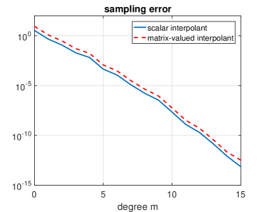
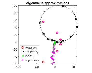
Figure 1: Solution of a nonlinear eigenvalue problem using the AAA algorithm combined with NLEIGS. Left: Accuracy of the AAA sampling procedure as the degree $m$ of the rational interpolant increases. Right: Exact eigenvalues and their approximations, together with the sampling points $z_{j}$ and the poles $\xi_{j}$ of the rational interpolant.

5 Conclusions

We have derived explicit formulas for converting between rational interpolants in barycentric, rational Krylov (RKFUN), and Newton form, and shown two examples where this conversion is useful within the RKToolbox. In future work we plan to extend the sampling procedure to nonsquare problems, e.g., for sampling solutions of vector-valued initial and boundary value problems, and we plan to derive probabilistic error bounds for the surrogate sampling approach.

Acknowledgements. The authors would like to thank the Engineering and Physical Sciences Research Council (EPRSC) and Sabisu for providing SE with a CASE PhD studentship. SG is grateful to Yuji Nakatsukasa, Olivier Sète, and Nick Trefethen for their hospitality during his sabbatical in 2016, and for many interesting discussions on the AAA algorithm and nonlinear eigenvalue problems which stimulated this work.

References

- [1] Bagby, T. On interpolation by rational functions. Duke Math. J. 36, 1 (1969), 95–104.
- [2] Berljafa, M. Rational Krylov Decompositions: Theory and Applications. PhD thesis, The University of Manchester, Manchester, UK, 2017. Available as MIMS EPrint 2017.6 at http://eprints.ma.man.ac.uk/2529/.
- [3] Berljafa, M., and Güttel, S. A Rational Krylov Toolbox for MATLAB. MIMS EPrint 2014.56, Manchester Institute for Mathematical Sciences, The University of Manchester, UK, 2014. Available for download at http://rktoolbox.org.
- [4] Berljafa, M., and Güttel, S. Generalized rational Krylov decompositions with an application to rational approximation. SIAM J. Matrix Anal. Appl. 36, 2 (2015), 894–916.
- [5] Berljafa, M., and Güttel, S. The RKFIT algorithm for nonlinear rational approximation. SIAM J. Sci. Comput. 39, 5 (2017), A2049–A2071.
- [6] Güttel, S., Beeumen, R. V., Meerbergen, K., and Michiels, W. NLEIGS: A class of fully rational Krylov methods for nonlinear eigenvalue problems. SIAM J. Sci. Comput. 36, 6 (2014), A2842–A2864.
- [7] Güttel, S., and Tisseur, F. The nonlinear eigenvalue problem. Acta Numer. 26 (2017), 1–94.
- [8] Klein, G. Applications of linear barycentric rational interpolation. PhD thesis, Université de Fribourg, 2012.
- [9] Lawrence, P. W., and Corless, R. M. Stability of rootfinding for barycentric Lagrange interpolants. Numer. Algorithms 65, 3 (2014), 447–464.
- [10] Mehrmann, V., and Voss, H. Nonlinear eigenvalue problems: A challenge for modern eigenvalue methods. GAMM-Mitt. 27 (2004), 121–152.
- [11] Nakatsukasa, Y., Sète, O., and Trefethen, L. N. The AAA algorithm for rational approximation. arXiv preprint arXiv:1612.00337 (2016).
- [12] Ruhe, A. Rational Krylov algorithms for nonsymmetric eigenvalue problems. II. Matrix pairs. Linear Algebra Appl. 198 (1994), 283–295.
- [13] Schneider, C., and Werner, W. Some new aspects of rational interpolation. Math. Comp. 47, 175 (1986), 285–299.
- [14] Van Beeumen, R., Meerbergen, K., and Michiels, W. Compact rational Krylov methods for nonlinear eigenvalue problems. SIAM J. Matrix Anal. Appl. 36, 2 (2015), 820–838.