Transport coefficients in neutron star cores in BHF approach. Comparison of different nucleon potentials

Abstract

Thermal conductivity and shear viscosity of npe$\mu$ matter in non-superfluid neutron star cores are considered in the framework of Brueckner-Hartree-Fock many-body theory. We extend our previous work (Shternin et al 2013 PRC 88 065803) by analysing different nucleon-nucleon potentials and different three-body forces. We find that the use of different potentials leads up to one order of magnitude variations in the values of the nucleon contribution to transport coefficients. The nucleon contribution dominates the thermal conductivity, but for all considered models the shear viscosity is dominated by leptons.

1 Introduction

Transport coefficients serve as an important part of the microphysical input required for modelling of various non-equilibrium processes in neutron stars (NSs). For instance, thermal conductivity is needed to study the NS cooling (especially at early stages) and thermal wave propagation from internal heating sources [1]. Viscosity coefficients regulate the damping and stability of the oscillation modes within the stars [2]. In these proceedings we consider the nucleon contribution to the thermal conductivity $\kappa$ and the shear viscosity $\eta$ in non-superfluid NS cores in equilibrium with respect to beta-processes with the simplest npe$\mu$ composition. Transport coefficients of a mixture are governed by the collisions between the species. In NS cores conditions, the lepton and nucleon sub-systems decouple and these sectors can be considered separately (e.g., [3]).

In [4], $\kappa$ and $\eta$ were calculated in the non-relativistic Brueckner-Hartree-Fock (BHF) approach for one particular nucleon-nucleon potential, Argonne v18 (Av18 in short) supplemented by the phenomenological Urbana IX (UIX in short) model for three-body forces. It is known, that purely two-body interactions in non-relativistic calculations can not correctly reproduce the empirical nuclear matter saturation point and the inclusion of three-body forces is necessary. Several models for the three-body forces are available on the market, and we investigate the model-dependence of the results obtained in [4]. In this respect, we employ the same microscopic potentials as in [5], where appropriate references and more detailed discussion can be found. Namely, in addition to the Av18+UIX model, we also use the CD-Bonn two-body potential with the corresponding adjustment of UIX three-body interaction. Both the Av18+UIX and CD-Bonn+UIX combinations reproduce the correct saturation point. In addition, we employ the three-body force obtained within the meson-nucleon theory, where the same meson-exchange parameters are used for two- and three- body interactions. As in [5], we use this model constructed for Argonne v18 potential and denote it as Av18+TBF.

2 Formalism

The contribution of each strongly degenerate species’ in the mixture can be written as (we omit the species index, for brevity)

$$\kappa=C_{\kappa}\frac{\pi^{2}k_{\rm B}^{2}Tn}{3m^{*}}\tau,\quad\eta=C_{\eta}\frac{p_{{\rm F}}^{2}n}{5m^{*}}\tau,$$ (1)

where $T$ is the temperature, $p_{\rm F}$ is the Fermi momentum, $n$ is the number density, $m^{*}$ is the effective mass on the Fermi surface, $k_{\rm B}$ is the Boltzmann constant, $\tau$ is the characteristic relaxation time and $C_{\kappa,\eta}$ are numerical constants. The latter values are found as a solution of the system of transport equations for the multicomponent Fermi-liquid. A method to obtain exact solution for these equations was developed in [6]. Below we adapt this formalism to the form convenient to perform the calculations for nuclear matter.

The necessary microscopic input is the values of $m^{*}$ and the quasiparticle scattering amplitude $\hat{T}$. We obtain $m^{*}$ and $\hat{T}$ within the BHF approximation, see [4] for details. Consider the scattering of two nucleon species $c$ and $i$, $c+i\to c^{\prime}+i^{\prime}$. We define ${\cal Q}_{ci}(P,q)=1/4(1+\delta_{ci})^{-1}\sum_{\rm spins}|\langle ci|\hat{T}|c^{\prime}i^{\prime}\rangle|^{2}$, where all particles are placed on the Fermi surface and the momentum and energy conservation delta-functions are taken out. This quantity depends on the total nucleon pair momentum $\bm{P}=\bm{p}_{c}+\bm{p}_{i}$ and the transferred momentum $\bm{q}=\bm{p}_{c}^{\prime}-\bm{p}_{c}$. In what follows we will need the angular averages ${\cal Q}_{ci}^{(kl)}=\langle{\cal Q}_{ci}P^{k}q^{l}\rangle$. The explicit definition for these averages which have the meaning of generalized transport cross-sections can be found in the appendix in [4]. When the nucleon interaction is expanded in partial waves, such representation is more convenient than the traditional use of the Abrikosov-Khalatnikov angles [4].

In transport theory, one expresses a non-equilibrium distribution function $F(\bm{p},\epsilon)$ by introducing a linear (in external perturbation) correction to the local equilibrium distribution function as

$$F(\bm{p},\epsilon)=f(\epsilon)+\tau\Psi(x)D(\bm{p})\frac{\partial f}{\partial\epsilon},$$ (2)

where $f(\epsilon)$ is the Fermi-Dirac distribution, $x=(\epsilon-\mu)/(k_{\rm B}T)$, $\mu$ is the chemical potential and $D(\bm{p})$ is the anisotropic part of the driving term. For example, $D(\bm{p})=\bm{v}\nabla T$ for thermal conductivity. The transport coefficients are given then by (1) with

$$C_{\kappa/\eta}=\xi\int\limits_{-\infty}^{+\infty}{\rm d}x\,\Xi(x)\Psi(x)f(x)(1-f(x)).$$ (3)

For the shear viscosity, $\Xi(x)=1$ and $\xi=1$, while for thermal conductivity, $\Xi(x)=x$ and $\xi=3/\pi^{2}$. The unknown functions $\Psi_{c}(x)$, where $c$ now enumerates particle species, are determined from integral equations, derived by the linearization of the system of transport equations [6] using (2). Defining the characteristic relaxation time as

$$\tau_{c}=\frac{4\pi^{2}\hbar^{7}p_{{\rm F}c}}{m_{c}^{*}(k_{\rm B}T)^{2}}{\cal N}_{c},\quad{\cal N}_{c}=\left(\sum_{i}m_{i}^{*^{2}}{\cal Q}_{ci}^{(00)}\right)^{-1},$$ (4)

one obtains the system of integral equations in a simple form

$$\Xi(x)f(-x)=\left(1+\frac{x^{2}}{\pi^{2}}\right)\Psi_{c}(x)f(-x)-\frac{2}{\pi^{2}}\int\limits_{-\infty}^{+\infty}{\rm d}\,x^{\prime}\,f(-x^{\prime})\frac{x-x^{\prime}}{1-{\rm e}^{x^{\prime}-x}}\sum_{i}\lambda_{ci}\Psi_{i}(x^{\prime}),$$ (5)

where all information about the quasiparticle scattering is encapsulated in the matrix $\lambda_{ci}$. For $\kappa$ and $\eta$ problems, the matrices $\lambda_{ci}$ are expressed through angular averages ${\cal Q}^{(kl)}_{ci}$ as

$$\lambda^{\kappa}_{cc} = {\cal N}_{c}\sum_{i}m_{i}^{*2}\left({\cal Q}_{ci}^{(00)}-\frac{1}{2p_{{\rm F}c}^{2}}{\cal Q}_{ci}^{(02)}\right)+\left.\lambda^{\kappa}_{ci}\right|_{i=c},$$ (6)

$$\lambda^{\kappa}_{ci} = \frac{\tau_{i}}{p_{{\rm F}c}^{2}\tau_{c}}{\cal N}_{c}\,m_{c}^{*}m^{*}_{i}\left({\cal Q}_{ci}^{(20)}-\left(p_{{\rm F}c}^{2}+p_{{\rm F}i}^{2}\right){\cal Q}_{ci}^{(00)}+\frac{1}{2}{\cal Q}_{ci}^{(02)}\right),$$ (7)

$$\lambda^{\eta}_{cc} = {\cal N}_{c}\sum_{i}m_{i}^{*2}\left({\cal Q}_{ci}^{(00)}-\frac{3}{2p_{{\rm F}c}^{2}}{\cal Q}_{ci}^{(02)}+\frac{3}{8p_{{\rm F}c}^{4}}{\cal Q}_{ci}^{(04)}\right)+\left.\lambda^{\eta}_{ci}\right|_{i=c},$$ (8)

$$\lambda^{\eta}_{ci} = \frac{3\tau_{i}}{4p_{{\rm F}c}^{4}\tau_{c}}{\cal N}_{c}\,m_{c}^{*}m^{*}_{i}\left({\cal Q}_{ci}^{(22)}-\left(p_{{\rm F}c}^{2}+p_{{\rm F}i}^{2}\right){\cal Q}_{ci}^{(02)}+\frac{1}{2}{\cal Q}_{ci}^{(04)}\right).$$ (9)

Provided the matrix $\lambda_{ci}$ is known, the solution of the system (5) can be found numerically by iteration method, as we do here. In [6] the general method is developed to express the solution in form of the rapidly converging series. The frequently used simplest variational solution corresponds to a first term in these series (namely, $\Psi(x)\propto\Xi(x)$). For carriers of one type, these variational solutions give $C_{\kappa}^{\rm Var}=1.25(3-\lambda^{\kappa}_{cc})^{-1}$ and $C_{\eta}^{\rm Var}=0.75(1-\lambda^{\eta}_{cc})^{-1}$ [6].

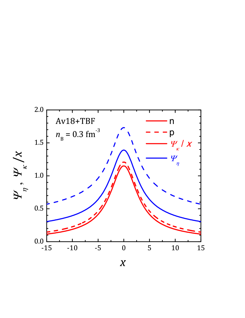
Figure 1: Functions $\Psi_{\eta}(x)$ and $\Psi_{\kappa}(x)/x$ for neutrons () and protons () from the exact solutions of the system (5) for the Av18+TBF microscopic model and $n_{\rm B}=0.3$ fm^-3. Thick red and thin blue lines correspond to thermal conductivity and shear viscosity problems, respectively.

3 Results and conclusions

As an example, consider the Av18+TBF model at the total baryon density $n_{\rm B}=0.3$ fm^-3 and $T=10^{8}$ K. The proton fraction of $\beta$-stable matter is $x_{\rm p}=0.1$, the effective masses (in units of nucleon mass) are $m_{\rm n}^{*}=0.81$ and $m_{\rm p}^{*}=0.67$ [5]. The neutron and proton effective relaxation times (4) are similar, $\tau_{\rm n}=1.2\times 10^{-16}$ s and $\tau_{\rm p}=0.79\times 10^{-16}$ s, but since $n_{\rm p}$ is much smaller than $n_{\rm n}$, the proton contribution to transport coefficients is small [see (1)]. The exact solutions of the system (5) are shown in figure 1 giving $C^{\rm n}_{\kappa}=0.67$ and $C^{\rm n}_{\eta}=1.21$ for the neutrons. The total value of the thermal conductivity is $\kappa=\kappa_{\rm n}+\kappa_{\rm p}=1.2\times 10^{23}$ erg cm^-1 s^-1 K^-1 and the total shear viscosity is $\eta=2.8\times 10^{18}$ g cm^-1 s^-1. It is instructive to note that the influence of $\Psi_{\rm p}(x)$ on the equation for $\Psi_{\rm n}(x)$ via the non-diagonal terms in (5) is negligible, since $\lambda_{\rm nn}^{\kappa}=0.07\lambda_{\rm np}^{\kappa}$ (???). However, the inverse is not true, $\lambda_{\rm pn}^{\kappa}=1.39\lambda_{\rm pp}^{\kappa}$ and the non-equilibrium neutron distribution strongly affects the proton one. Thus it seems a good starting approximation to consider only the neutron contribution to transport (but taking into account np collisions as well, see, e.g., [4]). In the present example, this gives $C_{\kappa}^{{\rm n},\ {\rm Var}}=0.55$ and $C_{\eta}^{{\rm n},\ {\rm Var}}=1.13$ where we additionally used the simplest variational solution. Comparing this approximation with the exact values, we get $\kappa/\kappa_{\rm n}^{{\rm Var}}=1.36$ and $\eta/\eta_{\rm n}^{{\rm Var}}=1.1$.

In figure 2 we present the final results of our calculations. We show the results for the Av18 potential on the two-body level and with addition of the UIX and TBF three-body forces. The CD-Bonn results on the two-body level give similar values as Av18 and are not shown, while the CD-Bonn+UIX results are shown with red dashed lines. For comparison, we show also the results obtained using free-space scattering probability and $m^{*}=1$ (dotted lines) as well as the lepton contribution (thin dashed lines). Notice, that the lepton contribution has non-Fermi-liquid temperature dependence ($\eta_{\rm e\mu}\propto T^{-5/3}$ and $\kappa_{\rm e\mu}={\rm const}(T)$) [7, 8]. One clearly sees the importance of in-medium effects. At a two-body level, both $\eta$ and $\kappa$ in-medium values are much higher than the results based on the free-space interaction. The inclusion of UIX three-body force acts in the opposite direction, partially (but not fully) due to the increase in particles’ effective masses [4, 5]. The effect of the meson-exchange three-body model TBF is much less pronounced, and the results stay approximately at the two-body level. In the future we plan to investigate the contribution of different partial waves to $\kappa$ and $\eta$ calculations in order to understand the difference in UIX and TBF effects.

The variations of $\kappa$ and $\eta$ found in our calculations are large. Fortunately, the shear viscosity is dominated by the lepton contribution, whose dependence on the equation of state is mainly through the particle fractions and effective masses and may be easily accounted for. For the thermal conductivity, the situation is reverse. However, the precise value of the thermal conductivity is usually not important since it is so large that the NS core is almost isothermal. In our study we did not consider the effects of the superfluidity that can be very important in NS cores. This is a good project for the future.

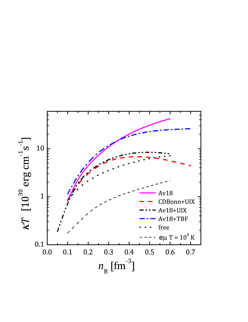
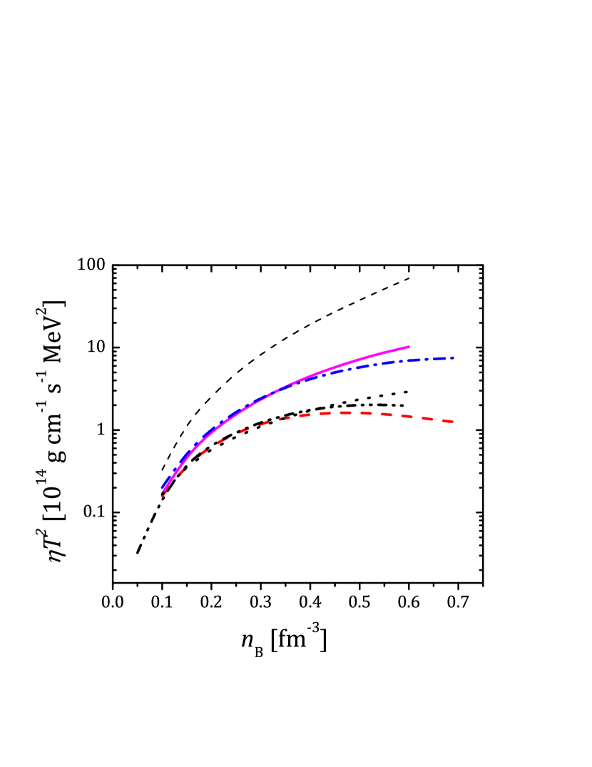
Figure 2: Temperature-independent combinations $\kappa T$ (left) and $\eta T^{2}$ (right) as functions of baryon number density for the models considered in the text. Thin dashed lines show lepton contribution for $T=10^{8}$ K and Av18+UIX EOS calculated according [7, 8].

The work of PSS was supported by the Russian Foundation for Basic Research, grant 16-32-00507 mol$\_$a and the “BASIS” Foundation.

References

References

- [1] Yakovlev D G, Kaminker A D, Gnedin O Y and Haensel P 2001 Phys. Rep. 354 1–155
- [2] Haskell B 2015 International Journal of Modern Physics E 24 1541007
- [3] Flowers E and Itoh N 1979 ApJ 230 847–58
- [4] Shternin P S, Baldo M and Haensel P 2013 Phys. Rev. C 88 065803
- [5] Baldo M, Burgio G F, Schulze H J and Taranto G 2014 Phys. Rev. C 89 048801
- [6] Anderson R H, Pethick C J and Quader K F 1987 Phys. Rev. B 35 1620–29
- [7] Shternin P S and Yakovlev D G 2007 Phys. Rev. D 75 103004
- [8] Shternin P S and Yakovlev D G 2008 Phys. Rev. D 78 063006