Structural Bifurcation Analysis in Chemical Reaction Networks

Abstract

In living cells, chemical reactions form a complex network. Complicated dynamics arising from such networks are the origins of biological functions. We propose a novel mathematical method to analyze bifurcation behaviors of a reaction system from the network structure alone. The whole network is decomposed into subnetworks based on “buffering structures”. For each subnetwork, the bifurcation condition is studied independently, and the parameters that can induce bifurcations and the chemicals that can exhibit bifurcations are determined. We demonstrate our theory using hypothetical and real networks.

I Introduction

In a living cell, a large set of chemical reactions are connected by sharing their products and substrates, and constructing a large network. Biological functions are believed to arise from dynamics of chemical concentrations based on the networks. It is also considered that regulations and adaptations of biological systems are realized by modulations of amount/activities of enzymes mediating reactions. In previous studies Mochizuki ; OM , we developed a mathematical method, by which the sensitivity responses of chemical reaction networks to perturbations of enzyme amount/activities are determined from network structures alone. Our method is based on an augmented matrix A (see Eq. (6)), in which the distribution of nonzero entries directly reflects network structures. One of the striking result is the law of localization OM . A substructure (subset of chemicals and reactions) in a reaction network satisfying a topological condition is called buffering structure (Fig. 1(1), (2)), and has the property that perturbations of reaction rate parameters inside a buffering structure influence only (steady-state) concentrations and fluxes inside this structure, and the outside remains unchanged under the perturbations.

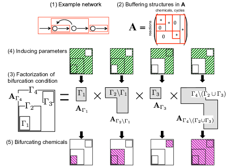
Figure 1: Summary of the structural bifurcation analysis. (1) Buffering structures (red boxes) in an example network. (2) Buffering structure corresponds to nonzero square blocks in A. (3) Bifurcations in the whole system are governed by a product of buffering structures with subtraction of their inner buffering structures. (4) For each subnetwork, parameters in shadowed area can induce bifurcations associated with the subnetwork. (5) For each subnetwork, chemicals in shadowed area exhibit bifurcations.

In this paper, we study another aspect governed by buffering structures: bifurcation behaviors of reaction systems. We prove that the determinant of the Jacobian matrix J of a reaction system is equivalent to that of the augmented matrix A for the corresponding network structure. Based on this equivalence, we study steady-state bifurcations of reaction systems from network structures. In this paper, our usage of “parameter” always means a parameter associated with a reaction rate.

From the structural bifurcation analysis based on the matrix A, we obtain the following general results on steady-state bifurcations in reaction networks.

(i) Factorization: A is factorized into submatrices based on the buffering structures (Fig. 1(3)). It implies that bifurcation behaviors in a complex network can be studied by decomposing it into smaller subnetworks, which are buffering structures with subtraction of their inner buffering structures. For each subnetwork, the condition of bifurcation occurrence is determined from the structure of the subnetwork.

(ii) Inducing parameters: For each subnetwork, bifurcation is induced by parameter changes which are neither in buffering structures inside the subnetwork nor those non-intersecting with the subnetwork (Fig. 1 (4)).

(iii) Bifurcating chemicals (and fluxes): When the condition of bifurcation associated with a subnetwork is satisfied, the bifurcation of steady-state concentrations (and fluxes) appears only inside the (minimal) buffering structure containing the subnetwork (Fig. 1 (5)).

These findings make it possible to study behaviors of a whole reaction system including multiple bifurcations based on inclusion relations of buffering structures. We apply our method to hypothetical and real networks, and demonstrate the practical usefulness to analyze behaviors of complex systems.

II Structural sensitivity analysis.—

We label chemicals by $m\,(m=1,\cdots,M)$ and reactions by $n\,(n=1,\cdots,N)$. A state of a spatially homogeneous chemical reaction system is specified by the concentrations $x_{m}(t)$, and obeys the differential equations Mochizuki ; F1 ; F2 :

$$\frac{dx_{m}}{dt}=\sum_{n=1}^{N}\nu_{mn}r_{n}({\mbox{\boldmath$x$}};k_{n}),\;m=1,\ldots,M.$$ (1)

Here, the $M\times N$ matrix $\nu$ is called the stoichiometric matrix, and its component $\nu_{mn}$ is defined as follows: Let the stoichiometry of the $n$-th reaction among chemical molecules $X_{m}$ be given by $\sum_{m=1}^{M}y^{n}_{m}X_{m}\rightarrow\sum_{m=1}^{M}\bar{y}^{n}_{m}X_{m}$ Then the $\nu_{mn}$ is given by $\nu_{mn}=\bar{y}^{n}_{m}-y^{n}_{m}.$ The reaction rate function (flux) $r_{n}$ depends on the concentration vector $x$ and also on rate parameters $k_{n}$.

To present the key idea, we start by assuming that the stoichiometric matrix $\nu$ does not have nonzero cokernel vectors, which in turn implies that ${\rm rank}(\nu)=M\leq N$ and the steady state concentration ${\mbox{\boldmath$x$}}^{*}$ and fluxes ${\mbox{\boldmath$r$}}^{*}$ are continuous functions of rate parameters $\{k_{n}\}_{n=1}^{N}$. The general case will be presented in the Supplemental Material (SM). For steady state ${\mbox{\boldmath$x$}}^{*}$, one can choose $\{\mu^{\alpha}\}_{\alpha=1}^{N-M}$ such that the corresponding steady state flux ${\mbox{\boldmath$r$}}^{*}$ is expressed, in terms of the basis $\{{\mbox{\boldmath$c$}}_{\alpha}\}_{\alpha=1}^{N-M}$ of the kernel space of $\nu$, as

$${\mbox{\boldmath$r$}}^{*}=\sum_{\alpha=1}^{K}\mu^{\alpha}{\mbox{\boldmath$c$}}_{\alpha},\quad K:=N-M={\rm\dim ker}\,\nu.$$ (2)

Now we review the structural sensitivity analysis Mochizuki and the law of localization OM . Under the perturbation $k_{\hat{n}}\to k_{\hat{n}}+\delta k_{\hat{n}}$ ($\hat{n}=1,\ldots,N$), the corresponding concentration changes $\delta_{\hat{n}}x_{m}$ and the flux changes $\delta_{\hat{n}}r_{n}$ at the steady state ${\mbox{\boldmath$x$}}^{*}$ are determined simultaneously by solving the following equation

$${\bf A}\left(\begin{array}[]{cccc}\delta_{1}{\mbox{\boldmath$x$}}&\ldots&\delta_{N}{\mbox{\boldmath$x$}}\\ \hline\cr\delta_{1}{\mbox{\boldmath$\mu$}}&\ldots&\delta_{N}{\mbox{\boldmath$\mu$}}\\ \end{array}\right)=-{\rm diag}\Big{(}\frac{\partial r_{1}}{\partial k_{1}}\delta k_{1},\ \ldots,\ \frac{\partial r_{N}}{\partial k_{N}}\delta k_{N}\Big{)},$$ (5)

where the horizontal line denotes the structure of block matrices, the derivatives are evaluated at the steady state ${\mbox{\boldmath$x$}}^{*}$, $\delta_{\hat{n}}{\mbox{\boldmath$\mu$}}=(\delta_{\hat{n}}\mu^{1},\ldots,\delta_{\hat{n}}\mu^{K})^{T}$ is the change of the coefficients $\mu^{\alpha}$ in (2) under the perturbation: $k_{\hat{n}}\to k_{\hat{n}}+\delta k_{\hat{n}}$, and the matrix ${\bf A}$ is given by

$${\bf A}=\Big{(}\frac{\partial{\mbox{\boldmath$r$}}}{\partial{\mbox{\boldmath$x$}}}\Big{|}_{{\mbox{\boldmath$x$}}={\mbox{\boldmath$x$}}^{*}}-{\mbox{\boldmath$c$}}_{1}\ldots-{\mbox{\boldmath$c$}}_{K}\Big{)}.$$ (6)

Here the entry $\partial r_{n}/\partial x_{m}$ in the left part of $\bf A$ is given by

$$\begin{cases}\frac{\partial{\color[rgb]{0,0,0}r}_{n}}{\partial x_{m}}\neq 0\ \ {\rm if}\ x_{m}\ {\rm influences\ reaction}\ n,\\ \frac{\partial{\color[rgb]{0,0,0}r}_{n}}{\partial x_{m}}=0\ \ {\rm otherwise.}\ \end{cases}$$ (7)

Note that whether each entry of A is zero or nonzero is determined structurally, that is, independently of detailed forms of rate functions and quantitative values of concentrations and parameters.

For a given network $\Gamma$, we consider a pair $\Gamma_{s}=({\mathfrak{m}},{\mathfrak{n}})$ of a chemical subset ${\mathfrak{m}}$ and a reaction subset ${\mathfrak{n}}$ satisfying the condition that ${\mathfrak{n}}$ includes all reactions influenced by chemicals in ${\mathfrak{m}}$ (in the sense of (7)). We call such a $\Gamma_{s}=({\mathfrak{m}},{\mathfrak{n}})$ as output-complete. For a subnetwork $\Gamma_{s}=(\mathfrak{m},\mathfrak{n})$, we define the index $\chi(\Gamma_{s})$ as

$$\chi(\Gamma_{s})=|\mathfrak{m}|-|\mathfrak{n}|+(\#cycle).$$ (8)

Here, $|\mathfrak{m}|$ and $|\mathfrak{n}|$ are the numbers of elements of the sets $\mathfrak{m}$ and $\mathfrak{n}$, respectively. The $\#cycle$ is the number of independent kernel vectors of the matrix $\nu$ whose supports are contained in $\mathfrak{n}$. In general, $\chi(\Gamma_{s})$ is non-positive (see OM ). Then a buffering structure is defined as an output-complete subnetwork $\Gamma_{s}$ with $\chi(\Gamma_{s})=0$.

Suppose that $\Gamma_{s}=({\mathfrak{m}},{\mathfrak{n}})$ is a buffering structure. By permutating the column and row indices, the matrix $\bf A$ can be written as follows: OM

$${\bf A}=\begin{array}[]{c }\ _{|{\mathfrak{n}}|}\big{\updownarrow}\\ \\ \end{array}\overset{\overset{|{\mathfrak{m}}|+(\#cycle)}{\ext@arrow 0099\arrowfill@\longleftarrow\relbar\longrightarrow{}{\hskip 30.00005pt}}\quad\quad\quad\quad}{\left(\begin{array}[]{ccc|c }&\underset{square}{\mbox{\smash{ ${\bf A}_{\Gamma_{s}}$}}}&&\ \ \ \ \mbox{\smash{\Large$*$}}\\ \hline\cr&\mbox{\smash{ $\bf 0$}}&&\ \ \ \mbox{\smash{ ${\bf A}_{\bar{\Gamma}_{s}}$}}\end{array}\right)},$$ (13)

where the rows (columns) of ${\bf A}_{\Gamma_{s}}$ are associated with the reactions (chemicals and cycles) in $\Gamma_{s}$. Similarly, those of ${\bf A}_{\bar{\Gamma}_{s}}$ are associated with the complement ${\bar{\Gamma}}_{s}:=\Gamma\backslash\Gamma_{s}$.

The law of localization OM is a direct consequence of the block structure (13) of the matrix A: Steady-state concentrations and fluxes outside of a buffering structure does not change under any rate parameter perturbations in $\mathfrak{n}$. In other words, all effects of perturbations of $k_{\hat{n}}$ in $\mathfrak{n}$ are indeed localized within $\Gamma_{s}$.

III Structural bifurcation analysis.—

We shortly sketch the conventional bifurcation analysis. Set $J:=\nu\frac{\partial{\mbox{\boldmath$r$}}}{\partial{\mbox{\boldmath$x$}}}|_{{\mbox{\boldmath$x$}}={\mbox{\boldmath$x$}}^{*}}$. Let the eigenvalues $\{\sigma_{m}\}_{m=1}^{M}$ of $J$ be ordered so that ${\rm Re}\,\sigma_{1}\geq{\rm Re}\,\sigma_{2}\ldots$. Then the state ${\mbox{\boldmath$x$}}^{*}$ is stable if all ${\rm Re}\,\sigma_{m}<0$, whereas, the state ${\mbox{\boldmath$x$}}^{*}$ is unstable if ${\rm Re}\,\sigma_{1}>0$. Moreover, a bifurcation occurs if ${\rm Re}\,\sigma_{1}$ changes its sign as some parameter $k_{\hat{n}}$ is varied through some critical value, say $\bar{k}_{\hat{n}}$. Since $\det J=\prod_{m=1}^{M}\sigma_{m}$, a bifurcation occurs if $\det J$ changes its sign as $k_{\hat{n}}$ is varied through $\bar{k}_{\hat{n}}$. Thus, the study of the onset of bifurcation is reduced to the search of the zeros of $\det J$.

Now, we explain structural bifurcation analysis. The following relation is the key to our method:

$$\det J\propto\det{\bf A},$$ (14)

where the proportionality constant depends only on the stoichiometric matrix $\nu$. See the SM for the proof. Then (57) implies that the study of the onset of bifurcation of system (1) can be reduced to the search of the zeros of ${\rm det}\,{\bf A}$. Further, the existence of the buffering structure $\Gamma_{s}$ of the network $\Gamma$ guarantees the following relation

$$\det J\propto\det{\bf A}_{\Gamma_{s}}\cdot\det{\bf A}_{\bar{\Gamma}_{s}}.$$ (15)

An extension of (15) to a nested sequence of buffering structures $\Gamma_{1}\subset\ldots\subset\Gamma_{L}$ gives the relation $\det J\propto\det{\bf A}_{\Gamma_{1}}\prod_{s=1}^{L-1}\det{\bf A}_{{\Gamma_{s+1}}\backslash{\Gamma_{s}}}$.

There are several implications of the factorization (15). First, from the equality $\det J=0$, we have either ${\rm det}\,{\bf A}_{\Gamma_{s}}=0$ or $\det{\bf A}_{\bar{\Gamma}_{s}}=0$. In other words, the possibility of bifurcation occurrences in the whole system can be studied by examining the possibility for each of the subnetworks from their structures.

Second, from the law of localization (see the SM for details), ${\rm det}\,{\bf A}_{\bar{\Gamma}_{s}}$ depends only on parameters outside $\Gamma_{s}$, whereas ${\rm det}\,{\bf A}_{\Gamma_{s}}$ depends on parameters in the whole network $\Gamma$. Thus, bifurcations associated with ${\rm det}\,{\bf A}_{\bar{\Gamma}_{s}}$ are triggered only by tuning parameters in $\bar{\Gamma}_{s}$, while bifurcations associated with ${\rm det}\,{\bf A}_{\Gamma_{s}}$ can be induced by both parameters in ${\Gamma_{s}}$ and those in ${\bar{\Gamma}_{s}}$ (see inducing parameters in Fig. 1 (4)). In particular, in the former case, critical values (values at bifurcation points) of parameters in ${\bar{\Gamma}_{s}}$ are independent of parameters in $\Gamma_{s}$.

Third, as shown in the SM, the null vector of the Jacobian $J$ at a bifurcation point with ${\rm det}\,{\bf A}_{\Gamma_{s}}=0$ has nonzero components only for chemicals in $\Gamma_{s}$. This implies that only chemicals in $\Gamma_{s}$ exhibit bifurcations at this bifurcation point. By contrast, for bifurcations associated with ${\rm det}\,{\bf A}_{\bar{\Gamma}_{s}}$, all chemicals in $\Gamma$ exhibit bifurcation behaviors (see bifurcating chemicals in Fig. 1 (5)). These three arguments are generalized into multiple buffering structures, as stated in the introductory part of this paper.

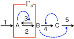
Figure 2: System consisting of five reactions, $\overset{k_{1}}{\rightarrow}{\rm A},$ $\ {\rm A}\underset{k_{2}}{\overset{k_{3}}{\leftrightharpoons}}{\rm B},\ {\rm B}\overset{k_{4}}{\rightarrow}{\rm C},\ {\rm C}\overset{k_{5}}{\rightarrow}$. The three blue dashed arcs indicate the regulations explained in the text. The red box indicates a buffering structure $\Gamma_{s}$.

IV Hypothetical network

We demonstrate the structural bifurcation analysis in the system shown in Fig. 2. The stoichiometry matrix $\nu$ and the kernel vectors are

$$\nu =\left(\begin{array}[]{ccccc}1&-1&1&0&0\\ 0&1&-1&-1&0\\ 0&0&0&1&-1\\ \end{array}\right),$$ (19)

$${\mbox{\boldmath$c$}}_{1} =(0,1,1,0,0)^{T},{\mbox{\boldmath$c$}}_{2}=(1,1,0,1,1)^{T}.$$ (20)

Every reaction rate depends on the substrate concentration. Reaction rates $r_{3},r_{5}$, and $r_{4}$ are also regulated by A, B, and C, respectively. Then, ${\Gamma_{s}}=(\{{\rm A}\},\{2,3\})$ is a buffering structure since $\chi(\Gamma_{s})=1-2+1=0$.

By permutating the row index as $\{2,3,1,4,5\}$ and the column index as $\{\text{A},{\mbox{\boldmath$c$}}_{1},\text{ B},\text{ C},{\mbox{\boldmath$c$}}_{2}\}$, the matrix ${\bf A}$ and the determinant are given by

$${\bf A}= \left(\begin{array}[]{c|c}{\bf A}_{\Gamma_{s}}&{\bf*}\\ \hline\cr{\bf 0}&{\bf A}_{\bar{\Gamma}_{s}}\end{array}\right)=\left(\begin{array}[]{ccccc}\cline{1-2}\cr\vrule\lx@intercol\hfil r_{2,\text{A}}\hfil\lx@intercol&\lx@intercol\hfil 1\hfil\lx@intercol\vrule\lx@intercol&0&0&1\\ \vrule\lx@intercol\hfil r_{3,\text{A}}\hfil\lx@intercol&\lx@intercol\hfil 1\hfil\lx@intercol\vrule\lx@intercol&r_{3,\text{B}}&0&0\\ \cline{1-5}\cr 0&0&\vrule\lx@intercol\hfil 0\hfil\lx@intercol&0&\lx@intercol\hfil 1\hfil\lx@intercol\vrule\lx@intercol\\ 0&0&\vrule\lx@intercol\hfil r_{4,\text{B}}\hfil\lx@intercol&r_{4,\text{C}}&\lx@intercol\hfil 1\hfil\lx@intercol\vrule\lx@intercol\\ 0&0&\vrule\lx@intercol\hfil r_{5,\text{B}}\hfil\lx@intercol&r_{5,\text{C}}&\lx@intercol\hfil 1\hfil\lx@intercol\vrule\lx@intercol\\ \cline{3-5}\cr\end{array}\right),$$ (28)

$${\rm det}\,{\bf A} =\underset{{\rm det}\,{\bf A}_{\Gamma_{s}}}{\underbrace{\left(r_{2,\text{A}}-r_{3,\text{A}}\right)}}\underset{{\rm det}\,{\bf A}_{\bar{\Gamma}_{s}}}{\underbrace{\left(r_{5,\text{B}}r_{4,\text{C}}-r_{4,\text{B}}r_{5,\text{C}}\right)}},$$ (29)

where nonzero $\frac{\partial r_{n}}{\partial x_{m}}|_{{\mbox{\boldmath$x$}}={\mbox{\boldmath$x$}^{*}}}$ is written by $r_{n,m}$, $m=$ A, B, C. Due to the expression of $\det{\bf A}$, we conclude that the regulations corresponding to $r_{3,{\rm A}}$ and $(r_{4,{\rm C}},r_{5,{\rm B}})$ are necessary for bifurcations associated with ${\rm det}\,{\bf A}_{\Gamma_{s}}=0$ and ${\rm det}\,{\bf A}_{\bar{\Gamma}_{s}}=0$, respectively. In this way, the possibility of bifurcation occurrences can be examined structurally for each subnetwork.

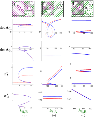
Figure 3: Steady-state values of $\det\,{\bf A}_{{\Gamma}_{s}}$ , $\det\,{\bf A}_{\bar{\Gamma}_{s}}$ , $x_{A}^{*}$, $x_{C}^{*}$ versus $k_{5,{\rm B}}$ in (a), $k_{3,\rm A}$ in (b), $k_{5,{\rm B}}$ in (c). Red and blue curves correspond to two choices of parameters in ${\Gamma_{s}}$ in (a) and (c), two choices of parameters in ${\bar{\Gamma}_{s}}$ in (b). In the top panel of each case, the dark-colored region indicates the subnetwork whose determinant changes its sign at the bifurcation point, and the green- and purple-shaded regions indicate the inducing parameters and bifurcating chemicals, respectively. See the SM for the specific parameter values used for the plots.

For numerical demonstration, we assume the following kinetics:

$${\mbox{\boldmath$r$}}= \biggl{(}k_{1},k_{2}x_{\text{A}},k_{3}x_{\text{B}}\left(1+\frac{k_{3,\text{A}}x_{\text{A}}^{2}}{x_{\text{A}}^{2}+5}\right),$$

$$k_{4}x_{\text{B}}\left(1+\frac{k_{4,\rm{C}}x_{\text{C}}^{2}}{x_{\text{C}}^{2}+5}\right),k_{5}x_{\text{C}}\left(1+\frac{k_{5,\rm{B}}x_{\text{B}}^{2}}{x_{\text{B}}^{2}+5}\right)\biggr{)}.$$ (30)

The parameters are classified into $\{k_{2},k_{3},k_{3,A}\}\in{\Gamma_{s}}$, and $\{k_{1},k_{4},k_{5},k_{4,{\rm C}},k_{5,{\rm B}}\}\in{\bar{\Gamma}_{s}}$.

First, we consider a bifurcation associated with ${\rm det}\,{\bf A}_{\bar{\Gamma}_{s}}$. The inducing parameters for the subnetwork ${\bar{\Gamma}_{s}}$ are the parameters in ${\bar{\Gamma}}_{s}$ (the green-shaded region in the top panel of Fig. 3a). As seen from the plots of ${\rm det}\,{\bf A}_{\Gamma_{s}}$ and ${\rm det}\,{\bf A}_{\bar{\Gamma}_{s}}$ in Fig. 3a, the parameter $k_{5,{\rm B}}$ in ${\bar{\Gamma}_{s}}$ actually induces sign changes of ${\rm det}\,{\bf A}_{\bar{\Gamma}_{s}}$ but not those of ${\rm det}\,{\bf A}_{\Gamma_{s}}$ (two saddle-node bifurcations). The bifurcating chemicals for ${\bar{\Gamma}_{s}}$ are all chemicals $\{\text{A, B, C}\}$ (see the purple-shaded region of the top panel). Fig. 3a actually shows that both chemicals A and C exhibit steady-state bifurcations. On the other hand, varying parameters in ${\Gamma_{s}}$ changes only concentrations in $\Gamma_{s}$, due to the law of localization. This is illustrated by the blue and red curves in Fig. 3a. We see that only the concentration of chemical A changes as parameters in ${\Gamma_{s}}$ are varied, while the critical value of the bifurcation parameter $k_{5,B}$ is independent of parameters in ${\Gamma_{s}}$.

Next, we consider the other bifurcation, which is associated with ${\rm det}\,{\bf A}_{\Gamma_{s}}$. The inducing parameters for the subnetwork ${\Gamma_{s}}$ consist of all parameters in ${\Gamma_{s}}$ and ${\bar{\Gamma}_{s}}$ (see the green-shaded region in the top panels of Fig. 3b). The plots of ${\rm det}\,{\bf A}_{\Gamma_{s}}$ in Fig. 3b show that the parameter $k_{3,{\rm A}}\in\Gamma_{s}$ indeed induces bifurcations associated with ${\rm det}\,{\bf A}_{\Gamma_{s}}$. The bifurcating chemicals for ${\Gamma_{s}}$ are the chemicals in ${\Gamma_{s}}$, i.e. $\{\text{A}\}$ (the purple-shaded region in the top panel). This can be confirmed from the plots for $x^{*}_{\rm A},x^{*}_{\rm C}$ in Fig. 3b, where only the steady-state of chemical A $\in{\Gamma_{s}}$ bifurcates at the bifurcation point, while chemical C $\in{\bar{\Gamma}_{s}}$ remains constant as $k_{3,{\rm A}}\in{\Gamma_{s}}$ is varied, due to the law of localization. The law of localization also implies that varying parameters in ${\bar{\Gamma}}_{s}$ can change concentrations of all chemicals. This is illustrated by the two curves in Fig. 3b, where two different values of parameters in ${{\bar{\Gamma}_{s}}}$ result in different concentration values for both of chemicals A and C. In addition, varying parameters in ${\bar{\Gamma}_{s}}$ also influences the critical value of the bifurcation parameter $k_{3,\rm A}$.

There is another choice of bifurcation parameter for the bifurcation associated with ${\rm det}\,{\bf A}_{\Gamma_{s}}$, as the inducing parameters for ${\Gamma_{s}}$ are not only parameters in ${\Gamma_{s}}$ but also those in ${\bar{\Gamma}_{s}}$ (see the green-shaded region in the top panel of Fig. 3c). The parameter $k_{5,\rm B}\in{\bar{\Gamma}_{s}}$, which was chosen as a bifurcation parameter in Fig. 3a, also induces the bifurcation associated with ${\rm det}\,{\bf A}_{\Gamma_{s}}$ (see the plots for ${\rm det}\,{\bf A}_{\Gamma_{s}}$ in Fig. 3c). This implies that the same parameter may induce bifurcations for different sets of chemicals depending on which factor of ${\rm det}\,{\bf A}_{\Gamma_{s}}$ and ${\rm det}\,{\bf A}_{{\bar{\Gamma}_{s}}}$ changes its sign at the critical points. As in the case of Fig. 3b, the bifurcating chemicals are in $\Gamma_{s}$ (see the purple-shaded region in the top panel of Fig. 3c). Thus we see that only chemical ${\rm A}\in\Gamma_{s}$ bifurcates at the critical point in Fig. 3c. In particular, $k_{5,\rm B}$ does not induce the bifurcations of chemicals in ${\bar{\Gamma}_{s}}$, unlike the case of Fig. 3a. On the other hand, because of the law of localization, parameters in ${\Gamma_{s}}$ influence only chemical ${\rm A}\in{\Gamma_{s}}$, as illustrated by the two curves in Fig. 3c, corresponding to two different values of parameters in ${{\Gamma_{s}}}$. By contrast to Fig. 3a, the critical value of the bifurcation parameter $k_{5,B}\in{{\bar{\Gamma}}_{s}}$ is influenced by parameters in ${\Gamma_{s}}$.

V E. coli network

Finally, as a real example, we study the network of the central carbon metabolism of E. coli OM shown in Fig. 4, consisting of 28 chemicals and 46 reactions. The network possesses 17 buffering structures in it. As shown in the SM, there is only one single subnetwork (colored in red in Fig. 4) that can satisfy the bifurcation condition. Reactions associated with the inducing parameters for the red subnetwork are colored in red and green. The bifurcating chemicals (and fluxes) are colored in red and blue. We confirmed this behavior numerically (see Fig. S4 in the SM).

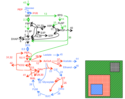
Figure 4: Central carbon metabolic network of E. coli. Dashed curve indicates a regulation from PEP to reaction 11 ($r_{11,{\rm PEP}}>0$). 　The right panel shows simplified inclusion relation of buffering structures.

Our method is applicable to any steady-state bifurcations of reaction systems even if systems have cokernel vectors. In the SM, we apply our theory to a phosphorylation system CC with cokernel vectors (i.e. conserved concentrations), and the First Schlögl Model schlogl , exhibiting transcritical bifurcations.

VI Conclusion and perspectives

In this paper we propose a mathematical method to study bifurcation behaviors of reaction systems from network structures alone. In our method, bifurcations of the whole complex system are studied by factorizing it into smaller substructures defined from buffering structures. For each substructure, the bifurcation condition is studied, and a set of parameters possibly inducing onset of bifurcation is determined.

Biological functions and their regulations are considered to arise from dynamics based on reaction networks and modulation of the enzymes. On the other hand, the complexity of networks has been a large obstacle to understand such systems. Our theory should be strongly effective to study dynamical behaviors of complex networks and promote systematic understandings of biological systems.

This work was supported partly by the CREST program (Grant No. JPMJCR13W6) of the Japan Science and Technology Agency (JST), by iTHES Project/iTHEMS Program RIKEN, by Grant-in-Aid for Scientific Research on Innovative Area, Logics of Plant Development (Grant No. 25113001), by NCTS and MOST of Taiwan. We express our sincere thanks to Gen Kurosawa, and Masashi Tachikawa for their helpful discussions and comments.

Supplemental Material 
Structural Bifurcation Analysis in Chemical Reaction Networks

Takashi Okada, Je-Chiang Tsai, and Atsushi Mochizuki

Appendix A Notation

• $\mathbb{X}=\{X_{1},\ldots,X_{M}\}$: the set of chemicals in the network. To ease the discussion, we also use the number index $m$ to identify the $m$-th chemical $X_{m}$. The reader can distinguish this difference from the context.

• $x_{m}$: the concentration of the $m$-th chemical, $m=1,\ldots,M$.

• $\mathbb{E}=\{E_{1},\ldots,E_{N}\}$: the set of reactions in the network. Again, in order to ease the notations, we also use the number index to identify the reaction.

• $r_{n}$: the reaction rate function associated with the $n$-th reaction, $n=1,\ldots,N$.

• $k_{n}$: the rate parameter associated with the reaction rate function $r_{n}$, $n=1,\ldots,N$. Note that the reaction rate function $r_{n}$ is a function of $x_{m}$, $m=1,\ldots,M$. Here we assume that the $n$-th reaction rate function $r_{n}$ has only one rate parameter $k_{n}$ involved. But the analysis performed here indicates that we do not need this assumption. We do this just for the ease of presentation. Thus $r_{n}=r_{n}({\mbox{\boldmath$x$}};k_{n})$ where ${\mbox{\boldmath$x$}}=(x_{1},\ldots,x_{M})^{T}$ and $T$ denotes the transpose operator of a matrix.

• ODE

  $$\frac{dx_{m}}{dt}=f_{m}(x_{1},\ldots,x_{M};k_{1},\ldots,k_{n}):=\sum_{n=1}^{N}\nu_{mn}r_{n}({\mbox{\boldmath$x$}};k_{n}),\;m=1,\ldots,M.$$ (1)

• $\{{\mbox{\boldmath$c$}}^{\alpha}\}_{\alpha=1}^{K}$ is the basis of the kernel space of the matrix $\nu=(\nu_{mn})_{M\times N}$. $K:={\rm dim\,ker}\,\nu$. The steady state value ${\mbox{\boldmath$r$}}^{*}$ of the reaction is given by a linear combination of them. We write the coefficient of ${\mbox{\boldmath$c$}}^{\alpha}$ by $\mu_{\alpha}$, i.e. ${\mbox{\boldmath$r$}}^{*}=\sum_{\alpha=1}^{K}\mu_{\alpha}{\mbox{\boldmath$c$}}^{\alpha}$.

• $\{{\mbox{\boldmath$d$}}_{\beta}\}_{\beta=1}^{K_{c}}$ is the basis of the cokernel space of the matrix $\nu$ (i.e., ${\mbox{\boldmath$d$}}_{\beta}^{T}\nu=0$ for each $\beta=1,\ldots,K_{c}$). $K_{c}:={\rm dim\,coker}\,\nu$. For each ${\mbox{\boldmath$d$}}_{\beta}$, using (1) the quantity $l_{\beta}\equiv{\mbox{\boldmath$d$}}_{\beta}\cdot{{\mbox{\boldmath$x$}}}$ is conserved with respect to time $t$.

Set

$${\mbox{\boldmath$f$}}=(f_{1},\ldots,f_{M})^{T},\;{\mbox{\boldmath$r$}}=(r_{1},\ldots,r_{N})^{T},\mbox{ and }\;{\mbox{\boldmath$k$}}=(k_{1},\ldots,k_{N})^{T}.$$

Then we can rewrite (1) as follows:

$$\frac{d{\mbox{\boldmath$x$}}}{dt}={\mbox{\boldmath$f$}}({\mbox{\boldmath$x$}};\mbox{\boldmath$k$}):=\nu{\mbox{\boldmath$r$}}.$$ (2)

Appendix B The equivalence between the Jacobian matrix and the matrix A

In this section, we prove the equivalence between the Jacobian and the matrix A. Systems with $K_{c}:={\rm dim\,coker}\,\nu=0$ are discussed in section B.1 (see (10)) and those with $K_{c}>0$ in section B.2 (see (57)).

B.1 The proof of the equivalence when $K_{c}=0$

To establish (10), we first note that the assumption $K_{c}=0$ implies that $N\geq M$ and $K=N-M$, where $K:={\rm dim\ ker}\ \nu$. Then employing the QR decomposition to the matrix $\nu^{T}$, we can factor the $\nu^{T}$ as the product of an $N\times N$ unitary matrix ${\bf Q}$ and an $N\times M$ upper triangular matrix $\tilde{{\bf S}}^{T}$ where $\tilde{{\bf S}}^{T}$ is the transpose of the matrix $\tilde{{\bf S}}$. As the bottom $K$ rows of an $N\times M$ upper triangular matrix consist entirely of zeroes, we thus have

$$\nu^{T}={\bf Q}\tilde{{\bf S}}^{T}=[{\bf Q}_{1}\;{\bf Q}_{2}]\left[\begin{array}[]{c}{\bf S}^{T}\\ {\bf 0}_{K\times M}\\ \end{array}\right]={\bf Q}_{1}{\bf S}^{T},$$ (5)

where ${\bf S}^{T}$ is an $M\times M$ upper triangular matrix, ${\bf 0}_{K\times M}$ is the $K\times M$ zero matrix, ${\bf Q}_{1}$ is a $N\times M$ matrix, ${\bf Q}_{2}$ is a $N\times K$ matrix, and both ${\bf Q}_{1}$ and ${\bf Q}_{2}$ have orthogonal columns. Further, the column space of ${\bf Q}_{1}$ is equal to the row space of $\nu$, whereas the column space of ${\bf Q}_{2}$ is equal to the null space of $\nu$, which follows from the fact that the row space of any nontrivial matrix is the orthogonal complement to its null space. To summarize, we have $\nu={\bf S}{\bf Q}_{1}^{T}.$ For simplicity, we let the basis $\{-{\bf c}_{\alpha}\}_{\alpha=1}^{K}$ consist of the columns of ${\bf Q}_{2}$.

Set ${\bf w}=[{\bf w}_{1}\;\;{\bf w}_{2}]^{T}:={\bf Q}^{T}\frac{\partial{\mbox{\boldmath$r$}}}{\partial{\mbox{\boldmath$x$}}},$ where ${\bf w}_{1}$ is a $M\times M$ matrix, and ${\bf w}_{2}$ is a $K\times M$ matrix. Recall that ${\bf Q}{\bf Q}^{T}=I_{N}$. Then we can rewrite the matrix $\frac{\partial{\mbox{\boldmath$r$}}}{\partial{\mbox{\boldmath$x$}}}$ of $r$ at the steady state ${\mbox{\boldmath$x$}}^{*}$ as follows:

$$\frac{\partial{\mbox{\boldmath$r$}}}{\partial{\mbox{\boldmath$x$}}}={\bf Q}({\bf Q}^{T}\frac{\partial{\mbox{\boldmath$r$}}}{\partial{\mbox{\boldmath$x$}}})\\ =\big{[}{\bf Q}_{1}\;{\bf Q}_{2}\big{]}\left[\begin{array}[]{c}{\bf w}_{1}\\ {\bf w}_{2}\\ \end{array}\right]={\bf Q}_{1}{\bf w}_{1}+{\bf Q}_{2}{\bf w}_{2}.$$ (6)

Together with (5) and the orthogonal property of ${\bf Q}$, we can deduce that

$$\begin{array}[]{ll}J=\nu\dfrac{\partial{\mbox{\boldmath$r$}}}{\partial{\mbox{\boldmath$x$}}}=({\bf S}{\bf Q}_{1}^{T})({\bf Q}_{1}{\bf w}_{1}+{\bf Q}_{2}{\bf w}_{2})={\bf S}{\bf w}_{1}.\end{array}$$ (7)

This in turn implies $\det(J)=\det({\bf S})\det({\bf w}_{1}).$ Recall that the rank (rank($\nu$)) of the matrix $\nu$ is $M$. Then we have ${\rm rank}({\bf S})={\rm rank}({\bf S}{\bf Q}_{1}^{T})={\rm rank}(\nu)=M$. Hence ${\bf S}$ is a square matrix of full rank, and so we can conclude that

$$\det({\bf w}_{1})=\big{(}\det({\bf S})\big{)}^{-1}\det(J).$$ (8)

On the other hand, in view of the orthogonal properties of ${\bf Q},{\bf Q}_{1}$, and ${\bf Q}_{2}$, the matrix A (defined in the main text) can be written as

$${\bf A}=[\frac{\partial{\mbox{\boldmath$r$}}}{\partial{\mbox{\boldmath$x$}}}\;{\bf Q}_{2}]=[{\bf Q}{\bf w}\;\;{\bf Q}_{2}]={\bf Q}[{\bf w}\;\;{\bf Q}^{T}{\bf Q}_{2}]={\bf Q}\Big{[}\begin{array}[]{l}{\bf w}_{1}\\ {\bf w}_{2}\\ \end{array}\begin{array}[]{l}{\bf 0}_{M\times K}\\ I_{K}\\ \end{array}\Big{]}.$$

Since ${\bf Q}$ is a square orthogonal matrix with $\det({\bf Q})=\pm 1$, we can thus deduce

$$\det({\bf w}_{1})=\pm\det({\bf A}).$$ (9)

Then from (8) and (9), we obtain the following result.

Theorem 1

$$\det({\bf A})=\pm\frac{\det(J)}{\det({\bf S})}.$$ (10)

B.2 The proof of the equivalence when $K_{c}>0$

B.2.1 The Jacobian matrix ${\tilde{J}}$ for $K_{c}>0$

To study the stability of (2) around a steady state, we need to compute the associated Jacobian matrix $J=D_{\mbox{\boldmath$x$}}{\mbox{\boldmath$f$}}=\nu\frac{\partial{\mbox{\boldmath$r$}}}{\partial{\mbox{\boldmath$x$}}}$. On the other hand, when $K_{c}>0$, there are only ${\tilde{M}}\equiv M-K_{c}$ independent variables in the set $\{x_{m}\}_{m=1}^{M}$. Thus we need to eliminate $K_{c}$ redundant variables from the set $\{x_{m}\}_{m=1}^{M}$ before computing the Jacobian matrix $J$.

Indeed, when $K_{c}>0$, without loss of generality, we may assume that the first $K_{c}$ rows of $\nu$ are linearly dependent. Then we can rewrite $\nu$ in the following form Klipp ,

$$\nu=\left(\begin{array}[]{c}{\tilde{\nu}}\\ L{\tilde{\nu}}\end{array}\right)=\left(\begin{array}[]{c}I_{{\tilde{M}}}\\ L\end{array}\right){\tilde{\nu}},$$ (15)

where ${\tilde{\nu}}$ is a ${\tilde{M}}\times N$ matrix, and $L$ (called a link matrix) is a $K_{c}\times{\tilde{M}}$ matrix. Here the matrix $I_{{\tilde{M}}}$ is the ${\tilde{M}}\times{\tilde{M}}$ identity matrix. In the remaining of this appendix, the terminology for the $n\times n$ identity matrix $I_{n}$ with $n\in\mathbb{N}$ is employed.

Decompose ${\mbox{\boldmath$x$}}\in\mathbb{R}^{M}$ as follows:

$${\mbox{\boldmath$x$}}=\left(\begin{array}[]{c}{\mbox{\boldmath$x$}}_{ind}\\ {\mbox{\boldmath$x$}}_{dep}\end{array}\right),$$

where ${\mbox{\boldmath$x$}}_{ind}\in{\mathbb{R}}^{{\tilde{M}}}$ and ${\mbox{\boldmath$x$}}_{dep}\in{\mathbb{R}}^{K_{c}}$. With these notations defined as above, we can rewrite the ODE system (1) (or (2)) in the following form,

$$\frac{d{\mbox{\boldmath$x$}}}{dt}=\frac{d}{dt}\left(\begin{array}[]{c}{\mbox{\boldmath$x$}}_{ind}\\ {\mbox{\boldmath$x$}}_{dep}\end{array}\right)=\left(\begin{array}[]{c}I_{\tilde{M}}\\ L\end{array}\right){\tilde{\nu}}{\color[rgb]{0,0,0}{\mbox{\boldmath$r$}}}.$$ (20)

Note $\frac{d}{dt}{\mbox{\boldmath$x$}}_{dep}=L{\tilde{\nu}}{\mbox{\boldmath$r$}}=L\frac{d}{dt}{\mbox{\boldmath$x$}}_{ind}$. Then an integration of this identity indicates that the ODE system (20) is equivalent to the following system:

$$\frac{d}{dt}{\mbox{\boldmath$x$}}_{ind} ={\tilde{\nu}}{\color[rgb]{0,0,0}{\mbox{\boldmath$r$}}},$$ (21)

$$-L{\mbox{\boldmath$x$}}_{ind}+{\mbox{\boldmath$x$}}_{dep} =constant.$$ (22)

Now we compute the Jacobian matrix ${\tilde{J}}$ associated with the ODE system (21). To proceed, let ${\mbox{\boldmath$x$}}^{*}=({\mbox{\boldmath$x$}}^{*}_{ind},{\mbox{\boldmath$x$}}^{*}_{dep})$ be a steady state of (20). Note that the reaction function $r$ depends not only on ${\mbox{\boldmath$x$}}_{ind}$, but also on ${\mbox{\boldmath$x$}}_{dep}$. Then the Jacobian matrix ${\tilde{J}}$ associated with the ODE system (21) around ${\mbox{\boldmath$x$}}^{*}_{ind}$ is given by

$$\begin{array}[]{ll}{\tilde{J}}={\tilde{\nu}}\dfrac{d{\mbox{\boldmath$r$}}}{d{\mbox{\boldmath$x$}_{ind}}}&:={\tilde{\nu}}\Big{(}\dfrac{\partial{\mbox{\boldmath$r$}}}{\partial{\mbox{\boldmath$x$}}_{ind}}+\dfrac{\partial{\mbox{\boldmath$r$}}}{\partial{\mbox{\boldmath$x$}}_{dep}}\cdot\dfrac{\partial{\mbox{\boldmath$x$}}_{dep}}{\partial{\mbox{\boldmath$x$}}_{ind}}\Big{)}\biggr{|}_{{\mbox{\boldmath$x$}}={\mbox{\boldmath$x$}}^{*}}\\[10.76385pt] &={\tilde{\nu}}\Big{(}\dfrac{\partial{\mbox{\boldmath$r$}}}{\partial{\mbox{\boldmath$x$}}_{ind}}+\dfrac{\partial{\mbox{\boldmath$r$}}}{\partial{\mbox{\boldmath$x$}}_{dep}}L\Big{)}\biggr{|}_{{\mbox{\boldmath$x$}}={\mbox{\boldmath$x$}}^{*}}\\[10.76385pt] &={\tilde{\nu}}\Big{(}\dfrac{\partial{\mbox{\boldmath$r$}}}{\partial{\mbox{\boldmath$x$}}_{ind}}+\dfrac{\partial{\mbox{\boldmath$r$}}}{\partial{\mbox{\boldmath$x$}}_{dep}}\Big{)}\biggr{|}_{{\mbox{\boldmath$x$}}={\mbox{\boldmath$x$}}^{*}}\cdot\left(\begin{array}[]{c}I_{{\tilde{M}}}\\ L\end{array}\right)\end{array}$$ (23)

Note that the size of ${\tilde{J}}$ is ${\tilde{M}}\times{\tilde{M}}$, that of $\frac{\partial{\mbox{\boldmath$r$}}}{\partial{\mbox{\boldmath$x$}}_{ind}}$ is $N\times{\tilde{M}}$, and that of $\frac{\partial{\mbox{\boldmath$r$}}}{\partial{\mbox{\boldmath$x$}}_{dep}}$ is $N\times K_{c}$.

B.2.2 QR decomposition of the stoichiometric matrix $\nu$ for $K_{c}>0$

Consider the QR decomposition of the ${\tilde{M}}\times N$ matrix ${\tilde{\nu}}$. First, since ${\tilde{\nu}}$ is of full rank, we have $N\geq{\tilde{M}}$. Then employing the QR decomposition to the matrix ${\tilde{\nu}}^{T}$, we can factor the ${\tilde{\nu}}^{T}$ as the product of an $N\times N$ unitary matrix ${\bf Q}$ and an $N\times{\tilde{M}}$ upper triangular matrix $\tilde{{\bf S}}^{T}$ where $\tilde{{\bf S}}^{T}$ is the transpose of the matrix ${\bf S}$. As the bottom $(N-{\tilde{M}})$ rows of an $N\times{\tilde{M}}$ upper triangular matrix consist entirely of zeroes, we thus have

$${\tilde{\nu}}^{T}={\bf Q}\tilde{{\bf S}}^{T}=[{\bf Q}_{1}\;{\bf Q}_{2}]\left[\begin{array}[]{c}{\bf S}^{T}\\ {\bf 0}_{(N-{\tilde{M}})\times{\tilde{M}}}\\ \end{array}\right]={\bf Q}_{1}{\bf S}^{T},$$

where ${\bf S}^{T}$ is an ${\tilde{M}}\times{\tilde{M}}$ upper triangular matrix, ${\bf 0}_{(N-{\tilde{M}})\times{\tilde{M}}}$ is the $(N-{\tilde{M}})\times{\tilde{M}}$ zero matrix, ${\bf Q}_{1}$ is a $N\times{\tilde{M}}$ matrix, ${\bf Q}_{2}$ is a $N\times(N-{\tilde{M}})$ matrix, and both ${\bf Q}_{1}$ and ${\bf Q}_{2}$ have orthogonal columns. Further, the column space of ${\bf Q}_{1}$ is equal to the row space of ${\tilde{\nu}}$, whereas the column space of ${\bf Q}_{2}$ is equal to the null space of ${\tilde{\nu}}$. The second statement follows from the fact that the row space of any nontrivial matrix is the orthogonal complement to its null space. To summarize, we have

$${\tilde{\nu}}={\bf S}{\bf Q}_{1}^{T}.$$ (24)

B.2.3 The matrix A for $K_{c}>0$ (review of OMpre )

We review the definition of the matrix A for $K_{c}>0$ OMpre and express it by using the bases of the kernel and cokernel spaces of $\nu$, introduced in the previous two sections. For a chemical reaction system with $K_{c}>0$, the steady state depends continuously on the reaction rate $k_{n}(n=1,\ldots,N)$ and also on the initial values of conserved concentrations, $l_{\beta}(\beta=1,\ldots,K_{c})$. Thus, we consider $N+K_{c}$ perturbations, in total. The sensitivity to the $N+K_{c}$ perturbations can be determined at once by solving the following equation,

$${\bf A}\left(\begin{array}[]{cccc}\delta_{1}{\mbox{\boldmath$x$}}&\ldots&\delta_{N+K_{c}}{\mbox{\boldmath$x$}}\\ \hline\cr\delta_{1}{\mbox{\boldmath$\mu$}}&\ldots&\delta_{N+K_{c}}{\mbox{\boldmath$\mu$}}\\ \end{array}\right)=-\left(\begin{array}[]{c| c}{\bf E}_{N}&{\bf 0}\\ \hline\cr{\bf 0}&{\bf E^{\prime}}_{K_{c}}\end{array}\right),$$ (29)

where ${\bf E}_{N}$ and ${\bf E^{\prime}}_{K_{c}}$ are $N\times N$ and $K_{c}\times K_{c}$ diagonal matrices, respectively, whose components are proportional to the perturbations; the $n$-th component of ${\bf E}_{N}$ is given by $\frac{\partial r_{n}}{\partial k_{n}}\delta k_{n}$, and the $\beta$-th component of ${\bf E}_{K_{c}}$ is given by $\delta l_{\beta}$. The matrix ${\bf A}$ is given by

$${\bf A}:=\begin{array}[]{c}\\ \ _{N}\Bigg{\updownarrow}\\ \\ \ _{K_{c}}\Bigg{\updownarrow}\\ \\ \end{array}\underset{\underset{M}{\ext@arrow 0099\arrowfill@\longleftarrow\relbar\longrightarrow{}{\hskip 40.00006pt}}\ \ \ \ \ \ \underset{K}{\ext@arrow 0099\arrowfill@\longleftarrow\relbar\longrightarrow{}{\hskip 50.00008pt}}}{\left(\begin{array}[]{cccc|c }&&&&\\ &\mbox{\smash{ $\dfrac{\partial{\mbox{\boldmath$r$}}}{\partial{\mbox{\boldmath$x$}}}$}}&&&{-{\mbox{\boldmath$c$}}^{\,1}\ {\ldots}\ -{\mbox{\boldmath$c$}}^{\,K}}\\ &&&&\\ \hline\cr&{-({\mbox{\boldmath$d$}}_{\,1})^{T}}&&&\\ &\vdots&&&\mbox{\smash{\ ${\bf 0}_{K_{c}\times K}$}}\\ &{-({\mbox{\boldmath$d$}}_{\,K_{c}})^{T}}&&&\end{array}\right)},$$ (41)

where ${\bf 0}_{K_{c}\times K}$ is a $K_{c}\times K$ zero matrix. With a direct computation, one can see that the row vectors of the following $K_{c}\times M$ matrix,

$$D:=(-L\;\;I_{K_{c}})$$ (42)

spans the cokernel space of $\nu$. Recall that $\{{\mbox{\boldmath$d$}}_{\beta}\}_{\beta=1}^{K_{c}}$ is the basis of the cokernel space of the matrix $\nu$. To facilitate the computation, we set

$$\left(\begin{array}[]{c}-({\mbox{\boldmath$d$}}_{\,1})^{T}\\ \vdots\\ -({\mbox{\boldmath$d$}}_{\,K_{c}})^{T}\end{array}\right)=D.$$

Also recall that $\{{\mbox{\boldmath$c$}}^{\alpha}\}_{\alpha=1}^{K}$ is the basis of the kernel $ker(\nu)$ of the matrix $\nu$, and that the column space of ${\bf Q}_{2}$ is the kernel $ker({\tilde{\nu}})$ of the matrix ${\tilde{\nu}}$. One can show that $ker(\nu)=ker({\tilde{\nu}})$. Motivated by this, we set

$$(-{\mbox{\boldmath$c$}}^{1},\ldots,-{\mbox{\boldmath$c$}}^{K})={\bf Q}_{2}.$$

Taken together, the matrix $\bf A$ takes the following form:

$${\bf A}=\begin{array}[]{c}\\ \ _{N}\Bigg{\updownarrow}\\ \ _{K_{c}}\bigg{\updownarrow}\\ \end{array}\underset{\underset{M}{\ext@arrow 0099\arrowfill@\longleftarrow\relbar\longrightarrow{}{\hskip 80.00012pt}}\ \ \ \ \ \ \underset{K}{\ext@arrow 0099\arrowfill@\longleftarrow\relbar\longrightarrow{}{\hskip 30.00005pt}}}{\left(\begin{array}[]{cccc|c }&&&&\\ &\mbox{\smash{ $\dfrac{\partial{\mbox{\boldmath$r$}}}{\partial{\mbox{\boldmath$x$}_{ind}}}$ \ $\dfrac{\partial{\mbox{\boldmath$r$}}}{\partial{\mbox{\boldmath$x$}_{dep}}}$}}&&&{{\bf Q}_{2}}\\ &&&&\\ \hline\cr&-L\hskip 34.14322ptI_{K_{c}}&&&\mbox{\smash{\ ${\bf 0}_{K_{c}\times K}$}}\\ \end{array}\right)}.$$ (50)

B.2.4 The relation between the Jacobian matrix ${\tilde{J}}$ and the matrix A for $K_{c}>0$

Set

$${\bf w}=\left[\begin{array}[]{c}{\bf w}_{1}\\ {\bf w}_{2}\\ \end{array}\right]:={\bf Q}^{T}\frac{d{\mbox{\boldmath$r$}}}{d{\mbox{\boldmath$x$}}_{ind}}\\ ={\bf Q}^{T}(\frac{\partial{\mbox{\boldmath$r$}}}{\partial{\mbox{\boldmath$x$}}_{ind}}+\frac{\partial{\mbox{\boldmath$r$}}}{\partial{\mbox{\boldmath$x$}}_{dep}}L),$$ (51)

where ${\bf w}_{1}$ is a ${\tilde{M}}\times{\tilde{M}}$ matrix, and ${\bf w}_{2}$ is a $(N-{\tilde{M}})\times{\tilde{M}}$ matrix. Recall that ${\bf Q}{\bf Q}^{T}=I_{N}$. Then we can rewrite the matrix $\frac{d{\mbox{\boldmath$r$}}}{d{\mbox{\boldmath$x$}}_{ind}}$ as follows:

$$\begin{array}[]{ll}\dfrac{d{\mbox{\boldmath$r$}}}{d{\mbox{\boldmath$x$}}_{ind}}&={\bf Q}({\bf Q}^{T}\dfrac{d{\mbox{\boldmath$r$}}}{d{\mbox{\boldmath$x$}}_{ind}}),\\[8.61108pt] &=\big{[}{\bf Q}_{1}\;{\bf Q}_{2}\big{]}\left[\begin{array}[]{c}{\bf w}_{1}\\ {\bf w}_{2}\\ \end{array}\right]={\bf Q}_{1}{\bf w}_{1}+{\bf Q}_{2}{\bf w}_{2}.\end{array}$$ (52)

Recall that ${\tilde{\nu}}={\bf S}{\bf Q}_{1}^{T}$. Together with the fact that ${\bf Q}_{1}^{T}{\bf Q}_{1}=I_{\tilde{M}}$ and ${\bf Q}_{1}^{T}{\bf Q}_{2}={\bf 0}_{{\tilde{M}}\times(N-{\tilde{M}})}$ where ${\bf 0}_{{\tilde{M}}\times(N-{\tilde{M}})}$ is the ${\tilde{M}}\times(N-{\tilde{M}})$ zero matrix, we can deduce that

$$\begin{array}[]{ll}{\tilde{J}}={\tilde{\nu}}\dfrac{d{\mbox{\boldmath$r$}}}{d{\mbox{\boldmath$x$}}_{ind}}&=({\bf S}{\bf Q}_{1}^{T})({\bf Q}{\bf w})\\ &=({\bf S}{\bf Q}_{1}^{T})({\bf Q}_{1}{\bf w}_{1}+{\bf Q}_{2}{\bf w}_{2}).\\ &={\bf S}{\bf w}_{1}.\end{array}$$ (53)

This in turn implies

$$\det({\tilde{J}})=\det({\bf S})\det({\bf w}_{1}).$$

Recall that the rank of the matrix ${\tilde{\nu}}$ is $rank({\tilde{\nu}})={\tilde{M}}$. Then we have $rank({\bf S})=rank({\bf S}{\bf Q}_{1}^{T})=rank({\tilde{\nu}})={\tilde{M}}$. Hence ${\bf S}$ is a square matrix of full rank. Thus we can conclude that

$$\det({\bf w}_{1})=\frac{\det({\tilde{J}})}{\det({\bf S})}.$$ (54)

On the other hand, using (51) we have

$${\bf A}=\left(\begin{array}[]{cccc|c }&&&&\\ &\mbox{\smash{ $\dfrac{\partial{\mbox{\boldmath$r$}}}{\partial{\mbox{\boldmath$x$}_{ind}}}$ \quad$\dfrac{\partial{\mbox{\boldmath$r$}}}{\partial{\mbox{\boldmath$x$}_{dep}}}$}}&&&{{\bf Q}_{2}}\\ &&&&\\ \hline\cr&-L\hskip 34.14322ptI_{K_{c}}&&&\mbox{\smash{\ ${\bf 0}_{K_{c}\times K}$}}\\ \end{array}\right)=\left(\begin{array}[]{cccc|c }&&&&\\ &\mbox{\smash{ ${\bf Q}{\bf w}-\dfrac{\partial{\mbox{\boldmath$r$}}}{\partial{\mbox{\boldmath$x$}_{dep}}}L$ \quad$\dfrac{\partial{\mbox{\boldmath$r$}}}{\partial{\mbox{\boldmath$x$}_{dep}}}$}}&&&{{\bf Q}_{2}}\\ &&&&\\ \hline\cr&-L\hskip 56.9055ptI_{K_{c}}&&&\mbox{\smash{\ ${\bf 0}_{K_{c}\times K}$}}\\ \end{array}\right).$$

To compute $\det({\bf A})$, consider the matrix

$${\bf B}=\left(\begin{array}[]{cccc|c }&&&&\\ &\mbox{\smash{ ${\bf Q}{\bf w}$ \quad${\bf Q}_{2}$}}&&&\dfrac{\partial{\mbox{\boldmath$r$}}}{\partial{\mbox{\boldmath$x$}_{ind}}}\\ &&&&\\ \hline\cr&{\bf 0}_{K_{c}\times{\tilde{M}}}\hskip 28.45274pt{\bf 0}_{K_{c}}&&&\mbox{\smash{\ $I_{K_{c}}$}}\\ \end{array}\right).$$

It is verified that $\det({\bf A})=(-1)^{K_{c}(K_{c}+1)/2}\det({\bf B})$. Thus it suffices to consider the matrix

$${\bf C}:=[{\bf Q}{\bf w}\;\;{\bf Q}_{2}].$$

In view of the fact that ${\bf Q}^{T}{\bf Q}=I_{N}$, ${\bf Q}_{1}^{T}{\bf Q}_{2}={\bf 0}_{{\tilde{M}}\times(N-{\tilde{M}})}$, and ${\bf Q}_{2}^{T}{\bf Q}_{2}=I_{N-{\tilde{M}}}$, we have

$${\bf Q}^{T}{\bf C}=[{\bf Q}^{T}{\bf Q}{\bf w}\;\;{\bf Q}^{T}{\bf Q}_{2}]=\Big{[}{\bf w}\begin{array}[]{l}{\bf 0}_{M\times(N-{\tilde{M}})}\\ I_{N-{\tilde{M}}}\\ \end{array}\Big{]}=\Big{[}\begin{array}[]{l}{\bf w}_{1}\\ {\bf w}_{2}\\ \end{array}\begin{array}[]{l}{\bf 0}_{M\times(N-{\tilde{M}})}\\ I_{N-{\tilde{M}}}\\ \end{array}\Big{]}.$$

This in turn implies

$${\bf C}={\bf Q}\Big{[}\begin{array}[]{l}{\bf w}_{1}\\ {\bf w}_{2}\\ \end{array}\begin{array}[]{l}{\bf 0}_{M\times(N-{\tilde{M}})}\\ I_{N-{\tilde{M}}}\\ \end{array}\Big{]}.$$ (55)

Since ${\bf Q}$ is a square orthogonal matrix with $\det({\bf Q})=\pm 1$, we can thus deduce

$$\det({\bf w}_{1})=\pm\det({\bf A}).$$ (56)

Then from (54) and (56), we can conclude the following theorem.

Theorem 2

The following equality holds.

$$\det({\bf A})=\pm\frac{\det({\tilde{J}})}{\det({\bf S})}.$$ (57)

Appendix C Structural Factorization of det A

Here, we explain the factorization of A in detail, after reviewing buffering structures and the law of localization. Systems with $K_{c}=0$ are discussed in section C.1, and those with $K_{c}>0$ in section C.2.

C.1 Structural Factorization when $K_{c}=0$

C.1.1 Buffering structure and the law of localization when $K_{c}=0$ (review of OM )

We construct a subnetwork $\Gamma_{s}=(\mathfrak{m},\mathfrak{n})$, a pair of chemicals and reactions, as follows:

1. Choose a subset $\mathfrak{m}\subseteq\mathbb{X}$ of chemicals.

2. Choose a subset $\mathfrak{n}\subseteq\mathbb{E}$ of reactions such that $\mathfrak{n}$ includes all reactions whose reaction rate functions $r_{n}(\mbox{\boldmath$x$})$ depend on at least one member in $\mathfrak{m}$. Namely, we can construct $\mathfrak{n}$ by collecting all reactions $n$ that are regulated by $\mathfrak{m}$ plus any other reactions.

Below, we consider only subnetworks constructed in this way and call them subnetworks. To proceed, we introduce the definition that a vector ${\bf v}\in\mathbb{R}^{N}$ has support contained in $\mathfrak{n}$. Indeed, for the reaction subset ${\mathfrak{n}}$, we can associate the vector space $V({\mathfrak{n}})$:

$$V({\mathfrak{n}}):=\,{\rm span}\,\bigl{\{}{\bf v}|\,{\bf v}\in{\rm ker}\,\nu,P^{\mathfrak{n}}{\bf v}={\bf v}\bigr{\}}.$$

Here, $P^{\mathfrak{n}}$ is an $N\times N$ projection matrix onto the space associated with ${\mathfrak{n}}$ defined by

$$P^{\mathfrak{n}}_{n,n^{\prime}}=\delta_{n,n^{\prime}}\ {\rm if}\ n,n^{\prime}\in{\mathfrak{n}}.\ {\rm Otherwise}\ P^{\mathfrak{n}}_{n,n^{\prime}}=0.$$

Then we say that a vector ${\bf v}\in\mathbb{R}^{N}$ has support contained in $\mathfrak{n}$ if ${\bf v}\in V({\mathfrak{n}})$.

For a subnetwork $\Gamma_{s}=(\mathfrak{m},\mathfrak{n})$, we define the index $\chi(\Gamma_{s})$ by the relation

$$\chi(\Gamma_{s})=|\mathfrak{m}|-|\mathfrak{n}|+(\#cycle).$$ (58)

Here, $|\mathfrak{m}|$ and $|\mathfrak{n}|$ are the number of elements in the sets $\mathfrak{m}$ and $\mathfrak{n}$, respectively. The $\#cycle$ is the number of independent kernel vectors of the matrix $\nu$ whose supports are contained in $\mathfrak{n}$. In general, $\chi(\Gamma_{s})$ is non-positive (see OM ).

Then a buffering structure is defined as a subnetwork $\Gamma_{s}$ with $\chi(\Gamma_{s})=0$.

It was proved in OM that, for a buffering structure $\Gamma_{s}=(\mathfrak{m},\mathfrak{n})$, the steady state values of chemical concentrations and reaction rates outside $\Gamma_{s}$ are independent of the reaction rate parameters $k_{n}$ of reactions in $\mathfrak{n}$. Specifically, let ${\mbox{\boldmath$x$}}^{*}=(x_{1}^{*},\ldots,x_{M}^{*})$ be the steady state of (1). Note that ${\mbox{\boldmath$x$}}^{*}$ depends on the parameter vector ${\mbox{\boldmath$k$}}=(k_{1},\ldots,k_{N})^{T}$. Set

$${\mbox{\boldmath$r$}}^{*}=(r_{1}^{*},\ldots,r_{N}^{*}):=(r_{1}({\mbox{\boldmath$x$}}^{*};k_{1}),\ldots,r_{N}({\mbox{\boldmath$x$}}^{*};k_{N})).$$

Then, for any $n^{\prime}\in\mathfrak{n}$, and any $m\in\mathfrak{m}^{c}$ and $n\in\mathfrak{n}^{c}$, one has

$$\frac{\partial x_{m}^{*}}{\partial k_{n^{\prime}}}=0,\;\;\frac{\partial r_{n}^{*}}{\partial k_{n^{\prime}}}=0,$$ (59)

where $\mathfrak{m}^{c}=\mathbb{X}\setminus\mathfrak{m}$ and $\mathfrak{n}^{c}=\mathbb{E}\setminus\mathfrak{n}$ are the complementary set of $\mathfrak{m}$ and $\mathfrak{n}$, respectively. For ease of notation, we set

$$\bar{\Gamma}_{s}:=(\mathfrak{m}^{c},\mathfrak{n}^{c}).$$

We remark that a whole network $\Gamma$ always satisfies the condition of the law of localization because $\chi(\Gamma)=M-N+K=K_{c}=0$.

C.1.2 Factorization of the matrix A when $K_{c}=0$

Suppose that $\Gamma_{s}$ is a buffering structure. Then, by permuting the columns and rows of the matrix A, the resulting matrix (still denoted by $\bf A$ for simplicity) can be written in the following form OM :

$${\bf A}=\begin{pmatrix}{\bf A}_{\Gamma_{s}}&{\bf A}_{\Gamma_{s},\bar{\Gamma}_{s}}\\ {\bf 0}_{|\mathfrak{n}^{c}|\times|\mathfrak{n}|}&{\bf A}_{\bar{\Gamma}_{s}}\end{pmatrix}.$$ (60)

The entries of ${\color[rgb]{0,0,0}{\bf A}_{\Gamma_{s}}}$ consist of components of the constant vectors ${\bf v}\in V(\mathfrak{n})$, and the term $\frac{\partial r_{n}}{\partial x_{m}}\big{|}_{{\mbox{\boldmath$x$}}={\mbox{\boldmath$x$}}^{*}}$ with $(m,n)\in\Gamma_{s}$ which corresponds to self-regulations inside $\Gamma_{s}$ (regulations from chemicals in $\Gamma_{s}$ to reaction rate functions in $\Gamma_{s}$). Similar characteristics for the entries of ${\bf A}_{\bar{\Gamma}_{s}}$ can be observed, which corresponds to self-regulations inside the complementary part $\bar{\Gamma}_{s}$. The non-constant entries of the upper-right matrix ${\bf A}_{\Gamma_{s},\bar{\Gamma}_{s}}$ correspond to regulations from $\bar{\Gamma}_{s}$ to $\Gamma_{s}$. Finally, the lower-left block in (60) is the zero matrix because (i) the kernel vectors in ${\Gamma_{s}}$ do not have support on reactions in $\mathfrak{n}^{c}$ and (ii) $\partial r_{n}/\partial x_{m}=0$ for $n\in\mathfrak{n}^{c}$, $m\in\mathfrak{m}$ follows from the condition that ${\Gamma_{s}}$ is output-complete (see also OM ).

Therefore, we have the following results.

Theorem 3

The following hold for a buffering structure $\Gamma_{s}$ in a network $\Gamma$.

1. The determinant of the matrix $\bf A$ can be factorized as follows:

   $$\det{\bf A}=\det{\bf A}_{\Gamma_{s}}\times\det{\bf A}_{\bar{\Gamma}_{s}}.$$ (61)

   Note that ${\bf A}_{\Gamma_{s},\bar{\Gamma}_{s}}$ does not contribute to $\det{\bf A}$.

2. $$\frac{\partial{\bf A}_{\bar{\Gamma}_{s}}}{\partial k_{n}}=0\ \ {\rm for}\ n\in\mathfrak{n}.$$ (62)

   Thus the complementary part ${\bf A}_{\bar{\Gamma}_{s}}$ is independent of the rate parameters $k_{n}$ with $n\in\mathfrak{n}$.

The assertion (ii) can be proved as follows: The entries of ${\bf A}_{\bar{\Gamma}_{s}}$ consist of the term $\frac{\partial r_{n^{\prime}}}{\partial x_{m^{\prime}}}\big{|}_{{\mbox{\boldmath$x$}}={\mbox{\boldmath$x$}}^{*}}$ with $(m^{\prime},n^{\prime})\in(\mathfrak{m}^{c},\mathfrak{n}^{c})$ and the components of the kernel vectors of the matrix $\nu$, which is obviously independent of $k_{n}$ for each $n=1,\ldots,N$. From the construction of the subnetwork $\Gamma_{s}$, $r_{n^{\prime}}$ are functions of variables $x_{m^{\prime}}$ with $m^{\prime}\in\mathfrak{m}^{c}$ , and so the derivatives $\frac{\partial r_{n^{\prime}}}{\partial x_{m^{\prime}}}\big{|}_{{\mbox{\boldmath$x$}}={\mbox{\boldmath$x$}}^{*}}$ can be written in terms of $x_{m^{\prime}}^{*}$ with $m^{\prime}\in\mathfrak{m}^{c}$. Then, these derivatives $\frac{\partial r_{n^{\prime}}}{\partial x_{m^{\prime}}}\big{|}_{{\mbox{\boldmath$x$}}={\mbox{\boldmath$x$}}^{*}}$ are independent of $k_{n}$ for $n\in\mathfrak{n}$ due to (59).

An important remark is that the above theorem can be applied not only to a single buffering structure but also for nested buffering structures. For example, a buffering structure within another larger buffering structure is studied similarly, by regarding $\Gamma$ as a larger buffering structure and $\Gamma_{s}$ as a smaller buffering structure in it.

In summary, for a buffering structure $\Gamma_{s}$ inside a network $\Gamma$, we have proved

$$\det{\bf A}_{\Gamma}=\det{\bf A}_{\Gamma_{s}}\times\underset{\underset{k_{\Gamma_{s}}}{{\rm independent\ of\ }}}{\underbrace{\det{\bf A}_{\bar{\Gamma}_{s}}}},$$ (63)

where $k_{\Gamma_{s}}$ denotes the set of parameters of reactions inside $\Gamma_{s}$.

C.1.3 Factorization for multiple buffering structures when $K_{c}=0$

We generalize the above factorization formula (63) into multiple buffering structures.

First, we consider a network $\Gamma$ containing $L$ non-intersecting buffering structures $\Gamma_{1},\ldots,\Gamma_{L}$. We write the complement of the buffering structures as $\bar{\Gamma}_{1,\ldots,L}:=\Gamma\backslash(\Gamma_{1}\cup\ldots\cup\Gamma_{L})$;

$$\Gamma=\Gamma_{1}\cup\ldots\cup\Gamma_{L}\cup{\bar{\Gamma}}_{1,\ldots,L}.$$ (64)

In this case, the matrix A can be written in the following form;

$${\bf A}=\left(\begin{array}[]{ccccc}\pagecolor[gray]{.8}{\bf A}_{\Gamma_{1}}&{\mbox{\boldmath$0$}}&\cdots&{\mbox{\boldmath$0$}}&{\bf A}_{\Gamma_{1},\bar{\Gamma}_{1,\ldots,L}}\\ {\mbox{\boldmath$0$}}&\pagecolor[gray]{.8}{\bf A}_{\Gamma_{2}}&\cdots&{\mbox{\boldmath$0$}}&{\bf A}_{\Gamma_{2},\bar{\Gamma}_{1,\ldots,L}}\\ \vdots&\vdots&\ddots&\vdots&\vdots\\ {\mbox{\boldmath$0$}}&{\mbox{\boldmath$0$}}&\cdots&\pagecolor[gray]{.8}{\bf A}_{\Gamma_{L}}&{\bf A}_{\Gamma_{L},\bar{\Gamma}_{1,\ldots,L}}\\ {\mbox{\boldmath$0$}}&{\mbox{\boldmath$0$}}&\cdots&{\mbox{\boldmath$0$}}&{\bf A}_{\bar{\Gamma}_{1,\ldots,L}}\end{array}\right),$$ (70)

where each shaded block ${\bf A}_{\Gamma_{s}}$ ($s=1,\ldots,L$) is an square matrix associated with ${\Gamma_{s}}$, defined as

$${\bf A}_{\Gamma_{s}}=\left(\begin{array}[]{c|ccc}({\frac{{\mbox{\boldmath$\partial$}{\mbox{\boldmath$r$}}}}{{\mbox{\boldmath$\partial$}}{\mbox{\boldmath$x$}}}})_{\Gamma_{s}}&{\mbox{\boldmath$c$}^{s}}_{1}&\ldots&{\mbox{\boldmath$c$}^{s}}_{K_{s}}\end{array}\right).$$ (72)

Here, the left block, $({\frac{{\mbox{\boldmath$\partial$}{\mbox{\boldmath$r$}}}}{{\mbox{\boldmath$\partial$}}{\mbox{\boldmath$x$}}}})_{\Gamma_{s}}$, consists of $\frac{\partial r_{n}}{\partial x_{m}}$ with $(m,n)\in\Gamma_{s}$, and the right block corresponds to the independent kernel vectors of $\nu$ whose support are on reactions in $\Gamma_{s}$ ($K_{s}$ is the number of the kernel vectors).

Then, we can prove that

$$\det{\bf A}=\biggl{(}\prod_{s=1}^{L}\underset{\underset{k_{\Gamma_{s}}{\rm\ and\ }k_{\bar{\Gamma}_{1,\ldots,L}}}{{\rm dependent\ on\ }}}{\underbrace{\det{\bf A}_{\Gamma_{s}}}}\biggr{)}\times\underset{\underset{k_{\bar{\Gamma}_{1,\ldots,L}}}{{\rm dependent\ on\ }}}{\underbrace{\det{\bf A}_{\bar{\Gamma}_{1,\ldots,L}}}},$$ (73)

where $k_{\Gamma^{\prime}}$ denotes the set of parameters associated with reactions inside a subnetwork $\Gamma^{\prime}$. The parameter dependence is determined by using (63) for every buffering structure $\Gamma_{s}$ ($s=1,\ldots,L$). For example, (63) for the buffering structure $\Gamma_{1}$ implies that the determinant factors except for ${\rm det}\,{\bf A}_{\Gamma_{1}}$ is independent of $k_{\Gamma_{1}}$ and so on.

We can also factorize a nested sequence of buffering structures. Consider a network $\Gamma$ consisting of a nested sequence of $L$ buffering structures $\Gamma_{1}\subset\ldots\subset\Gamma_{L}:=\Gamma$. In this case, the matrix A can be written as

$${\bf A}=\left(\begin{array}[]{ccccc}\pagecolor[gray]{.50}{\bf A}_{\Gamma_{1}}&\pagecolor[gray]{.7}{\mbox{\boldmath$*$}}&\pagecolor[gray]{.85 }{\mbox{\boldmath$*$}}&\pagecolor[gray]{.95 }\cdots&{\mbox{\boldmath$*$}}\\ \pagecolor[gray]{.7}{\mbox{\boldmath$0$}}&\pagecolor[gray]{.7}{\bf A}_{\Gamma_{2}\backslash\Gamma_{1}}&\pagecolor[gray]{.85 }\hfil&\pagecolor[gray]{.95}\cdots&{\mbox{\boldmath$*$}}\\ \pagecolor[gray]{.85 }{\mbox{\boldmath$0$}}&\pagecolor[gray]{.85 }{\mbox{\boldmath$0$}}&\pagecolor[gray]{.85 }{\bf A}_{\Gamma_{3}\backslash\Gamma_{2}}&\pagecolor[gray]{.95 }\hfil&\vdots\\ \pagecolor[gray]{.95}\vdots&\pagecolor[gray]{.95}\vdots&\pagecolor[gray]{.95}\hfil&\pagecolor[gray]{.95}\ddots&{\mbox{\boldmath$*$}}\\ {\mbox{\boldmath$0$}}&{\mbox{\boldmath$0$}}&\cdots&{\mbox{\boldmath$0$}}&{\bf A}_{\Gamma_{L}\backslash\Gamma_{L-1}}\end{array}\right),$$ (79)

where $*$’s indicate nonzero blocks and the gradation of shade indicates the nested sequence of buffering structures, $\Gamma_{1},\ldots,\Gamma_{L}$. By using (63) iteratively, we can prove

$$\det{\bf A}=\underset{\underset{k_{\Gamma_{L}}}{{\rm dependent\ on\ }}}{\underbrace{\det{\bf A}_{\Gamma_{1}}}}\prod_{s=1}^{L-1}\underset{\underset{k_{{\Gamma_{s+1}\backslash{\Gamma_{s}}}}}{{\rm dependent\ on\ }}}{\underbrace{\det{\bf A}_{{\Gamma_{s+1}}\backslash{\Gamma_{s}}}}}.$$ (80)

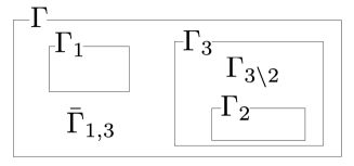
Figure S1: Example network $\Gamma$. Rectangular boxes, $\Gamma_{1},\,\Gamma_{2},\,\Gamma_{3}$, indicate buffering structures. The law of localization indicates that $k_{\Gamma_{1}}$ influences (steady-state values of chemicals and fluxes in) $\Gamma_{1}$, $k_{\Gamma_{3}}$ influences $\Gamma_{3}$, $k_{\Gamma_{3\backslash 2}}$ influences $\Gamma_{2}$, and $k_{\bar{\Gamma}_{1,3}}$ influences the whole network $\Gamma$.

By using (73) and (80), we can factorize the determinant of A for multiple buffering structures and determine the parameter dependence of each factor. We illustrate the procedure of factorization in an example network (see Fig. S1): Suppose that a whole network $\Gamma$ contains two non-intersecting buffering structures $\Gamma_{1}$ and $\Gamma_{3}$, and $\Gamma_{3}$ further contains a smaller buffering structure $\Gamma_{2}$ inside it;

$$\Gamma =\Gamma_{1}\cup\Gamma_{3}\cup\bar{\Gamma}_{1,3}$$

$$=\Gamma_{1}\cup(\Gamma_{2}\cup\Gamma_{3\backslash 2})\cup\bar{\Gamma}_{1,3}.$$ (81)

Here, $\bar{\Gamma}_{1,3}:=\Gamma\backslash(\Gamma_{1}\cup\Gamma_{3})$ and $\Gamma_{3\backslash 2}{\color[rgb]{0,0,0}:=}\Gamma_{3}\backslash\Gamma_{2}$. In this case, the matrix A can be written as

$${\bf A}=\left(\begin{array}[]{ccc}\pagecolor[gray]{.8}{\bf A}_{\Gamma_{1}}&{\mbox{\boldmath$0$}}&{\mbox{\boldmath$*$}}\\ {\mbox{\boldmath$0$}}&\pagecolor[gray]{.7}{\bf A}_{\Gamma_{3}}&{\mbox{\boldmath$*$}}\\ {\mbox{\boldmath$0$}}&{\mbox{\boldmath$0$}}&{\bf A}_{\bar{\Gamma}_{1,3}}\\ \end{array}\right)=\left(\begin{array}[]{cccc}\pagecolor[gray]{.8}{\bf A}_{\Gamma_{1}}&{\mbox{\boldmath$0$}}&{\mbox{\boldmath$0$}}&{\mbox{\boldmath$*$}}\\ {\mbox{\boldmath$0$}}&\pagecolor[gray]{.7}{\bf A}_{\Gamma_{2}}&\pagecolor[gray]{.7}{\mbox{\boldmath$*$}}&{\mbox{\boldmath$*$}}\\ {\mbox{\boldmath$0$}}&\pagecolor[gray]{.7}{\mbox{\boldmath$0$}}&\pagecolor[gray]{.9}{\bf A}_{\Gamma_{3\backslash 2}}&{\mbox{\boldmath$*$}}\\ {\mbox{\boldmath$0$}}&{\mbox{\boldmath$0$}}&{\mbox{\boldmath$0$}}&{\bf A}_{\bar{\Gamma}_{1,3}}\\ \end{array}\right),$$ (89)

and the determinant of A is factorized as

$${\rm det}\,{\bf A} =\underset{\underset{k_{\Gamma_{1}}{\rm\ and\ }k_{\bar{\Gamma}_{1,3}}}{{\rm depends\ on\ }}}{\underbrace{\det{\bf A}_{\Gamma_{1}}}}\times\underset{\underset{k_{\Gamma_{3}}{\rm\ and\ }k_{\bar{\Gamma}_{1,3}}}{{\rm depends\ on\ }}}{\underbrace{\det{\bf A}_{\Gamma_{3}}}}\times\underset{\underset{k_{\bar{\Gamma}_{1,3}}}{{\rm depends\ on\ }}}{\underbrace{{\rm det}\,{\bf A}_{\bar{\Gamma}_{1,3}}}}$$

$$=\underset{\underset{k_{\Gamma_{1}}{\rm\ and\ }k_{\bar{\Gamma}_{1,3}}}{{\rm depends\ on\ }}}{\underbrace{\det{\bf A}_{\Gamma_{1}}}}\times(\underset{\underset{k_{\Gamma_{2}},k_{\Gamma_{3\backslash 2}},{\rm\ and\ }k_{\bar{\Gamma}_{1,3}}}{{\rm depends\ on\ }}}{\underbrace{\det{\bf A}_{\Gamma_{2}}}}\times\underset{\underset{k_{\Gamma_{3\backslash 2}}{\rm\ and\ }k_{\bar{\Gamma}_{1,3}}}{{\rm depends\ on\ }}}{\underbrace{\det{\bf A}_{\Gamma_{3\backslash 2}}}})\times\underset{\underset{k_{\bar{\Gamma}_{1,3}}}{{\rm depends\ on\ }}}{\underbrace{{\rm det}\,{\bf A}_{\bar{\Gamma}_{1,3}}}}.$$ (90)

In the first line, we have used (73) with $L=2$ for the whole network $\Gamma$. In the second line, we have used (80) with $L=2$, namely (63), for the buffering structure $\Gamma_{3}$, where the factor ${\rm det}\,{\bf A}_{\Gamma_{3}}$ is factorized further and its dependence on $k_{\Gamma_{3}}$ is determined more finely.

C.2 Structural Factorization when $K_{c}>0$

C.2.1 Buffering structure and the law of localization when $K_{c}>0$ (review of OMpre )

The law of localization also holds when $K_{c}>0$ if we modify the definition of the index $\chi$ appropriately. Note that the construction of a subnetwork is the same as in the case $K_{c}=0$.

For a subnetwork $\Gamma_{s}=(\mathfrak{m},\mathfrak{n})$, we define $\chi$ as

$$\chi(\Gamma_{s})=|\mathfrak{m}|-|\mathfrak{n}|+(\#{\rm cycle})-(\#{\rm conserved\ concentration}).$$ (91)

Here, $(\#{\rm conserved\ concentration})$ counts conserved quantities in $\Gamma_{s}$, and is, more precisely, defined as the dimension of the vector space

$$V(\mathfrak{m}):={\rm span}\,\bigl{\{}P^{\mathfrak{m}}{\bf u}|{\bf u}\in\mathbb{R}^{M},\,{\bf u}^{T}\nu={\bf 0}\bigr{\}},$$ (92)

where $P^{\mathfrak{m}}$ is an $M\times M$ projection matrix for chemicals in $\mathfrak{m}$;

$$P^{\mathfrak{m}}_{m,m^{\prime}}=\delta_{m,m^{\prime}}{\ \rm if\ }m,m^{\prime}\in\mathfrak{m},\ {\rm otherwise}\ P^{\mathfrak{m}}_{m,m^{\prime}}=0.$$ (93)

Then, we again call a subnetwork $\Gamma_{s}$ a buffering structure when it satisfies $\chi(\Gamma_{s})=0$, where $\chi$ is defined by (91).

Recall that, when $K_{c}>0$, steady states generally depend on reaction rate parameters $k_{n}$ and the initial concentrations $l_{\beta}$. In OMpre , it was proved that, for a buffing structure $\Gamma_{s}$, the values of the steady state concentrations and fluxes outside of $\Gamma_{s}$ are independent of the reaction rate parameters and conserved quantities (initial conditions) associated with $\Gamma_{s}$. This is the generalized version of the law of localization into the case of $K_{c}>0$.

C.2.2 Factorization of the matrix $A$ when $K_{c}>0$

As discussed in OMpre , when $K_{c}>0$, by taking appropriate bases for the kernel and cokernel spaces of $\nu$ and permutating indices of the matrix, the matrix ${\bf A}$ can be again expressed as

$${\bf A}=\begin{pmatrix}{\bf A}_{\Gamma_{s}}&{\bf A}_{\Gamma_{s},\bar{\Gamma}_{s}}\\ {\bf 0}_{|\mathfrak{m}^{c}|\times|\mathfrak{n}^{c}|}&{\bf A}_{\bar{\Gamma}_{s}}\end{pmatrix},$$ (94)

where ${\bf A}_{\Gamma_{s}}$ is a square matrix, whose column(resp. row) indices correspond to chemicals and cycles (resp. reactions and conserved concentrations) associated with $\Gamma_{s}$.

Then, we obtain the following results.

Theorem 4

The following hold for a buffing structure $\Gamma_{s}$.

1. The determinant of the matrix $\bf A$ can be factorized as follows:

   $$\det{\bf A}=\det{\bf A}_{\Gamma_{s}}\times\det{\bf A}_{\bar{\Gamma}_{s}}.$$ (95)

   Thus ${\bf A}_{\Gamma_{s},\bar{\Gamma}_{s}}$ does not contribute to $\det{\bf A}$.

2. $$\frac{\partial{\bf A}_{\bar{\Gamma}_{s}}}{\partial k_{n}}=0,\ \frac{\partial{\bf A}_{\bar{\Gamma}_{s}}}{\partial l_{\beta}}=0\$$ (96)

   for reaction rate parameters $k_{n}$ and conserved concentrations $l_{\beta}$ associated with $\Gamma_{s}$.

(ii) can be proved in the same way as in (62): ${\bf A}_{\bar{\Gamma}_{s}}$ is a function of chemical concentrations in $\bar{\Gamma}_{s}$, whose steady-state values are independent of reaction rate parameters and conserved concentrations associated with $\Gamma_{s}$, due to the law of localization.

C.2.3 Factorization for multiple buffering structures when $K_{c}>0$

The factorization for multiple buffering structures is performed in the same way as in the case with $K_{c}=0$, except that, in the case of $K_{c}>0$, determinant factors in ${\rm det}\,{\bf A}$ depend not only on $k_{n}$ but also on that of $l_{\beta}$. From the law of localization, we can determine how parameters $k_{n}$ and conserved concentrations $l_{\beta}$ influences determinant factors, $\det{\bf A}_{\Gamma_{s}}$ and $\det{\bf A}_{\bar{\Gamma}_{s}}$, in (95) structurally.

Appendix D Null vectors of the matrix ${\bf A}$ and the Jacobian matrix, and bifurcating chemicals

Suppose that a chemical reaction system $\Gamma$ exhibits steady-state bifurcations. At a bifurcation point, there exist null vectors for the matrix A and the Jacobian matrix, since ${\rm det}\,{\bf A}={\rm det}\,J=0$. In the presence of a buffering structure $\Gamma_{s}$, the bifurcation is associated with either ${\rm det}\,{\bf A}_{\Gamma_{s}}=0$ or ${\rm det}\,{\bf A}_{\bar{\Gamma}_{s}}=0$.

In this section, we show that, for a bifurcation associated with ${\rm det}\,{\bf A}_{\Gamma_{s}}=0$, the null vector $v$ of the Jacobian matrix satisfies

$$v_{m}=0\ {\rm\ for}\ {\rm chemical\ }m\in{\bar{\Gamma}}_{s}.$$ (97)

Namely, $v$ has support inside chemicals in $\Gamma_{s}$. This implies that, for a bifurcation associated with ${\rm det}\,{\bf A}_{\Gamma_{s}}=0$, only chemicals inside $\Gamma_{s}$ undergo a bifurcating behavior.

D.1 Null vectors of the matrix A and the Jacobian matrix when $K_{c}=0$

The strategy for showing (97) is to use the null vectors of ${\rm A}_{\Gamma_{s}}$ to construct the associated null vector $v$ of the Jacobian matrix $J$.

We consider a chemical reaction system of $M$ chemicals and $N$ reactions where the cokernel space of $\nu$ consists only of the zero vector. Suppose that ${\rm det}\,{\bf A}_{\Gamma_{s}}=0$ whose associated buffering structure $\Gamma_{s}=(\mathfrak{m},\mathfrak{n})$ contains $|\mathfrak{m}|$ chemicals, $|\mathfrak{n}|$ reactions, and $K_{s}=|\mathfrak{n}|-|\mathfrak{m}|$ kernel vectors, $\{{\bf c}^{1},\ldots,{\bf c}^{K_{s}}\}$, of $\nu$. By construction, each ${\bf c}^{\alpha}\in\mathbb{R}^{N}$ ($\alpha=1,\ldots,K_{s}$) has support on reactions inside $\Gamma_{s}$, and thus has the following form,

$${\bf c}^{\alpha}=\left(\begin{array}[]{c}{\bf c}^{\prime\alpha}\\ \hline\cr{\bf 0}\end{array}\right),$$ (100)

where the upper $|\mathfrak{n}|$ components (resp. lower $N-|\mathfrak{n}|$ components) are associated with reactions in ${\Gamma_{s}}$ (resp. ${\bar{\Gamma}_{s}}$). By using ${\bf c}^{\prime\alpha}$, ${\bf A}_{\Gamma_{s}}$ in (60) can be written as

$${\bf A}_{\Gamma_{s}}=\left(\begin{array}[]{c|cc}(\dfrac{\partial{\mbox{\boldmath$r$}}}{\partial{\mbox{\boldmath$x$}}})_{{\Gamma_{s}}}&-{\bf c}^{\prime 1}\ldots&-{\bf c}^{\prime K_{s}}\end{array}\right),$$ (102)

where $(\dfrac{\partial{\mbox{\boldmath$r$}}}{\partial{\mbox{\boldmath$x$}}})_{{\Gamma_{s}}}$ is an $|\mathfrak{n}|\times|\mathfrak{m}|$ matrix whose $(n,m)$ component is given by $\frac{\partial r_{n}}{\partial x_{m}}$ with $n\in\mathfrak{n}$ and $m\in\mathfrak{m}$.

Since ${\rm det}\,{\bf A}_{\Gamma_{s}}=0$, there exist a null vector $\mbox{\boldmath$u$}_{s}\in\mathbb{R}^{|\mathfrak{m}|+K_{s}}$ such that

$${\bf A}_{\Gamma_{s}}{\mbox{\boldmath$u$}_{s}}=0.$$ (103)

If we write $\mbox{\boldmath$u$}_{s}=(\eta_{1},\ldots,\eta_{|\mathfrak{m}|},\zeta_{1},\ldots,\zeta_{K_{s}})$ and substitute ${\bf A}_{\Gamma_{s}}$ in (102) into Eq. (103), we obtain

$$\sum_{{\color[rgb]{0,0,0}m\in\mathfrak{m}}}\frac{\partial r_{n}}{\partial x_{m}}\eta_{m}-\sum_{\alpha=1}^{K_{s}}({\mbox{\boldmath$c$}^{\prime}}^{\alpha})_{n}\zeta_{\alpha}=0$$ (104)

for any reaction $n\in\mathfrak{n}$. Note that all indices in (104) are associated with $\Gamma_{s}$.

In order to relate (104) with the Jacobian matrix $J$ of the whole system $\Gamma$, we rewrite (104) using indices of the whole system. First, by using (100) and $\frac{\partial r_{n}}{\partial x_{m}}=0$ for $m\in\mathfrak{m},n\in\mathfrak{n}^{c}$, corresponding to the fact that chemical concentrations in a buffering structure does not appear in the arguments of rate functions of reactions outside the buffering structure, we can rewrite (104) as

$$\sum_{{\color[rgb]{0,0,0}m\in\mathfrak{m}}}\frac{\partial r_{n}}{\partial x_{m}}\eta_{m}-\sum_{\alpha=1}^{K_{s}}({\mbox{\boldmath$c$}}^{\alpha})_{n}\zeta_{\alpha}=0,$$ (105)

where $n$ is any reaction in the whole system $\Gamma=(\mathbb{X},\mathbb{E})$. Note that ${\mbox{\boldmath$c$}}^{\prime}$ has been replaced by $c$. Furthermore, by introducing an $M$-dimensional vector $v$ as ${\mbox{\boldmath$v$}}=({\mbox{\boldmath$\eta$}},\underset{M-|\mathfrak{m}|}{\underbrace{0,\ldots,0}})$, (105) can be rewritten as

$$\sum_{{\color[rgb]{0,0,0}m\in\mathbb{X}}}\frac{\partial r_{n}}{\partial x_{m}}\eta_{m}-\sum_{\alpha=1}^{K_{s}}({\mbox{\boldmath$c$}}^{\alpha})_{n}\zeta_{\alpha}=0,$$ (106)

where the summation of $m$ is taken over all chemicals in $\Gamma$. Finally, by multiplying (106) with the stoichiometry matrix $\nu$ and using the fact that ${\mbox{\boldmath$c$}}^{\alpha}$ is a kernel vector of $\nu$, we obtain

$$\sum_{{\color[rgb]{0,0,0}n\in\mathbb{E}}}\nu_{m^{\prime},n}\sum_{{\color[rgb]{0,0,0}m\in\mathbb{X}}}\frac{\partial r_{n}}{\partial x_{m}}v_{m}=0,$$ (107)

or, equivalently,

$$\sum_{{\color[rgb]{0,0,0}m\in\mathbb{X}}}J_{m^{\prime},m}v_{m}=0.$$ (108)

Thus, we have proved that ${\rm det}\,{\bf A}_{\Gamma_{s}}=0$ is associated with the null vector $v$ of the Jacobian matrix $J$, whose support is inside chemicals in $\Gamma_{s}$. Thus, (97) is proved.

A similar argument cannot be applied into a bifurcation associated with ${\rm det}\,{\bf A}_{\bar{\Gamma}_{s}}=0$. This difference comes from the nonsymmetric structure of the matrix A in (60); while columns associated with chemicals and kernels in ${\Gamma_{s}}$ do not have support on reactions in ${\bar{\Gamma}_{s}}$ (see zero entries in the lower-left block in (60)), those associated with ${\bar{\Gamma}_{s}}$ generally have support on both reactions in ${\bar{\Gamma}_{s}}$ and those in ${\Gamma_{s}}$ (see nonzero entries in the upper-right block in (60)). This implies that, while null vectors of $J$ associated with ${\rm det}\,{\bf A}_{{\Gamma_{s}}}=0$ do not have support on chemicals in ${\bar{\Gamma}_{s}}$, those associated with ${\rm det}\,{\bf A}_{{\bar{\Gamma}_{s}}}=0$ generally have support on both chemicals in ${\bar{\Gamma}_{s}}$ and those in ${\Gamma_{s}}$.

D.2 Null vectors of the matrix A and the Jacobian matrix when $K_{c}>0$

A similar result can also be proved when $K_{c}>0$. Let $\Gamma$ be a network system of $M$ chemicals and $N$ reactions whose corresponding stoichiometry matrix $\nu$ has $K$ kernel vectors and $K_{c}>0$ cokernel vectors (conserved concentrations).

Suppose that the subnetwork ${\Gamma_{s}}=(\mathfrak{m},\mathfrak{n})$ is a buffering structure. We separate the set of all chemicals $\mathbb{X}$ into two groups, $\mathbb{X}_{dep}$ and $\mathbb{X}_{ind}$, as in section B.2. Note that $K_{c}=|\mathbb{X}_{dep}|$ since each of cokernel vectors of $\nu$ corresponds to a chemical in $\mathbb{X}_{dep}$. Accordingly, we also separate the set of chemicals $\mathfrak{m}$ in ${\Gamma_{s}}$ into two groups, $\mathfrak{m}_{dep}:=\mathfrak{m}\cup\mathbb{X}_{dep}$ and $\mathfrak{m}_{ind}:=\mathfrak{m}\cup\mathbb{X}_{ind}$. Then, this buffering structure consists of $|\mathfrak{m}|=|\mathfrak{m}_{dep}|+|\mathfrak{m}_{ind}|$ chemicals, $|\mathfrak{n}|$ reactions, $K_{s}$ kernel vectors of $\nu$, and $|\mathfrak{m}_{dep}|$ conserved concentrations, satisfying $|\mathfrak{m}|-|\mathfrak{n}|+K_{s}-|\mathfrak{m}_{dep}|=0$.

The matrix ${\bf A}_{\Gamma_{s}}$ in (94) has the following form,

$${\bf A}_{\Gamma_{s}}=\left(\begin{array}[]{cc|c}(\dfrac{\partial{\mbox{\boldmath$r$}}}{\partial{\mbox{\boldmath$x$}}_{ind}})_{{\Gamma_{s}}}&(\dfrac{\partial{\mbox{\boldmath$r$}}}{\partial{\mbox{\boldmath$x$}}_{dep}})_{{\Gamma_{s}}}&-{\bf c}^{\prime 1}\ldots-{\bf c}^{\prime K_{s}}\\ \hline\cr-L_{\Gamma_{s}}&{\bf 1}_{K^{s}_{c}}&{\bf 0}_{K^{s}_{c}\times K_{s}}\end{array}\right).$$ (111)

Here, the column indices are associated with $\mathfrak{m}_{ind}$, $\mathfrak{m}_{dep}$, and kernel vectors of $\nu$ in $\Gamma_{s}$, from left to right, and the row indices are associated with $\mathfrak{n}$ and cokernel vectors associated with ${\Gamma_{s}}$. The left two blocks of ${\bf A}_{\Gamma_{s}}$ are obtained by taking columns and rows associated with $\Gamma_{s}$ from the left two block of the matrix A in (50): $(\dfrac{\partial{\mbox{\boldmath$r$}}}{\partial{\mbox{\boldmath$x$}}_{ind}})_{{\Gamma_{s}}}$ is an $N_{s}\times|\mathfrak{m}_{ind}|$ matrix, $(\dfrac{\partial{\mbox{\boldmath$r$}}}{\partial{\mbox{\boldmath$x$}}_{dep}})_{{\Gamma_{s}}}$ is an $N_{s}\times|\mathfrak{m}_{dep}|$ matrix. $L_{\Gamma_{s}}$ is an $|\mathfrak{m}_{dep}|\times|\mathfrak{m}_{ind}|$ matrix, which is the submatrix of the matrix $L$ in (50), obtained by taking the rows associated with $\mathfrak{m}_{dep}$ and columns associated with $\mathfrak{m}_{ind}$.

Suppose that ${\rm det}\,{\bf A}_{\Gamma_{s}}=0$. We denote the null vector $\mbox{\boldmath$u$}_{s}\in\mathbb{R}^{|\mathfrak{m}|+K_{s}}$ of ${\bf A}_{\Gamma_{s}}$ as

$${\mbox{\boldmath$u$}}_{s}=(\eta_{1},\ldots,\eta_{|\mathfrak{m}_{ind}|},\tilde{\eta}_{1},\ldots,\tilde{\eta}_{|\mathfrak{m}_{dep}|},\zeta_{1},\ldots,\zeta_{K_{s}})^{T}.$$ (112)

The equation ${\bf A}_{\Gamma_{s}}{\mbox{\boldmath$u$}}_{s}=0$ leads to the following two equations;

$$\sum_{m\in\mathfrak{m}_{ind}}\frac{\partial r_{n}}{\partial x_{ind,m}}\eta_{m}+\sum_{m\in\mathfrak{m}_{dep}}\frac{\partial r_{n}}{\partial x_{dep,m}}\tilde{\eta}_{m}-\sum_{\alpha=1}^{K_{s}}({\mbox{\boldmath$c$}^{\prime}}^{\alpha})_{n}\zeta_{\alpha}=0$$ (113)

for any reaction $n\in\mathfrak{n}$, and

$$\tilde{\eta}_{m}=\sum_{m^{\prime}\in\mathfrak{m}_{ind}}(L)_{m,m^{\prime}}\eta_{m^{\prime}},$$ (114)

for any chemical $m\in\mathfrak{m}_{dep}$.

By plugging (114) into (113), we obtain

$$\sum_{m\in\mathfrak{m}_{ind}}(\frac{\partial r_{n}}{\partial x_{ind,m}}+\sum_{m^{\prime}\in\mathfrak{m}_{dep}}\frac{\partial r_{n}}{\partial x_{dep,m^{\prime}}}L_{m^{\prime},m})\eta_{m}-\sum_{\alpha=1}^{K_{s}}({\mbox{\boldmath$c$}^{\prime}}^{\alpha})_{n}\zeta_{\alpha}=0,$$ (115)

for any reaction $n\in\mathfrak{n}$.

As in the case of $K_{c}=0$, we rewire (115) using indices of the whole systems. We introduce an $|\mathbb{X}_{ind}|(=M-K_{c})$ dimensional vector,

$${\mbox{\boldmath$v$}}=({\mbox{\boldmath$\eta$}},\underset{\tilde{M}-|\mathfrak{m}_{ind}|}{\underbrace{0,\ldots,0}})\in\mathbb{R}^{\tilde{M}}.$$ (116)

Then, by using the same reasoning used to derive (106) from (104) and the relation $L_{m^{\prime}m}=0$ for $m^{\prime}\in\mathbb{X}_{dep}\backslash\mathfrak{m}_{dep},m\in\mathfrak{m}_{ind}$, (115) can be rewritten as

$$\sum_{m\in\mathbb{X}_{ind}}(\frac{\partial r_{n}}{\partial x_{ind,m}}+\sum_{m^{\prime}\in\mathbb{X}_{dep}}\frac{\partial r_{n}}{\partial x_{dep,m^{\prime}}}L_{m^{\prime},m})v_{m}-\sum_{\alpha=1}^{K_{s}}({\mbox{\boldmath$c$}}^{\alpha})_{n}\zeta_{\alpha}=0,$$ (117)

where we have replaced $N_{s}$-dimensional vectors ${\mbox{\boldmath$c$}}^{\prime\alpha}$ by $N$-dimensional vectors ${\mbox{\boldmath$c$}}^{\alpha}$ (see (100)), and the summations over $m,m^{\prime}$ are taken over all chemicals in $\Gamma$.

Finally, by multiplying (117) with $\tilde{\nu}$ , we obtain

$$\sum_{n\in\mathbb{E}}{\tilde{\nu}}_{m^{\prime\prime},n}\sum_{m\in\mathbb{X}_{ind}}(\frac{\partial r_{n}}{\partial x_{ind,m}}+\sum_{m^{\prime}\in\mathbb{X}_{dep}}\frac{\partial r_{n}}{\partial x_{dep,m^{\prime}}}L_{m^{\prime},m})v_{m}=0,$$ (118)

or, equivalently,

$$\sum_{m\in\mathbb{X}_{ind}}\tilde{J}_{m^{\prime},m}v_{m}=0,$$ (119)

where $\tilde{J}$ is defined in (23). Thus, the null vector $v$ of ${\tilde{J}}$ associated with ${\rm det}\,{\bf A}_{\Gamma_{s}}=0$ has support in chemicals in ${\Gamma_{s}}$.

Appendix E Parameters used in Fig. 3 in the main text

The dynamics of the hypothetical example in the main text is given by the following ODEs,

$$\dot{x}_{A} =k_{1}-k_{2}x_{\text{A}}+k_{3}x_{\text{B}}\left(1+\frac{k_{3,\text{A}}x_{\text{A}}^{2}}{x_{\text{A}}^{2}+5}\right)$$

$$\dot{x}_{B} =k_{2}x_{\text{A}}-k_{3}x_{\text{B}}\left(1+\frac{k_{3,\text{A}}x_{\text{A}}^{2}}{x_{\text{A}}^{2}+5}\right)-k_{4}x_{\text{B}}\left(1+\frac{k_{4,\rm{C}}x_{\text{C}}^{2}}{x_{\text{C}}^{2}+5}\right)$$

$$\dot{x}_{C} =k_{4}x_{\text{B}}\left(1+\frac{k_{4,\rm{C}}x_{\text{C}}^{2}}{x_{\text{C}}^{2}+5}\right)-k_{5}x_{\text{C}}\left(1+\frac{k_{5,\rm{B}}x_{\text{B}}^{2}}{x_{\text{B}}^{2}+5}\right).$$ (120)

In Fig. 3 in the main text, we used the following parameters. For the bifurcation associated with ${\bar{\Gamma}_{s}}$ (Fig. 3 (a)), we used the following parameter sets. For the plot of the curve of red squares, $\vec{k}=(80,\underline{81},\underline{25},46,43)$, $(k_{3,{\rm A}},k_{4,{\rm C}})=(\underline{1},70)$, while for the plot of the curve of blue circles, $\vec{k}=(80,\underline{85},\underline{20},46,43)$ and $(k_{3,{\rm A}},k_{4,{\rm C}})=(\underline{5},70)$. Note that we use the underlines to emphasize which components in the parameter sets are different in these two considered cases.

For the bifurcation associated with ${\Gamma_{s}}$ (Fig. 3 (b)), we used the following parameter sets. For the plot of the curve of red squares, $\vec{k}=(k_{1},\ldots,k_{5})=(7,54,8,\underline{22},\underline{45})$, $(k_{4,{\rm C}},k_{5,{\rm B}})=(\underline{0},\underline{0})$, while for the plot of the curve of blue circles, $\vec{k}=(7,54,8,\underline{25},\underline{40})$ and $(k_{4,{\rm C}},k_{5,{\rm B}})=(\underline{5},\underline{5})$. As before, we use the underlines to emphasize the different components between these two considered parameter sets.

For the bifurcation associated with ${\bar{\Gamma}_{s}}$ (Fig. 3 (c)), we used the following parameter sets. For the plot of the curve of red squares, $\vec{k}=(7,54,8,25,40)$, $(k_{3,{\rm A}},k_{4,{\rm C}})=(\underline{100},5)$, while for the plot of the curve of blue circles, $\vec{k}=(7,54,8,25,40)$, $(k_{3,{\rm A}},k_{4,{\rm C}})=(\underline{99.9},5)$. The use of the underlines can be explained as before.

Appendix F Structural bifurcation analysis for the E. coli network

F.1 Reaction list of the E. coli network

The central carbon metabolism of the E. coli in the main text consists of the following reactions:

1: Glucose + PEP $\rightarrow$ G6P + PYR.

2: G6P $\leftarrow$ F6P.

3: F6P $\rightarrow$ G6P.

4: F6P $\rightarrow$ F1,6P.

5: F1,6P $\rightarrow$ G3P + DHAP.

6: DHAP $\rightarrow$ G3P.

7: G3P $\rightarrow$ 3PG.

8: 3PG $\rightarrow$ PEP.

9: PEP $\rightarrow$ 3PG.

10: PEP $\rightarrow$ PYR.

11: PYR $\rightarrow$ PEP.

12: PYR $\rightarrow$ AcCoA + CO2.

13: G6P $\rightarrow$ 6PG.

14: 6PG $\rightarrow$ Ru5P + CO2.

15: Ru5P $\rightarrow$ X5P.

16: Ru5P $\rightarrow$ R5P.

17: X5P + R5P $\rightarrow$ G3P + S7P.

18: G3P + S7P $\rightarrow$ X5P + R5P.

19: G3P + S7P $\rightarrow$ F6P + E4P.

20: F6P + E4P $\rightarrow$ G3P + S7P.

21: X5P + E4P $\rightarrow$ F6P + G3P.

22: F6P + G3P $\rightarrow$ X5P + E4P.

23: AcCoA + $\rightarrow$ CIT.

24: CIT $\rightarrow$ ICT.

25: ICT $\rightarrow$ 2${\rm\mathchar 45\relax}$KG + CO2.

26: 2-KG $\rightarrow$ SUC + CO2.

27: SUC $\rightarrow$ FUM.

28: FUM $\rightarrow$ MAL.

29: MAL $\rightarrow$ OAA.

30: OAA $\rightarrow$ MAL.

31: PEP + CO2 $\rightarrow$ OAA.

32: OAA $\rightarrow$ PEP + CO2.

33: MAL $\rightarrow$ PYR + CO2.

34: ICT $\rightarrow$ SUC + Glyoxylate.

35: Glyoxylate + AcCoA $\rightarrow$ MAL.

36: 6PG $\rightarrow$ G3P + PYR.

37: AcCoA $\rightarrow$ Acetate.

38: PYR $\rightarrow$ Lactate.

39: AcCoA $\rightarrow$ Ethanol.

40: R5P $\rightarrow$ (output).

41: OAA $\rightarrow$ (output).

42: CO2 $\rightarrow$ (output).

43: (input) $\rightarrow$ Glucose.

44: Acetate $\rightarrow$ (output).

45: Lactate $\rightarrow$ (output).

46: Ethanol $\rightarrow$ (output).

F.2 Buffering structures in the E. coli network

Assuming that each reaction rate function depends on its substrate concentrations, we find 17 independent buffering structures in the E. coli system OM . The inclusion relation between them is summarized in Fig. S2. For each box in Fig. S2, the set of chemicals and reactions (indicated by numbers) in the box plus those in its downward boxes gives a buffering structure. In other words, the set of chemicals and reactions in each box gives a subnetwork, which is a buffering structure with subtraction of its inner buffering structures. The determinant ${\rm det}\,{\bf A}$ are factorized according to these 17 subnetworks.

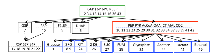
Figure S2: The set of chemicals and reactions, (indicated by numbers) in each box corresponds to a buffering structure with subtraction of its inner buffering structures.

We write down explicitly the 17 buffering structures:

$\Gamma_{1}=(\{\rm Glucose\},\{1\})$.

$\Gamma_{2}=(\{\rm 3PG\},\{8\})$

$\Gamma_{3}=(\{\rm CIT\},\{24\})$,

$\Gamma_{4}=(\{\rm 2{\rm\mathchar 45\relax KG}\},\{26\})$,

$\Gamma_{5}=(\{\rm SUC\},\{27\})$,

$\Gamma_{6}=(\{\rm FUM\},\{28\})$,

$\Gamma_{7}=(\{\rm Glyoxylate\},\{35\})$,

$\Gamma_{8}=(\{\rm Acetate\},\{44\})$,

$\Gamma_{9}=(\{\rm Lactate\},\{45\})$,

$\Gamma_{10}=(\{\rm Ethanol\},\{46\})$,

$\Gamma_{11}=(\{\rm Glucose,PEP,3PG,PYR,AcCoA,OAA,CIT,ICT,\\ 2{\rm\mathchar 45\relax KG},SUC,FUM,MAL,CO2,Glyoxylate,Acetate,Lactate,\\ Ethanol\},\{1,8,9,10,11,12,23,24,25,26,27,28,29,30,31,\\ 32,33,34,35,37,38,39,41,42,44,45,46\})$,

$\Gamma_{12}=(\{\rm X5P,S7P,E4P\},\{17,18,19,20,21\})$,

$\Gamma_{13}=(\{\rm G3P,X5P,S7P,E4P\},\{7,17,18,19,20,21,22\})$

$\Gamma_{14}=(\{\rm X5P,R5P,S7P,E4P\},\{17,18,19,20,21,40\})$,

$\Gamma_{15}=(\{\rm F1,6P\},\{5\})$,

$\Gamma_{16}=(\{\rm DHAP\},\{6\})$,

$\Gamma_{17}=(\{\rm Glucose,PEP,G6P,F6P,F1,6P,DHAP,G3P,3PG,\\ PYR,6PG,Ru5P,X5P,R5P,S7P,E4P,AcCoA,OAA,CIT,\\ ICT,2{\rm\mathchar 45\relax KG},SUC,FUM,MAL,CO2,Glyoxylate,Acetate,\\ Lactate,Ethanol\},\{1,2,3,4,5,6,7,8,9,10,11,12,13,14,15,\\ 16,17,18,19,20,21,22,23,24,25,26,27,28,29,30,31,32,33,\\ 34,35,36,37,38,39,40,41,42,44,45,46\})$.

F.3 Structural bifurcation analysis

For the E. coli system, we construct the matrix A. Up to a constant factor, the determinant ${\rm det}\,{\bf A}$ is factorized as

$${\rm det}\,{\bf A}= r_{1,\text{Glucose}}\,r_{5,\text{F1,6P}}\,r_{6,\text{DHAP}}\,r_{8,\text{3PG}}\,r_{44,\text{Acetate}}\,r_{45,\text{Lactate}}\,r_{46,\text{Ethanol}}$$

$$\times r_{24,\text{CIT}}\,r_{26,\text{2-KG}}\,r_{27,\text{SUC}}\,r_{28,\text{FUM}}\,r_{35,\text{Glyoxylate}}$$

$$\times r_{7,\text{G3P}}\,r_{40,\text{R5P}}\,\left(r_{17,\text{X5P}}r_{19,\text{S7P}}r_{21,\text{E4P}}+r_{18,\text{S7P}}r_{20,\text{E4P}}r_{21,\text{X5P}}\right)$$

$$\times {\rm det}\,{\bf A}_{\Gamma^{\prime}}\times{\rm det}\,{\bf A}_{\Gamma^{\prime\prime}}$$

Here, $r_{n,m}=\frac{\partial r_{n}}{\partial x_{m}}|_{\mbox{\boldmath$x$}=\mbox{\boldmath$x$}^{*}}$. Each of the 17 factors in (LABEL:detAec) is associated with a subnetwork in Fig. S2. Here, the first two lines is the product of the factors ${\rm det}\,{\bf A}_{\Gamma_{s}}$($s=1,3,4,6,9,10,$ $11,12,13,15,16,17$), each of which is associated with a buffering structure $\Gamma_{s}$ with a single chemical. In the third line, $r_{7,\text{G3P}}$, $r_{40,\text{R5P}}$, and the factor inside (…) are associated with the three subnetworks, $(\{{\rm G3P}\},\{7\})$, $(\{{\rm R5P}\},\{40\})$, and $\Gamma_{12}=(\{{\rm X5P,S7P,E4P}\},\{17,18,19,20,21,22\})$ in Fig S2, respectively. The factor ${\rm det}\,{\bf A}_{\Gamma^{\prime}}$ in the last line of (LABEL:detAec) is associated with the subnetwork $\Gamma^{\prime}:=(\{{\rm G6P,F6P,6PG,Ru5P}\},\{2,3,4,13,14,15,16,36,43\})$ (the green box in Fig. S2) and given by

$${\rm det}\,{\bf A}_{\Gamma^{\prime}} =r_{2,\text{G6P}}r_{4,\text{F6P}}\left(r_{15,\text{Ru5P}}+r_{16,\text{Ru5P}}\right)\left(r_{14,\text{6PG}}+r_{36,\text{6PG}}\right)$$

$$+r_{13,\text{G6P}}\biggl{(}r_{4,\text{F6P}}\left(r_{15,\text{Ru5P}}+r_{16,\text{Ru5P}}\right)\left(r_{14,\text{6PG}}+r_{36,\text{6PG}}\right)$$

$$+r_{3,\text{F6P}}\bigl{(}r_{14,\text{6PG}}r_{16,\text{Ru5P}}+\left(r_{15,\text{Ru5P}}+r_{16,\text{Ru5P}}\right)r_{36,\text{6PG}}\bigr{)}\biggr{)}.$$ (122)

The last factor ${\rm det}\,{\bf A}_{\Gamma^{\prime\prime}}$ in (LABEL:detAec) is associated with the subnetwork $\Gamma^{\prime\prime}:=(\{{\rm PEP,PYR,AcCOA,OAA,}$ ${\rm ICT,MAL,CO2}\},$ $\{10,11,12,23,25,29,30,31,32,33,34,37,38,39,41,42\})$ (the red box in Fig. S2) and given by

$${\rm det}\,{\bf A}_{\Gamma^{\prime\prime}} =r_{10,\text{PEP}}(r_{38,\text{PYR}}(r_{23,\text{OAA}}(r_{37,\text{AcCoA}}+r_{39,\text{AcCoA}})(r_{25,\text{ICT}}(2r_{29,\text{MAL}}r_{31,\text{CO2}}$$

$$+r_{33,\text{MAL}}(2r_{31,\text{CO2}}-r_{42,\text{CO2}})+r_{34,\text{ICT}}(r_{33,\text{MAL}}(r_{31,\text{CO2}}-r_{42,\text{CO2}})+r_{29,\text{MAL}}(r_{31,\text{CO2}}+r_{42,\text{CO2}})))$$

$$-(r_{23,\text{AcCoA}}(r_{25,\text{ICT}}+2r_{34,\text{ICT}})+(r_{25,\text{ICT}}+r_{34,\text{ICT}})(r_{37,\text{AcCoA}}+r_{39,\text{AcCoA}}))(r_{29,\text{MAL}}(r_{31,\text{CO2}}r_{41,\text{OAA}}$$

$$+(r_{32,\text{OAA}}+r_{41,\text{OAA}})r_{42,\text{CO2}})+r_{33,\text{MAL}}(r_{31,\text{CO2}}r_{41,\text{OAA}}+(r_{30,\text{OAA}}+r_{32,\text{OAA}}+r_{41,\text{OAA}})r_{42,\text{CO2}})))$$

$$+r_{12,\text{PYR}}(-(r_{25,\text{ICT}}+r_{34,\text{ICT}})(r_{37,\text{AcCoA}}+r_{39,\text{AcCoA}})(r_{29,\text{MAL}}(2r_{31,\text{CO2}}r_{41,\text{OAA}}$$

$$+(r_{32,\text{OAA}}+r_{41,\text{OAA}})r_{42,\text{CO2}})+r_{33,\text{MAL}}(2r_{31,\text{CO2}}r_{41,\text{OAA}}+(r_{30,\text{OAA}}+r_{32,\text{OAA}}+r_{41,\text{OAA}})r_{42,\text{CO2}}))$$

$$+r_{23,\text{OAA}}(r_{37,\text{AcCoA}}+r_{39,\text{AcCoA}})(r_{25,\text{ICT}}(2r_{29,\text{MAL}}r_{31,\text{CO2}}+r_{33,\text{MAL}}(2r_{31,\text{CO2}}-r_{42,\text{CO2}}))$$

$$+r_{34,\text{ICT}}(r_{33,\text{MAL}}(2r_{31,\text{CO2}}-r_{42,\text{CO2}})+r_{29,\text{MAL}}(2r_{31,\text{CO2}}+r_{42,\text{CO2}})))$$

$$-r_{23,\text{AcCoA}}(r_{25,\text{ICT}}(r_{33,\text{MAL}}(4r_{31,\text{CO2}}r_{41,\text{OAA}}+(r_{30,\text{OAA}}$$

$$+r_{32,\text{OAA}})r_{42,\text{CO2}})+r_{29,\text{MAL}}(4r_{31,\text{CO2}}r_{41,\text{OAA}}+(r_{32,\text{OAA}}+r_{41,\text{OAA}})r_{42,\text{CO2}}))$$

$$+r_{34,\text{ICT}}(r_{33,\text{MAL}}(4r_{31,\text{CO2}}r_{41,\text{OAA}}+(r_{30,\text{OAA}}+r_{32,\text{OAA}})r_{42,\text{CO2}})$$

$$+r_{29,\text{MAL}}(4r_{31,\text{CO2}}r_{41,\text{OAA}}+(r_{32,\text{OAA}}+2r_{41,\text{OAA}})r_{42,\text{CO2}})))))$$

$$-r_{31,\text{PEP}}(-r_{11,\text{PYR}}(r_{29,\text{MAL}}+r_{33,\text{MAL}})(r_{23,\text{OAA}}r_{34,\text{ICT}}(r_{37,\text{AcCoA}}+r_{39,\text{AcCoA}})$$

$$-(r_{23,\text{AcCoA}}(r_{25,\text{ICT}}+2r_{34,\text{ICT}})+(r_{25,\text{ICT}}+r_{34,\text{ICT}})(r_{37,\text{AcCoA}}+r_{39,\text{AcCoA}}))r_{41,\text{OAA}})$$

$$+r_{38,\text{PYR}}(r_{23,\text{AcCoA}}(r_{25,\text{ICT}}+2r_{34,\text{ICT}})(r_{30,\text{OAA}}r_{33,\text{MAL}}+(r_{29,\text{MAL}}+r_{33,\text{MAL}})r_{41,\text{OAA}})$$

$$+(r_{37,\text{AcCoA}}+r_{39,\text{AcCoA}})(r_{23,\text{OAA}}(r_{25,\text{ICT}}r_{33,\text{MAL}}+(r_{33,\text{MAL}}-r_{29,\text{MAL}})r_{34,\text{ICT}})$$

$$+(r_{25,\text{ICT}}+r_{34,\text{ICT}})(r_{30,\text{OAA}}r_{33,\text{MAL}}+(r_{29,\text{MAL}}+r_{33,\text{MAL}})r_{41,\text{OAA}})))$$

$$+r_{12,\text{PYR}}(r_{23,\text{AcCoA}}(r_{25,\text{ICT}}(r_{30,\text{OAA}}r_{33,\text{MAL}}$$

$$+r_{29,\text{MAL}}r_{41,\text{OAA}})+r_{34,\text{ICT}}(r_{30,\text{OAA}}r_{33,\text{MAL}}+2r_{29,\text{MAL}}r_{41,\text{OAA}}))+(r_{37,\text{AcCoA}}$$

$$+r_{39,\text{AcCoA}})(r_{23,\text{OAA}}(r_{25,\text{ICT}}r_{33,\text{MAL}}+(r_{33,\text{MAL}}-r_{29,\text{MAL}})r_{34,\text{ICT}})$$

$$+(r_{25,\text{ICT}}+r_{34,\text{ICT}})(r_{30,\text{OAA}}r_{33,\text{MAL}}+(r_{29,\text{MAL}}+r_{33,\text{MAL}})r_{41,\text{OAA}}))))r_{42,\text{CO2}}.$$ (123)

Since $r_{n,m}>0$, we see that, among the 17 factors in (LABEL:detAec), only the last factor ${\rm det}\,{\bf A}_{\Gamma^{\prime\prime}}$ contains both of plus and minus signs. Therefore, if this system exhibits a steady-state bifurcation (under parameter change), it should be the subnetwork $\Gamma^{\prime\prime}$ whose determinant changes its sign at the bifurcation point.

F.4 Numerical analysis

In the discussion so far, we have not assumed any specific kinetic for reaction rates. To numerically demonstrate bifurcation behaviors in the E. coli system, we first consider the case that all the reactions obey the mass-action kinetics with reaction rate constant $k_{n}$ $(n=1,\ldots,47)$. In this case, we found that, for any parameter choices, the E. coli system has either a single stable solution or a blow up solution, and no steady-state bifurcations were observed. We also performed the same analysis in the case of the Michaelis-Menten kinetics, and no bifurcations were observed.

We next consider the case that the reaction 11 : $\rm PYR\rightarrow\rm PEP$ is positively regulated by PEP. Specifically, we modified the rate of reaction 11 from $r_{11}=k_{11}x_{\rm PYR}$ into

$$r_{11}=k_{11}x_{\rm PYR}\biggl{(}1+k_{11,PEP}\frac{x_{\rm PEP}^{2}}{x_{\rm PEP}^{2}+K}\biggr{)}$$ (124)

where $k_{11,\rm PEP}$ represents the strength of the regulation. All reactions except reaction 11 obey the mass-action kinetics as before.

We remark that the regulation from PEP to reaction 11 does not change the buffering structures in section F.2 since adding this regulation does not ruin the condition of output-completeness. Thus, the inclusion relation of buffering structures shown in Fig. F.2 is also intact under the modification (124) of the kinetics.

As explained previously, only bifurcations associated with $\Gamma^{\prime\prime}$ (the red box in Fig S2) are possible for this system. The inducing parameters are then given by parameters associated with reactions in the green and red boxes in Fig S2. As a candidate bifurcation parameter, we choose the parameter $k_{11,PEP}$, which is associated with reaction 11 and an inducing parameter for $\Gamma^{\prime\prime}$. The reaction rate constants of the mass-action kinetics were set as

$$(k_{1},\ldots,k_{47}) =(18.9,\,55.9,\,20.5,\,5.17,\,8.14,\,107,\,15.7,\,2.38,\,32,\,3.08,\,$$

$$38.8,\,471,\,7.54,\,1.28,\,24.4,\,84.9,\,23.1,\,1.64,\,90.6,\,132,\,$$

$$65,\,47,\,237,\,1.19,\,11.7,\,1.80,\,98.5,\,27,\,1090,\,3.15,\,$$

$$484,\,1.44,\,543,\,12.2,\,20,\,89.5,\,2.98,\,7.23,\,48.9,\,2.96,\,$$

$$21.6,\,37.6,\,85,\,131,\,28.2,\,2.37).$$ (125)

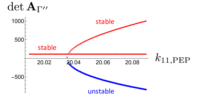
Figure S3: ${\rm det}\,{\bf A}_{\Gamma^{\prime\prime}}$ versus $k_{11,PEP}$. The red curves correspond to two stable solutions, and the blue curve corresponds to an unstable solution.

Fig. S3 shows the numerical result for ${\rm det}\,{\bf A}_{\Gamma^{\prime\prime}}$ versus $k_{11,PEP}$. For large $k_{11,PEP}$, there are two stable solutions (red curves) and one unstable solution (blue curve). As $k_{11,PEP}$ is decreased, the values of ${\rm det}\,{\bf A}_{\Gamma^{\prime\prime}}$ for a stable and unstable solutions decreases and eventually approach zero. Thus, the parameter $k_{11,PEP}$, which is one of the inducing parameters for $\Gamma^{\prime\prime}$, actually induces a bifurcation associated with $\Gamma^{\prime\prime}$.

The bifurcating chemicals for $\Gamma^{\prime\prime}$ are those in the blue and red boxes. Fig. S4 shows the numerical results for the steady-state concentrations versus the parameter $k_{11,\rm PEP}$. We see that saddle-node bifurcations are observed only for the bifurcating chemicals.

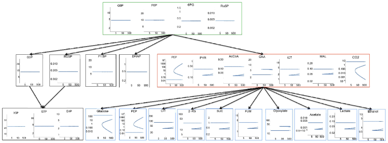
Figure S4: Steady-state concentrations versus $k_{11,\rm PEP}$ (the horizontal axis) in the E. coli system. Each box corresponds to the one in Fig. S2. A saddle-node bifurcation is observed for each of the bifurcating chemicals (the red and blue boxes) for $\Gamma^{\prime\prime}$: Each chemical in the red and blue boxes has one stable branch when $k_{11,\rm PEP}$ is small, and has two stable and one unstable branches when $k_{11,\rm PEP}$ is large. Each chemical in the green and black boxes is independent of $k_{11,\rm PEP}$, due to the law of localization, and has one stable branch.

Appendix G An example exhibiting transcritical bifurcation

Consider the system in Fig. S5. This system is designed by modifying the First Schlögl Model schlogl .

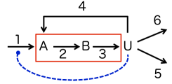
Figure S5: System consisting of six reactions, ${\rm U}\overset{k_{1}}{\rightarrow}{\rm U+A},\ {\rm A}\overset{k_{2}}{\rightarrow}{\rm B},{\rm B}\overset{k_{3}}{\rightarrow}{\rm U},\ {\rm U}\overset{k_{4}}{\rightarrow}{\rm A},2{\rm U}\overset{k_{5}}{\rightarrow}{\rm U},\ {\rm U}\overset{k_{6}}{\rightarrow}$. The red box indicates a buffering structure.

It consists of reactions

$${\rm U}\overset{k_{1}}{\rightarrow}{\rm U+A},\ {\rm A}\overset{k_{2}}{\rightarrow}{\rm B},\ {\rm B}\overset{k_{3}}{\rightarrow}{\rm U},\ {\rm U}\overset{k_{4}}{\rightarrow}{\rm A},$$

$$2{\rm U}\overset{k_{5}}{\rightarrow}{\rm U}, \ {\rm U}\overset{k_{6}}{\rightarrow}.$$ (126)

The stoichiometry matrix $\nu$ is

$$\nu=\left(\begin{array}[]{cccccc}1&-1&0&1&0&0\\ 0&1&-1&0&0&0\\ 0&0&1&-1&-1&-1\\ \end{array}\right),$$ (130)

which has three independent kernel vectors ${\mbox{\boldmath$c$}}_{1}=(1,1,1,0,0,1)^{T},{\mbox{\boldmath$c$}}_{2}=(1,1,1,0,1,0)^{T},{\mbox{\boldmath$c$}}_{3}=(0,1,1,1,0,0)^{T}$.

The system contains a buffering structure ${\Gamma_{s}}=(\{{\rm A,B}\},\{2,3\})$, since $\chi=2-2+0=0$. By permutating the row index as $\{2,3,1,4,5,6\}$ and the column index as $\{\text{A},\text{ B},\text{ U},{\mbox{\boldmath$c$}}_{1},{\mbox{\boldmath$c$}}_{2},{\mbox{\boldmath$c$}}_{3}\}$, we obtain

$${\bf A}=\left(\begin{array}[]{cccccc}\cline{1-2}\cr\vrule\lx@intercol\hfil r_{2,\text{A}}\hfil\lx@intercol&\lx@intercol\hfil 0\hfil\lx@intercol\vrule\lx@intercol&0&1&1&1\\ \vrule\lx@intercol\hfil 0\hfil\lx@intercol&\lx@intercol\hfil r_{3,\text{B}}\hfil\lx@intercol\vrule\lx@intercol&0&1&1&1\\ \cline{1-6}\cr 0&0&\vrule\lx@intercol\hfil r_{1,\text{U}}\hfil\lx@intercol&1&1&\lx@intercol\hfil 0\hfil\lx@intercol\vrule\lx@intercol\\ 0&0&\vrule\lx@intercol\hfil r_{4,\text{U}}\hfil\lx@intercol&0&0&\lx@intercol\hfil 1\hfil\lx@intercol\vrule\lx@intercol\\ 0&0&\vrule\lx@intercol\hfil r_{5,\text{U}}\hfil\lx@intercol&0&1&\lx@intercol\hfil 0\hfil\lx@intercol\vrule\lx@intercol\\ 0&0&\vrule\lx@intercol\hfil r_{6,\text{U}}\hfil\lx@intercol&1&0&\lx@intercol\hfil 0\hfil\lx@intercol\vrule\lx@intercol\\ \cline{3-6}\cr\end{array}\right),$$ (137)

where the upper-left block and the lower-right block correspond to $\bf A_{{\Gamma_{s}}}$ and $\bf A_{\bar{\Gamma}_{s}}$, respectively. Thus, the determinant becomes

$${\rm det}\,{\bf A}=\underset{{\rm det}\,{\bf A}_{\Gamma_{s}}}{\underbrace{r_{2,\text{A}}r_{3,\text{B}}}}\underset{{\rm det}\,{\bf A}_{\bar{\Gamma}_{s}}}{\underbrace{\left(-r_{1,\text{U}}+r_{5,\text{U}}+r_{6,\text{U}}\right)}}.$$ (138)

Thus, a steady-state bifurcation can occur when ${\rm det}\,{\bf A}_{\bar{\Gamma}_{s}}$ changes its sign.

G.1 The mass-action kinetics case

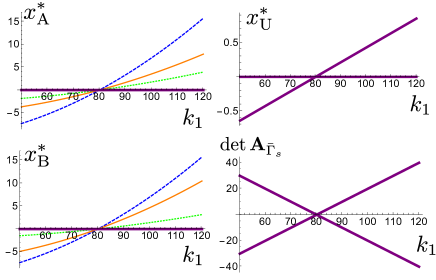
Figure S6: Concentrations and ${\rm det}\,{\bf A}_{\bar{\Gamma}_{s}}$ for different values of $(k_{2},k_{3})$. All three cases have the solution ${\mbox{\boldmath$x$}}^{*}={\mbox{\boldmath$0$}}$. The dashed blue line, the solid orange line, and the dotted green line correspond to $(k_{2},k_{3})=(10,10),\ (20,15),\ (40,50)$, while $(k_{4},k_{5},k_{6})$ are fixed as $(k_{4},k_{5},k_{6})$$=(65,47,80)$ in all of the three cases. The solid purple lines indicate that the plots for these three parameter choices coincide with each other.

The inducing parameters for ${\bar{\Gamma}_{s}}$ are those associated with reaction in ${\bar{\Gamma}_{s}}$, that is, $\{k_{1},k_{4},k_{5},k_{6}\}$. Fig. S6 shows the bifurcation diagram, where the mass-action kinetics is assumed as in schlogl . The determinant ${\rm det}\,{\bf A}_{\bar{\Gamma}_{s}}$ and the steady-state concentrations versus the parameter $k_{1}$ are shown for three different sets of parameters inside ${\Gamma_{s}}$, i.e. $k_{2},k_{3}$. From the plots for ${\rm det}\,{\bf A}_{\bar{\Gamma}_{s}}$, we see the parameter $k_{1}$, which is an inducing parameter for ${\bar{\Gamma}_{s}}$, actually induces the bifurcation associated with ${\bar{\Gamma}_{s}}$.

As for steady-state concentrations, the bifurcations are observed in all chemicals in the system, since the bifurcating chemicals for $\bar{\Gamma}_{s}$ are all chemicals. In the plots for concentrations in Fig. S6, we see that, for small $k_{1}$, the system has a single stable solution ${\bm{x}}^{*}=\bm{0}$ and an (unphysical negative) unstable solution. For large $k_{1}$, the former becomes an unstable solution and the latter becomes a positive stable solution. Thus, the system in Fig. S6 exhibits the transcritical bifurcation. We can also see that both steady-state value of $x_{\rm U}^{*}$ and the critical value of $k_{1}\in{\bar{\Gamma}_{s}}$ are independent of parameters inside $\Gamma_{s}$.

In the case of the mass-action kinetic, we can explicitly obtain the analytic solutions. Indeed, the steady state is given by

$$(x^{*}_{A},x^{*}_{B},x^{*}_{U})=(0,0,0),\quad\bigl{(}\frac{(k_{1}+k_{4})(k_{1}-k_{6})}{k_{2}k_{5}},\frac{(k_{1}+k_{4})(k_{1}-k_{6})}{k_{3}k_{5}},\frac{k_{1}-k_{6}}{k_{5}}\bigr{)},$$ (139)

and the determinant of A is given by

$${\rm det}\,{\bf A}=\underset{{\rm det}\,{\bf A}_{\Gamma_{s}}}{\underbrace{k_{2}k_{3}}}\underset{{\rm det}\,{\bf A}_{\bar{\Gamma}_{s}}}{\underbrace{\left(-2k_{5}x^{*}_{\text{U}}+k_{1}-k_{6}\right)}}=\pm k_{2}k_{3}(k_{1}-k_{6}),$$ (140)

where $+$ and $-$ corresponds to the first and the second solution in (139), respectively. The critical point is given by $k_{1}=k_{6}$, which is indeed independent of $k_{2},k_{3}\in{\Gamma_{s}}$.

G.2 The modified mass-action kinetics case

Finally, we show the result for a more complicated kinetics. Specifically, instead of the mass-action kinetics, we consider the following reaction rate functions,

$$(r_{1},\ldots,r_{6})=\left(k_{1}x_{\text{U}},k_{2}x_{\text{A}}\left(1+\frac{k_{2,{\rm B}}x^{2}_{\text{B}}}{x^{2}_{\text{B}}+K}\right),k_{3}x_{\text{B}}\left(1+\frac{k_{3,{\rm A}}x^{2}_{\text{A}}}{x^{2}_{\text{A}}+K}\right),k_{4}x_{\text{U}},k_{5}x_{\text{U}}^{2},k_{6}x_{\text{U}}\right)$$ (141)

This system reduces to the case of the mass-action kinetic when $k_{2,{\rm B}}=0$ and $k_{3,{\rm A}}=0$.

Fig. S7 shows the numerical results of concentrations and ${\rm det}\,{\bf A}$ for different values of $k_{2,B}$ and $k_{3,A}$. For the plot of the curve of filled circle, $k_{2,B}=5$ and $k_{3,A}=5$. For the plot of the curve of empty circle, $k_{2,B}=10$ and $k_{3,A}=15$. The other parameters are the same for the two plots; $(k_{1},\ldots,k_{6})=(40,10,80,70,90,10)$ and $K=5$. Note that only non-negative physical solutions are shown in Figure S7. We observe that the qualitative behavior is the same as the case of the mass-action kinetics: $x^{*}_{{\rm U}}$, ${\rm det}\,{\bf A}_{\bar{\Gamma}}$, and the critical value of $k_{1}$ is independent of the parameters inside the buffering structure. On the other hand, the positive solutions of $x^{*}_{{\rm A}}$ and $x^{*}_{{\rm B}}$ depend on these parameters.

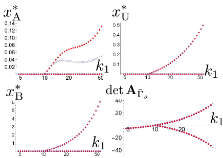
Figure S7: Concentrations and ${\rm det}\,{\bf A}_{{\bar{\Gamma}_{s}}}$ for different values of $k_{2,B}$ and $k_{3,A}$. The solution ${\mbox{\boldmath$x$}}^{*}=0$ exists for all parameters. The plots for A, B $\in{\Gamma_{s}}$ depend on the parameters $k_{2,B},k_{3,A}\in{\Gamma_{s}}$, while those of ${\rm U}\in{\bar{\Gamma}_{s}}$ and ${\rm det}\,{\bf A}_{\bar{\Gamma}_{s}}$ do not.

Appendix H Example network with $K_{c}>0$

The following system is known to exhibit a saddle-node bifurcation, when mass-action kinetics is assumed CC .

$$\text{A}+\text{E1} \underset{2}{\overset{1}{\rightleftharpoons}}\text{ AE1}$$

AE1 $$\overset{3}{\rightarrow}\text{Ap + E1}$$

Ap + E1 $$\underset{5}{\overset{4}{\rightleftharpoons}}\text{ApE1}$$

ApE1 $$\overset{6}{\rightarrow}\text{App + E1}$$

App + E2 $$\underset{8}{\overset{7}{\rightleftharpoons}}\text{ AppE2}$$

AppE2 $$\overset{9}{\rightarrow}\text{Ap + E2}$$

Ap + E2 $$\underset{11}{\overset{10}{\rightleftharpoons}}\text{ApE2}$$

ApE2 $$\overset{12}{\rightarrow}\text{A + E2}$$ (142)

Here, we consider an extended system by coupling the above system (142) with the following four reactions,

Ap + B $$\underset{14}{\overset{13}{\rightleftharpoons}}\text{A + Bp}$$

B + F $$\underset{16}{\overset{15}{\rightleftharpoons}}\text{BF }$$ (143)

In this extended system, the extended part $\Gamma_{s}=\text{(B,Bp,F,13,14,15,16)}$ is a buffering structure because $\chi=3-4+2-1$. The complement subnetwork ${\bar{\Gamma}_{s}}$ in the extended system consists of all the chemicals and reactions existing in the original system.

The stoichiometry matrix is given by

$$\nu=\left(\begin{array}[]{cccccccccccccccc}-1&1&0&0&0&0&0&0&0&0&0&1&1&-1&0&0\\ -1&1&1&-1&1&1&0&0&0&0&0&0&0&0&0&0\\ 1&-1&-1&0&0&0&0&0&0&0&0&0&0&0&0&0\\ 0&0&1&-1&1&0&0&0&1&-1&1&0&-1&1&0&0\\ 0&0&0&1&-1&-1&0&0&0&0&0&0&0&0&0&0\\ 0&0&0&0&0&1&-1&1&0&0&0&0&0&0&0&0\\ 0&0&0&0&0&0&-1&1&1&-1&1&1&0&0&0&0\\ 0&0&0&0&0&0&1&-1&-1&0&0&0&0&0&0&0\\ 0&0&0&0&0&0&0&0&0&1&-1&-1&0&0&0&0\\ 0&0&0&0&0&0&0&0&0&0&0&0&-1&1&-1&1\\ 0&0&0&0&0&0&0&0&0&0&0&0&1&-1&0&0\\ 0&0&0&0&0&0&0&0&0&0&0&0&0&0&-1&1\\ 0&0&0&0&0&0&0&0&0&0&0&0&0&0&1&-1\\ \end{array}\right),$$ (157)

where the column indices from left to right are

$$\{\text{A},\text{E1},\text{AE1},\text{Ap},\text{ApE1},\text{App},\text{E2},\text{AppE2},\text{ApE2},\text{B},\text{Bp},\text{F},\text{BF}\}.$$ (158)

We represent the rate constants for the twelve reactions in (142) as $k_{1},\ldots k_{12}$, and the four reactions in (143) as $k_{13},\ldots k_{16}$. For example, the rate functions of the first and the second reaction are $R_{1}=k_{1}x_{A}x_{E1}$ and $R_{2}=k_{2}x_{AE1}$, respectively.

The matrix $\bf A$ is given by

$$\left(\begin{array}[]{ccccccccccccc|cccccccc}k_{1}x_{\text{E1}}&k_{1}x_{\text{A}}&0&0&0&0&0&0&0&0&0&0&0&0&0&1&0&0&0&0&1\\ 0&0&k_{2}&0&0&0&0&0&0&0&0&0&0&0&0&0&0&0&0&0&1\\ 0&0&k_{3}&0&0&0&0&0&0&0&0&0&0&0&0&1&0&0&0&0&0\\ 0&k_{4}x_{\text{Ap}}&0&k_{4}x_{\text{E1}}&0&0&0&0&0&0&0&0&0&0&0&0&0&1&0&1&0\\ 0&0&0&0&k_{5}&0&0&0&0&0&0&0&0&0&0&0&0&0&0&1&0\\ 0&0&0&0&k_{6}&0&0&0&0&0&0&0&0&0&0&0&0&1&0&0&0\\ 0&0&0&0&0&k_{7}x_{\text{E2}}&k_{7}x_{\text{App}}&0&0&0&0&0&0&0&0&0&0&1&1&0&0\\ 0&0&0&0&0&0&0&k_{8}&0&0&0&0&0&0&0&0&0&0&1&0&0\\ 0&0&0&0&0&0&0&k_{9}&0&0&0&0&0&0&0&0&0&1&0&0&0\\ 0&0&0&k_{10}x_{\text{E2}}&0&0&k_{10}x_{\text{Ap}}&0&0&0&0&0&0&0&0&1&1&0&0&0&0\\ 0&0&0&0&0&0&0&0&k_{11}&0&0&0&0&0&0&0&1&0&0&0&0\\ 0&0&0&0&0&0&0&0&k_{12}&0&0&0&0&0&0&1&0&0&0&0&0\\ 0&0&0&k_{13}x_{\text{B}}&0&0&0&0&0&k_{13}x_{\text{Ap}}&0&0&0&0&1&0&0&0&0&0&0\\ k_{14}x_{\text{Bp}}&0&0&0&0&0&0&0&0&0&k_{14}x_{\text{A}}&0&0&0&1&0&0&0&0&0&0\\ 0&0&0&0&0&0&0&0&0&k_{15}x_{\text{F1}}&0&k_{15}x_{\text{B}}&0&1&0&0&0&0&0&0&0\\ 0&0&0&0&0&0&0&0&0&0&0&0&k_{16}&1&0&0&0&0&0&0&0\\ \\ \hline\cr 1&0&1&1&1&1&0&1&1&0&0&0&0&0&0&0&0&0&0&0&0\\ 0&1&1&0&1&0&0&0&0&0&0&0&0&0&0&0&0&0&0&0&0\\ 0&0&0&0&0&0&1&1&1&0&0&0&0&0&0&0&0&0&0&0&0\\ 0&0&0&0&0&0&0&0&0&1&1&0&1&0&0&0&0&0&0&0&0\\ 0&0&0&0&0&0&0&0&0&0&0&1&1&0&0&0&0&0&0&0&0\\ \end{array}\right),$$ (181)

and the corresponding determinant ${\rm det}\,{\bf A}$ is

$${\rm det}\,{\bf A}= \underset{{\rm det}\,{\bf A}_{\Gamma_{s}}}{\underbrace{\biggl{(}k_{14}x_{\text{A}}(k_{15}(x_{\text{B}}+x_{\text{F1}})+k_{16})+k_{13}x_{\text{Ap}}(k_{15}x_{\text{B}}+k_{16})\biggr{)}}}$$ (182)

$$\times\biggl{(}k_{1}(k_{3}x_{\text{E1}}(k_{4}(k_{7}k_{9}x_{\text{E2}}(k_{10}x_{\text{Ap}}(x_{\text{A}}+x_{\text{Ap}}+x_{\text{App}}+x_{\text{E1}}$$

$$+x_{\text{E2}})+k_{11}(x_{\text{A}}+x_{\text{Ap}}+x_{\text{E1}})+k_{12}(x_{\text{A}}+x_{\text{Ap}}+x_{\text{E1}}))$$

$$+k_{6}x_{\text{E1}}(k_{8}(k_{10}x_{\text{Ap}}+k_{11}+k_{12})+k_{9}(k_{10}x_{\text{Ap}}+k_{11}+k_{12})+k_{7}(k_{11}+k_{12})$$

$$(x_{\text{App}}+x_{\text{E2}})))+(k_{5}+k_{6})k_{7}k_{9}x_{\text{E2}}(k_{10}(x_{\text{Ap}}+x_{\text{App}}+x_{\text{E2}})+k_{11}+k_{12}))$$

$$-k_{10}k_{12}x_{\text{E2}}(k_{4}k_{6}x_{\text{Ap}}x_{\text{E1}}(k_{7}(x_{\text{A}}+x_{\text{Ap}}+x_{\text{App}}+x_{\text{E1}}$$

$$+x_{\text{E2}})+k_{8}+k_{9})-(k_{5}+k_{6})k_{7}k_{9}x_{\text{E2}}(x_{\text{A}}+x_{\text{E1}})))-(k_{2}+k_{3})k_{7}k_{10}k_{12}x_{\text{E2}}$$

$$(k_{4}k_{6}x_{\text{Ap}}x_{\text{E1}}-k_{9}x_{\text{E2}}(k_{4}x_{\text{Ap}}+k_{5}+k_{6}))\biggr{)}.$$ (183)

While the factor ${\rm det}\,{\bf A}_{\Gamma_{s}}$ is positive definite, the factor ${\rm det}\,{\bf A}_{{\bar{\Gamma}_{s}}}$ can change the sign as we change parameters since it contains the negative terms. Therefore, the saddle-node bifurcations can arise from ${\rm det}\,{\bf A}_{\bar{\Gamma}_{s}}$. Furthermore, the factor ${\rm det}\,{\bf A}_{\bar{\Gamma}_{s}}$ is independent of the parameters and concentrations in $\Gamma$, as is ensured from the property of buffering structure. Therefore, the bifurcation points of this extended system are completely the same as the original system (142). Below, we demonstrate these expectations by numerical computation.

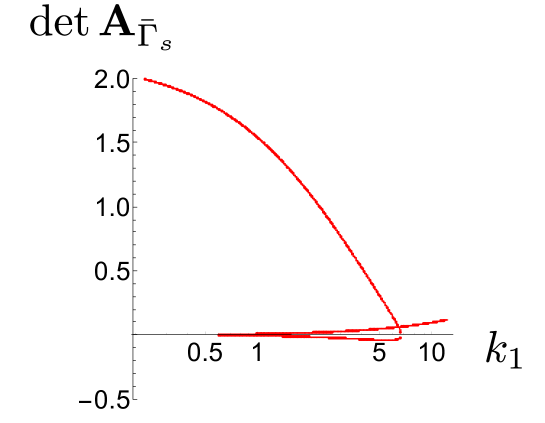
Figure S8: Values of ${\rm det}\bf A_{\bar{\Gamma}_{s}}$ versus $k_{1}$.

The inducing parameters for the subnetwork ${\bar{\Gamma}_{s}}$ are parameters in ${\bar{\Gamma}_{s}}$. Fig. S8 shows that the determinant of $\bf A$ versus the parameter $k_{1}$, which is the parameter in ${\bar{\Gamma}_{s}}$. The other rata parameters are chosen as

$$(k_{2},\ldots,k_{12}) =(30,30,20,2,2,800,1,1,500,14,14),$$

$$(k_{13},\ldots,k_{16}) =(3,2,10,7)$$ (184)

and the values of conserved concentrations are chosen as

$$x_{\text{A}}+x_{\text{AE1}}+x_{\text{Ap}}+x_{\text{ApE1}}+x_{\text{ApE2}}+x_{\text{App}}+x_{\text{AppE2}}=10$$

$$x_{\text{AE1}}+x_{\text{ApE1}}+x_{\text{E1}}=3$$

$$x_{\text{ApE2}}+x_{\text{AppE2}}+x_{\text{E2}}=4$$

$$x_{\text{B}}+x_{\text{BF1}}+x_{\text{Bp}}=6$$

$$x_{\text{BF1}}+x_{\text{F1}}=4.$$ (185)

In Fig. S8, we see that, as we change the parameter $k_{1}$, there are two bifurcation points with ${\rm det}\,{\bf A}_{\bar{\Gamma}_{s}}=0$. Thus, the parameter $k_{1}$ indeed acts as a bifurcation parameter associated with the subnetwork ${\bar{\Gamma}_{s}}$.

The bifurcation chemicals for ${\bar{\Gamma}_{s}}$ are all chemicals in the extended system. This is illustrated in Fig. S9, where the steady-state concentrations for $A,App$ and $Bp$ versus $k_{1}$ are shown. We also see that the original and extended systems have exactly the same critical value of $k_{1}$, as expected. Furthermore, for chemicals existing in the original system (142), or equivalently chemicals in ${\bar{\Gamma}_{s}}$, the plots for the extended system exactly coincides with those in the original system. This can be understood from the law of localization: The original system can be obtained from the extended system, by taking the limit that the parameters in ${\Gamma_{s}}$ (i.e. $k_{13},k_{14},k_{15},k_{16}$) go to zero. However, the chemicals in ${\bar{\Gamma}_{s}}$ are not influenced in the limiting procedure because the law of localization states that changing the parameters in ${\Gamma_{s}}$ does not influence the chemicals in ${\bar{\Gamma}_{s}}$.

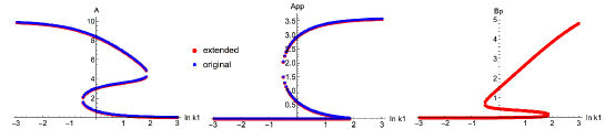
Figure S9: (Left,Center) Steady-state concentrations of $A,App$ for the original and the extended system. (Right) Concentration of $Bp$ in the extended system.

References

- (1) A.A. Andronov, E.A. Leontovich, I.I. Gordon, A.G. Maier, “Theory of bifurcations of dynamical systems on a plane”, Israel Program Sci. Transl. (1971). (In Russian)
- (2) V.I. Arnol’d, “Geometrical methods in the theory of ordinary differential equations” , Grundlehren math. Wiss., 250, Springer (1983). (In Russian)
- (3) J. Carr, ”Applications of center manifold theory”, Springer (1981).
- (4) J. Guckenheimer and Ph. Holmes, ”Nonlinear oscillations, dynamical systems and bifurcations of vector fields”, Springer (1983).
- (5) Klipp, Edda, et al. Systems biology: a textbook. John Wiley & Sons, 2016.
- (6) Yu.A. Kuznetsov, ”Elements of applied bifurcation theory”, Springer (1995).
- (7) Mochizuki, A., Fiedler, B.,Journal of theoretical biology, 367, 189-202 (2015).
- (8) Craciun G., Feinberg M. SIAM J. App. Math. 66:4,1321-1338 (2006).
- (9) Feinberg M. Arch. Rational Mech. Anal. 132, 311-370 (1995) .
- (10) T. Okada and A. Mochizuki, Phys. Rev. Lett. 117.4 (2016), 048101.
- (11) T. Okada and A. Mochizuki, Phys. Rev. E 96, 022322.
- (12) F. Schlögl, Zeitschrift für Physik A Hadrons and Nuclei 253.2 (1972): 147-161.
- (13) Conradi, Carsten, Dietrich Flockerzi, and Jorg Raisch. American Control Conference, 2007. ACC’07. IEEE, 2007.
- (14) Klipp, Edda, et al. Systems biology: a textbook. John Wiley & Sons, 2016.
- (15) A. Vanderbauwhede, Centre manifolds, normal forms and elementary bifurcations, Dynamics Reported, 2 (1989,) pp. 89–169.
- (16) D.C. Whitley, Discrete dynamical systems in dimensions one and two, Bull. London Math. Soc. , 15 (1983), pp. 177–217.