Atomistic potential for graphene and other sp² carbon systems

Abstract

We introduce a torsional force field for sp² carbon to augment an in-plane atomistic potential of a previous work (Kalosakas et al, J. Appl. Phys. 113, 134307 (2013)) so that it is applicable to out-of-plane deformations of graphene and related carbon materials. The introduced force field is fit to reproduce DFT calculation data of appropriately chosen structures. The aim is to create a force field that is as simple as possible so it can be efficient for large scale atomistic simulations of various sp² carbon structures without significant loss of accuracy. We show that the complete proposed potential reproduces characteristic properties of fullerenes and carbon nanotubes. In addition, it reproduces very accurately the out-of-plane ZA and ZO modes of graphene’s phonon dispersion as well as all phonons with frequencies up to 1000 cm^-1.

I Introduction

Carbon nanostructures with predominant sp² bonds, like carbon fullerenes, nanotubes (CNTs) and graphene, are in the center of scientific and technological interest for more than three decades Kroto et al. (1985); Iijima (1991); Novoselov et al. (2004). This interest has increased significantly after the synthesis and identification of single layer graphene which has triggered an unprecedented focus of research on the material itself, its potential applications and other two-dimensional materials Castro Neto et al. (2009); Ferrari (2007); Ferrari et al. (2015); Zhu et al. (2010); Geim and Grigorieva (2013); Bhimanapati et al. (2015). The accurate, yet efficient, modeling of sp² bonded carbon at an atomistic level remains a great challenge for theory. Although there exist several atomistic models Tersoff (1988, 1989); Lindsay and Broido (2010); Brenner (1990); Senftle et al. (2016); Srinivasan et al. (2015); Los and Fasolino (2003); Los et al. (2005); Stuart et al. (2000); Wei et al. (2011) and many of them have been proven accurate in describing several properties of carbon based nanomaterials at a microscopic level, there is a continuous need for as simple as possible and at the same time as accurate as possible models that could allow the simulation at a large, and increasing, scale Fasolino et al. (2007); Zakharchenko et al. (2009); Zhao et al. (2009); Xu and Buehler (2010); Neek-Amal and Peeters (2010); Sgouros et al. (2014); Fthenakis and Tománek (2012); Zhang et al. (2014); Fthenakis and Lathiotakis (2015); Yoon et al. (2016); Sgouros et al. (2016); Meng et al. (2017); Jain et al. (2017).

In a previous work Kalosakas et al. (2013), a force field for graphene was presented with terms depending only on atomic displacements within the graphene plane. In the present work, we extend that potential with the inclusion of torsional terms. The improvement achieved with these new terms is that it can be used to describe accurately out-of-plane distortions. For validation, we apply the present potential to several characteristic test cases like the relative stability of fullerene isomers, the strain energy and the Young’s modulus of CNTs and the phonon dispersion of graphene.

The potential energy in atomistic simulations can be approximately expressed as the sum of several terms corresponding to specific geometric deformations originating from covalent, electrostatic or weak interactions. In the present, for $sp^{2}$ carbon systems, we consider only terms arising from covalent bonding. Electrostatic terms are excluded since there is no charge localization on atoms, while for a single layer of sp² carbon atoms weak interactions can be neglected. Therefore, we assume a deformation energy $U$ of the form

$$U=U_{\rm str}+U_{\rm bend}+U_{\rm tors}$$ (1)

where $U_{\rm str}$ is a bond-stretching term, $U_{\rm bend}$ an angle-bending term and $U_{\rm tors}$ a term depending on out-of-plane torsional angle deformations. In a previous work Kalosakas et al. (2013), parametric forms for the first two terms were presented, derived through fitting to ab-initio calculations. The individual (for a single bond or angle) bond-stretching and angle-bending terms, i.e. the contributions to $U_{\rm str}$ and $U_{\rm bend}$ corresponding to a single bond or angle distortion, have respectively the forms Kalosakas et al. (2013)

$$V_{s}(r)=D\left[e^{-a(r-r_{0})}-1\right]^{2}\,,$$ (2)

with parameters $D=5.7\;eV$, $a=1.96$ Å^-1, and $r_{0}=1.42$ Å, and

$$V_{b}(\theta)=\frac{k}{2}\left(\theta-\frac{2\pi}{3}\right)^{2}-\frac{k^{\prime}}{3}\left(\theta-\frac{2\pi}{3}\right)^{3}\,,$$ (3)

with $k=7.0\;{\rm eV}/{\rm rad}^{2}$ and $k^{\prime}=4\;{\rm eV}/{\rm rad}^{3}$. Then the deformation energy terms of Eq. (1) are $U_{\rm str}=\sum_{i}V_{s}(r_{i})$ and $U_{\rm bend}=\sum_{j}V_{b}(\theta_{j})$, with $i$ and $j$ enumerating all the different bonds and angles, respectively.

This potential was proven useful in several cases, for example in reproducing accurately several elastic properties of graphene Kalosakas et al. (2013). However, it is only applicable to cases for which no out-of-plane deformations occur. For out-of-plane distortions, the bond-stretching and angle-bending terms alone are not sufficient to yield accurate results and augmentation of the force-field with torsional terms is required (see for instance the discussion for C₄₀ isomers in Sec. III.1). This is the main task of this work. Following the same recipe as in Ref. Kalosakas et al., 2013 we assume a simple form for the individual torsional term with parameters that are fitted to reproduce deformation energies from ab-initio calculations. Our aim is to keep the potential as simple as possible, so it can be used in large scale molecular dynamics or Monte Carlo atomistic simulations in graphene and other sp² carbon materials, being at the same time as accurate as possible.

In order to check the efficiency of the proposed potential, we implemented it in LAMMPS computer codePlimpton (1995); lam and tested its speed compared with two popular atomistic models, namely Tersoff-2010Lindsay and Broido (2010), and LCBOP Los and Fasolino (2003). We simulated graphene with periodic boundary conditions assuming a cell of 1152 atoms. We found that our scheme is 3 and 4 times faster in this simulation than Tersoff-2010 and LCBOP, respectively. Thus, the present potential will be a very good choice for extended sp² carbon systems. In case local phenomena are under study, for instance functionalization of such systems, then one expects that locally the structures depart from sp² hybridization. In that case, the potential can be either modified locally to account more accurately for such effects, or replaced locally by a more accurate, but likely less effective scheme.

This paper is organized as follows: In Section II, we describe the additional torsional terms and the procedure of fitting, i.e. optimizing the associated parameters. Full details for this procedure are given in a separate report Chatzidakis et al. . Then, in Section III, we demonstrate the efficiency and the accuracy of this potential in specific applications: energetics of fullerenes (Sec. III.1), the strain energy and the Young’s modulus of CNTs (Sec. III.2), and the phonon dispersion of graphene (Sec. III.3). Conclusions are included in Sec. IV.

II Torsional Force Field

In order to fit the parameters of a torsional term, we calculated ab-initio the total energies of two structures of a single graphene layer folded by an angle $\phi$ around an axis lying along either an armchair or a zig-zag direction. These structures are shown in Fig. 1 and the corresponding unit cells are also included. The structures are periodic along the direction of the folding axis but finite along the vertical direction. In other words, they are ribbons that fold around their middle line. Due to periodicity, a minimal size for the unit cell was adopted in the folding direction, and a large one in the vertical in order to avoid edge effects as much as possible. For the armchair-axis folding (Fig. 1 top), the adopted unit cell contains 22 atoms, while for the zig-zag one (Fig. 1 bottom) 17 atoms. In that way, in the case of armchair folding axis, for all atoms located on this axis, all neighbors up to the 5th in the vertical zig-zag direction are included in the simulation (see Fig. 1 top). In the case of the zig-zag folding axis, with a thiner unit cell along the edge, all neighbors up to the 8th in the vertical armchair direction are included (Fig. 1 bottom). Finally, the unit cells also contain sufficient empty space in both vertical directions outside the ribbons. Calculations were performed at the level of generalized gradient approximation, Perdew-Burke-Ernzernhof functionalPerdew et al. (1996), of density functional theory (DFT) using the Quantum-Espresso periodic codeGiannozzi et al. (2009). We used the same pseudopotentialDal Corso as in Ref. Kalosakas et al., 2013 and plane-wave cutoffs 40 and 400 Ry, for the wave-function and density, respectively.

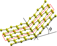
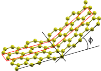
Figure 1: The structures simulated for folding around an axis along the armchair (top) and along the zig-zag direction (bottom). Unit cells are shown in red frame.

Obviously, the deformations shown in Fig. 1 are rather complex. They involve several individual torsional terms of different torsional angles and, in addition, angle-bending terms. This complicates the fitting process which is described briefly here. In order to fit an analytic form for the individual torsional term, it is necessary to separate the total torsional energy, i.e. to remove all the angle-bending contributions from the total deformation energy. This was achieved by identifying and expressing analytically, in terms of $\phi$, all the changes in bending angles induced by the folding. Then the angle-bending expressions of Eq. (3) were used to account for the individual angle-bending terms which were subsequently subtracted from the points of the total deformation energy to obtain the remaining “pure” torsional energy. More details are presented elsewhere Chatzidakis et al. .

In order to proceed with the fit, we express the total torsional energy analytically in terms of $\phi$ including all individual torsional terms that contribute. Thus, we have identified all torsional angles altered by the folding and express them in terms of $\phi$. Finally we have to assume a fitting form for the individual torsional terms, i.e. the contribution to $U_{\rm tors}$ corresponding to a single torsional angle $\omega$, and we chose the following that respects rotational symmetryJensen (2007):

$$V_{t}(\omega) = \frac{1}{2}V_{1}\left[1+\cos(\omega)\right]$$ (4)

$$+ \frac{1}{2}V_{2}\left[1-\cos(2\omega)\right]\,,$$

where $V_{1}$, $V_{2}$ are parameters to be optimized.

The fitting can be performed for several choices regarding the range of $\phi$, $[0,\phi_{\rm max}]$, and we have investigated three different ones Chatzidakis et al. . The optimal values we found are $V_{1}\sim 2\times 10^{-4}$ eV and $V_{2}\approx 0.23$ eV. Due to the small value of $V_{1}$, we can neglect the first term in Eq. (4) simplifying further the potential expression. Thus, our final proposition for the individual torsional term is

$$V_{t}(\omega)=\frac{1}{2}V_{2}\left[1-\cos(2\omega)\right],\quad V_{2}=0.23\>eV\,.$$ (5)

The fitted function reproduces reasonably well the DFT data up to folding angles of 30^∘ ($\approx$0.5 rad)Chatzidakis et al. .

III Potential Validation

The important extension provided here regarding the in-plane potential presented in Ref. Kalosakas et al., 2013 is the incorporation of the out-of-plane torsional term. This term is crucial as it permits calculations of out-of-plane deformations in planar graphenes and also simulations of non-planar sp² carbon structures, like for instance fullerenes and CNTs. In this section, the full potential that includes the in-plane terms given by Eqs. (2) and (3) and the torsional term of Eq. (5) is applied to several test cases to check whether various experimental or accurate ab initio theoretical results are reproduced. We focus on examples for which the correct description of out-of-plane deformations is important. Thus, we test our potential against (a) the energy of fullerene isomers, (b) the energy and the Young’s modulus of nanotubes with different chirality $(n,m)$, and (c) the phonon dispersion relations of graphene focusing on the out-of-plane acoustic (ZA) and optical (ZO) modes.

III.1 Fullerenes

Apart from the well known icosahedral C₆₀ fullerene Kroto et al. (1985), many other fullerenes exist. They may have different number of atoms and their pentagonal and hexagonal rings may be arranged differently Fowler and Manolopoulos (1995). A C_N fullerene is composed of 12 pentagonal and $N/2-10$ hexagonal rings, where $N$ is an even number with $N\geq 20$. Due to the different arrangement of the pentagonal and hexagonal rings in a C_N fullerene, many C_N fullerene isomers exist, the number of which rise exponentiallyFowler and Manolopoulos (1995) with $N$.

Albertazzi et alAlbertazzi et al. (1999) showed that the energy $U$ of C_N fullerene isomers rise almost linearly with the number $N_{p}$ of pentagon adjacencies. In their study they calculated the energy of the forty C₄₀ isomers using 12 different methods, from molecular mechanics to very accurate ab-initio methods. The slopes of the linear relations depend on the method used, and vary between 99.5 kJ/mol (for the ab-initio methods) to 24.4 kJ/mol (for the molecular mechanics methods). In the present study we repeat these calculations for the energy of the forty C₄₀ isomers, using our potential. In Fig. 2, we show the energy $\Delta U$ of these isomers with respect to the energy $U_{\rm graph}$ of graphene as a function of $N_{p}$, where $U_{\rm graph}=40\>U_{\rm coh}^{\rm graph}$ and $U_{\rm coh}^{\rm graph}$ is the cohesive energy of graphene. As one can see, the energy of the isomers rise linearly with the number $N_{p}$ of their pentagon adjacencies in accordance with the results of Ref. Albertazzi et al., 1999. Moreover, the energetically optimum isomer (isomer number 40:38, according to the isomer enumeration provided by Ref. Fowler and Manolopoulos, 1995) is the same as the one found by Albertazzi et al. using most of the 12 methods, including the ab-initio Albertazzi et al. (1999). Using a least squares fitting we calculate the slope $a$ and the intercept $b$ of the relation $\Delta U=aN_{p}+b$. The values we found are $a=0.42$ eV (or $a=40.5$ kJ/mol), and $b=21.4$ eV with standard error of estimate 0.53 eV. The obtained value for $a$, is within the range of slopes found by Albertazzi et al.

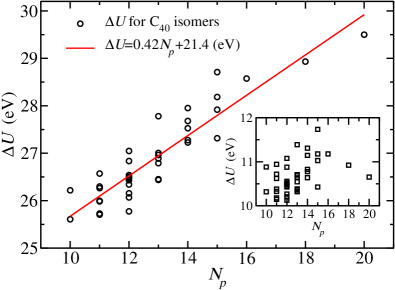
Figure 2: The energy of C₄₀ fullerene isomers, calculated with the present potential, with respect to the energy of graphene $\Delta U=U-U_{\rm graph}$ as a function of their pentagon adjacencies $N_{p}$. The inset shows the corresponding results when the out-of-plane torsional term of the potential is neglected.

Using our potential we found that the energy of the icosahedral C₆₀ fullerene with respect to the energy of graphene is $\Delta U(C_{60})=23.4$ eV or $\Delta U(C_{60})/N=0.39$ eV/atom, which is consistent with the corresponding experimentally obtained energy value $0.41\pm 0.02$ eV/atom Fthenakis (2013); Chen et al. (1991), and the theoretically obtained value 0.38 eV/atom using the DFT method at the GGA/PBE level Wirz et al. (2016). The corresponding energy found from the optimum C₄₀ isomer (isomer 40:38 of Ref. Fowler and Manolopoulos, 1995, with $N_{p}=10$) is 0.64 eV/atom, in accordance with the value 14.6 kcal/mol (0.63 eV/atom), that can be obtained from Ref. Wirz et al., 2016. In that work, the energies of both the optimum C₄₀ isomer and graphene are given with respect to that of the icosahedral C₆₀ obtained with the DFT/PBE method.

Neglecting the torsional terms of the Eq. (5), we obtain the energy $\Delta U$ of the C₄₀ fullerene isomers that is shown in the inset of Fig. 2, as a function of $N_{p}$. As one can see, the linear relation between $\Delta U$ and $N_{p}$ is not reproduced and the energy values $\Delta U$ range between 10 and 12 eV. This range is much smaller than that obtained when torsional terms are included (between 25 and 30 eV). Moreover, the energetically more favorable isomer found when torsional terms are neglected is the 40:40 isomer, with $N_{p}=12$, and not the 40:38 obtained when terms are included. As for the icosahedral C₆₀, its energy without including the torsional term, is $\Delta U(C_{60})=9.9$ eV or $\Delta U(C_{60})/N=0.17$ eV/atom, which is much smaller than the experimental value of 0.41 eV. This clearly shows the importance of the torsional terms of the proposed potential for the accurate prediction of the energetics of the fullerene structures.

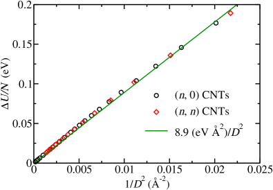
Figure 3: The energy per atom $\Delta U/N$ with respect to the energy of graphene, for the $(n,n)$ and $(n,0)$ CNTs (diamonds and circles, respectively) versus $1/D^{2}$, where $D$ is the nanotube diameter. The solid line represents a fitting with the formula $\Delta U/N=C/D^{2}$ (see text).

III.2 Carbon Nanotubes

It has been shown that the strain energy per atom $\Delta U/N=U/N-U^{graph}_{coh}$ of a CNT, i.e. the energy per atom $U/N$ with respect to the cohesive energy of graphene $U^{graph}_{coh}$, depends on its diameter $D$. Tibbetts Tibbetts (1984), using continuum elasticity theory, showed that the strain energy per atom of a CNT is given by $\Delta U/N=Ed_{0}^{3}S/(6D^{2})$, where $E$ is the Young’s modulus of the CNT, $S$ the area per atom and $d_{0}$ the interlayer separation in graphite. Assuming that $E$ and $S$ are constants, the strain energy $\Delta U/N$ has a $D^{-2}$ dependence, i.e. $\Delta U/N=C/D^{2}$, where $C$ is a constant.

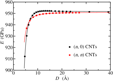
Figure 4: Young’s modulus, $E$, for the $(n,n)$ and $(n,0)$ CNTs (squares and circles, respectively) as a function of their diameter $D$. Points show numerical results and solid lines fittings with analytical relations (see text).

The fitting value of $C$ varies, depending on the method used for the energy calculations. Using the Tersoff Tersoff (1988) potential, Sawada and Hamada Sawada and Hamada (1992) found $C=5.64$ eV Ų, while TersoffTersoff (1992) estimated $C=5.36$ eV Ų. Zhong-can et al. Zhong-can et al. (1997) using continuum elasticity found $C=6.12$ eV Ų. Based on tight binding calculations, Xin et al. Xin et al. (2000) found $C=5.76$ eV Ų, Molina et al. Molina et al. (1996) estimated $C=5.64$ eV Ų, while Hernandez et al. Hernández et al. (1999) found $C=8.7$ eV Ų for the $(n,0)$ CNTs, and $C=8.1$ eV Ų for the $(n,n)$ CNTs. Using a tight binding density functional method, Adams et al. Adams et al. (1992) calculated $C=8.46$ and 8.37 eV Ų for the $(n,n)$ and the $(n,0)$ CNTs respectively. Sánchez-Portal et al. Sánchez-Portal et al. (1999), performing DFT calculations in the LDA levelSánchez-Portal et al. (1997); Soler et al. (2002), found $C=8.00$ eV Ų for the $(n,n)$, while for the (8,4) and (10,0) CNTs they found slightly larger values, $C=8.60$ and 8.64 eV Å², respectively.

In Fig. 3, we show (with points) the energy $\Delta U/N$ as a function of $1/D^{2}$ of various optimized $(n,n)$ and $(n,0)$ CNTs, for $D>6$ Å, using the model potential presented here. As we can see, there is an almost linear relation between $\Delta U/N$ and $1/D^{2}$, in agreement with all the previous studies. Fitting a linear function of $1/D^{2}$ to these energy values, we find that both $(n,0)$ and $(n,n)$ CNTs can be approximately described by $\Delta U/N=C/D^{2}$, where $C=$8.9 eV Å². This fitting is shown by continuous line in Fig. 3. The obtained value of $C$, using the force field presented here, is close to the tight binding values of Hernandez et al Hernández et al. (1999), the tight binding density functional values of Adams et al Adams et al. (1992) and the DFT/LDA values of Sánchez-Portal et al Sánchez-Portal et al. (1999). This value is consistent to the results obtained with the more accurate methods, in contrary to the corresponding results of other, less accurate atomistic models.

Note a very small discrepancy between this analytical relation and the numerical data for intermediate values of $D$ in Fig. 3, revealing that a $1/D^{2}$ dependence of the energy is not so precise. A more accurate relation for the energy per atom $\Delta U/N$ should include an additional term depending on $1/D^{4}$, as reported by Kanamitsu and Saito Kanamitsu and Saito (2002). Including this term in our fitting, we find $\Delta U/N=9.68(\mbox{eV \AA}^{2})/D^{2}-45.3(\mbox{eV \AA}^{4})/D^{4}$.

Furthermore, we calculate the Young’s modulus $E$ of the $(n,0)$ and $(n,n)$ CNTs using the potential proposed here, through the relation

$$E=\frac{1}{2}\frac{\partial^{2}U}{\partial x^{2}}\frac{l}{\pi rd_{0}},$$ (6)

where $U$ represents the deformation energy of a CNT segment with length $l$ deformed by $x$ ($x\equiv\delta l$), $r$ is the CNT radius and $d_{0}=3.34$ Å  is the width of the nanotube wall, where we have adopted the convention that the width $d_{0}$ of the nanotube is the same as the interlayer separation of graphite. In Fig. 4, we plot the calculated $E$ values against the CNT diameter $D$. As one can see, our model predicts a rapid increase of the Young’s modulus $E$ of CNTs as a function of their diameter $D$, for diameters up to 8 Å. For larger diameters, as the strain due to rolling drops, $E$ remains almost constant with a value equal to that of graphene. This result is in accordance with earlier studies using other model potentials Meo and Rossi (2006); Chang and Gao (2003); Popov et al. (2000), as well as tight binding Goze et al. (1999) and ab-initio calculations Hernández et al. (1999). Moreover, we fit a quadratic function of $1/D^{2}$ to these data. The fitting functions for $(n,0)$ and $(n,n)$ CNTs are $E=950+175/D^{2}-23500/D^{4}$ and $E=950-175/D^{2}-7080/D^{4}$, respectively, where $E$ is given in GPa and $D$ in Å. These analytical relations are also shown in Fig. 4 with lines and we see that these functions perfectly fit to the calculated $E$ values. It is worth noting that the corresponding Young’s modulus value predicted for graphene using our model potential is $E\approx 950$ GPa.

III.3 Phonon dispersion relations of graphene

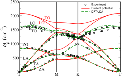
Figure 5: Phonon dispersion relation of graphene along the $\Gamma$MK$\Gamma$ path calculated using the potential presented here and the DFT method at the LDA level, compared with experimental data (points) of the phonon dispersion of graphiteMohr et al. (2007); Maultzsch et al. (2004).

As another test of the force field presented here, we calculate the phonon dispersion relation of graphene along the $\Gamma$MK$\Gamma$ path and compare it with experimental values Mohr et al. (2007); Maultzsch et al. (2004) as well as DFT calculations. The phonon dispersion relations were obtained using a hand-made computer code which calculates the Hessian matrix as the derivative of the atomic forces by inducing small perturbations of the atomic positions.

DFT phonon calculations were performed at the LDA level employing the Perdue and ZungerPerdew and Zunger (1981) exchange and correlation functional using the SIESTA code Sánchez-Portal et al. (1997); Soler et al. (2002). We also used norm-conserving Trullier and Martins pseudopotenitalsTroullier and Martins (1991), and 10$\times$10$\times$1 Monkhorst Pack k-point grid. As for the basis set, we used a double-$\zeta$ polarized basis set of atomic orbitals with a 100 Ry energy cut-off. For the phonon band structure calculations we used the “vibra” utility of SIESTA.

The phonon dispersion calculated with our potential and DFT are shown in Fig. 5 together with the experimental data. For comparison with known, widely used atomistic potentials, we show in Fig. 6, the dispersion obtained using our potential together with that using the Tersoff Tersoff (1988, 1989), a reparameterized Tersoff (Tersoff-2010) Lindsay and Broido (2010), and LCBOP Los and Fasolino (2003) potentials, in panels (a) - (c), respectively. In order to quantify the performance of different schemes in phonon dispersion calculations, we show in Table 1 the RMSD error (root of the mean squared deviation with respect to experimental values) for all calculation schemes shown in Figs. 5 and 6. The numerical data for the dispersions obtained by the Tersoff, Tersoff-2010, and LCBOP potentials are taken from Ref. Koukaras et al., 2015. As seen in Figs. 5, 6 and Table 1, in general, DFT reproduces more accurately phonon dispersions than any of the considered classical atomistic potentials, as expected, despite the fact that the simple LDA approximation was used. However, LO branch is an exception for which LCBOP and Tersoff-2010 seem to perform better.

Table 1: The RMSD error (in cm^-1) of the phonon dispersion of graphene for each phonon mode separately (first to sixth row) calculated with the present force field, Tersoff, Tersoff-2010, and LCBOP atomistic potentials, as well as using DFT. The error is calculated with respect to the experimental points of the phonon dispersion of graphiteMohr et al. (2007); Maultzsch et al. (2004). We also include the RMSD error for (i) the overall data of all modes (seventh row), (ii) all but excluding LO and TO modes (eighth row), (iii) the out-of-plane ZA and ZO modes (ninth row), and (iv) all phonons with low frequencies $\omega_{p}<1000$ cm^-1 (tenth row).

	Present potential	Tersoff (α)	Tersoff-2010 (α)	LCBOP (α)	DFT/LDA
ZA	25.7	71.5	38.8	99.9	18.6
ZO	49.4	37.5	238.8	97.8	26.6
LA	97.1	137.6	21.3	32.4	21.2
LO	273.7	773.1	36.1	32.8	130.4
TA	86.2	325.5	80.2	26.0	18.0
TO	446.0	479.7	294.7	264.3	46.7
All modes	235.7	472.2	149.8	118.1	72.9
All modes, excluding LO and TO	75.3	192.4	121.2	67.1	21.2
Out-of-plane modes: ZA and ZO	40.1	56.0	176.4	98.8	23.2
Small frequencies ($<\mbox{10}^{3}\mbox{ cm}^{-1}$)	55.5	191.4	132.8	71.9	19.5
(α) RMSD values are taken from Ref. Koukaras et al., 2015.

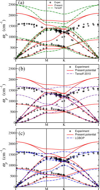
Figure 6: Phonon dispersion relation of graphene along the $\Gamma$MK$\Gamma$ path calculated using the potential presented here compared with (a) the Tersoff, (b) the Tersoff-2010, and (c) the LCBOP potentials. The experimental points of the phonon dispersion of graphiteMohr et al. (2007); Maultzsch et al. (2004) are also included.

Clearly the present potential, despite its simplicity, is quite accurate in reproducing the phonon dispersion for all modes in the regime of small frequencies. Its performance in the linear regime of the LA and TA acoustic modes is excellent and in very close agreement with the experimental and the DFT results. This is demonstrated in Table 1 where we show the RMSD errors only for those phonons that their experimental frequency is smaller than 1000 cm^-1 (see last row). As we see, in this regime, only the DFT results are superior to the present potential, while those of the other atomistic potentials, including the two recent ones, are less accurate. The only exception from the good performance in this regime is the upper part of the TA mode, where the results of the present potential seem to deviate from the experimental data.

Regarding the ZO and ZA modes (the lower optical and acoustic modes, respectively), representing the out-of-plane phonons in graphene, the performance of the present potential is quite satisfactory, and substantially better than any of the other atomistic potentials we discuss here. This is quantified in Table 1, where we include the RMSD errors for these modes (see ninth row). Thus, in conclusion, the out-of-plane terms introduced in the present work, augmenting the in-plane terms introduced in Ref. Kalosakas et al., 2013, add to the potential the capability to calculate very accurately the out-of-plane phonon modes ZA and ZO of graphene.

Overall, the potential presented here is superior than the Tersoff potential. This is the case for almost all modes as shown in Table 1 except ZO, for which, although our potential is very accurate, Tersoff potential performs surprisingly well. Compared to the two more recent potentials, i.e. Tersoff-2010 and LCBOP, the present potential shows a worse overall agreement with experiment. However, the overall performance of the present potential is negatively affected mainly by its inability to reproduce the LO and TO modes and, to a lesser extend, the high frequency regimes of TA mode. These phonon frequencies are substantially overestimated. Its failure, however, is less dramatic than Tersoff’s potential. We mention that these modes are rather unaffected by the out-of-plain torsional terms introduced in the present work. Instead, they depend strongly on the in-plane bond-stretching and angle-bending terms. A possible future improvement would be to extend the present model by including more distant stretching interactions (than just first neighbors) or introducing mixed stretching-bending terms. Such terms can also be fitted to ab-initio data similarly to the terms already included in the present potential.

It should be stressed that graphene possesses anomalous optical-phonon dispersion at the $\Gamma$ and K points since alterations of the electronic screening occurs for the atomic vibration at these particular pointsPiscanec et al. (2004); Ferrari (2007) There exist Kohn anomalies at these points reducing the frequency of the LO branch by tens or hundreds cm^-1. Our model does not take into account such effects.

Note that there exist graphene properties, like the lattice thermal conductivity at room temperature, that seem to entirely determined by the lower frequency and the out-of-plane phonon modes Wei et al. (2014); Gu and Yang (2015). In particular, it has been found that even for higher temperatures, up to 800-1000 $K$, the contribution of the high frequency LO and TO modes in the thermal conductivity does not exceed a value of around 5% Wei et al. (2014); Gu and Yang (2015). Our proposed potential may combine improved efficiency and accuracy for studying such properties of graphene using atomistic simulations.

IV Conclusions

In conclusion, we introduced a torsional term for sp² carbon systems in order to complement the in-plane force field which was presented previously Kalosakas et al. (2013). For this task, we performed DFT calculations for two different, appropriately chosen, graphene-nanoribbon structures that were folded around their middle line. The torsional terms were fitted to reproduce the deformation energy of these structures as a function of the folding angle. The proposed torsional potential has the simple form of Eq. (5).Our aim was to keep the proposed force field as simple as possible, targeting computational efficiency, for large scale simulations. Indeed, in a test simulation with LAMMPS, our force field was found to be 3 and 4 times faster than Tersoff/Tersoff-2010 and LCBOP potentials, respectively.

The full proposed potential was tested in several characteristic cases. More specifically, we demonstrated that, with the inclusion of torsional terms, the linear dependence of the energy of C₄₀ fullerene isomers on the number of adjacent pentagons is obtained, while the energy of the more favorable C₆₀ and C₄₀ fullerenes is accurately reproduced. Then, we showed that, in the case of carbon nanotubes, the proposed potential reproduces the $1/D^{2}$ dependence of the strain energy on the nanotube diameter $D$, while its predictions for the Young’s moduli of nanotubes as a function of their diameter are in accordance with existing calculations.

Finally, we calculated the phonon dispersion of graphene and compared with other atomistic force fields and DFT, as well as to experimental data. The performance of the present potential for the phonon modes can be separated in two frequency regions. For the high frequency phonons ($\omega_{p}>1000$ cm^-1), especially for LO, TO modes, our potential overestimates phonon frequencies substantially, however, it is still better than Tersoff potential. In the low frequency regime, $\omega_{p}<1000$ cm^-1 (including the behavior of acoustic modes close to the $\Gamma$ point), its accuracy is quite satisfactory with results closer to the experimental data and the DFT values as compared to other widely used atomistic potentials. We stress the success of the present potential in reproducing the ZA and ZO out-of-plane phonon modes of graphene very accurately, and in better agreement with experiment compared to other recent and popular classical force fields. This close agreement is a result of the out-of-plane torsional terms introduced in the present work.

Acknowledgements: We acknowledge helpful discussions with E. N. Koukaras and A. P. Sgouros. We also thank A. P. Sgouros for performing the efficiency comparison of the presented potential in LAMMPS. The research leading to the present results has received funding from Thales project “GRAPHENECOMP”, co-financed by the European Union (ESF) and the Greek Ministry of Education (through ESPA program). NNL acknowledges support from the Hellenic Ministry of Education/GSRT (ESPA), through “Advanced Materials and Devices” program (MIS:5002409) and EU H2020 ETN project “Enabling Excellence” Grant Agreement 642742. The FORTH/ ICE-HT contributors acknowledges the support of the European Research Council Advanced Grant “Tailor Graphene” (no. 321124, 2013-2018).

References

- Kroto et al. (1985) H. W. Kroto, J. R. Heath, S. C. O’Brien, R. F. Curl, and R. E. Smalley, Nature 318, 162 (1985).
- Iijima (1991) S. Iijima, Nature 354, 56 (1991).
- Novoselov et al. (2004) K. S. Novoselov, A. K. Geim, S. V. Morozov, D. Jiang, Y. Zhang, S. V. Dubonos, I. V. Grigorieva, and A. A. Firsov, Science 306, 666 (2004).
- Castro Neto et al. (2009) A. H. Castro Neto, F. Guinea, N. M. R. Peres, K. S. Novoselov, and A. K. Geim, Rev. Mod. Phys. 81, 109 (2009).
- Ferrari (2007) A. C. Ferrari, Solid State Commun. 143, 47 (2007).
- Ferrari et al. (2015) A. C. Ferrari, F. Bonaccorso, V. Fal’ko, K. S. Novoselov, S. Roche, P. Boggild, S. Borini, F. H. L. Koppens, V. Palermo, N. Pugno, et al., Nanoscale 7, 4598 (2015).
- Zhu et al. (2010) Y. Zhu, S. Murali, W. Cai, X. Li, J. W. Suk, J. R. Potts, and R. S. Ruoff, Advanced Materials 22, 3906 (2010).
- Geim and Grigorieva (2013) A. K. Geim and I. V. Grigorieva, Nature 499, 419 (2013).
- Bhimanapati et al. (2015) G. R. Bhimanapati, Z. Lin, V. Meunier, Y. Jung, J. Cha, S. Das, D. Xiao, Y. Son, M. S. Strano, V. R. Cooper, et al., ACS Nano 9, 11509 (2015).
- Tersoff (1988) J. Tersoff, Phys. Rev. Lett. 61, 2879 (1988).
- Tersoff (1989) J. Tersoff, Phys. Rev. B 39, 5566 (1989).
- Lindsay and Broido (2010) L. Lindsay and D. A. Broido, Phys. Rev. B 81, 205441 (2010).
- Brenner (1990) D. W. Brenner, Phys. Rev. B 42, 9458 (1990).
- Senftle et al. (2016) T. P. Senftle, S. Hong, M. M. Islam, S. B. Kylasa, Y. Zheng, Y. K. Shin, C. Junkermeier, R. Engel-Herbert, M. J. Janik, H. M. Aktulga, et al., npj Computational Materials 2, 15011 (2016).
- Srinivasan et al. (2015) S. G. Srinivasan, A. C. T. van Duin, and P. Ganesh, J. Phys. Chem. A 119, 571 (2015).
- Los and Fasolino (2003) J. H. Los and A. Fasolino, Phys. Rev. B 68, 024107 (2003).
- Los et al. (2005) J. H. Los, L. M. Ghiringhelli, E. J. Meijer, and A. Fasolino, Phys. Rev. B 72, 214102 (2005).
- Stuart et al. (2000) S. J. Stuart, A. B. Tutein, and J. A. Harrison, J. Chem. Phys. 112, 6472 (2000).
- Wei et al. (2011) D. Wei, Y. Song, and F. Wang, J. Chem. Phys. 134, 184704 (2011).
- Fasolino et al. (2007) A. Fasolino, J. H. Los, and M. I. Katsnelson, Nature Mater. 6, 858 (2007).
- Zakharchenko et al. (2009) K. V. Zakharchenko, M. I. Katsnelson, and A. Fasolino, Phys. Rev. Lett. 102, 046808 (2009).
- Zhao et al. (2009) H. Zhao, K. Min, and N. R. Aluru, Nano Lett. 9, 3012 (2009).
- Xu and Buehler (2010) Z. Xu and M. J. Buehler, ACS Nano 4, 3869 (2010).
- Neek-Amal and Peeters (2010) M. Neek-Amal and F. M. Peeters, Appl. Phys. Lett. 97, 153118 (2010).
- Sgouros et al. (2014) A. Sgouros, M. M. Sigalas, K. Papagelis, and G. Kalosakas, J. Phys.: Condens. Matter 26, 125301 (2014).
- Fthenakis and Tománek (2012) Z. G. Fthenakis and D. Tománek, Phys. Rev. B 86, 125418 (2012).
- Zhang et al. (2014) P. Zhang, L. Ma, F. Fan, Z. Zeng, C. Peng, P. E. Loya, Z. Liu, Y. Gong, J. Zhang, X. Zhang, et al., Nature Communications 5, 3782 (2014).
- Fthenakis and Lathiotakis (2015) Z. G. Fthenakis and N. N. Lathiotakis, Phys. Chem. Chem. Phys. 17, 16418 (2015).
- Yoon et al. (2016) K. Yoon, A. Rahnamoun, J. L. Swett, V. Iberi, D. A. Cullen, I. V. Vlassiouk, A. Belianinov, S. Jesse, X. Sang, O. S. Ovchinnikova, et al., ACS Nano 10, 8376 (2016).
- Sgouros et al. (2016) A. P. Sgouros, G. Kalosakas, C. Galiotis, and K. Papagelis, 2D Materials 3, 025033 (2016).
- Meng et al. (2017) F. Meng, C. Chen, and J. Song, Carbon 116, 33 (2017).
- Jain et al. (2017) S. K. Jain, V. Juriĉić, and G. T. Barkema, 2D Materials 4, 015018 (2017).
- Kalosakas et al. (2013) G. Kalosakas, N. N. Lathiotakis, C. Galiotis, and K. Papagelis, J. Appl. Phys. 113, 134307 (2013).
- Plimpton (1995) S. Plimpton, Journal of Computational Physics 117, 1 (1995), URL http://www.sciencedirect.com/science/article/pii/S002199918571039X.
- (35) Lammps molecular dynamics simulator, http://lammps.sandia.gov/index.html.
- (36) G. D. Chatzidakis, G. Kalosakas, Z. G. Fthenakis, and N. N. Lathiotakis, (2017, in print); ArXiv e-prints, 2017, arXiv:1707.09059.
- Perdew et al. (1996) J. P. Perdew, K. Burke, and M. Ernzerhof, Phys. Rev. Lett. 77, 3865 (1996).
- Giannozzi et al. (2009) P. Giannozzi, S. Baroni, N. Bonini, M. Calandra, R. Car, C. Cavazzoni, D. Ceresoli, G. L. Chiarotti, M. Cococcioni, I. Dabo, et al., J. Phys.: Condens. Matter 21, 395502 (19pp) (2009).
- (39) A. Dal Corso, http://www.quantum-espresso.org/wp-content/uploads/upf_files/C.pbe-rrkjus.UPF, c.pbe-rrkjus.upf.
- Jensen (2007) F. Jensen, Introduction to Computational Chemistry (John Wiley & Sons, Ltd, 2007), 2nd ed., ISBN 978-0-470-01187-4.
- Fowler and Manolopoulos (1995) P. W. Fowler and D. E. Manolopoulos, An atlas of fullerenes (Clarendon Press, Oxford, 1995).
- Albertazzi et al. (1999) E. Albertazzi, C. Domene, P. W. Fowler, T. Heine, G. Seifert, C. Van Alsenoy, and F. Zerbetto, Phys. Chem. Chem. Phys. 1, 2913 (1999).
- Fthenakis (2013) Z. G. Fthenakis, Mol. Phys. 111, 3289 (2013).
- Chen et al. (1991) H. S. Chen, A. R. Kortan, R. C. Haddon, M. L. Kaplan, C. H. Chen, A. M. Mujsce, H. Chou, and D. A. Fleming, Appl. Phys. Lett. 59, 2956 (1991).
- Wirz et al. (2016) L. N. Wirz, R. Tonner, A. Hermann, R. Sure, and P. Schwerdtfeger, Journal of Computational Chemistry 37, 10 (2016).
- Tibbetts (1984) G. G. Tibbetts, J. Cryst. Growth 66, 632 (1984).
- Sawada and Hamada (1992) S. Sawada and N. Hamada, Solid State Commun. 83, 917 (1992).
- Tersoff (1992) J. Tersoff, Phys. Rev. B 46, 15546 (1992).
- Zhong-can et al. (1997) O.-Y. Zhong-can, Z.-B. Su, and C.-L. Wang, Phys. Rev. Lett. 78, 4055 (1997).
- Xin et al. (2000) Z. Xin, Z. Jianjun, and O.-Y. Zhong-can, Phys. Rev. B 62, 13692 (2000).
- Molina et al. (1996) J. M. Molina, S. S. Savinsky, and N. V. Khokhriakov, J. Chem. Phys. 104, 4652 (1996).
- Hernández et al. (1999) E. Hernández, C. Goze, P. Bernier, and A. Rubio, Appl. Phys. A 68, 287 (1999).
- Adams et al. (1992) G. B. Adams, O. F. Sankey, J. B. Page, M. O’Keeffe, and D. A. Drabold, Science 256, 1792 (1992).
- Sánchez-Portal et al. (1999) D. Sánchez-Portal, E. Artacho, J. M. Soler, A. Rubio, and P. Ordejón, Phys. Rev. B 59, 12678 (1999).
- Sánchez-Portal et al. (1997) D. Sánchez-Portal, P. Ordejón, E. Artacho, and J. M. Soler, Int. J. Quant. Chem. 65, 453 (1997).
- Soler et al. (2002) J. M. Soler, E. Artacho, J. D. Gale, A. García, J. Junquera, P. Ordejón, and D. Sánchez-Portal, J. Phys.: Condens. Matter 14, 2745 (2002).
- Kanamitsu and Saito (2002) K. Kanamitsu and S. Saito, J. Phys. Soc. Japan 71, 483 (2002).
- Meo and Rossi (2006) M. Meo and M. Rossi, Composites Science and Technology 66, 1597 (2006).
- Chang and Gao (2003) T. Chang and H. Gao, J. Mech. Phys. Solids 51, 1059 (2003).
- Popov et al. (2000) V. N. Popov, V. E. Van Doren, and M. Balkanski, Phys. Rev. B 61, 3078 (2000).
- Goze et al. (1999) C. Goze, L. Vaccarini, L. Henrard, P. Bernier, E. Hemandez, and A. Rubio, Synthetic Metals 103, 2500 (1999).
- Mohr et al. (2007) M. Mohr, J. Maultzsch, E. Dobardžić, S. Reich, I. Milošević, M. Damnjanović, A. Bosak, M. Krisch, and C. Thomsen, Phys. Rev. B 76, 035439 (2007).
- Maultzsch et al. (2004) J. Maultzsch, S. Reich, C. Thomsen, H. Requardt, and P. Ordejón, Phys. Rev. Lett. 92, 075501 (2004).
- Perdew and Zunger (1981) J. P. Perdew and A. Zunger, Phys. Rev. B 23, 5048 (1981).
- Troullier and Martins (1991) N. Troullier and J. L. Martins, Phys. Rev. B 43, 1993 (1991), URL https://link.aps.org/doi/10.1103/PhysRevB.43.1993.
- Koukaras et al. (2015) E. N. Koukaras, G. Kalosakas, C. Galiotis, and K. Papagelis, Sci. Rep. 5, 12923 (2015).
- Piscanec et al. (2004) S. Piscanec, M. Lazzeri, F. Mauri, A. C. Ferrari, and J. Robertson, Phys. Rev. Lett. 93, 185503 (2004).
- Wei et al. (2014) Z. Wei, J. Yang, K. Bi, and Y. Chen, J. Appl. Phys. 116, 153503 (2014).
- Gu and Yang (2015) X. Gu and R. Yang, J. Appl. Phys. 117, 025102 (2015).