Efficient Inferencing of Compressed Deep Neural Networks

Abstract

Large number of weights in deep neural networks makes the models difficult to be deployed in low memory environments such as, mobile phones, IOT edge devices as well as “inferencing as a service” environments on cloud. Prior work has considered reduction in the size of the models, through compression techniques like pruning, quantization, Huffman encoding etc. However, efficient inferencing using the compressed models has received little attention, specially with the Huffman encoding in place. In this paper, we propose efficient parallel algorithms for inferencing of single image and batches, under various memory constraints. Our experimental results show that our approach of using variable batch size for inferencing achieves 15-25% performance improvement in the inference throughput for AlexNet, while maintaining memory and latency constraints.

I Introduction

Deep neural networks have been used extensively over the last decade in applications ranging from computer vision [21] to speech recognition [14] and natural language processing [9]. In this paper, we focus particularly on convolutional neural networks (CNNs) which have become ubiquitous in object recognition, image classification, and retrieval. Almost all of the recent successful recognition systems are built on top of this architecture (see [20, 11, 13, 30]). A simple convolution neural network consists of a sequence of layers, with every layer of the network transforming one volume of activations to another through a differentiable function. Thus for an image classification problem, the input image is transformed layer by layer from the original pixel values to the final class scores.

Convolution networks comprise of different types of layers including convolution (CONV), fully connected layer (FC), pooling layer (POOL), Rectified Linear Unit (ReLU) etc. Of these, the CONV and the FC layers contain weights and biases, which are parameters trainable over some data set. Thus the CONV/FC layers perform transformations that are functions of not only the activations in the input volume, but also of the parameters of the respective layers (the weights and biases of the neurons). On the other hand, the RELU/POOL layers implement fixed functions.

As datasets increase in size, so do the number of layers in the CNNs and the number of parameters, in order to absorb the enormous amount of supervision. In 1998 Lecun et al. designed a CNN model LeNet-5 with less than 1M parameters to classify handwritten digits [22], while in 2012, Krizhevsky et al. [21] won the ImageNet competition with 60M parameters and 8 layers (this correspond to the popular AlexNet network). Deepface classified human faces with 120M parameters [29], and Coates et al. [8] scaled up a network to 10B parameters. Karen Simonyan and Andrew Zisserman  [28] developed VGG-16 network with 16 layers and 138M parameters.

The large number of weights in powerful and complex neural networks makes the models difficult to be deployed in low memory environments such as, mobile phones, IOT edge devices etc. Large networks do not fit in on-chip storage and are stored in external DRAM: thus they need to be fetched every time for the inferencing of each test sample. This leads to multiple issues. Firstly, the inference time shoots up due to the overhead of external memory accesses. Secondly, fetching the model from the external DRAM consumes large amount of energy. For instance, Han et al. [16] states that the energy cost per fetch ranges from 5pJ for 32bit coefficients in on-chip SRAM to 640pJ for 32bit coefficients in off-chip LPDDR2 DRAM: thus running a 1 billion connection neural network, at 20Hz would require 12.8W just for DRAM access - this prohibits inferencing on a typical mobile device. A similar issue arises for “inferencing as a service” environment on the cloud: in this case the networks need to be loaded before the inferencing, thus increasing memory requirement and cost. It is therefore advisable to have the model reside permanently in the memory. Moreover many applications like visual recognition require multiple models for inferencing: thus it is feasible to have all the models loaded apriori in memory only if the models are pretty small in size.

To address the above issues, significant work has been done to reduce the size of the networks. The objective in the ideal scenario is to generate a model of smaller size, with limited loss of accuracy in the prediction, and no sacrifice in the inference time. Model compression can be effected through a combination of pruning, weight sharing and encoding of the connection weights. In the pruning step, the network is pruned by removing the redundant connections of the network. Next, the weights are quantized so that multiple connections share the same weight, thus only the codebook (effective weights) and the indices need to be stored. The codebook is generally of small size, and hence the indices can be represented with fewer bits than that required for the original weights. Finally, some encoding (like Huffman coding) is performed to take advantage of the biased distribution of effective weights in further reducing the model size.

Neural network pruning has been pioneered even in the early development of neural networks (see  [27]), and has been implemented through various strategies over the years. Anwar et al. [6] and Molchanov et al.  [25] employ structured pruning at the level of feature maps and kernels. The advantage of this scheme of pruning is that the resultant connection matrix can be considered dense. However their strategy is more suited for convolution layers. Song Han et al. [16] have considered the weight based pruning where they remove all connections whose weights are lower than fixed threshold. Their pruning strategy (along with quantization and Huffman encoding) was able to get the model size of AlexNet reduced from 240MB to 6.9MB, and that of VGG-16 from 552MB to 11.3MB, without loss of accuracy on Imagenet dataset. A lot of literature is available for weight sharing and quantisation as well. Half-precision networks (Amodei et al.,  [5]) cut sizes of neural networks in half. XNOR-Net (Rastegari et al.,  [26]), DoReFa-Net (Zhou et al.,  [31]) and network binarization (Courbariaux et al. [10]; Lin et al. [24]) use aggressively quantized weights, activations and gradients to further reduce computation during training, however, the extreme compression rate comes with a loss of accuracy. Hubara et al. [18] and Li Liu [23] propose ternary weight networks to trade off between model size and accuracy. Zhu et al. [32] propose trained ternary quantization which uses two full-precision scaling coefficients for each layer, where these coefficients are trainable parameters. Gong. et al. [12] consider vector quantization methods for compressing the parameters of CNNs. HashedNets [7] uses hash function to randomly group connection weights into hash buckets, so that all connections within the same hash bucket share a single parameter value.

In this work, we consider the compression strategy as suggested by Han et al. (see  [16, 17]). As stated before, their compression technique has gained significant popularity due to the very little loss in accuracy for a number of networks and datasets. Since all connections with weights below a threshold are removed from the network, the pruned network becomes a sparse structure that is stored using compressed sparse row (CSR) or compressed sparse column (CSC) format. The model is further compressed by storing the index difference instead of the absolute position, and encoding this difference in $k$ bits for each layer: for an index difference larger than $2^{k}$, zero padding is employed. Finally Huffman encoding is employed on both the weight clusters and the index differences to ensure that more common cluster centres and index differences are represented with fewer bits.

The real challenge with compressed models lies in processing them for inferencing. Efficient inferencing using the compressed models has received little attention. As stated before, with pruning the matrix becomes sparse and the indices are stored in the form of relative differences. With weight sharing, a short (8-bit) index for each weight is stored. More indirection is added with Huffman encoding. All of these increase the complexity of the inferencing process, making it inefficient on CPUs and GPUs. The trivial method of uncompressing the matrix back to dense form and performing the inferencing in a standard framework (like Caffe, Tensorflow etc) is not a good choice because of the excessive memory usage and the running time. Previous work has considered hardware and software accelerators to facilitate computation on compressed models. Han et al. [15] has proposed EIE, an efficient inference engine, that performs customized sparse matrix vector multiplication and handles weight sharing with no loss of efficiency. However this requires specialized hardware to be designed to act as the accelerator. On the software side, Intel Math Kernel Library (MKL [2]) provides optimized sparse solvers for matrix-matrix and matrix-vector multiplications. However it does not incorporate relative indexing and Huffman encoding, which are necessary to gain the desired compression levels. Tensorflow has recently incorporated Gemmlowp library (see  [1]) for fast inferencing using eight-bit arithmetic rather than floating-point - however, this does not handle pruned and encoded models.

Another important aspect is the transition of mobile devices to multi-core CPUs. The current generation of mobile processors are being designed to deal with the increased number of high performance use cases. To satisfy the rapidly growing demand for performance and form factor sleekness, the industry has begun to adopt Symmetrical Multiprocessing even on mobile systems. This calls for leveraging multiple cores to facilitate faster inferencing even in low memory systems. Nvidia has studied and developed GPU-Based Inferencing (see [4]); in a recent work Huynh et al. [19] has proposed DeepMon, a mobile GPU based deep learning inference system for mobile devices. However all of these work on uncompressed models. Thus very little has been studied on parallel domain for compressed (in particular encoded) models.

Another key factor is the batch size that should be used for inferencing on these limited resource systems. It is well-known that larger batch size for inferencing increase both the throughput (since computing resources can be utilized more efficiently) and the latency. Thus inferencing applications strive to maximize a usable batch size while keeping latency under a given threshold. The maximum batch size is also determined by the amount of the available memory in the system. However, this varies dynamically depending on the system load. Hence the batch size for achieving the maximum throughput can only be figured out at the time of inferencing.

The focus of this paper is to study and propose optimizations for efficient inferencing compressed models under various resource limitations. Our main contributions are as follows:

• We propose a framework for inferencing of images with compressed models that rely on pruning, quantization, relative indexing and encoding techniques for compression. To the best of our knowledge, this is the first effort towards efficient inferencing using compressed models under memory constraints.

• We propose parallel algorithms under this framework that can use tuned math libraries available on the platform to perform efficient inferencing. Our framework uses different blocking schemes to optimize the inferencing time, wherein the best choice of the block size depends on the layer of the network, its sparsity and the batch size used.

• We show that variable size batching that performs inferencing on a different number of activations in each layer can lead to better inferencing performance. To this effect, we develop a novel dynamic programming based algorithm to figure out the optimal batch size to be used in the inferencing for each individual layer under memory and latency constraints.

• Our experimental results show that our approach of using variable batch size for inferencing achieves 15-25% performance improvement in the inference throughput for AlexNet, while maintaining memory and latency constraints.

The rest of the paper is organized as follows. In Section II, we motivate our problem by defining the challenges and the use cases. Section III establishes necessary preliminaries and concepts before we present our inferencing schemes in Section IV. Our results for different blocking schemes are presented in Section V. We next study variable size batching for inferencing in Section V-C, the results of which are presented in Section VI. Finally, we conclude in Section VII.

II Discussion on use cases and challenges

Today, a large number of Artificial Intelligence (AI) applications rely on using deep learning models for various tasks, such as, image classification, speech recognition, natural language understanding, natural language generation and so on. Due to the significant improvement in performance achieved by the deep learning models, there is a natural trend to use these models on the applications running on mobile phone and other edge devices in the context of IOT (Internet of Things). For example, more and more people now want to take pictures using their mobile phones and get information on the building and surroundings around them in a foreign place. Usage of voice based assistants on mobile phones and other home devices is another increasing trend. Applications in the area of augmented reality involves continuous image recognition with results being reported on a VR display to provide more information regarding the environment to the individual. For example, in security, this can be used for identity detection. Similarly, in self-driven cars, deep learning models are used to inference in real-time using data collected from a combination of sensing technologies including visual sensors, such as cameras, and range-to-object detecting sensors, such as lasers and radar. Increased instrumentation in various industries such as agriculture, manufacturing, renewable energy and retail generates lot structured and unstructured data which preferably needs to be analyzed at the edge device and so that real-time action can be taken.

For the scenarios described above, inferencing can be done either on the cloud (or server) or on the edge device itself. However, offloading inferencing to the cloud can be impractical in lot of situations due to wireless energy overheads, turn-around latencies and data security reasons. On the other hand, given the sheer size of the deep learning models, inferencing on mobile/edge devices poses other kind of challenges on resources, such as memory, compute and energy which need to be utilized efficiently while continuing to provide high accuracy and similar latency.

Even when inferencing is done on the cloud, resources have to be efficiently utilized to keep the cost of inferencing minimum for the cloud vendor as the cost of inferencing is directly dependent on resource utilization. Just as an example, a vendor providing ”Inferencing as a service” for image classification may want to keep hundreds of deep learning models customized for various domains and users in memory in order to provide the low response time. This calls for storing compressed models in-memory and directly inferencing using the compressed model when the requests come in. All of this has to be done without compromising on the latency and accuracy of the inferencing.

III Preliminaries

III-A Inferencing as matrix computations

A fully-connected (FC) layer of a deep neural network (DNN) performs the computation as

$$b=Wa+v.$$ (1)

where $a$ and $b$ are respectively the input activation vector and the output activation vector, $v$ is the bias, $W$ is the weight matrix. The output activations of Equation  1 is computed element-wise as:

$$b_{i}=\sum_{j=0}^{n-1}W_{ij}a_{j}+v_{i}.$$ (2)

For a typical FC layer like FC7 of VGG-16 or AlexNet, the activation vectors are 4K long, and the weight matrix is 4K x 4K (16M weights). Weights are represented as single-precision floating-point numbers so such a layer requires 64MB of storage. Similarly for FC6 layer of AlexNet the weight matrix is of dimension 4096 x 9216, for FC6 layer of VGG-16 the weight matrix is of dimension 4096 x 25088.

The computation of a convolution (CONV) layer of a CNN can also be expressed as a matrix-matrix multiplication operation. The input activation for the CONV layer is a 3-dimensional tensor. The convolution layer’s parameters consist of a set of learnable filters (or kernels), which have a local connectivity along width and height in the input, but extend through the full depth of the input volume. Each filter is convolved across the width and height of the input volume, computing the dot product between the entries of the filter with the input and producing a 2-dimensional activation map of that filter. Stacking the activation maps for all filters along the depth dimension forms the full output volume of the convolution layer. The dot products between the filters and local regions of the input, can be formulated as a matrix-matrix multiplication, by flattening out the local regions of the input to individual columns and the layer weights to rows: the result of a convolution is now equivalent to performing one large matrix which evaluates the dot product between every filter and every receptive field location. See [3] for details.

III-B Representation of compressed model

As stated before, this paper considers the compression technique, as suggested by Han et al. [16, 17] to reduce the size of the DNNs without loss of accuracy, obtained through a combination of pruning, weight sharing and Huffman encoding. Pruning makes weight matrix $W$ sparse: the pruned matrix $W$ is stored in a variant of the standard compressed row storage (CSR) format. The standard CSR representation works as follows: instead of storing the entire matrix $W$ of dimension $r$ x $c$, vectors, one of floating-point numbers (val), and the other two of integers ($col\_ind$, $row\_ptr$) are used. The $val$ vector stores the values of the nonzero elements of $W$, as they are traversed in a row-wise fashion. The $row\_ptr$ vector stores the locations in the $val$ vector that start a row, that is, if $val(m)=W_{ij}$ then $row\_ptr(i)\leq m<row\_ptr(i+1)$. By convention, we define $row\_ptr(r+1)=nnz+1$, where $nnz$ is the number of nonzeros in $W$. The $col\_ind$ vector is used to store the column indexes of the elements in the val vector. Figure 1b shows the CSR representation for the matrix given in Figure 1a.

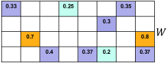
(a) Sparse Matrix.

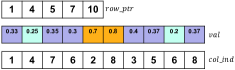
(b) CSR Format.

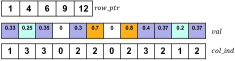
(c) Relative Column Index.

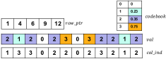
(d) Quantized Weight.

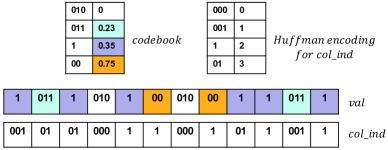
(e) Huffman Encoded Model.

Figure 1: Representation of a compressed model.

The $col\_ind$ vector can be further compressed by making each of its entries exactly $k$ bits. This is achieved by modifying $col\_ind$ as follows: if $val(i)$ is the first non-zero entry of any particular row, then $col\_ind(i)$ is set to the corresponding column number; else $col\_ind(i)$ is set to the number of columns between the current non-zero and the last non-zero entry of the row. If more than $2^{k}$ zeros appear before a non-zero entry, we add a zero in both the $val$ and the $col\_ind$ vectors. This representation format is the CSR with relative column index. Figure 1c shows the relative indexed CSR of Figure 1b with $k=2$. Since the first non-zero column of second row exceeds 4, we pad a zero at the fourth location of both $val$ and $col\_ind$. Further compression is effected using quantization where similar valued non-zero entries of $val$ are clustered together to share the same value. If $r$ bits are used for quantization, we use at most ($2^{r}-1$) distinct non-zero values along with 0 in quantized values, and each entry of the $val$ vector is a $r$ bit index to the corresponding cluster centre. The cluster centre values are stored in the codebook. Figure 1d shows the quantized model representation (quantization here is done using $2$ bits), entries denoted by the same colour in the matrix of Figure 1a are mapped to a single cluster, and each entry of the $val$ vector is a $2$ bit index to the corresponding cluster centre. The codebook is also shown. Finally Figure 1e shows the Huffman encoded bit representations of $val$ and $col\_ind$ vectors. Clearly, entry $i$ of the $row\_ptr$ array will a 2-tuple, the first field storing the starting address for row $i$ in $val$, while the second stores the starting address for row $i$ in $col\_ind$.

IV Inferencing using Compressed Models

In this section, we discuss the various approaches for inferencing using the compressed model, where the compressed model is stored in the format as shown in the previous section. Clearly, the trivial method of exploding the model back to the dense format and doing the computation (using standard frameworks like Caffe, Tensorflow etc) is not a good choice since the entire purpose of model compression gets defeated because of the excessive memory usage. The other extreme of decoding element by element of the matrix and doing the operations on the decoded element has little memory overhead, but is computationally inefficient. This calls for the need to develop an efficient stand-alone module (independent of the Caffe/Tensorflow framework) for inferencing using the compressed model. The naïve algorithm for doing the inferencing is presented in Algorithm 1. The idea here is to work sequentially on the individual rows of the weight matrix (line 3). For a particular row, the $col\_ind$ and the $val$ entries for that row are first Huffman-decoded (line 5-6); this is followed by converting relative column index of $col\_ind$ to absolute index (line 7) and creating an $abs\_val$ array which is essentially the $val$ array with its entries replaced by the corresponding codebook entires. All these steps in fact create the arrays in Figure 1a from Figure 1e for a particular row segment. Finally we call MKL routine $mkl\_scsrmm$ for sparse matrix-matrix multiplication of $abs\_val(i)$ and $a$ to compute $b[i,:]$.

1:  Input: $row\_ptr$ array, entry $i$ of which is a tuple of starting address of row $i$ in $val$ and that in $col\_ind$. $val$ Huffman encoded cluster index bit stream. $col\_ind$ Huffman encoded rel. indexed column bit stream. ${\cal C}$ codebook of quantized weights. $a$ input activation matrix. 2:  Output: $b$ output activation matrix. 3:  for every entry $i$ of the $row\_ptr$ array do 4:     Set $val\_begin(i)$, $val\_end(i)$, $col\_begin(i)$, $col\_end(i)$ for row $i$ as follows   $\langle val\_begin(i),col\_begin(i)\rangle\leftarrow row\_ptr(i)$   $\langle val\_end(i),col\_end(i)\rangle\leftarrow row\_ptr(i+1)$. 5:     $dec\_val(i)$ $\leftarrow$ Huffman decoding of bit stream in $val$ between $val\_begin(i)$ and $val\_end(i)$. 6:     $dec\_col(i)$ $\leftarrow$ Huffman decoding of bit stream in $col\_ind$ between $col\_begin(i)$ and $col\_end(i)$. 7:     $abs\_col(i)$ $\leftarrow$ Prefix sum of $dec\_col(i)$. 8:     Set $abs\_val(i)[j]$ $\leftarrow$ ${\cal C}[dec\_val(i)[j]]$ , $\forall j$. 9:     $b[i,:]$ += MKL_CSRMM($abs\_val(i)$, $a$) 10:  end for

Algorithm 1 Naïve algorithm for inferencing using compressed model

The above algorithm can be parallelized by employing different threads to operate on different rows of the weight matrix. Moreover MKL internally can use multiple threads for sparse matrix operations. However Algorithm 1 faces multiple drawbacks. Firstly, the algorithm decodes an entire row of the matrix, and thus the memory requirement becomes significant for large matrices. Secondly, most algorithms for matrix multiplication work more efficiently using blocks rather than individual elements, to achieve necessary reuse of data in local memory. The advantage of this approach is that the small blocks can be moved into the fast local memory and their elements can then be repeatedly used. This motivates us to employ blocking even for compressed model inferencing, which we describe next.

IV-A Blocking of Weight Matrix

The general idea of blocking is to organize the data structures in a program into chunks called blocks. The program is structured so that it loads a block into the L1 cache, does all the reads and writes that it needs to on that block, then discards the block, loads in the next block, and so on. Similar to standard matrix multiplication, the blocking algorithm for inferencing shall work by partitioning the matrices into submatrices and then exploiting the mathematical fact that these submatrices can be manipulated just like scalars. Instead of storing the original weight matrix in row major format, we need to ensure that any particular block of the matrix is stored in contiguous memory. This will make certain that the Huffman decoding happens on contiguous memory locations and generates the submatrix corresponding to a block.

See Figure 2a and Figure 2b for illustration. Suppose the original weight matrix stored in dense row major format is of dimension 8x8, and we decide to work on blocks each sized 4x4. We first convert this matrix to 4 x 16 format, such that each row of the new matrix stores elements of the corresponding block of the old matrix in contiguous locations. This new matrix is then stored in CSR format with relative indexing and Huffman encoding, as discussed in the previous section.
Size of the modified model:

It is observed that the non zeroes in the weight matrix are uniformly distributed, thus the size of the $val$ and $col\_ind$ vectors does not change a lot (even with zero padding in the compressed format) when the matrix is stored in block contiguous fashion. The number of rows in the modified matrix is same as the number of blocks in the original matrix, and may be larger or smaller than that in the original matrix depending on the block size. From experimental results, it is however observed, that change in model size due to this difference in the size of the $row\_ptr$ is insignificant. Hence we can assume that storing the model in block contiguous fashion does not add to memory overhead.

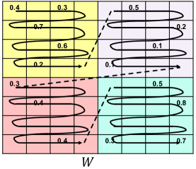
(a) Original Connection Matrix.

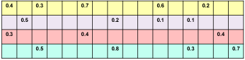
(b) Modified Connection Matrix

Figure 2: Representation of a compressed model.

IV-B Blocked Inferencing Procedure

Next we present our inferencing algorithm using the blocked storage scheme. Our algorithm ensures that once a row of the connection matrix (which corresponds to a block in the original weight matrix) is decoded, the decoded entries are used for all the computations that require them. This is illustrated in Figure 3. A row is decoded and multiplied with all possible subblocks of input activation matrix to generate partial results for the output activation matrix. The blocked inferencing algorithm is presented in Algorithm 2.

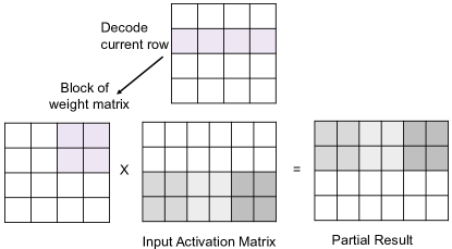
Figure 3: Blocked inference scheme.

1:  Input: Compressed model stored in $bh$ x $bw$ block contiguous manner with $row\_ptr$ array, entry $i$ of which is a tuple $\langle x,y\rangle$ where $x$ and $y$ being respectively starting address of row $i$ in $val$ and that in $col\_ind$. $val$ Huffman encoded cluster index bit stream. $col\_ind$ Huffman encoded relative indexed column bit stream. ${\cal C}$ codebook of quantized weights. $a$ input activation matrix with $a_{rows}$ rows 2:  Output: $b$ output activation matrix 3:  for every entry $i$ of the $row\_ptr$ array do 4:     Set $val\_begin(i)$, $val\_end(i)$, $col\_begin(i)$, $col\_end(i)$ for row $i$ as follows   $\langle val\_begin(i),col\_begin(i)\rangle\leftarrow row\_ptr(i)$   $\langle val\_end(i),col\_end(i)\rangle\leftarrow row\_ptr(i+1)$. 5:     $dec\_val(i)$ $\leftarrow$ Huffman decoding of bit stream in $val$ between $val\_begin(i)$ and $val\_end(i)$. 6:     $dec\_col(i)$ $\leftarrow$ Huffman decoding of bit stream in $col\_ind$ between $col\_begin(i)$ and $col\_end(i)$. 7:     $abs\_col(i)$ $\leftarrow$ Prefix sum of $dec\_col(i)$. 8:     Set $abs\_val(i)[j]$ $\leftarrow$ ${\cal C}[dec\_val(i)[j]]$ , $\forall j$. 9:     Arrange $abs\_val(i)$ as $bh$ x $bw$ block. 10:     col_id = $(i\%(a_{rows}/bw))*bw$ 11:     row_id = $(i/(a_{rows}/bw))*bh$ 12:     b[row_id:(row_id+bh-1),:] += MKL_CSRMM($abs\_val(i)$, a[col_id:(col_id+bw-1),:] ) 13:  end for

Algorithm 2 Algorithm for block inferencing

V Experimental Results with Blocking

In this section, we present the experimental results for our block inferencing procedure. We begin by specifying the system configurations and the dataset.

V-A System and Dataset

For running our experiments (also the ones in Section VI), we have used Intel Xeon CPU E5-2697 system. It has two NUMA nodes with 12 cores, each with frequency of 2.70GHZ. The system has 32KB, 256KB and 30MB of L1, L2 and L3 cache respectively. We consider compressed models for two popular deep neural networks, AlexNet and VGG-16. For each of these models we consider the compressed configurations corresponding to four different pruning percentages. The first configuration corresponds to the procedure applied in [16]. Table Ia and Table Ib present the pruning percentages of all the layers in this configuration. We refer to this configuration as conventional in subsequent discussion. The compressed model sizes of AlexNet and VGG-16 for this configuration are respectively 6.81 MB and 10.64 MB. The other three configurations correspond respectively to 70%, 80% and 90% pruning of all the layers of the network. We consider these configurations to study how our scheme performs for a wide range of sparsity spectrum of the compressed models. 8 bit (5 bit) quantization for CONV (FC) layers and 4 bit (5 bit) relative indexing for AlexNet (VGG-16) is employed for all the configurations.

Layer	Pruning %
conv1	16
conv2	62
conv3	65
conv4	63
conv5	37
fc6	91
fc7	91
fc8	75

(a) AlexNet

Layer	Pruning %
conv1_1	42
conv1_2	78
conv2_1	66
conv2_2	64
conv3_1	47
conv3_2	76
conv3_3	58
conv4_1	68
conv4_2	73
conv4_3	66
conv5_1	65
conv5_2	71
conv5_3	64
fc6	96
fc7	96
fc8	77

(b) VGG-16

TABLE I: Compressed AlexNet and VGG-16 models.

V-B Blocking results

Our first set of experiments is aimed to study the effect of variation of block sizes on the inference time (both the decoding time and the computation time) for individual layers corresponding to the different configurations of the compressed models. Figure 4a and  4b show the decoding time, computation time and total time, with different block sizes for FC6 layer of AlexNet and VGGnet, using batch size of 16. The models used for these runs correspond to the conventional configuration. All these experiments employ MKL with 4 threads for computation.

We observe that for very small block sizes, the decoding and the computation time are pretty high due to overhead of the too many function calls. For very large block sizes, the level of parallelism gets limited, leading to increase in the inference time. Figure 4c and  4d show the same charts with batch size of 256. We note that for smaller batch size, the total time is dominated by the decoding time, whereas the computation time takes over at larger batch sizes. However the nature of variation of inference time with the block size is consistent across batch sizes. We observe similar nature of plots for other configurations and batch sizes as well.

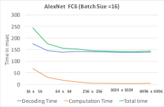
(a) AlexNet Batch size16

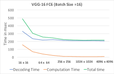
(b) VGG-16 Batch size 16

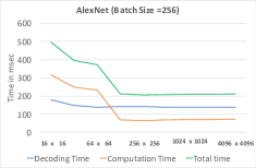
(c) AlexNet Batch size 256

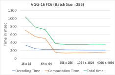
(d) VGG-16 Batch size 256

Figure 4: Inference Time Variation with Block Size.

We also note that the working memory increases with increase in block size. Table II presents the working memory required for matrix matrix multiplication for FC6 layer of AlexNet and VGG-16. Since there is not significant difference in the inference timings between block sizes in range 128 x 128 to 1024 x 1024, we fix 128 x 128 as our block size for the subsequent experiments.

Blocksize	AlexNet	VGG-16
16 x 16	1.26KB	0.92KB
32 x 32	4.57KB	3.42KB
64 x 64	17.33KB	12.97KB
128 x 128	67.40KB	50.22KB
256 x 256	265.78KB	197.26KB
512 x 512	1.03MB	781.52KB
1024 x 1024	4.11MB	2.98MB
2048 x 2048	14.76MB	11.42MB
4096 x 4096	36.88MB	42.38MB

TABLE II: Working Memory Requirement for FC6 layer

We next observe the variation of activation memory requirement and the inference time with batch sizes. Table III presents the results for batch sizes of 16 and 256. Clearly, for a fixed batch size, the activation memory required by the convolution layers is more than that of the fully-connected layers. Inferencing applications on a low resource system generally come with a cap on the available memory. Suppose we consider a fictitious scenario where the maximum available memory is 20MB. From Table III, it makes sense to run the fully connected layers with batch size 256, since the memory required is well below the permissible threshold, and there is significant increase in throughput if we process in batch of 256. For the convolution layers, however, processing in batch of 256 is not a desirable option because of the large memory overhead. This motivates us to use different batch sizes for different layers during the inferencing. We present this in more detail in the next section.

	Memory (MB)		Time (ms)
Layer	batch-size	batchsize	batchsize	batchsize
	16	256	16	256
conv1	17.72	283.59	349.93	5408.93
norm1	17.72	283.59	98.87	1597.83
pool1	4.27	68.34	11.68	176.42
conv2	11.39	182.25	341.72	5745.49
norm2	11.39	182.25	68.06	1081.80
pool2	2.64	42.25	7.12	116.49
conv3	3.96	63.38	153.11	2573.47
conv4	3.96	63.38	204.01	3135.62
conv5	2.64	42.25	135.66	2242.94
pool5	0.56	9.00	1.92	25.72
fc6	0.25	4.00	51.77	112.62
fc7	0.25	4.00	21.06	46.61
fc8	0.06	0.98	9.66	22.61

TABLE III: Memory Requirement and Inference time for AlexNet individual layers

V-C Inferencing with Variable Batch Size

It is clear from the results shown in the previous section that using a larger batch for inferencing increases the throughput as computing resources are utilized more efficiently. However, an issue with inferencing larger batches is the increase in inferencing latency (due to wait time while assembling a batch, and because larger batches take longer to process). Moreover the memory requirement for the input and the output activations and buffer memory also increases for larger batch size. Thus applications work with large batch sizes while keeping the latency and memory utilization within certain thresholds. The problem becomes more challenging since the available memory varies dynamically depending on the system load; hence the batch size for achieving the maximum throughput can be figured out only at the time of inferencing. Moreover, the memory requirement and the computation time for inferencing varies with the layers even for a fixed batch size. Thus it might be advantageous to do the inferencing using different batch sizes for different layers. We address this issue by proposing a dynamic programming based algorithm for determining variable batch sizes for different layers for efficient inferencing. We describe our dynamic program below.

V-D Dynamic Programming

Let $L_{1}$, $L_{2}$, $\cdots$, $L_{f}$ denote the layers of the DNN. For $i$ = 1, 2, $\cdots$, $f$, let Time$(i,B)$ denote the time required to perform the inferencing computations for layer $L_{i}$ of the DNN using a batch size of $B$. Next, we let IN$(i,B)$ and OUT$(i,B)$ respectively denote the input activation and output activation memory required to perform inferencing of layer $L_{i}$ with a batch size of $B$. Further, let WS$(i)$ denote the size of the temporary workspace required for layer $L_{i}$ computations (for instance this includes the buffer memory required to decode blocks of the connection matrix for $L_{i}$). All the values IN$(i,B)$, OUT$(i,B)$, WS$(i)$ and Time$(i,B)$ are obtained once for a given compressed model. Note that the total memory required to perform inferencing computations for layer $L_{i}$ with a batch size of $B$ is captured by

$${\rm IN}(i,B)+{\rm WS}(i)+{\rm OUT}(i,B).$$

Let TOT denote the total memory available for performing the inference computations for the entire model.

We now describe the dynamic program to determine the optimal batch size to be used at all the individual layers in order to maximize the overall throughput of the inferencing. For this we define a configuration: a configuration is a tuple $\langle i,B,A\rangle$, where $i$ denotes the layer $L_{i}$, $B$ denotes a batch size and $A$ denotes amount of memory. We maintain a dynamic program table OPT. An entry OPT$(i,B,A)$ of the dynamic program denotes the minimum time to perform the inferencing computations for layers $L_{1}$-$L_{i}$, when a batch size of $B$ is used for layer $L_{i}$, and $A$ units of memory (out of TOT) are not available for performing the inferencing computations for layers $L_{1}$-$L_{i}$ (this memory is reserved for performing inferencing computations from layer $L_{i+1}$ to layer $L_{f}$). Thus, we only have available (TOT - $A$) units of memory for inference computations of layers $L_{1}$ to $L_{i}$.

We say that configuration $\langle i,B,A\rangle$ is feasible if the total memory required for performing inferencing computations at layer $L_{i}$ with a batch size of $B$ is within the available memory bound, i.e.,

$$A+{\rm IN}(i,B)+{\rm WS}(i)+{\rm OUT}(i,B)\leq{\rm TOT}.$$

We now describe the recurrence relation for computing the entries of the dynamic programming table OPT$(\cdot,\cdot,\cdot)$. For simplicity, we assume that for every $i$, the batch size used for inferencing computations at layer $L_{i-1}$ is no more than the batch size used for the inferencing computations at layer $L_{i}$. Clearly, OPT$(i,B,A)$ can be finite only if $\langle i,B,A\rangle$ is feasible. Suppose that layer $L_{i}$ is computed with batch size $B$ and layer $L_{i-1}$ with a batch size $b$. For simplicity, we consider all $b\leq B$ such that $b$ divides $B$. For a given $b$, the inferencing computations for layer $L_{i-1}$ will be performed in $(B/b)$ phases, wherein in each phase a batch of size $b$ will be processed up to layer $L_{i-1}$. After the end of these phases, the $B$ output activations of layer $L_{i-1}$ will be fed as input activations to layer $L_{i}$. Note that before the processing of the last of these phases, IN$(i,B-b)$ amount of output activation need to be buffered. Thus the total memory available for processing up to layer $L_{i-1}$ gets reduced by IN$(i,B-b)$ as this is required for storing the activations before processing layer $L_{i}$.

We are now ready to present the recurrence relation. For any $i>1$,

$$\begin{split}{\rm OPT}(i,&B,A)={\rm Time}(i,B)\quad\quad+\\ &\quad\min\limits_{b\leq B}\left\{(B/b)*{\rm OPT}(i-1,b,A+{\rm IN}(i,B-b))\right\}\\ &\quad\mbox{subject to}\quad\quad\text{ $\langle i,B,A\rangle$ is feasible}\end{split}$$

For the base case i.e., for $i$ = 1.

$${\rm OPT}(1,B,A)=\begin{cases}{\rm Time}(1,B),&\text{if $\langle 1,B,A\rangle$ is feasible}.\\ \infty,&\text{otherwise}.\end{cases}$$

The maximum throughput for the inferencing is obtained by considering the configuration that yields the minimum inference time per input which is

$$\min\limits_{B}\frac{{\rm OPT}(f,B,0)}{B}.$$

The above dynamic program can be easily extended to ensure that the latency of inferencing is always less than some specified threshold. In the recurrence relation, if OPT$(i,B,A)$ exceeds the threshold value for some $i$, $B$, and $A$, we make OPT$(i,B,A)$ $\leftarrow$ $\infty$. This makes sure that our optimal solution never has larger latency.

V-E Additional Storage and Computation Overhead

The table OPT$(\cdot,\cdot,\cdot)$ needs to be evaluated for each entry in order to figure out the individual layer batch sizes that maximise the overall throughput. We now figure out the additional storage and computation that is needed for the dynamic programming space complexity for standard networks like AlexNet. The total number of layers in AlexNet is 14. For requested input count of 64, we consider batch sizes in range 1 to 64 for the second dimension. For the case where the additional available memory is twice of the model size, the third dimension is considered from 0 to 14MB in steps of 100KB. Thus the total size of the table is around 500KB. Each entry computation of the table computes the minimum over a set of possible batch sizes. Thus the computation complexity is at most $\cal B$ times the size of the table, where $\cal B$ is the maximum number of distinct batch sizes considered.

We begin our inferencing with a pre-processing step, which computes the individual layer batch sizes that maximise the overall throughput using the above dynamic program. The actual inferencing uses the batch sizes outputted from the dynamic program.

VI Experimental Results with Batch Size

In this section, we validate the results of our dynamic programming algorithm on practical test cases with AlexNet model. Suppose the user requests for inference of a set of $K$ images, and is interested to get the maximum throughput for the inference. We consider the scenarios where the total memory in the system (in addition to the model) is 1.5x, 2x and 2.5x times the model size. Our baseline is selecting a fixed batch size such that (i) running any layer of inferencing using that batch size does not violate the memory constraints (ii) out of all possible batch sizes which satisfy (i), the baseline returns the batch size with maximum throughput. We compare this baseline from our dynamic programming output, which uses variable batch sizes for different layers. We perform our experiments $K=32,64,128$ and with all the four configurations of AlexNet model (conventional pruning and 70%, 80%, 90% pruning). Figure 5a -  5c compares the results of our dynamic program algorithm with the baseline (fixed batch size) output for AlexNet with conventional pruning. The x-axis shows the additional memory available (w.r.t to the model size) over the model, and the y-axis plots the total time to infer K images. Our results show that the dynamic programming approach improves the throughput by 15-25% over the fixed batch size approach.

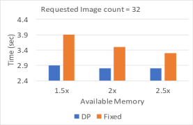
(a) K=32

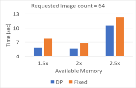
(b) K=64

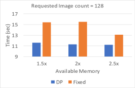
(c) K=128

Figure 5: Fixed batch size (baseline) time vs Time outputted from Dynamic Programming for AlexNet with conventional pruning.

Layer	1.5x	2x	2.5x
conv1	2	4	6
norm1	4	4	6
pool1	4	4	6
conv2	4	4	6
norm2	4	4	6
pool2	4	4	6
conv3	4	4	6
conv4	4	4	6
conv5	4	4	6
pool5	4	4	32
fc6	64	64	60
fc7	64	64	60
fc8	64	64	60

TABLE IV: Variable batching for AlexNet.

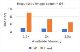
(a) Pruning = 70%

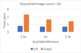
(b) Pruning = 80%

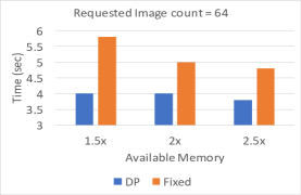
(c) Pruning = 90%

Figure 6: Fixed batch size (baseline) time vs Time outputted from Dynamic Programming for AlexNet with 70%, 80% and 90% pruning.

Table IV shows the dynamic programming output corresponding to the above run for K = 64. It is observed that the optimal inferencing scheme uses smaller batch sizes for the convolution layers (because of the larger memory overhead), and combines intermediate outputs to perform fully connected layer operations with larger batch sizes. This matches our intuition which motivated us to develop the dynamic programming based solution. The dynamic programming solution corresponding to column 2.5x picks 60 as the batchsize for final layers: thus for this case, we again compute the solution for requested input of 4, and report the total time for inferencing. The baseline corresponding to these runs use fixed batch size of 3, 5 and 7 for additional memory of 1.5x, 2x and 2.5x respectively.

Figure 6a -  6c extends our results to the other configurations of the AlexNet model, namely, the 70%, 80% and 90% pruned models. We show these results for fixed K of 64. Our results show that the dynamic programming approach performs well over the fixed batch size approach for these scenarios as well.

VII Concluding Remarks and Future work

In this paper, we study efficient inferencing using compressed models under memory constraints. We propose parallel algorithms that can use tuned math libraries available on the platform to perform inferencing efficiently with compressed models that rely on pruning, quantization, relative indexing and encoding techniques for compression. We study different blocking schemes and study the effect of block sizes on the layer of the network, its sparsity and the batch size used for AlexNet and VGG-16. We observe that in a typical neural network inference, different layers have different sized activation memory required; thus it is beneficial to use variable sized batching across different layers. We propose a novel dynamic programming based algorithm that figures out the optimal batch size for throughput maximization for the case where the batch size used for inferencing in individual layers is a monotonically increasing sequence, i.e., where larger batch sizes can be used for layers closer to the output. We show that our dynamic programming solution achieves 15-25% performance improvement in the inference throughput over the solution employing fixed batch size across layers. A future work in this direction is to relax the assumption of monotonically increasing batch sizes. Our results are applicable in training of neural network models as well. There has been recent effort for employing compressed models in reducing training time: our techniques, e.g dynamic batching, will be useful here for designing a faster forward phase.

References

- [1] How to quantize neural networks with tensorflow. https://www.tensorflow.org/performance/quantization.
- [2] Intel math kernel library. https://software.intel.com/en-us/mkl.
- [3] Why gemm is at the heart of deep learning. https://petewarden.com/2015/04/20/why-gemm-is-at-the-heart-of-deep-learning/.
- [4] Gpu-based deep learning inference: A performance and power analysis. https://www.nvidia.com/content/tegra/embedded-systems/pdf/jetson_tx1_whitepaper.pdf, 2015.
- [5] Dario Amodei, Rishita Anubhai, Eric Battenberg, Carl Case, Jared Casper, Bryan Catanzaro, Jingdong Chen, Mike Chrzanowski, Adam Coates, Greg Diamos, Erich Elsen, Jesse Engel, Linxi Fan, Christopher Fougner, Tony Han, Awni Y. Hannun, Billy Jun, Patrick LeGresley, Libby Lin, Sharan Narang, Andrew Y. Ng, Sherjil Ozair, Ryan Prenger, Jonathan Raiman, Sanjeev Satheesh, David Seetapun, Shubho Sengupta, Yi Wang, Zhiqian Wang, Chong Wang, Bo Xiao, Dani Yogatama, Jun Zhan, and Zhenyao Zhu. Deep speech 2: End-to-end speech recognition in english and mandarin. CoRR, abs/1512.02595, 2015.
- [6] Sajid Anwar, Kyuyeon Hwang, and Wonyong Sung. Structured pruning of deep convolutional neural networks. JETC, 13(3):32:1–32:18, 2017.
- [7] Wenlin Chen, James T. Wilson, Stephen Tyree, Kilian Q. Weinberger, and Yixin Chen. Compressing neural networks with the hashing trick. In Proceedings of the 32nd International Conference on Machine Learning, ICML 2015, Lille, France, 6-11 July 2015, pages 2285–2294, 2015.
- [8] Adam Coates, Brody Huval, Tao Wang, David J. Wu, Bryan Catanzaro, and Andrew Y. Ng. Deep learning with COTS HPC systems. In Proceedings of the 30th International Conference on Machine Learning, ICML 2013, Atlanta, GA, USA, 16-21 June 2013, pages 1337–1345, 2013.
- [9] Ronan Collobert, Jason Weston, Léon Bottou, Michael Karlen, Koray Kavukcuoglu, and Pavel Kuksa. Natural language processing (almost) from scratch. J. Mach. Learn. Res., 12:2493–2537, November 2011.
- [10] Matthieu Courbariaux and Yoshua Bengio. Binarynet: Training deep neural networks with weights and activations constrained to +1 or -1. CoRR, abs/1602.02830, 2016.
- [11] Jeff Donahue, Yangqing Jia, Oriol Vinyals, Judy Hoffman, Ning Zhang, Eric Tzeng, and Trevor Darrell. Decaf: A deep convolutional activation feature for generic visual recognition. In Proceedings of the 31th International Conference on Machine Learning, ICML 2014, Beijing, China, 21-26 June 2014, pages 647–655, 2014.
- [12] Yunchao Gong, Liu Liu, Ming Yang, and Lubomir D. Bourdev. Compressing deep convolutional networks using vector quantization. CoRR, abs/1412.6115, 2014.
- [13] Yunchao Gong, Liwei Wang, Ruiqi Guo, and Svetlana Lazebnik. Multi-scale orderless pooling of deep convolutional activation features. In Computer Vision - ECCV 2014 - 13th European Conference, Zurich, Switzerland, September 6-12, 2014, Proceedings, Part VII, pages 392–407, 2014.
- [14] Alex Graves and Jürgen Schmidhuber. Framewise phoneme classification with bidirectional LSTM and other neural network architectures. Neural Networks, 18(5-6):602–610, 2005.
- [15] Song Han, Xingyu Liu, Huizi Mao, Jing Pu, Ardavan Pedram, Mark A. Horowitz, and William J. Dally. EIE: efficient inference engine on compressed deep neural network. In 43rd ACM/IEEE Annual International Symposium on Computer Architecture, ISCA 2016, Seoul, South Korea, June 18-22, 2016, pages 243–254, 2016.
- [16] Song Han, Huizi Mao, and William J. Dally. Deep compression: Compressing deep neural network with pruning, trained quantization and huffman coding. CoRR, abs/1510.00149, 2015.
- [17] Song Han, Jeff Pool, John Tran, and William J. Dally. Learning both weights and connections for efficient neural networks. CoRR, abs/1506.02626, 2015.
- [18] Itay Hubara, Matthieu Courbariaux, Daniel Soudry, Ran El-Yaniv, and Yoshua Bengio. Quantized neural networks: Training neural networks with low precision weights and activations. CoRR, abs/1609.07061, 2016.
- [19] Loc N. Huynh, Youngki Lee, and Rajesh Krishna Balan. Deepmon: Mobile gpu-based deep learning framework for continuous vision applications. In Proceedings of the 15th Annual International Conference on Mobile Systems, Applications, and Services, MobiSys ’17, pages 82–95, 2017.
- [20] Yangqing Jia, Evan Shelhamer, Jeff Donahue, Sergey Karayev, Jonathan Long, Ross B. Girshick, Sergio Guadarrama, and Trevor Darrell. Caffe: Convolutional architecture for fast feature embedding. In Proceedings of the ACM International Conference on Multimedia, MM ’14, Orlando, FL, USA, November 03 - 07, 2014, pages 675–678, 2014.
- [21] Alex Krizhevsky, Ilya Sutskever, and Geoffrey E. Hinton. Imagenet classification with deep convolutional neural networks. In Proceedings of the 25th International Conference on Neural Information Processing Systems - Volume 1, NIPS’12, pages 1097–1105, 2012.
- [22] Yann Lecun, Léon Bottou, Yoshua Bengio, and Patrick Haffner. Gradient-based learning applied to document recognition. In Proceedings of the IEEE, pages 2278–2324, 1998.
- [23] Fengfu Li and Bin Liu. Ternary weight networks. CoRR, abs/1605.04711, 2016.
- [24] Zhouhan Lin, Matthieu Courbariaux, Roland Memisevic, and Yoshua Bengio. Neural networks with few multiplications. CoRR, abs/1510.03009, 2015.
- [25] Pavlo Molchanov, Stephen Tyree, Tero Karras, Timo Aila, and Jan Kautz. Pruning convolutional neural networks for resource efficient transfer learning. CoRR, abs/1611.06440, 2016.
- [26] Mohammad Rastegari, Vicente Ordonez, Joseph Redmon, and Ali Farhadi. Xnor-net: Imagenet classification using binary convolutional neural networks. In Computer Vision - ECCV 2016 - 14th European Conference, Amsterdam, The Netherlands, October 11-14, 2016, Proceedings, Part IV, pages 525–542, 2016.
- [27] Russell Reed. Pruning algorithms-a survey. Trans. Neur. Netw., 4(5):740–747, September 1993.
- [28] Karen Simonyan and Andrew Zisserman. Very deep convolutional networks for large-scale image recognition. CoRR, abs/1409.1556, 2014.
- [29] Yaniv Taigman, Ming Yang, Marc’Aurelio Ranzato, and Lior Wolf. Deepface: Closing the gap to human-level performance in face verification. In 2014 IEEE Conference on Computer Vision and Pattern Recognition, CVPR 2014, Columbus, OH, USA, June 23-28, 2014, pages 1701–1708, 2014.
- [30] Matthew D. Zeiler and Rob Fergus. Visualizing and understanding convolutional networks. In Computer Vision - ECCV 2014 - 13th European Conference, Zurich, Switzerland, September 6-12, 2014, Proceedings, Part I, pages 818–833, 2014.
- [31] Shuchang Zhou, Zekun Ni, Xinyu Zhou, He Wen, Yuxin Wu, and Yuheng Zou. Dorefa-net: Training low bitwidth convolutional neural networks with low bitwidth gradients. CoRR, abs/1606.06160, 2016.
- [32] Chenzhuo Zhu, Song Han, Huizi Mao, and William J. Dally. Trained ternary quantization. CoRR, abs/1612.01064, 2016.