Hong-Ou-Mandel Interference

Abstract

This article is a detailed introduction to Hong-Ou-Mandel (HOM) interference, in which two photons interfere on a beamsplitter in a way that depends on the photons’ distinguishability. We begin by considering distinguishability in the polarization degree of freedom. We then consider spectral distinguishability, and show explicitly how to calculate the HOM dip for three interesting cases: 1) photons with arbitrary spectral distributions, 2) spectrally entangled photons, and 3) spectrally mixed photons.

1 Introduction

When two indistinguishable photons interfere on a beam splitter, they behave in an interesting way. This effect is known as Hong-Ou-Mandel (HOM) interference, named after Chung Ki Hong, Zhe Yu Ou and Leonard Mandel, who experimentally verified the effect in 1987 [1]. HOM interference shows up in many places, both in fundamental studies of quantum mechanics and in practical implementations of quantum technologies. At its heart, HOM interference is quite simple to understand. But it can also be very rich once different aspects of the incoming light are considered.

This document contains a step-by-step account of how these more interesting effects can be modelled. We begin, in Section 2, with a basic model of two photons interfering on a beam splitter. We then consider the photons’ polarization degree of freedom in Section 3, and show that the output state (after the beam splitter) is fundamentally different depending on the photons’ relative polarizations. We then extend the model to account for the photons’ spectro-temporal properties in Section 4, and show how to calculate the famous HOM dip. As concrete examples, we examine three interesting cases: 1) photons with arbitrary spectral distributions, 2) spectrally entangled photons, and 3) spectrally mixed photons.

This document is intended to serve as a pedagogical guide; we therefore go into much more detail than in a typical research paper.

2 A basic model of two-photon interference

Consider two photons incident on a beam splitter, as shown in Figure 1. The combined two-photon state before arriving at the beam splitter, i.e. the input state, is:

$$|\psi_{\textrm{in}}\rangle_{ab}={} \hat{a}^{\dagger}_{j}\hat{b}^{\dagger}_{k}|0\rangle_{ab}=|1;j\rangle_{a}|1;k\rangle_{b}\,,$$ (1)

where $\hat{a}^{\dagger}_{j}$ and $\hat{b}^{\dagger}_{k}$ are bosonic creation operators in beam splitter modes, $a$ and $b$, respectively. In addition to being identified by their respective beam splitter modes, the photons can have other properties, labeled by $j$ and $k$, that determine how distinguishable they are.

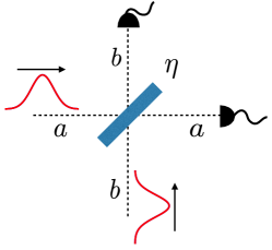
Figure 1: Two photons interfere on a beam splitter of reflectivity $\eta$. Upon exiting the beam splitter, the photons are detected.

Some examples of such additional properties are the photon’s polarization, spectral mode [2, 3], temporal mode [4], arrival time, or transverse spatial mode [5]. For the time being, we make no assumptions about the photons’ level of distinguishability.

The evolution of a state as it interferes on a beam splitter with reflectivity $\eta$ can be modelled with a unitary $\hat{U}_{\textsc{bs}}$ [6]. The unitary acts on the creation operators as follows:

$$\hat{a}^{\dagger}\xrightarrow{\hat{U}_{\textsc{bs}}}{} \sqrt{1-\eta}\hat{a}^{\dagger}+\sqrt{\eta}\hat{b}^{\dagger}$$ (2a)

$$\hat{b}^{\dagger}\xrightarrow{\hat{U}_{\textsc{bs}}}{} \sqrt{\eta}\hat{a}^{\dagger}-\sqrt{1-\eta}\hat{b}^{\dagger}\,.$$ (2b)

The combined two-photon state after exiting the beam splitter, i.e. the output state, is then:

$$|\psi^{\mathrm{out}}\rangle_{ab}={} \hat{U}_{\textsc{bs}}|\psi^{\mathrm{in}}\rangle_{ab}$$ (3)

$$={} \hat{U}_{\textsc{bs}}\left(\hat{a}^{\dagger}_{j}\hat{b}^{\dagger}_{k}|0\rangle_{ab}\right)$$ (4)

$$={} \left(\sqrt{1-\eta}\hat{a}^{\dagger}_{j}+\sqrt{\eta}\hat{b}^{\dagger}_{j}\right)\left(\sqrt{\eta}\hat{a}^{\dagger}_{k}-\sqrt{1-\eta}\hat{b}^{\dagger}_{k}\right)|0\rangle_{ab}$$ (5)

$$={} \left(\sqrt{\eta(1-\eta)}\hat{a}^{\dagger}_{j}\hat{a}^{\dagger}_{k}+\eta\hat{a}^{\dagger}_{k}\hat{b}^{\dagger}_{j}-(1-\eta)\hat{a}^{\dagger}_{j}\hat{b}^{\dagger}_{k}+\sqrt{\eta(1-\eta)}\hat{b}^{\dagger}_{j}\hat{b}^{\dagger}_{k}\right)|0\rangle_{ab}\,.$$ (6)

In the case where $\eta=1/2$, the output state is

$$|\psi^{\mathrm{out}}\rangle_{ab}={} \frac{1}{2}\left(\hat{a}^{\dagger}_{j}\hat{a}^{\dagger}_{k}+\hat{a}^{\dagger}_{k}\hat{b}^{\dagger}_{j}-\hat{a}^{\dagger}_{j}\hat{b}^{\dagger}_{k}-\hat{b}^{\dagger}_{j}\hat{b}^{\dagger}_{k}\right)|0\rangle_{ab}\,.$$ (7)

Figure 2 shows a diagram representing the four terms in Eq. (7).

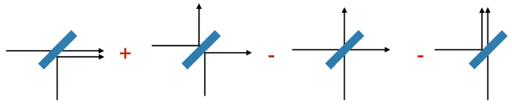
Figure 2: Diagram showing four different ways for two photons to interact on a beam splitter. The signs correspond to signs in front of terms in Eq. (7)

In HOM interference, we are often interested in the coincidence probability, that is, the probability of detecting one photon in each output port of the beam splitter. To compute this, we must take into account the distinguishability of the input photons. In the next section, we consider distinguishability in the polarization degree of freedom.

3 Polarization distinguishability

Just like classical light, an individual photon can be described as having horizontal ($H$) or vertical ($V$) polarization, or a superposition of the two ($\alpha H+\beta V$, where $\alpha$ and $\beta$ are complex numbers satisfying $|\alpha|^{2}+|\beta|^{2}=1$). In this section, we consider how the polarization of the input photons influences the HOM coincidence probability.

3.1 Distinguishable photons

First consider two photons with orthogonal polarizations, $H$ and $V$. Also assume that all other properties of the photons (spectrum, arrival time, transverse spatial mode, etc.) are identical. Two photons with orthogonal polarizations are said to be distinguishable. In this scenario, where $j=H$ and $k=V$, the output state is

$$|\psi^{\mathrm{out}}\rangle_{ab}={} \frac{1}{2}\left(\hat{a}^{\dagger}_{H}\hat{a}^{\dagger}_{V}+\hat{a}^{\dagger}_{V}\hat{b}^{\dagger}_{H}-\hat{a}^{\dagger}_{H}\hat{b}^{\dagger}_{V}-\hat{b}^{\dagger}_{H}\hat{b}^{\dagger}_{V}\right)|0\rangle_{ab}$$ (8)

$$={} \frac{1}{2}\left(|1;H\rangle_{a}|1;V\rangle_{a}+|1;V\rangle_{a}|1;H\rangle_{b}-|1;H\rangle_{a}|1;V\rangle_{b}-|1;H\rangle_{b}|1;V\rangle_{b}\right)\,.$$ (9)

The first term contains both photons in mode $a$, the second and third terms contain only one photon in each mode $a$ and $b$, and the fourth term contains both photons in mode $b$.

We can compute the coincidence probability from the probability amplitudes in front of terms with only one photon in each output port, i.e., the two middle terms in Eq. (9). The coincidence probability is therefore $p=|1/2|^{2}+|{-}1/2|^{2}=1/2$.

3.2 Indistinguishable photons

Now consider that the two photons have the same polarization, $j=k=H$. All other things being equal (spectrum, arrival time, transverse spatial mode, etc.), two photons with the same polarization are said to be indistinguishable. In this scenario, the output state is

$$|\psi^{\mathrm{out}}\rangle_{ab}={} \left(\hat{a}^{\dagger}_{H}\hat{a}^{\dagger}_{H}+\hat{a}^{\dagger}_{H}\hat{b}^{\dagger}_{H}-\hat{a}^{\dagger}_{H}\hat{b}^{\dagger}_{H}-\hat{b}^{\dagger}_{H}\hat{b}^{\dagger}_{H}\right)|0\rangle_{ab}$$ (10)

$$={} \left(\hat{a}^{\dagger}_{H}\hat{a}^{\dagger}_{H}-\hat{b}^{\dagger}_{H}\hat{b}^{\dagger}_{H}\right)|0\rangle_{ab}$$ (11)

$$={} \frac{1}{\sqrt{2}}\left(|2;H\rangle_{a}-|2;H\rangle_{b}\right)\,.$$ (12)

Notice that the two middle terms in Eq. (10) cancel, but the state still comes out normalized because $(\hat{a}^{\dagger})^{n}|0\rangle=\sqrt{n!}|n\rangle$. The first term in Eq. (12) has both photons in mode $a$ and the second term has both photons in mode $b$, but there are no terms corresponding to one photon in each mode $a$ and $b$. Compare this with the output state for distinguishable photons in Eq. (9). Incidentally, the state in Eq. (12) is sometimes called a two-photon N00N state, i.e., $|N\rangle|0\rangle+|0\rangle|N\rangle$ where $N=2$ [7].

Here, the coincidence probability of detecting one photon in each output mode is $p=0$. So we see that when two indistinguishable photons interfere on a beam splitter of reflectivity $\eta=1/2$, the amplitudes for “both transmitted” and “both reflected” perfectly cancel out.

4 Temporal distinguishability

Until now, we implicitly considered photons with the same spectral and temporal properties (their details were thus not relevant to our analysis). We now extend our analysis to include the spectral profile of the photons, characterized by the spectral amplitude function $\phi(\omega)$, and the relative arrival times of the photons, parametrized by the time delay $\tau$. By controlling the time delays between two such photons, it is possible to tune their level of distinguishability. This is shown schematically in Figure 3.

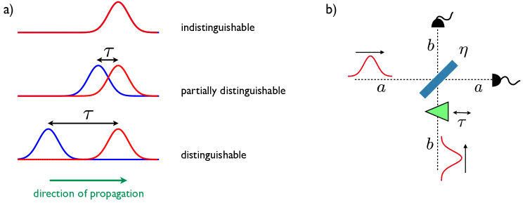
Figure 3: a) Changing the time delay $\tau$ between two photons with finite bandwidths changes how distinguishable they are. b) A time delay in mode $b$ might be introduced by sending the photon in that mode through a prism that introduces a phase shift.

4.1 Photons with arbitrary spectra

The quantum state for a photon with spectral amplitude function $\phi(\omega)$, in beam splitter mode $a$, is

$$|1;\phi\rangle_{a}=\int d\omega\phi(\omega)\hat{a}^{\dagger}(\omega)|0\rangle_{a}\,,$$ (13)

where $\hat{a}^{\dagger}(\omega)$ represents a creation operator acting on a single frequency mode $\omega$. The state is normalized such that $\int d\omega|\phi(\omega)|^{2}=1$.

Now consider two input photons with arbitrary spectral amplitude functions $\phi$ and $\varphi$. The two-photon input state is

$$|\psi^{\mathrm{in}}\rangle_{ab}={} |1;\phi\rangle_{a}|1;\varphi\rangle_{b}$$ (14)

$$={} \int d\omega_{1}\phi(\omega_{1})\hat{a}^{\dagger}(\omega_{1})\int d\omega_{2}\varphi(\omega_{2})\hat{b}^{\dagger}(\omega_{2})|0\rangle_{ab}\,.$$ (15)

We are interested in how the coincidence probability changes as a function of the overlap between the photons. We thus introduce a time delay in, say, mode $b$. In practice, this might be done by sending the photon in mode $b$ through a prism that introduces a phase shift (see Figure 3 b)), or perhaps by forcing it to take a longer path. The time delay has the following action on the creation operator:

$$\hat{b}^{\dagger}(\omega)\rightarrow\hat{b}^{\dagger}(\omega)\mathrm{e}^{-i\omega\tau}\,.$$ (16)

The time-delayed state is

$$|\psi^{\mathrm{td}}\rangle_{ab}={}\int d\omega_{1}\phi(\omega_{1})\hat{a}^{\dagger}(\omega_{1})\int d\omega_{2}\varphi(\omega_{2})\hat{b}^{\dagger}(\omega_{2})\mathrm{e}^{-i\omega_{2}\tau}|0\rangle_{ab}\,.$$ (17)

The beam splitter acts on each frequency mode independently, and we’ll assume that the reflectivity is not frequency-dependent. The beam splitter unitary thus acts on the creation operators as follows:

$$\hat{a}^{\dagger}(\omega)\xrightarrow{\hat{U}_{\textsc{bs}}}{} \sqrt{1-\eta}\hat{a}^{\dagger}(\omega)+\sqrt{\eta}\hat{b}^{\dagger}(\omega)$$ (18)

$$\hat{b}^{\dagger}(\omega)\xrightarrow{\hat{U}_{\textsc{bs}}}{} \sqrt{\eta}\hat{a}^{\dagger}(\omega)-\sqrt{1-\eta}\hat{b}^{\dagger}(\omega)\,.$$ (19)

After passing through a beam splitter with $\eta=1/2$, the output state of the two photons is

$$|\psi^{\mathrm{out}}\rangle_{ab}={} \hat{U}_{\textsc{bs}}|\psi^{\mathrm{td}}\rangle_{ab}$$ (20)

$$={} \frac{1}{2}\int d\omega_{1}\phi(\omega_{1})\left(\hat{a}^{\dagger}(\omega_{1})+\hat{b}^{\dagger}(\omega_{1})\right)\int d\omega_{2}\varphi(\omega_{2})\left(\hat{a}^{\dagger}(\omega_{2})-\hat{b}^{\dagger}(\omega_{2})\right)\mathrm{e}^{-i\omega_{2}\tau}|0\rangle_{ab}$$ (21)

$$\begin{split}={}&\frac{1}{2}\int d\omega_{1}\phi(\omega_{1})\int d\omega_{2}\varphi(\omega_{2})\mathrm{e}^{-i\omega_{2}\tau}\\ &\times\left(\hat{a}^{\dagger}(\omega_{1})\hat{a}^{\dagger}(\omega_{2})+\hat{a}^{\dagger}(\omega_{2})\hat{b}^{\dagger}(\omega_{1})-\hat{a}^{\dagger}(\omega_{1})\hat{b}^{\dagger}(\omega_{2})-\hat{b}^{\dagger}(\omega_{1})\hat{b}^{\dagger}(\omega_{2})\right)|0\rangle_{ab}\,.\end{split}$$ (22)

Earlier, when we considered photons of a single frequency, it was simple to read off the coincidence probability from the state. Here, it is a bit more tricky so we should calculate it explicitly. We’ll model each detector as having a flat frequency response. The projector describing detection in mode $a$ is given by

$$\hat{P}_{a}=\int d\omega\hat{a}^{\dagger}(\omega)|0\rangle_{a}\langle 0|_{a}\hat{a}(\omega)\,,$$ (23)

and the projector describing detection in mode $b$ is given by

$$\hat{P}_{b}=\int d\omega\hat{b}^{\dagger}(\omega)|0\rangle_{b}\langle 0|_{b}\hat{b}(\omega)\,.$$ (24)

The coincidence probability of detecting one photon in each mode is

$$p={} \mathrm{Tr}[|\psi^{\mathrm{out}}\rangle_{ab}\langle\psi^{\mathrm{out}}|_{ab}\hat{P}_{a}\otimes\hat{P}_{b}]=\langle\psi^{\mathrm{out}}|_{ab}\hat{P}_{a}\otimes\hat{P}_{b}|\psi^{\mathrm{out}}\rangle_{ab}\,.$$ (25)

For two photons with arbitrary spectral amplitude functions $\phi$ and $\varphi$, the coincidence probability is

$$\begin{split}p_{\mathrm{arb}}={}&\Bigg{[}\frac{1}{2}\int d\omega_{1}\int d\omega_{2}\phi^{*}(\omega_{1})\varphi^{*}(\omega_{2})\mathrm{e}^{i\omega_{2}\tau}\\ &\times\langle 0|\left(\hat{a}(\omega_{1})\hat{a}(\omega_{2})+\hat{a}(\omega_{2})\hat{b}(\omega_{1})-\hat{a}(\omega_{1})\hat{b}(\omega_{2})-\hat{b}(\omega_{1})\hat{b}(\omega_{2})\right)\Bigg{]}\\ &\times\Bigg{[}\int d\omega_{a}\hat{a}^{\dagger}(\omega_{a})|0\rangle_{a}\langle 0|_{a}\hat{a}(\omega_{a})\int d\omega_{b}\hat{b}^{\dagger}(\omega_{b})|0\rangle_{b}\langle 0|_{b}\hat{b}(\omega_{b})\Bigg{]}\\ &\times\Bigg{[}\frac{1}{2}\int d\omega^{\prime}_{1}\int d\omega^{\prime}_{2}\phi(\omega^{\prime}_{1})\varphi(\omega^{\prime}_{2})\mathrm{e}^{-i\omega^{\prime}_{2}\tau}\\ &\times\left(\hat{a}^{\dagger}(\omega^{\prime}_{1})\hat{a}^{\dagger}(\omega^{\prime}_{2})+\hat{a}^{\dagger}(\omega^{\prime}_{2})\hat{b}^{\dagger}(\omega^{\prime}_{1})-\hat{a}^{\dagger}(\omega^{\prime}_{1})\hat{b}^{\dagger}(\omega^{\prime}_{2})-\hat{b}^{\dagger}(\omega^{\prime}_{1})\hat{b}^{\dagger}(\omega^{\prime}_{2})\right)|0\rangle_{ab}\Bigg{]}\,,\end{split}$$ (26)

where all we did so far was insert Eqs. (22), (23), and (24) into Eq. (25). Reshuffling some parts, we can write

$$\begin{split}p_{\mathrm{arb}}={}&\frac{1}{4}\int d\omega_{a}\int d\omega_{b}\int d\omega_{1}\int d\omega_{2}\int d\omega^{\prime}_{1}\int d\omega^{\prime}_{2}\phi^{*}(\omega_{1})\varphi^{*}(\omega_{2})\phi(\omega^{\prime}_{1})\varphi(\omega^{\prime}_{2})\mathrm{e}^{i(\omega_{2}-\omega^{\prime}_{2})\tau}\\ &\times\langle 0|_{ab}\left(\hat{a}(\omega_{1})\hat{a}(\omega_{2})+\hat{a}(\omega_{2})\hat{b}(\omega_{1})-\hat{a}(\omega_{1})\hat{b}(\omega_{2})-\hat{b}(\omega_{1})\hat{b}(\omega_{2})\right)\hat{a}^{\dagger}(\omega_{a})\hat{b}^{\dagger}(\omega_{b})|0\rangle_{ab}\\ &\times\langle 0|_{ab}\hat{a}(\omega_{a})\hat{b}(\omega_{b})\left(\hat{a}^{\dagger}(\omega^{\prime}_{1})\hat{a}^{\dagger}(\omega^{\prime}_{2})+\hat{a}^{\dagger}(\omega^{\prime}_{2})\hat{b}^{\dagger}(\omega^{\prime}_{1})-\hat{a}^{\dagger}(\omega^{\prime}_{1})\hat{b}^{\dagger}(\omega^{\prime}_{2})-\hat{b}^{\dagger}(\omega^{\prime}_{1})\hat{b}^{\dagger}(\omega^{\prime}_{2})\right)|0\rangle_{ab}\,.\end{split}$$ (27)

Terms with an odd number of operators in one mode, e.g. $\langle 0|_{ab}\hat{a}\hat{a}\hat{a}^{\dagger}\hat{b}^{\dagger}|0\rangle_{ab}$ and $\langle 0|_{ab}\hat{b}\hat{b}\hat{a}^{\dagger}\hat{b}^{\dagger}|0\rangle_{ab}$, go to zero, while terms such as $\langle 0|_{ab}\hat{a}\hat{b}\hat{a}^{\dagger}\hat{b}^{\dagger}|0\rangle_{ab}$ give delta functions:

$$\begin{split}p_{\mathrm{arb}}={}&\frac{1}{4}\int d\omega_{a}\int d\omega_{b}\int d\omega_{1}\int d\omega_{2}\int d\omega^{\prime}_{1}\int d\omega^{\prime}_{2}\phi^{*}(\omega_{1})\varphi^{*}(\omega_{2})\phi(\omega^{\prime}_{1})\varphi(\omega^{\prime}_{2})\mathrm{e}^{i(\omega_{2}-\omega^{\prime}_{2})\tau}\\ &\times\left(\delta(\omega_{2}-\omega_{a})\delta(\omega_{1}-\omega_{b})-\delta(\omega_{1}-\omega_{a})\delta(\omega_{2}-\omega_{b})\right)\\ &\times\left(\delta(\omega^{\prime}_{2}-\omega_{a})\delta(\omega^{\prime}_{1}-\omega_{b})-\delta(\omega^{\prime}_{1}-\omega_{a})\delta(\omega^{\prime}_{2}-\omega_{b})\right)\,.\end{split}$$ (28)

Using the delta functions to evaluate the integrals over $\omega_{a}$ and $\omega_{b}$ gives an expression with two terms:

$$\begin{split}p_{\mathrm{arb}}={}&\frac{1}{2}\int d\omega_{1}\int d\omega_{2}\int d\omega^{\prime}_{1}\int d\omega^{\prime}_{2}\phi^{*}(\omega_{1})\varphi^{*}(\omega_{2})\phi(\omega^{\prime}_{1})\varphi(\omega^{\prime}_{2})\mathrm{e}^{i(\omega_{2}-\omega^{\prime}_{2})\tau}\\ &\times\left(\delta(\omega_{2}-\omega^{\prime}_{2})\delta(\omega_{1}-\omega^{\prime}_{1})-\delta(\omega_{1}-\omega^{\prime}_{2})\delta(\omega_{2}-\omega^{\prime}_{1})\right)\,.\end{split}$$ (29)

Using the remaining delta functions to evaluate the integrals over $\omega^{\prime}_{1}$ and $\omega^{\prime}_{2}$, and taking advantage of the normalization condition $\int d\omega|\phi(\omega)|^{2}=1$, gives

$$\begin{split}p_{\mathrm{arb}}={}&\frac{1}{2}-\frac{1}{2}\int d\omega_{1}\phi^{*}(\omega_{1})\varphi(\omega_{1})\mathrm{e}^{-i\omega_{1}\tau}\int d\omega_{2}\varphi^{*}(\omega_{2})\phi(\omega_{2})\mathrm{e}^{i\omega_{2}\tau}\,.\end{split}$$ (30)

If $\phi(\omega)=\varphi(\omega)$, this expression simplifies to

$$\begin{split}p_{\mathrm{arb}}={}&\frac{1}{2}-\frac{1}{2}\int d\omega_{1}|\phi(\omega_{1})|^{2}\mathrm{e}^{-i\omega_{1}\tau}\int d\omega_{2}|\phi(\omega_{2})|^{2}\mathrm{e}^{i\omega_{2}\tau}\,.\end{split}$$ (31)

4.1.1 Example: Gaussian photons

Consider two photons with Gaussian spectral amplitude functions,

$$\phi_{i}(\omega)=\frac{1}{(\pi)^{1/4}\sqrt{\sigma_{i}}}e^{-\frac{\left(\omega-\bar{\omega}_{i}\right){}^{2}}{2\sigma_{i}^{2}}}\,;~{}~{}~{}~{}~{}(i=a,b)\,,$$ (32)

where $\bar{\omega}_{i}$ is the central frequency of photon $i$, $\sigma_{i}$ defines its spectral width, and the normalization was chosen such that $\int d\omega|\phi_{i}(\omega)|^{2}=1$. From Eq. (30), the coincidence probability is

$$\begin{split}p_{\mathrm{arb,gauss}}={}&\frac{1}{2}-\frac{1}{2\pi\sigma_{a}\sigma_{b}}\left(\int d\omega_{1}e^{-\frac{\left(\omega_{1}-\bar{\omega}_{a}\right){}^{2}}{2\sigma_{a}^{2}}}e^{-\frac{\left(\omega_{1}-\bar{\omega}_{b}\right){}^{2}}{2\sigma_{b}^{2}}}\mathrm{e}^{-i\omega_{1}\tau}\right)\left(\int d\omega_{2}e^{-\frac{\left(\omega_{2}-\bar{\omega}_{a}\right){}^{2}}{2\sigma_{a}^{2}}}e^{-\frac{\left(\omega_{2}-\bar{\omega}_{b}\right){}^{2}}{2\sigma_{b}^{2}}}\mathrm{e}^{i\omega_{2}\tau}\right)\,.\end{split}$$ (33)

The Fourier Transforms can be evaluated using your favourite method (mine is Mathematica). The coincidence probability simplifies to

$$\begin{split}p_{\mathrm{arb,gauss}}={}&\frac{1}{2}-\frac{\sigma_{a}\sigma_{b}}{(\sigma_{a}^{2}+\sigma_{b}^{2})}e^{-\frac{\sigma_{a}^{2}\sigma_{b}^{2}\tau^{2}+(\bar{\omega}_{a}-\bar{\omega}_{b})^{2}}{\sigma_{a}^{2}+\sigma_{b}^{2}}}\,.\end{split}$$ (34)

If the Gaussians are equal, that is $\phi_{a}=\phi_{b}$, we have

$$\begin{split}p_{\mathrm{arb,gauss}}={}&\frac{1}{2}-\frac{1}{2}\mathrm{e}^{-\frac{\sigma_{a}^{2}\tau^{2}}{2}}\,.\end{split}$$ (35)

4.1.2 Example: Sinc-shaped photons

Consider two photons with a sinc spectral amplitude function,

$$\varphi_{i}(\omega)=\sqrt{\frac{A_{i}}{\pi}}\mathrm{sinc}\left(A_{i}(\omega-\bar{\omega}_{i})\right)\,;~{}~{}~{}~{}~{}(i=a,b)\,,$$ (36)

where $\bar{\omega}_{i}$ is the central frequency of photon $i$, $A_{i}^{-1}$ defines its spectral width, and the normalization was chosen such that $\int d\omega|\varphi_{i}(\omega)|^{2}=1$. From Eq. (30), the coincidence probability is

$$\begin{split}p_{\mathrm{arb,sinc}}={}&\frac{1}{2}-\frac{A_{a}A_{b}}{2\pi^{2}}\left(\int d\omega_{1}\mathrm{sinc}\left(A_{a}(\omega_{1}-\bar{\omega}_{1})\right)\mathrm{sinc}\left(A_{b}(\omega_{1}-\bar{\omega}_{1})\right)\mathrm{e}^{-i\omega_{1}\tau}\right)\\ &\times\left(\int d\omega_{2}\mathrm{sinc}\left(A_{a}(\omega_{2}-\bar{\omega}_{2})\right)\mathrm{sinc}\left(A_{b}(\omega_{2}-\bar{\omega}_{2})\right)\mathrm{e}^{i\omega_{2}\tau}\right)\,.\end{split}$$ (37)

Computing the Fourier Transforms, in the case where $\varphi_{a}=\varphi_{b}$, the coincidence probability simplifies to

$$\begin{split}p_{\mathrm{arb,sinc}}={}&\frac{1}{2}-\frac{1}{8A_{a}^{2}}\left(|\tau|-\left|\frac{\tau}{2}-A_{a}\right|-\left|\frac{\tau}{2}+A_{a}\right|\right)^{2}\,.\end{split}$$ (38)

Figure 4 compares the coincidence probabilities, Eqs. (35) and (38), for photons with Gaussian and sinc spectral amplitude functions respectively.

SEPARABLE PHOTONS

Figure 4: The coincidence probability for separable photons, as a function of time delay $\tau$. The solid line is $p_{\mathrm{arb,gauss}}$ defined in Eq. (35) for $\sigma_{a}=10^{-12}$ rad/s, and the dashed line is $p_{\mathrm{arb,sinc}}$ defined in Eq. (38) for $A_{a}=1/\sigma_{a}\sqrt{2\gamma}$ where $\sigma_{a}=10^{-12}$ rad/s and $\gamma=0.193$. This value of $\gamma$ ensures that the Gaussian and sinc spectral amplitude functions have the same widths, for comparison.

4.2 Spectrally entangled photons

In the previous section, we considered two photons with arbitrary, but separable, spectral amplitude profiles. More generally, however, the spectral amplitudes of two photons can be correlated— that is, the photons can be entangled in the spectral degree of freedom. The nature of this spectral entanglement is captured by the joint spectral amplitude (JSA) function $f(\omega_{1},\omega_{2})$. The quantum state of two spectrally entangled photons is

$$|\psi^{\mathrm{in}}\rangle_{ab}={} \int d\omega_{1}\int d\omega_{2}f(\omega_{1},\omega_{2})\hat{a}^{\dagger}(\omega_{1})\hat{b}^{\dagger}(\omega_{2})|0\rangle_{ab}\,.$$ (39)

Notice that for $f(\omega_{1},\omega_{2})=\phi(\omega_{1})\varphi(\omega_{2})$, this state reduces to the separable state in Eq. (15). Entangled photons can be sent onto a beam splitter in exactly the same way as separable photons, but the way they interfere will also depend on the nature of their entanglement.

As before, to calculate the HOM dip, we begin by introducing a time delay $\tau$ in mode $b$, by applying the transformation in Eq. (16). We then model how the photons interact via the beam splitter by applying the beam splitter unitary in Eq. (18) to the time-delayed state. We finally calculate the coincidence probability, as defined in Eq. (25), using projectors, defined in Eqs. (23) and (24), that describe detection in modes $a$ and $b$. The steps are identical to those in Section 4.1, and yield the coincidence probability:

$$\begin{split}p_{\mathrm{ent}}={}&\frac{1}{2}-\frac{1}{2}\int d\omega_{1}\int d\omega_{2}f^{*}(\omega_{1},\omega_{2})f(\omega_{2},\omega_{1})\mathrm{e}^{i(\omega_{2}-\omega_{1})\tau}\,.\end{split}$$ (40)

In fact, this is equivalent to the coincidence probability in Eq. (30) when $f(\omega_{1},\omega_{2})=\phi(\omega_{1})\varphi(\omega_{2})$. In general, however, $f(\omega_{1},\omega_{2})$ will not take such a nice form, and the integrals in Eq. (40) will need to be evaluated numerically.

It can sometimes be useful to express the JSA in terms of its’ Schmidt decomposition,

$$f(\omega_{1},\omega_{2})={} \sum_{k}u_{k}\phi_{k}(\omega_{1})\varphi_{k}(\omega_{2})\,,$$ (41)

where the Schmidt modes $\phi_{k}(\omega)$ and $\varphi_{k}(\omega)$ each form a discrete basis of complex orthonormal functions ($\int d\omega\phi^{*}_{k}(\omega)\phi_{k^{\prime}}(\omega)=\int d\omega\varphi^{*}_{k}(\omega)\varphi_{k^{\prime}}(\omega)=\delta_{kk^{\prime}}$), and the Schmidt coefficients ${u}_{k}$ are real and satisfy $\sum_{k}{u}_{k}^{2}=1$ if $f(\omega_{1},\omega_{2})$ is normalized. The coincidence probability can then be expressed in terms of the Schmidt coefficients and Schmidt modes as

$$p_{\mathrm{ent}}={} \frac{1}{2}-\frac{1}{2}\sum_{k,k^{\prime}}u_{k}u_{k^{\prime}}\int d\omega_{1}\phi^{*}_{k}(\omega_{1})\varphi_{k^{\prime}}(\omega_{1})\mathrm{e}^{-i\omega_{1}\tau}\int d\omega_{2}\varphi^{*}_{k}(\omega_{2})\phi_{k^{\prime}}(\omega_{2})\mathrm{e}^{i\omega_{2}\tau}\,.$$ (42)

4.2.1 Example: SPDC pumped by a pulsed pump laser

The joint spectral amplitude for photons generated via spontaneous parametric downconversion is

$$f(\omega_{1},\omega_{2})\propto\Phi(\omega_{1},\omega_{2})\alpha(\omega_{1}+\omega_{2})\,,$$ (43)

such that $\int d\omega_{1}d\omega_{2}|f(\omega_{1},\omega_{2})|^{2}=1$, where $\Phi(\omega_{1},\omega_{2})$ is known as the phase-matching function and $\alpha(\omega_{1}+\omega_{2})$ is the pump amplitude function [8].

A typical SPDC crystal of length $L$ generates a phase-matching function with a sinc profile:

$$\Phi_{\mathrm{sinc}}(\omega_{1},\omega_{2})=\mathrm{sinc}\left(\frac{\Delta k(\omega_{1},\omega_{2})L}{2}\right)\,,$$ (44)

where $\Delta k(\omega_{1},\omega_{2})=k_{p}(\omega_{1}+\omega_{2})-k_{1}(\omega_{1})+k_{2}(\omega_{2})$, and $k_{i}(\omega)$ are the wave numbers associated with the respective fields.

To simplify calculations, we can Taylor expand $\Delta k(\omega_{1},\omega_{2})$ to first order:

$$\Delta k(\omega_{1},\omega_{2})=k_{1,0}+k_{2,0}-k_{p,0}+k^{\prime}_{1}(\omega_{1}-\bar{\omega})+k^{\prime}_{2}(\omega_{2}-\bar{\omega})-k^{\prime}_{p}(\omega_{1}+\omega_{2}-2\bar{\omega})\,,$$ (45)

where $k_{p,0}=k_{p}(2\bar{\omega})$, $k_{1/2,0}=k_{1/2}(\bar{\omega})$, $k_{p}^{\prime}=\partial_{p}(\omega)/\partial\omega|_{\omega=2\bar{\omega}}$, and $k_{1/2}^{\prime}=\partial_{1/2}(\omega)/\partial\omega|_{\omega=\bar{\omega}}$. This approximation is valid in many regimes. We can then write

$$\Phi_{\mathrm{sinc}}(\omega_{1},\omega_{2})=\mathrm{sinc}\left(A\omega_{1}+B\omega_{2}-C\right)\,,$$ (46)

where

$$A={} \frac{L}{2}(k^{\prime}_{1}-k^{\prime}_{p})$$ (47)

$$B={} \frac{L}{2}(k^{\prime}_{2}-k^{\prime}_{p})$$ (48)

$$C={} \frac{L}{2}(k_{1,0}+k_{2,0}-k_{p,0}+(k^{\prime}_{1}+k^{\prime}_{2}-2k^{\prime}_{p})\bar{\omega})\,.$$ (49)

For comparison, it is useful to define a Gaussian phase-matching function of the same width:

$$\Phi_{\mathrm{gauss}}(\omega_{1},\omega_{2})=e^{-\gamma\left(A\omega_{1}+B\omega_{2}-C\right)^{2}}\,,$$ (50)

where the parameter $\gamma=0.193$ ensures that the Gaussian and sinc functions have the same widths. Gaussian phase-matching functions were originally used in the literature to simplify calculations. But, more recently, methods have been developed to generate them in practice [9, 10, 11, 12, 13]. In combination with the right set of parameters (A, B, C, and $\sigma$), Gaussian phase-matching functions make it possible to generate separable joint spectral amplitudes via SPDC (see Fig. 5 a))

For a pulsed pump laser, it is common to assume a Gaussian pump amplitude function:

$$\alpha(\omega)=e^{-\frac{(\omega-\bar{\omega})^{2}}{2\sigma^{2}}}\,,$$ (51)

where $\bar{\omega}$ is the central frequency of the pump, and $\sigma$ defines the spectral width.

We define the corresponding joint spectral amplitudes:

$$f_{\mathrm{gauss}}(\omega_{1},\omega_{2})\propto{} \Phi_{\mathrm{gauss}}(\omega_{1},\omega_{2})\alpha(\omega_{1}+\omega_{2})$$ (52)

$$f_{\mathrm{sinc}}(\omega_{1},\omega_{2})\propto{} \Phi_{\mathrm{sinc}}(\omega_{1},\omega_{2})\alpha(\omega_{1}+\omega_{2})\,,$$ (53)

which are plotted in Figure 5.

Figure 6 compares the coincidence probabilities for photons from an SPDC source pumped by a pulsed laser, with Gaussian and sinc phase matching functions functions respectively.

a)                                                                        b)

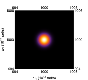
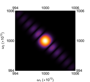
Figure 5: Joint spectral amplitudes: a) $|f_{\mathrm{gauss}}(\omega_{1},\omega_{2})|$, and b) $|f_{\mathrm{sinc}}(\omega_{1},\omega_{2})|$, with $A=1/\sigma\sqrt{2\gamma}$, $B=-A$, $C=0$, $\gamma=0.193$, $\sigma=10^{12}$ rad/s, and $\bar{\omega}=10^{15}$ rad/s.

SPDC PAIR (PULSED)

Figure 6: The coincidence probability for photons from an SPDC source pumped by a pulsed laser, Eq. (40), as a function of time delay $\tau$. The solid line is for $f_{\mathrm{gauss}}(\omega_{1},\omega_{2})$ defined in Eq. (52), and the dashed line is for $f_{\mathrm{sinc}}(\omega_{1},\omega_{2})$ defined in Eq. (53). All parameters are the same as for Figure 5.

4.2.2 Example: SPDC pumped by a CW pump laser

For a nonlinear source pumped by a continuous wave (CW) laser at frequency $2\bar{\omega}$, the joint spectral amplitude takes the form

$$f(\omega_{1},\omega_{2})\propto\Phi(\omega_{1},\omega_{2})\delta(\omega_{1}+\omega_{2}-2\bar{\omega})\,,$$ (54)

such that $\int d\omega_{1}d\omega_{2}|f(\omega_{1},\omega_{2})|^{2}=1$. The coincidence probability in Eq. (40) then simplifies to

$$p_{\mathrm{cw}}={} \frac{1}{2}-\frac{1}{2}\int d\omega g^{*}(-\omega)g(\omega)\mathrm{e}^{i2\omega\tau}\,,$$ (55)

where $g(\omega)\propto\Phi(\bar{\omega}-\omega,\bar{\omega}+\omega)$, such that $\int d\omega|g(\omega)|^{2}=1$.

Figure 7 compares the coincidence probabilities for photons from an SPDC source pumped by a CW laser, with Gaussian and sinc phase matching functions functions respectively.

SPDC PAIR (CW)

Figure 7: The coincidence probability for entangled photons from an SPDC source pumped by a CW laser, Eq. (55), as a function of time delay $\tau$. The solid line is for $\Phi_{\mathrm{gauss}}(\omega_{1},\omega_{2})$ defined in Eq. (50), and the dashed line is for $\Phi_{\mathrm{sinc}}(\omega_{1},\omega_{2})$ defined in Eq. (46). All parameters are the same as for Figure 5.

4.3 Spectrally mixed states

In the previous sections, we considered single photons and photon pairs in spectrally pure states. It is possible, however, for a photon to be in a mixture of different spectral amplitude functions $\phi_{k}(\omega)$. This can be represented by the density matrix

$$\rho_{\phi}={} \sum_{k}q_{k}|1;\phi_{k}\rangle_{a}\langle 1;\phi_{k}|_{a}\,,$$ (56)

where

$$|1;\phi\rangle_{a}={} \int d\omega\phi(\omega)\hat{a}^{\dagger}(\omega)|0\rangle_{a}\,,$$ (57)

is the quantum state for a single photon in a spectral mode defined by the spectral amplitude function $\phi(\omega)$. The density matrix $\rho_{\phi}$ can be realized in one of two ways: 1) as a probabilistic preparation on the pure state $|1;\phi_{k}\rangle$ with probability $q_{k}$, or 2) as the reduced density matrix of a spectrally entangled two-photon state, such as Eq. (39) (see Appendix A for details).

Spectrally mixed photons can be sent onto a beam splitter in exactly the same way as separable or entangled photons. The density operator for a two-photon input state can be written as

$$\rho^{\mathrm{in}}={} \rho_{\phi}\otimes\rho_{\varphi}$$ (58)

$$={} \sum_{k}q_{k}|1;\phi_{k}\rangle_{a}\langle 1;\phi_{k}|_{a}\otimes\sum_{k}q^{\prime}_{k^{\prime}}|1;\varphi_{k^{\prime}}\rangle_{b}\langle 1;\varphi_{k^{\prime}}|_{b}$$ (59)

$$={} \sum_{kk^{\prime}}q_{k}q^{\prime}_{k^{\prime}}\left(|1;\phi_{k}\rangle_{a}|1;\varphi_{k^{\prime}}\rangle_{b}\right)\left(\langle 1;\phi_{k}|_{a}\langle 1;\varphi_{k^{\prime}}|_{b}\right)\,.$$ (60)

As before, the next step is to introduce a time delay $\tau$ in mode $b$, by applying the transformation in Eq. (16), and then model how the photons interact via the beam splitter by applying the beam splitter unitary in Eq. (18) to the time-delayed state. But notice that the state $|1;\phi_{k}\rangle_{a}|1;\varphi_{k^{\prime}}\rangle_{b}$ is just the state of two photons with arbitrary spectral amplitude functions $\phi_{k}$ and $\varphi_{k^{\prime}}$ that we saw in Eq. (14) in Section 4.1. Due to the linearity of quantum mechanics, we can simply use the result from Section 4.1 to write the output density operator

$$\rho^{\mathrm{out}}={} \sum_{kk^{\prime}}q_{k}q^{\prime}_{k^{\prime}}|\psi_{kk^{\prime}}^{\mathrm{out}}\rangle_{ab}\langle\psi_{kk^{\prime}}^{\mathrm{out}}|_{ab}\,,$$ (61)

where

$$\begin{split}|\psi_{kk^{\prime}}^{\mathrm{out}}\rangle_{ab}={}&\frac{1}{2}\int d\omega_{1}\phi_{k}(\omega_{1})\int d\omega_{2}\varphi_{k^{\prime}}(\omega_{2})\mathrm{e}^{-i\omega_{2}\tau}\\ &\times\left(\hat{a}^{\dagger}(\omega_{1})\hat{a}^{\dagger}(\omega_{2})+\hat{a}^{\dagger}(\omega_{2})\hat{b}^{\dagger}(\omega_{1})-\hat{a}^{\dagger}(\omega_{1})\hat{b}^{\dagger}(\omega_{2})-\hat{b}^{\dagger}(\omega_{1})\hat{b}^{\dagger}(\omega_{2})\right)|0\rangle_{ab}\,.\end{split}$$ (62)

This is equivalent to Eq. (22) for $\phi(\omega)=\phi_{k}(\omega)$ and $\varphi(\omega)=\varphi_{k^{\prime}}(\omega)$. The coincidence probability of getting one photon in each mode is

$$p_{\mathrm{mix}}={} \mathrm{Tr}[\rho^{\mathrm{out}}\hat{P}_{a}\otimes\hat{P}_{b}]$$ (63)

$$={} \sum_{kk^{\prime}}q_{k}q^{\prime}_{k^{\prime}}\langle\psi_{kk^{\prime}}^{\mathrm{out}}|_{ab}\hat{P}_{a}\otimes\hat{P}_{b}|\psi_{kk^{\prime}}^{\mathrm{out}}\rangle_{ab}\,,$$ (64)

where $\langle\psi_{kk^{\prime}}^{\mathrm{out}}|_{ab}\hat{P}_{a}\otimes\hat{P}_{b}|\psi_{kk^{\prime}}^{\mathrm{out}}\rangle_{ab}$ is the coincidence probability, defined in Eq. (25), for two photons with arbitrary spectral amplitude functions $\phi_{k}(\omega)$ and $\varphi_{k^{\prime}}(\omega)$. We can therefore replace $\langle\psi_{kk^{\prime}}^{\mathrm{out}}|_{ab}\hat{P}_{a}\otimes\hat{P}_{b}|\psi_{kk^{\prime}}^{\mathrm{out}}\rangle_{ab}$ with Eq. (30), for $\phi(\omega)=\phi_{k}(\omega)$ and $\varphi(\omega)=\varphi_{k^{\prime}}(\omega)$, to get

$$\begin{split}p_{\mathrm{mix}}={}&\frac{1}{2}-\frac{1}{2}\sum_{kk^{\prime}}q_{k}q^{\prime}_{k^{\prime}}\int d\omega_{1}\phi_{k}^{*}(\omega_{1})\varphi_{k^{\prime}}(\omega_{1})\mathrm{e}^{-i\omega_{1}\tau}\int d\omega_{2}\varphi_{k^{\prime}}^{*}(\omega_{2})\phi_{k}(\omega_{2})\mathrm{e}^{i\omega_{2}\tau}\,.\end{split}$$ (65)

4.3.1 Example: Independent SPDC sources

Consider two independent SPDC sources that generate the entangled states:

$$|\psi_{1}\rangle_{ab}={} \int d\omega_{1}\int d\omega_{2}f(\omega_{1},\omega_{2})\hat{a}^{\dagger}(\omega_{1})\hat{b}^{\dagger}(\omega_{2})|0\rangle_{ab}$$ (66)

$$|\psi_{2}\rangle_{cd}={} \int d\omega_{1}\int d\omega_{2}h(\omega_{1},\omega_{2})\hat{c}^{\dagger}(\omega_{1})\hat{d}^{\dagger}(\omega_{2})|0\rangle_{cd}\,.$$ (67)

To model a HOM experiment between photons in modes $a$ and $c$, we first compute the reduced density operators for those modes (see Appendix A):

$$\rho_{\phi}={} \mathrm{tr}_{b}\left[|\psi_{1}\rangle_{ab}\langle\psi_{1}|_{ab}\right]=\sum_{k}u_{1}^{2}|1;\phi_{k}\rangle_{a}\langle 1;\phi_{k}|_{a}$$ (68)

$$\rho_{\varphi}={} \mathrm{tr}_{d}\left[|\psi_{2}\rangle_{cd}\langle\psi_{2}|_{cd}\right]=\sum_{k}v_{1}^{2}|1;\varphi_{k}\rangle_{c}\langle 1;\varphi_{k}|_{c}\,,$$ (69)

where $\phi_{k}$ and $\varphi_{k}$ are defined in terms of the Schmidt decompositions of the joint spectral amplitudes:

$$f(\omega_{1},\omega_{2})={} \sum_{k}u_{k}\phi_{k}(\omega_{1})\phi^{\prime}_{k}(\omega_{2})$$ (70)

$$h(\omega_{1},\omega_{2})={} \sum_{k}v_{k}\varphi_{k}(\omega_{1})\varphi^{\prime}_{k}(\omega_{2})\,.$$ (71)

The coincidence probability, Eq. (65), becomes

$$\begin{split}p_{\mathrm{mix}}={}&\frac{1}{2}-\frac{1}{2}\sum_{kk^{\prime}}u^{2}_{k}v^{2}_{k^{\prime}}\int d\omega_{1}\phi_{k}^{*}(\omega_{1})\varphi_{k^{\prime}}(\omega_{1})\mathrm{e}^{-i\omega_{1}\tau}\int d\omega_{2}\varphi_{k^{\prime}}^{*}(\omega_{2})\phi_{k}(\omega_{2})\mathrm{e}^{i\omega_{2}\tau}\,.\end{split}$$ (72)

Figure 8 compares the coincidence probabilities for photons from two independent SPDC sources pumped by pulsed lasers, with Gaussian and sinc phase matching functions functions respectively.

MIXED STATES FROM INDEPENDENT SPDC SOURCES

Figure 8: The coincidence probability for photons from two independent SPDC sources pumped by pulsed lasers, Eq. (72), as a function of time delay $\tau$. The solid line is for $f(\omega_{1},\omega_{2})=h(\omega_{1},\omega_{2})=f_{\mathrm{gauss}}(\omega_{1},\omega_{2})$, where $f_{\mathrm{gauss}}(\omega_{1},\omega_{2})$ is defined in Eq. (52), and the dashed line is for $f(\omega_{1},\omega_{2})=h(\omega_{1},\omega_{2})=f_{\mathrm{sinc}}(\omega_{1},\omega_{2})$, where $f_{\mathrm{sinc}}(\omega_{1},\omega_{2})$ is defined in Eq. (53). All parameters are the same as for Figure 5.

4.3.2 Purity and Visibility

In the special case of mixed, identical, and separable photons, there is a nice relationship between the visibility of the HOM dip and the purity of the input photons.

The visibility of the HOM dip is given by

$$V=\frac{p_{\mathrm{max}}-p_{\mathrm{min}}}{p_{\mathrm{max}}}\,,$$ (73)

where

$$p_{\mathrm{max}}={} \lim_{\tau\rightarrow\infty}p_{\mathrm{mix}}=\frac{1}{2}$$ (74)

$$p_{\mathrm{min}}={} \lim_{\tau\rightarrow 0}p_{\mathrm{mix}}=\frac{1}{2}-\frac{1}{2}\sum_{kk^{\prime}}q_{k}q^{\prime}_{k^{\prime}}\int d\omega_{1}\phi_{k}^{*}(\omega_{1})\varphi_{k^{\prime}}(\omega_{1})\int d\omega_{2}\varphi_{k^{\prime}}^{*}(\omega_{2})\phi_{k}(\omega_{2})\,.$$ (75)

Given two photons with the same mixed density matrix ($\varphi_{k}=\phi_{k}$),

$$p_{\mathrm{min}}={} \frac{1}{2}-\frac{1}{2}\sum_{kk^{\prime}}q_{k}q_{k^{\prime}}\int d\omega_{1}\phi_{k}^{*}(\omega_{1})\phi_{k^{\prime}}(\omega_{1})\int d\omega_{2}\phi_{k^{\prime}}^{*}(\omega_{2})\phi_{k}(\omega_{2})$$ (76)

$$={} \frac{1}{2}-\frac{1}{2}\sum_{kk^{\prime}}q_{k}q_{k^{\prime}}\int d\omega_{1}\phi_{k}^{*}(\omega_{1})\phi_{k^{\prime}}(\omega_{1})\delta_{kk^{\prime}}$$ (77)

$$={} \frac{1}{2}-\frac{1}{2}\sum_{k}q^{2}_{k}\,.$$ (78)

In this case, the visibility is

$$V={} \frac{\frac{1}{2}-(\frac{1}{2}-\frac{1}{2}\sum_{k}q^{2}_{k})}{\frac{1}{2}}$$ (79)

$$={} \sum_{k}q^{2}_{k}\,.$$ (80)

The visibility is then equal to the purity of each photon

$$\mathrm{purity}={} \mathrm{tr}\left[\rho_{\phi}^{2}\right]$$ (81)

$$={} \mathrm{tr}\left[\sum_{k}q_{k}|1;\phi_{k}\rangle_{a}\langle 1;\phi_{k}|_{a}\sum_{k^{\prime}}q_{k^{\prime}}|1;\phi_{k^{\prime}}\rangle_{a}\langle 1;\phi_{k^{\prime}}|_{a}\right]$$ (82)

$$={} \sum_{kk^{\prime}}q_{k}q_{k^{\prime}}\delta_{kk^{\prime}}$$ (83)

$$={} \sum_{k}q^{2}_{k}\,.$$ (84)

5 (Not so) Final words

In this document, we introduced Hong-Ou-Mandel interference in terms of the photons’ distinguishability in the polarization degree of freedom. We then examined distinguishability as a function of the temporal overlap between the photons, and introduced the HOM dip. We saw how the HOM dip depends on the spectral properties of the input photons; in particular, how the HOM dip depends on the photons’ spectral amplitude functions, as well as their entanglement with each other and with other photons. We also saw some examples relevant to photons generated via spontaneous parametric downconversion (SPDC).

The observations in these notes are not new, and similar results are scattered throughout the literature (e.g. [14, 15, 16, 17, 18]). It was my aim, however, to provide a self-contained pedagogical resource for students and researchers who want to see how these calculations are done explicitly.

I intend for these notes to be a work-in-progress. In future versions, I’d like to include the effects of spectral filtering [19], multi-photon states [16, 18], and interference on multi-port beam splitters [20, 21]. I would also like to include examples relevant to quantum-dot sources [22, 23, 24], which not only have different spectral amplitude functions, but also unique features such as time jitter in the emitted photon. If there are other examples that you would like included in further versions of these notes, please contact me.

6 Acknowledgements

An earlier informal version of these notes has been floating around the internet since 2012. I’d like to thank Hubert de Guise for motivating me to write them in the first place. Over the years, I’ve been pleasantly surprised by the number of people that read them and contacted me to say that they found them useful. This made me think it would be worthwhile to make a more formal version for the arXiv, with (hopefully) fewer typos and slip-ups. I’d also like to thank Francesco Graffitti and Morgan Mastrovich for making useful suggestions that I’ve incorporated in this version.

Appendix A Reduced density matrix

The density matrix

$$\rho_{\phi}={} \sum_{k}q_{k}|1;\phi_{k}\rangle\langle 1;\phi_{k}|\,,$$ (85)

where

$$|1;\phi\rangle={} \int d\omega\phi(\omega)\hat{a}^{\dagger}(\omega)|0\rangle\,,$$ (86)

can be realized as the reduced density matrix of a spectrally entangled two-photon state. In other words, by preparing a spectrally entangled state such as the one introduced in Eq. (39),

$$|\psi^{\mathrm{in}}\rangle_{ab}={} \int d\omega_{1}\int d\omega_{2}f(\omega_{1},\omega_{2})\hat{a}^{\dagger}(\omega_{1})\hat{b}^{\dagger}(\omega_{2})|0\rangle_{ab}\,,$$ (87)

and discarding one of the photons. Mathematically, this is represented by “tracing out” the discarded mode using the partial trace operation. To perform the partial trace, we first make use of the Schmidt decomposition to write

$$|\psi^{\mathrm{in}}\rangle_{ab}={} \sum_{k}u_{k}|1;\phi_{k}\rangle_{a}|1;\varphi_{k}\rangle_{b}\,.$$ (88)

The reduced density matrix for system $a$ is

$$\rho={} \mathrm{tr}_{b}\left[|\psi^{\mathrm{in}}\rangle_{ab}\langle\psi^{\mathrm{in}}|\right]$$ (89)

$$={} \sum_{kk^{\prime}}u_{k}u_{k^{\prime}}\mathrm{tr}_{b}\left[|1;\phi_{k}\rangle_{a}|1;\varphi_{k}\rangle_{b}\langle 1;\phi_{k^{\prime}}|_{a}\langle 1;\varphi_{k^{\prime}}|_{b}\right]$$ (90)

$$={} \sum_{kk^{\prime}}u_{k}u_{k^{\prime}}|1;\phi_{k}\rangle_{a}\langle 1;\phi_{k^{\prime}}|_{a}\mathrm{tr}\left[|1;\varphi_{k}\rangle_{b}\langle 1;\varphi_{k^{\prime}}|_{b}\right]$$ (91)

$$={} \sum_{kk^{\prime}}u_{k}u_{k^{\prime}}|1;\phi_{k}\rangle_{a}\langle 1;\phi_{k^{\prime}}|_{a}\delta_{kk^{\prime}}$$ (92)

$$={} \sum_{k}u^{2}|1;\phi_{k}\rangle_{a}\langle 1;\phi_{k}|_{a}\,,$$ (93)

which has the same form as Eq. (85) for $q_{k}=u^{2}_{k}$.

References

- [1] C. K. Hong, Z. Y. Ou, and L. Mandel, “Measurement of subpicosecond time intervals between two photons by interference,” Phys. Rev. Lett. 59, 2044 (1987).
- [2] A. Eckstein et al., “Highly Efficient Single-Pass Source of Pulsed Single-Mode Twin Beams of Light,” Phys. Rev. Lett. 106, 013603 (2011).
- [3] P. Sharapova et al., “Schmidt modes in the angular spectrum of bright squeezed vacuum,” Phys. Rev. A 91, 043816 (2015).
- [4] V. Ansari et al., “Temporal-mode measurement tomography of a quantum pulse gate,” ArXiv e-prints (2017).
- [5] N. K. Langford et al., “Measuring Entangled Qutrits and Their Use for Quantum Bit Commitment,” Phys. Rev. Lett. 93, 053601 (2004).
- [6] H.-A. Bachor and T. C. Ralph, A Guide to Experiments in Quantum Optics, 2 ed. (Wiley-VCH, 2004).
- [7] H. Lee, P. Kok, and J. P. Dowling, “A quantum Rosetta stone for interferometry,” Journal of Modern Optics 49, 2325 (2002).
- [8] W. P. Grice and I. A. Walmsley, “Spectral information and distinguishability in type-II down-conversion with a broadband pump,” Phys. Rev. A 56, 1627 (1997).
- [9] A. M. Brańczyk et al., “Engineered optical nonlinearity for quantum light sources,” Opt. Express 19, 55 (2011).
- [10] P. B. Dixon, J. H. Shapiro, and F. N. C. Wong, “Spectral engineering by Gaussian phase-matching for quantum photonics,” Opt. Express 21, 5879 (2013).
- [11] A. Dosseva, L. Cincio, and A. M. Brańczyk, “Shaping the joint spectrum of down-converted photons through optimized custom poling,” Phys. Rev. A 93, 013801 (2016).
- [12] J.-L. Tambasco et al., “Domain engineering algorithm for practical and effective photon sources,” Opt. Express 24, 19616 (2016).
- [13] F. Graffitti et al., “Pure down-conversion photons through sub-coherence length domain engineering,” ArXiv e-prints (2017).
- [14] H. Fearn and R. Loudon, “Theory of two-photon interference,” Journal of the Optical Society of America B: Optical Physics 6, 917 (1989).
- [15] T. Legero et al., “Time-resolved two-photon quantum interference,” Applied Physics B 77, 797 (2003).
- [16] Z. Y. Ou, “Temporal distinguishability of an -photon state and its characterization by quantum interference,” Phys. Rev. A 74, 063808 (2006).
- [17] Z. Y. OU, “Multi-photon Interference and Temporal Distinguishability of Photons,” International Journal of Modern Physics B 21, 5033 (2007).
- [18] O. Cosme et al., “Hong-Ou-Mandel interferometer with one and two photon pairs,” Phys. Rev. A 77, 053822 (2008).
- [19] A. M. Brańczyk et al., “Optimized generation of heralded Fock states using parametric down-conversion,” New Journal of Physics 12, 063001 (2010).
- [20] M. C. Tichy et al., “Zero-Transmission Law for Multiport Beam Splitters,” Phys. Rev. Lett. 104, 220405 (2010).
- [21] S.-H. Tan et al., “SU(3) Quantum Interferometry with Single-Photon Input Pulses,” Phys. Rev. Lett. 110, 113603 (2013).
- [22] A. Dousse et al., “Ultrabright source of entangled photon pairs,” Nature 466, 217 (2010).
- [23] M. E. Reimer et al., “Bright single-photon sources in bottom-up tailored nanowires,” Nature Communications 3, 737 EP (2012).
- [24] M. A. M. Versteegh et al., “Observation of strongly entangled photon pairs from a nanowire quantum dot,” Nature Communications 5, 5298 EP (2014).