A Very Heavy Sneutrino as Viable Thermal Dark Matter Candidate in $U(1)^{\prime}$ Extensions of the MSSM

Abstract

We study the Standard Model singlet (“right-handed”) sneutrino $\tilde{\nu}_{R}$ dark matter in a class of $U(1)^{\prime}$ extensions of the MSSM that originate from the breaking of the $E_{6}$ gauge group. These models, which are referred to as UMSSM, contain three right–handed neutrino superfields plus an extra gauge boson $Z^{\prime}$ and an additional SM singlet Higgs with mass $\simeq M_{Z^{\prime}}$, together with their superpartners. In the UMSSM the right sneutrino is charged under the extra $U(1)^{\prime}$ gauge symmetry; it can therefore annihilate via gauge interactions. In particular, for $M_{\tilde{\nu}_{R}}\simeq M_{Z^{\prime}}/2$ the sneutrinos can annihilate by the exchange of (nearly) on–shell gauge or Higgs bosons. We focus on this region of parameter space. For some charge assignment we find viable thermal $\tilde{\nu}_{R}$ dark matter for mass up to $\sim 43$ TeV. This is the highest mass of a good thermal dark matter candidate in standard cosmology that has so far been found in an explicit model. Our result can also be applied to other models of spin$-0$ dark matter candidates annihilating through the resonant exchange of a scalar particle. These models cannot be tested at the LHC, nor in present or near–future direct detection experiments, but could lead to visible indirect detection signals in future Cherenkov telescopes.

1 Introduction

Supersymmetry (SUSY) is one of the best motivated theories to describe new physics beyond the Standard Model (SM) at the TeV scale. It introduces a space-time symmetry that relates bosons and fermions which can be used to cancel the quadratic divergences that appears in the radiative corrections of the masses of scalar bosons, providing thus a natural solution to the hierarchy problem of the SM. It allows the gauge couplings to unify at a certain grand unified scale in the vicinity of the Planck scale Amaldi:1991cn ; Ellis:1990wk ; Langacker:1991an and this can be seen as a clear hint that SUSY is the next step towards a grand unified theory (GUT) Mohapatra:1999vv .

One of the most interesting features of low energy supersymmetric models with conserved $R$ parity is that the lightest supersymmetric particle (LSP) is absolutely stable and behaves as a realistic weakly interacting massive particle (WIMP) dark matter (DM) candidate Ellis:1983ew ; Jungman:1995df . Since WIMPs have non–negligible interactions with SM particles, they can be searched for in a variety of ways. Direct WIMP search experiments look for the recoil of a nucleus after elastic WIMP scattering. These experiments have now begun to probe quite deeply into the parameter space of many WIMP models pdg ; Aprile:2018dbl . The limits from these experiments are strongest for WIMP masses around 30 to 50 GeV. For lighter WIMPs the recoil energy of the struck nucleus might be below the experimental threshold, whereas the sensitivity to heavier WIMPs suffers because their flux decreases inversely to the mass.

It is therefore interesting to ask how heavy a WIMP can be. As long as no positive WIMP signal has been found, an upper bound on the WIMP mass can only be obtained within a specific production mechanism, i.e. within a specific cosmological model. In particular, nonthermal production from the decay of an even heavier, long–lived particle can reproduce the correct relic density for any WIMP mass, if the mass, lifetime and decay properties of the long–lived particle are chosen appropriately Gelmini:2006pw . Here we stick to standard cosmology, where the WIMP is produced thermally from the hot gas of SM particles. The crucial observation is that the resulting relic density is inversely proportional to the annihilation cross section of the WIMP kt . It has been known for nearly thirty years that the unitarity limit on the WIMP annihilation cross section leads to an upper bound on its mass Griest:1989wd . Using the modern determination of the DM density Ade:2015xua ,

$$\Omega_{\rm DM}h^{2}=0.1188\pm 0.0010\,,$$ (1)

the result of Griest:1989wd translates into the upper bound

$$m_{\chi}\leq 120\ {\rm TeV}\,.$$ (2)

While any elementary WIMP $\chi$ has to obey this bound, it is not very satisfying. Not only is the numerical value of the bound well above the range that can be probed even by planned colliders; a particle that interacts so strongly that the annihilation cross section saturates the unitarity limit can hardly be said to qualify as a WIMP. In order to put this into perspective, let us have a look at the upper bound on the WIMP mass in specific models.

An $SU(2)$ non–singlet WIMP can annihilate into $SU(2)$ gauge bosons with full $SU(2)$ gauge strength. For a spin$-1/2$ fermion and using tree–level expressions for the cross section, this will reproduce the desired relic density (1) for $m_{\chi}\simeq 1.1$ TeV for a doublet (e.g., a higgsino–like neutralino in the MSSM Edsjo:1997bg ); about $2.5$ TeV for a triplet (e.g., a wino–like neutralino in the MSSM Edsjo:1997bg ); and $4.4$ TeV for a quintuplet Cirelli:2005uq . Including large one–loop (“Sommerfeld”) corrections increases the desired value of the quintuplet mass to about $9.6$ TeV Cirelli:2009uv .

One way to increase the effective WIMP annihilation cross section is to allow for co–annihilation with strongly interacting particles Griest:1990kh . Co–annihilation happens if the WIMP is close in mass to another particle $\chi^{\prime}$, and reactions of the kind $\chi+f\leftrightarrow\chi^{\prime}+f^{\prime}$, where $f,f^{\prime}$ are SM particles, are not suppressed. In this case $\chi\chi^{\prime}$ and $\chi^{\prime}\chi^{\prime}$ annihilation reactions effectively contribute to the $\chi$ annihilation cross section. If $\chi^{\prime}$ transforms non–trivially under $SU(3)_{C}$, the $\chi^{\prime}\chi^{\prime}$ annihilation cross section can be much larger than that for $\chi\chi$ initial states. On the other hand, $\chi^{\prime}$ then effectively also counts as Dark Matter, increasing the effective number of internal degrees of freedom of $\chi$. For example, in the context of the MSSM, co–annihilation with a stop squark Boehm:1999bj can allow even $SU(2)$ singlet (bino–like) DM up to about $3.3$ TeV Harz:2018csl , or even up to $\sim 6$ TeV if the mass splitting is so small that the lowest stoponium bound state has a mass below twice that of the bino Biondini:2018pwp . Co–annihilation with the gluino Profumo:2004wk can put this bound up to $\sim 8$ TeV Ellis:2015vaa . Very recently it has been pointed out that nonperturbative co–annihilation effects after the QCD transition might allow neutralino masses as large as $100$ TeV if the mass splitting is below the hadronic scale coan_new ; the exact value of the bound depends on non–perturbative physics which is not well under control.

The WIMP annihilation cross section can also be greatly increased if the WIMP mass is close to half the mass of a potential $s-$channel resonance $R$. Naively this can allow the cross section to (nearly) saturate the unitarity limit, if one is right on resonance. In fact the situation is not so simple Griest:1990kh , since the annihilation cross section has to be thermally averaged: because WIMPs still have sizable kinetic energy around the decoupling temperature, this average smears out the resonance. In the MSSM the potentially relevant resonances for heavy WIMPs are the heavy neutral Higgs bosons; in particular, neutralino annihilation through exchange of the CP–odd Higgs $A$ can occur from an $S-$wave initial state Drees:1992am . However, the neutralino coupling to Higgs bosons is suppressed by gaugino–higgsino mixing; it will thus only be close to full strength if the higgsino and gaugino mass parameters are both close to $M_{A}/2$.

In this paper we therefore focus on models where the MSSM is extended by an extra $U(1)^{\prime}$ group, yielding the “UMSSM”. This not only gives rise to a new gauge boson $Z^{\prime}$, but also to an additional Higgs field $s$ whose vacuum expectation value (VEV) breaks the additional $U(1)^{\prime}$. This can provide a natural solution to the $\mu$ problem of the MSSM Kim:1983dt where the $\mu$ term is generated dynamically by the VEV of $s$ Cvetic:1997ky . Although this solution is similar to the one provided by the next-to-minimal supersymmetric standard model (NMSSM) Ellwanger:2009dp , the UMSSM is free of the cosmological domain wall problem because the $U(1)^{\prime}$ symmetry forbids the appearance of domain walls which are created by the $Z_{3}$ discrete symmetry of the NMSSM Han:2004yd .

For concreteness we work in the $E_{6}$ inspired version of the UMSSM. Models of this kind were first studied more than 30 years ago in the wake of the first “superstring revolution” London:1986dk ; Hewett:1988xc . This framework allows to study a wide range of $U(1)^{\prime}$ groups, since $E_{6}$ contains two $U(1)$ factors beyond the SM gauge group.

We also add three SM singlet right–handed neutrino superfields $\hat{N}^{C}_{i}$ to the spectrum. Their fermionic members are needed to cancel anomalies related to the $U(1)^{\prime}$. Moreover, the scalar members $\tilde{\nu}_{R,i}$ of these superfields make good WIMP candidates Lee:2007mt ; Cerdeno:2008ep ; Allahverdi:2009ae ; Khalil:2011tb ; Belanger:2011rs ; Belanger:2015cra ; Belanger:2017vpq . This is in contrast with the left–handed sneutrinos of the MSSM, which have been ruled out as DM candidates by direct WIMP searches because their scattering cross sections on nuclei are too large Falk:1994es . Right–handed sneutrinos have small scattering cross sections on nuclei. Moreover, being scalar $SU(2)$ singlets, a right–handed sneutrino only has two degrees of freedom; in contrast, a higgsino–like neutralino, which also has unsuppressed couplings to the $Z^{\prime}$ boson in many cases, effectively has eight (an $SU(2)$ doublet of Dirac fermions, once co–annihilation has been included).

While the new Higgs superfield $\hat{S}$ is a singlet under the SM gauge group, it is charged under $U(1)^{\prime}$. This forbids an $\hat{S}^{3}$ term in the superpotential. Hence the quartic scalar interaction of this field is determined uniquely by its $U(1)^{\prime}$ charge. As a result, the mass of the physical, CP–even Higgs boson $h_{3}$ is automatically very close to that of the $Z^{\prime}$ boson, in the relevant limit $M_{Z^{\prime}}\gg M_{Z}$. Hence for $M_{\tilde{\nu}_{R,1}}\simeq M_{Z^{\prime}}/2$ the annihilation cross section of the lightest right–handed sneutrino $\tilde{\nu}_{R,1}$ is enhanced by two resonances. Out of those, the exchange of $h_{3}$ is more important since it can be accessed from an $S-$wave initial state. For a complex scalar, $Z^{\prime}$ exchange is accessible only from a $P-$wave initial state, which suppresses the thermally averaged cross section. Notice that the $h_{3}\tilde{\nu}_{R,i}\tilde{\nu}^{*}_{R,i}$ coupling contains terms that are proportional to the VEV of $s$, which sets the scale of the $Z^{\prime}$ mass; for $M_{\tilde{\nu}_{R,1}}\simeq M_{Z^{\prime}}/2$ this dimensionful coupling therefore does not lead to a suppression of the cross section. Finally, the couplings of $h_{3}$ to the doublet Higgs bosons can be tuned by varying a trilinear soft breaking term. This gives another handle to maximize the thermally averaged $\tilde{\nu}_{R,1}$ annihilation cross section in the resonance region.

The remainder of this paper is organized as follows. In section 2 we describe the theoretical framework of the UMSSM and discuss its particle content, with a particular emphasis on the gauge, Higgs, sneutrino and neutralino sectors. We describe the calculation of the relic density, and explain our procedure to minimize it in section 3. In section 4 we first present the results of our numerical analysis for two specific $U(1)^{\prime}$ models derived from $E_{6}$ and then, after following the same procedure in other $U(1)^{\prime}$ models, we show the distribution of the DM upper limit of the RH sneutrino mass in the whole UMSSM; prospects of probing such scenarios experimentally are also discussed. Finally, section 5 summarizes and concludes the paper.

2 The UMSSM

2.1 Model Description

We focus on Abelian extensions of the MSSM with gauge group $SU(3)_{C}\times SU(2)_{L}\times U(1)_{Y}\times U(1)^{\prime}$, which can result from the breaking of the $E_{6}$ gauge symmetry London:1986dk ; Hewett:1988xc . In other words, it can be seen as the low energy limit of a – possibly string-inspired – $E_{6}$ grand unified gauge theory. $E_{6}$ contains $SO(10)\times U(1)_{\psi}$ and, since $SO(10)$ can be decomposed into $SU(5)\times U(1)_{\chi}$ where $SU(5)$ contains the entire gauge group of the SM, one can break $E_{6}$ into $SU(3)_{C}\times SU(2)_{L}\times U(1)_{Y}\times U(1)_{\psi}\times U(1)_{\chi}$. Here we assume that only one extra $U(1)$ factor survives at the relevant energy scale, which in general is a linear combination of $U(1)_{\psi}$ and $U(1)_{\chi}$, parameterized by a mixing angle $\theta_{E_{6}}$ London:1986dk

$$U(1)^{\prime}=\sin\theta_{E_{6}}U(1)^{\prime}_{\psi}+\cos\theta_{E_{6}}U(1)^{\prime}_{\chi}\,,$$ (3)

with $\theta_{E_{6}}\in[-\frac{\pi}{2},\frac{\pi}{2}]$. The $U(1)^{\prime}$ charges of all the fields contained in the model are then given by

$$Q^{\prime}(\theta_{E_{6}})=\sin\theta_{E_{6}}Q^{\prime}_{\psi}+\cos\theta_{E_{6}}Q^{\prime}_{\chi}\,,$$ (4)

where $Q^{\prime}_{\psi}$ and $Q^{\prime}_{\chi}$ are the charges associated to the gauge groups $U(1)^{\prime}_{\psi}$ and $U(1)^{\prime}_{\chi}$, respectively. In addition to the new vector superfield $\hat{B^{\prime}}$ and the MSSM superfields, the UMSSM contains one electroweak singlet supermultiplet $\hat{S}\equiv(s,\tilde{s})$, with a scalar field $s$ that breaks the $U(1)^{\prime}$ gauge symmetry, and three RH neutrino supermultiplets $\hat{N}^{c}_{i}\equiv(\tilde{\nu}_{R}^{c},\nu_{R}^{c})_{i}$.

	$2\sqrt{6}Q^{\prime}_{\psi}$	$2\sqrt{10}Q^{\prime}_{\chi}$	$2\sqrt{10}Q^{\prime}_{N}$	$2\sqrt{15}Q^{\prime}_{\eta}$	$2\sqrt{15}Q^{\prime}_{S}$	$2Q^{\prime}_{I}$
$\theta_{E_{6}}$	$\frac{\pi}{2}$	0	$\arctan\sqrt{15}$	$-\arctan\sqrt{5/3}$	$\arctan(\sqrt{15}/9)$	$\arctan\sqrt{3/5}$
$Q^{\prime}_{Q}$	1	-1	1	-2	-1/2	0
$Q^{\prime}_{U^{C}}$	1	-1	1	-2	-1/2	0
$Q^{\prime}_{D^{C}}$	1	3	2	1	4	-1
$Q^{\prime}_{L}$	1	3	2	1	4	-1
$Q^{\prime}_{N^{C}}$	1	-5	0	-5	-5	1
$Q^{\prime}_{E^{C}}$	1	-1	1	-2	-1/2	0
$Q^{\prime}_{H_{u}}$	-2	2	-2	4	1	0
$Q^{\prime}_{H_{d}}$	-2	-2	-3	1	-7/2	1
$Q^{\prime}_{S}$	4	0	5	-5	5/2	-1

Table 1: $U(1)^{\prime}$ charges of the chiral superfields contained in the UMSSM, for certain values of $\theta_{E_{6}}$.

In Table 1 we give the $U(1)^{\prime}$ charge of all relevant matter and Higgs fields in the UMSSM for certain values of the mixing angle $\theta_{E_{6}}$. It should be noted that $U(1)_{\psi}$ and $U(1)_{\chi}$ are both anomaly–free over complete (fermionic) representations of $E_{6}$. Since $U(1)_{\chi}$ is a subgroup of $SO(10)$, which is also anomaly–free over complete representations of $SO(10)$, and the SM fermions plus the right–handed neutrino complete the ${\bf 16}-$dimensional representation of $SO(10)$, $U(1)_{\chi}$ is anomaly–free within the fermion content we show in the table. However, $U(1)_{\psi}$ will be anomaly–free only after we include the “exotic” fermions that are contained in the ${\bf 27}-$dimensional representation of $E_{6}$, but are not contained in the ${\bf 16}$ of $SO(10)$. Here we assume that these exotic superfields are too heavy to affect the calculation of the $\tilde{\nu}_{R,1}$ relic density. We will see that this assumption is not essential for our result.

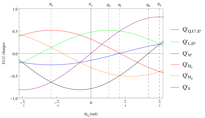
Figure 1: $U(1)^{\prime}$ charges of all the chiral superfields of the UMSSM as function of $\theta_{E_{6}}$.

Figure 1 shows these charges as functions of the mixing angle $\theta_{E_{6}}$. We identify by vertical lines values of $\theta_{E_{6}}$ that generate the well–known $U(1)^{\prime}$ groups denoted by $U(1)^{\prime}_{\psi}$, $U(1)^{\prime}_{N}$, $U(1)^{\prime}_{I}$, $U(1)^{\prime}_{S}$, $U(1)^{\prime}_{\chi}$ and $U(1)^{\prime}_{\eta}$. The black curve in Fig. 1 shows that for $\theta_{E_{6}}=\arctan{\sqrt{15}}$ the $U(1)^{\prime}$ charge of the RH (s)neutrinos vanishes; this corresponds to the $U(1)^{\prime}_{N}$ model of Table 1. This model is not of interest to us, since the $\tilde{\nu}_{R,i}$ are then complete gauge singlets, and do not couple to any potential $s-$channel resonance. Similarly, for $\theta_{E_{6}}=0$, i.e. $U(1)^{\prime}=U(1)^{\prime}_{\chi}$, the charge of $\hat{S}$ vanishes; in that case $s$ cannot be used to break the gauge symmetry, i.e. the field content we have chosen is not sufficient to achieve the complete breaking of the (extended) electroweak gauge symmetry down to $U(1)_{\rm QED}$. All other values of $\theta_{E_{6}}$ are acceptable for us.

The superpotential of the UMSSM contains, besides the MSSM superpotential without $\mu$ term, a term that couples the extra singlet superfield to the two doublet Higgs superfields; this term is always allowed, since it is part of the gauge invariant ${\bf 27}^{3}$ of $E_{6}$. The superpotential also contains Yukawa couplings for the neutrinos. We thus have:

$$\hat{W}=\hat{W}_{MSSM}|_{\mu=0}+\lambda\hat{S}\hat{H}_{u}\cdot\hat{H}_{d}+\hat{N}^{C}{\bf Y_{\nu}}\hat{L}\cdot\hat{H}_{u}\,,$$ (5)

where $\cdot$ stands for the antisymmetric $SU(2)$ invariant product of two doublets. The neutrino Yukawa coupling ${\bf Y_{\nu}}$ is a $3\times 3$ matrix in generation space and $\lambda$ is a dimensionless coupling. Note that for $\theta_{E_{6}}\neq 0$ the $U(1)^{\prime}$ symmetry forbids both bilinear $\hat{N}^{C}_{i}\hat{N}^{C}_{j}$ and trilinear $\hat{S}\hat{N}^{C}_{i}\hat{N}^{C}_{j}$ terms in the superpotential. In this model the neutrinos therefore obtain pure Dirac masses, which means that the Yukawa couplings $Y_{\nu,ij}$ must be of order $10^{-11}$ or less; in our numerical analysis we therefore set ${\bf Y_{\nu}}=0$.

The electroweak and the $U(1)^{\prime}$ gauge symmetries are spontaneously broken when, in the minimum of the scalar potential, the real parts of the doublet and singlet Higgs fields acquire non–zero vacuum expectation values. These fields are expanded as

$$\begin{split}H_{d}^{0}&=\frac{1}{\sqrt{2}}\left(v_{d}+\phi_{d}+i\sigma_{d}\right)\,;\end{split}$$ (6a)

$$\begin{split}H_{u}^{0}&=\frac{1}{\sqrt{2}}\left(v_{u}+\phi_{u}+i\sigma_{u}\right)\,;\end{split}$$ (6b)

$$\begin{split}s&=\frac{1}{\sqrt{2}}\left(v_{s}+\phi_{s}+i\sigma_{s}\right)\,.\end{split}$$ (6c)

We define $\tan{\beta}=\frac{v_{u}}{v_{d}}$ and $v=\sqrt{v_{d}^{2}+v_{u}^{2}}$ exactly as in the MSSM; this describes the breaking of the $SU(2)_{L}\times U(1)_{Y}$ symmetry, and makes subleading contributions to the breaking of $U(1)^{\prime}$. The latter is mostly accomplished by the VEV of $s$. The coupling $\lambda$ in eq.(5) then generates an effective $\mu-$term:

$$\mu_{\rm eff}=\lambda\frac{v_{s}}{\sqrt{2}}\,.$$ (7)

As well known, supersymmetry needs to be broken. We parameterize this by soft breaking terms book :

$$-\mathcal{L}_{SB} =m^{2}_{H_{d}}|H_{d}|^{2}+m^{2}_{H_{u}}|H_{u}|^{2}+m_{S}^{2}|s|^{2}+\tilde{Q}^{\dagger}{\bf m^{2}_{\tilde{Q}}}\tilde{Q}+\tilde{d}_{R}^{\dagger}{\bf m^{2}_{\tilde{D}^{C}}}\tilde{d}_{R}$$

$$+\tilde{u}_{R}^{\dagger}{\bf m^{2}_{\tilde{U}^{C}}}\tilde{u}_{R}+\tilde{L}^{\dagger}{\bf m^{2}_{\tilde{L}}}\tilde{L}+\tilde{e}_{R}^{\dagger}{\bf m^{2}_{\tilde{E}^{C}}}\tilde{e}_{R}+\tilde{\nu}_{R}^{\dagger}{\bf m^{2}_{\tilde{N}^{C}}}\tilde{\nu}_{R}$$

$$+\frac{1}{2}\Big{(}M_{1}\lambda_{\tilde{B}}\lambda_{\tilde{B}}+M_{2}\lambda_{\tilde{W}}\lambda_{\tilde{W}}+M_{3}\lambda_{\tilde{g}}\lambda_{\tilde{g}}+M_{4}\lambda_{\tilde{B}^{\prime}}\lambda_{\tilde{B}^{\prime}}+h.c.\Big{)}$$ (8)

$$+\Big{(}\tilde{u}_{R}^{C}{\bf T_{u}}\tilde{Q}_{L}\cdot H_{u}-\tilde{d}_{R}^{C}{\bf T_{d}}\tilde{Q}_{L}\cdot H_{d}-\tilde{e}_{R}^{C}{\bf T_{e}}\tilde{L}_{L}\cdot H_{d}+T_{\lambda}sH_{u}\cdot H_{d}+\tilde{\nu}_{R}^{C}{\bf T_{\nu}}\tilde{L}_{L}\cdot H_{u}+h.c.\Big{)}\,.$$

Here we have used the notation of SPheno Porod:2003um ; Porod:2011nf . The soft scalar masses and the soft trilinear parameters of the sfermions are again $3\times 3$ matrices in generation space. In the UMSSM, the $B\mu$ term of the MSSM is induced by the $T_{\lambda}$ term after the breaking of the $U(1)^{\prime}$ gauge symmetry.

In the following subsections we discuss those parts of the spectrum in a bit more detail that are important for our calculation. These are the sfermions, in particular sneutrinos; the massive gauge bosons; the Higgs bosons; and the neutralinos. The lightest right–handed sneutrino is assumed to be the LSP, which annihilates chiefly through the exchange of massive gauge and Higgs bosons in the $s-$channel. Requiring the lightest neutralino to be sufficiently heavier than the lightest right–handed sneutrino gives important constraints on the parameter space. The mass matrices in these subsections have been obtained with the help of the computer code SARAH Staub:2008uz ; Staub:2013tta ; Staub:2015kfa ; many of these results can also be found in refs. Belanger:2011rs ; Belanger:2015cra ; Belanger:2017vpq .

2.2 Sfermions

In the UMSSM, the $U(1)^{\prime}$ gauge symmetry induces some new $D-$term contributions to the masses of all sfermions with nonvanishing $U(1)^{\prime}$ charges. These modify the diagonal entries of the MSSM sfermion mass matrices:

$$\Delta_{F}=\frac{1}{2}g^{\prime 2}Q^{\prime}_{F}\Big{(}Q^{\prime}_{H_{d}}v_{d}^{2}+Q^{\prime}_{H_{u}}v_{u}^{2}+Q^{\prime}_{S}v_{s}^{2}\Big{)}\,,$$ (9)

where $g^{\prime}$ is the $U(1)^{\prime}$ gauge coupling and $F\in\{Q,L,D^{C},U^{C},E^{C},N^{C}\}$. LHC searches for $Z^{\prime}$ production in the dilepton channel imply pdg $M^{2}_{Z^{\prime}}\gg M^{2}_{Z}$, and hence $v_{s}^{2}\gg v_{u}^{2},\,v_{d}^{2}$. The first two terms on the right–hand side (RHS) of eq.(9) are therefore essentially negligible. However, due to the contribution $\propto v_{s}^{2}$ these $D-$terms can dominate the sfermion masses. Moreover, depending on the value of $\theta_{E_{6}}$ these terms can be positive or negative. For example, Fig. 1 shows that for $\arctan\sqrt{15}<\theta_{E_{6}}<\frac{\pi}{2}$ all the sfermion masses receive positive corrections, the corrections to the RH sneutrino masses being the smallest ones. In contrast, for $0<\theta_{E_{6}}<\arctan\sqrt{15}$ the $D-$term contribution to the RH sneutrino masses is negative. For $\theta_{E_{6}}<0$ the RH sneutrino masses again receive positive corrections from this $D-$term.

The tree–level sneutrino mass matrix written in the basis $\left(\tilde{\nu}_{L},\tilde{\nu}_{R}\right)$ is

$$\mathcal{M}^{2}_{\tilde{\nu}}=\left(\begin{array}[]{cc}{\bf m}_{\tilde{\nu}_{L}\tilde{\nu}_{L}^{*}}^{2}&-\frac{1}{2}v_{d}v_{s}\lambda{\bf Y_{\nu}^{*}}+\frac{1}{\sqrt{2}}v_{u}{\bf T_{\nu}^{*}}\\ -\frac{1}{2}v_{d}v_{s}\lambda{\bf Y}_{\nu}^{T}+\frac{1}{\sqrt{2}}v_{u}{\bf T}_{\nu}^{T}&{\bf m}_{\tilde{\nu}_{R}\tilde{\nu}_{R}^{*}}^{2}\end{array}\right)\,.$$ (10)

The $3\times 3$ sub–matrices along the diagonal are given by:

$${\bf m}_{\tilde{\nu}_{L}\tilde{\nu}_{L}^{*}}^{2} =\Big{[}\Delta_{L}+\frac{1}{8}\Big{(}g_{1}^{2}+g_{2}^{2}\Big{)}\Big{(}v_{d}^{2}-v_{u}^{2}\Big{)}\Big{]}{\bf 1}+\frac{1}{2}v_{u}^{2}{{\bf Y}_{\nu}^{*}{\bf Y}_{\nu}^{T}}+{\bf m^{2}_{\tilde{L}}}\,;$$ (11a)

$${\bf m}_{\tilde{\nu}_{R}\tilde{\nu}_{R}^{*}}^{2} =\Delta_{N^{C}}{\bf 1}+\frac{1}{2}v_{u}^{2}{{\bf Y}_{\nu}^{T}{\bf Y}_{\nu}^{*}}+{\bf m^{2}_{\tilde{N}^{C}}}\,,$$ (11b)

where $g_{1}$ and $g_{2}$ are the $U(1)_{Y}$ and $SU(2)_{L}$ gauge couplings, respectively. As noted earlier, the neutrino Yukawa couplings have to be very small. We therefore set ${\bf Y_{\nu}}={\bf T_{\nu}}=0$, so that the $6\times 6$ matrix (10) decomposes into two $3\times 3$ matrices. Since all interactions of the $\tilde{\nu}_{R}$ fields are due to $U(1)^{\prime}$ gauge interactions which are the same for all generations, we can without loss of generality assume that the matrix ${\bf m^{2}_{\tilde{N}^{C}}}$ of soft breaking masses is diagonal. The physical masses of the RH sneutrinos are then simply given by $m^{2}_{\tilde{\nu}_{R,i}}=m^{2}_{\tilde{N}^{C}_{i}}+\Delta_{N^{C}}$. Our LSP candidate is the lightest of the three $\tilde{\nu}_{R}$ states, which we call $\tilde{\nu}_{R,1}$.

2.3 Gauge Bosons

The UMSSM contains three neutral gauge bosons, from the $SU(2)_{L},\,U(1)_{Y}$ and $U(1)^{\prime}$, respectively. As in the SM and MSSM, after symmetry breaking one linear combination of the neutral $SU(2)_{L}$ and $U(1)_{Y}$ gauge bosons remains massless; this is the photon. The orthogonal state $Z_{0}$ mixes with the $U(1)^{\prime}$ gauge boson $Z_{0}^{\prime}$ via a $2\times 2$ mass matrix:

$$\mathcal{M}^{2}_{ZZ^{\prime}}=\,\left(\begin{array}[]{cc}M_{Z_{0}}^{2}&\Delta_{Z}\\ \Delta_{Z}&M_{Z_{0}^{\prime}}^{2}\end{array}\right)\,,$$ (12)

with

$$M_{Z_{0}}^{2} = \frac{1}{4}(g_{1}^{2}+g_{2}^{2})v^{2}\,;$$ (13)

$$\Delta_{Z} = \frac{1}{2}g^{\prime}\sqrt{g_{1}^{2}+g_{2}^{2}}\left(Q^{\prime}_{H_{d}}v_{d}^{2}-Q^{\prime}_{H_{u}}v_{u}^{2}\right)\,;$$ (14)

$$M_{Z^{\prime}_{0}}^{2} = g^{\prime 2}\Big{(}Q^{\prime 2}_{H_{d}}v_{d}^{2}+Q^{\prime 2}_{H_{u}}v_{u}^{2}+Q^{\prime 2}_{S}v_{s}^{2}\Big{)}\,.$$ (15)

Recall that $g_{2},\,g_{1}$ and $g^{\prime}$ are the gauge couplings associated to $SU(2)_{L},\,U(1)_{Y}$ and $U(1)^{\prime}$, respectively. The eigenstates $Z$ and $Z^{\prime}$ of this mass matrix can be written as:

$$Z = \cos{\alpha_{ZZ^{\prime}}}Z_{0}+\sin{\alpha_{ZZ^{\prime}}}Z_{0}^{\prime}\,;$$

$$Z^{\prime} = -\sin{\alpha_{ZZ^{\prime}}}Z_{0}+\cos{\alpha_{ZZ^{\prime}}}Z_{0}^{\prime}\,.$$ (16)

The mixing angle $\alpha_{ZZ^{\prime}}$ is given by

$$\sin{2\alpha_{ZZ^{\prime}}}=\frac{2\Delta_{Z}}{M_{Z}^{2}-M_{Z^{\prime}}^{2}}\,.$$ (17)

The masses of the physical states are

$$M_{Z,Z^{\prime}}^{2}=\frac{1}{2}\left[M_{Z_{0}}^{2}+M_{Z^{\prime}_{0}}^{2}\mp\sqrt{\left(M_{Z^{\prime}_{0}}^{2}-M_{Z_{0}}^{2}\right)^{2}+4\Delta_{Z}^{2}}\ \right]\,.$$ (18)

Note that the off–diagonal entry $\Delta_{Z}$ in eq.(12) is of order $v^{2}$. We are interested in $Z^{\prime}$ masses in excess of $10$ TeV, which implies $v_{s}^{2}\gg v^{2}$. The mixing angle $\alpha_{ZZ^{\prime}}$ is ${\cal O}(M_{Z}^{2}/M^{2}_{Z^{\prime}})$, which is automatically below current limits pdg if $M_{Z^{\prime}}\geq 10$ TeV. Moreover, mass mixing increases the mass of the physical $Z^{\prime}$ boson only by a term of order $M^{4}_{Z}/M^{3}_{Z^{\prime}}$, which is less than $0.1$ MeV for $M_{Z^{\prime}}\geq 10$ TeV. To excellent approximation we can therefore identify the physical $Z^{\prime}$ mass with $M_{Z^{\prime}_{0}}$ given in eq.(15), with the last term $\propto v_{s}^{2}$ being the by far dominant one.

Recall from the discussion of the previous subsection that the mass of the right–handed sneutrinos can get a large positive contribution from the $U(1)^{\prime}$ $D-$term for some range of $\theta_{E_{6}}$. In fact, from eqs.(9) and (15) together with the charges listed in Table 1 we find that this $D-$term contribution exceeds $(M_{Z^{\prime}}/2)^{2}$ if

$$-\sqrt{15}<\tan\theta_{E_{6}}<0\,.$$ (19)

For this range of $\theta_{E_{6}}$ one therefore needs a negative squared soft breaking contribution $m^{2}_{\tilde{N}^{C}_{1}}$ in order to obtain $M_{\tilde{\nu}_{R,1}}\simeq M_{Z^{\prime}}/2$.

Note that we neglect kinetic $Z-Z^{\prime}$ mixing Kalinowski:2008iq ; Belanger:2017vpq . In the present context this is a loop effect caused by the mass splitting of members of the ${\bf 27}$ of $E_{6}$. This induces small changes of the couplings of the physical $Z^{\prime}$ boson, which have little effect on our result; besides, this loop effect should be treated on the same footing as other one–loop corrections.

2.4 The Higgs Sector

The Higgs sector of the UMSSM contains two complex $SU(2)_{L}$ doublets $H_{u,d}$ and the complex singlet $s$. Four degrees of freedom get “eaten” by the longitudinal components of $W^{\pm},\,Z$ and $Z^{\prime}$. This leaves three neutral CP–even Higgs bosons $h_{i},\,i\in\{1,2,3\}$, one CP-odd Higgs boson $A$ and two charged Higgs bosons $H^{\pm}$ as physical states. After solving the minimization conditions of the scalar potential for the soft breaking masses of the Higgs fields, the symmetric $3\times 3$ mass matrix for the neutral CP–even states in the basis $(\phi_{d},\phi_{u},\phi_{s})$ has the following tree–level elements:

$$\left(\mathcal{M}_{+}^{0}\right)_{\phi_{d}\phi_{d}} =\Big{[}\frac{g_{1}^{2}+g_{2}^{2}}{4}+(Q^{\prime}_{H_{d}})^{2}g^{\prime 2}\Big{]}v_{d}^{2}+\frac{T_{\lambda}v_{s}v_{u}}{\sqrt{2}v_{d}}\,;$$ (20a)

$$\left(\mathcal{M}_{+}^{0}\right)_{\phi_{d}\phi_{u}} =-\Big{[}\frac{g_{1}^{2}+g_{2}^{2}}{4}-g^{\prime 2}Q^{\prime}_{H_{d}}Q^{\prime}_{H_{u}}-\lambda^{2}\Big{]}v_{d}v_{u}-\frac{T_{\lambda}v_{s}}{\sqrt{2}}\,;$$ (20b)

$$\left(\mathcal{M}_{+}^{0}\right)_{\phi_{d}\phi_{s}} =\Big{[}g^{\prime 2}Q^{\prime}_{H_{d}}Q^{\prime}_{S}+\lambda^{2}\Big{]}v_{d}v_{s}-\frac{T_{\lambda}v_{u}}{\sqrt{2}}\,;$$ (20c)

$$\left(\mathcal{M}_{+}^{0}\right)_{\phi_{u}\phi_{u}} =\Big{[}\frac{g_{1}^{2}+g_{2}^{2}}{4}+(Q^{\prime}_{H_{u}})^{2}g^{\prime 2}\Big{]}v_{u}^{2}+\frac{T_{\lambda}v_{s}v_{d}}{\sqrt{2}v_{u}}\,;$$ (20d)

$$\left(\mathcal{M}_{+}^{0}\right)_{\phi_{u}\phi_{s}} =\Big{[}g^{\prime 2}Q^{\prime}_{H_{u}}Q^{\prime}_{S}+\lambda^{2}\Big{]}v_{u}v_{s}-\frac{T_{\lambda}v_{d}}{\sqrt{2}}\,;$$ (20e)

$$\left(\mathcal{M}_{+}^{0}\right)_{\phi_{s}\phi_{s}} =g^{\prime 2}(Q^{\prime}_{S})^{2}v_{s}^{2}+\frac{T_{\lambda}v_{d}v_{u}}{\sqrt{2}v_{s}}\,.$$ (20f)

In general the eigenstates and eigenvalues of this mass matrix have to be obtained numerically. We denote the mass eigenstates by $h_{1},\,h_{2},\,h_{3}$, ordered in mass.

The tree level mass of the single physical neutral CP–odd state is

$$M_{A}^{2}|_{\text{tree}}=\frac{\sqrt{2}T_{\lambda}}{\sin{2\beta}}v_{s}\left(1+\frac{v^{2}}{4v_{s}^{2}}\sin^{2}{2\beta}\right)\,.$$ (21)

In our sign convention, $\tan\beta$ and $v_{s}$ are positive in the minimum of the potential; eq.(21) then implies that $T_{\lambda}$ must also be positive. As in the MSSM $M_{A}^{2}$ differs from the squared mass of the physical charged Higgs boson only by terms of order $v^{2}$:

$$M_{H^{+}}^{2}|_{\text{tree}}=M_{W^{+}}^{2}+\frac{\sqrt{2}T_{\lambda}}{\sin{2\beta}}v_{s}-\frac{\lambda^{2}}{2}v^{2}\,.$$ (22)

Both $A$ and $H^{\pm}$ are constructed from the components of $H_{u}$ and $H_{d}$, without any admixture of $s$.

Recall that we are interested in the limit $v_{s}\gg v$. Eqs.(20) show that the entries mixing the $SU(2)_{L}$ singlet with the doublets are of order $v_{s}v$ or $T_{\lambda}v$, whereas the diagonal mass of the singlet is of order $v_{s}^{2}$. The mixing between singlet and doublet states is therefore small. Moreover, we will work in the MSSM–like decoupling limit $M_{A}^{2}\gg M_{Z}^{2}$, which ensures that the lightest neutral CP–even Higgs boson has couplings close to those of the SM Higgs. Its mass can then approximately be written as King:2005jy ; Belanger:2017vpq :

$$M_{h_{1}}^{2}|_{\text{tree}} \simeq \frac{1}{4}(g_{1}^{2}+g_{2}^{2})v^{2}\cos^{2}2\beta+\frac{1}{2}\lambda^{2}v^{2}\sin^{2}2\beta+g^{\prime 2}v^{2}\left(Q^{\prime}_{H_{d}}\cos^{2}\beta+Q^{\prime}_{H_{u}}\sin^{2}\beta\right)^{2}$$ (23)

$$- \frac{v^{2}}{g^{\prime 2}(Q^{\prime}_{S})^{2}}\Big{[}\lambda^{2}-\frac{T_{\lambda}\sin^{2}2\beta}{\sqrt{2}v_{s}}+g^{\prime 2}Q^{\prime}_{S}\left(Q^{\prime}_{H_{d}}\cos^{2}\beta+Q^{\prime}_{H_{u}}\sin^{2}\beta\right)\Big{]}^{2}\,.$$

The first term on the RHS is as in the MSSM. The second term is an $F-$term contribution that also appears in the NMSSM, while the third term is due to the $U(1)^{\prime}$ $D-$ term. These terms are positive. The second line is due to mixing between singlet and doublet states; note that this mixing always reduces the mass of the lighter eigenstate, but increases the mass of the heaviest state $h_{3}$. As well known, the mass of $h_{1}$ also receives sizable loop corrections, in particular from the top–stop sector Okada:1990vk ; Haber:1990aw ; we will briefly discuss them below when we describe our numerical procedures.

As noted above, in the limit $v_{s}\gg v$ the mixing between singlet and doublet states can to first approximation be neglected. Here we chose the heaviest state to be (mostly) singlet. From the last eq.(20) and eq.(15) we derive the important result

$$M^{2}_{Z^{\prime}}|_{\text{tree}}\simeq M_{h_{3}}^{2}|_{\text{tree}}+{\cal O}(v^{2})\,.$$ (24)

Here we have assumed $|T_{\lambda}|\leq v_{s}$ because for larger values of $|T_{\lambda}|$ the mass of the heavy doublet Higgs can exceed the mass of the singlet state. As we will see, in the region of parameter space that minimizes the $\tilde{\nu}_{R,1}$ relic density we need $M_{A}<M_{\tilde{\nu}_{R,1}}$.

Eq.(24) leads to an $h_{3}-Z^{\prime}$ mass splitting of order $M^{2}_{Z}/M_{Z^{\prime}}$, which is below $1$ GeV for $M_{Z^{\prime}}>10$ TeV. Loop corrections induce significantly larger mass splittings, with $M_{Z^{\prime}}>M_{h_{3}}$; however, the splitting still amounts to less than $1\%$ in the relevant region of parameter space, which is well below the typical kinetic energy of WIMPs in the epoch around their decoupling from the thermal bath. We thus arrive at the important result that $M_{\tilde{\nu}_{R,1}}\simeq M_{Z^{\prime}}$ automatically implies $M_{\tilde{\nu}_{R,1}}\simeq M_{h_{3}}$ in our set–up, so that $\tilde{\nu}_{R,1}$ annihilation is enhanced by two nearby resonances.

2.5 Neutralinos

The neutralino sector is formed by the fermionic components of the neutral vector and Higgs supermultiplets. So, in addition to the neutralino sector of the MSSM, the UMSSM has another gaugino state associated with the $U(1)^{\prime}$ gauge symmetry and a singlino state that comes from the extra scalar supermultiplet $\hat{S}$. The neutralino mass matrix written in the basis $\left(\lambda_{\tilde{B}},\tilde{W}^{0},\tilde{H}_{d}^{0},\tilde{H}_{u}^{0},\tilde{S},\lambda_{\tilde{B}^{\prime}}\right)$ is:

$$\mathcal{M}_{\tilde{\chi}^{0}}=\left(\begin{array}[]{cccccc}M_{1}&0&-\frac{1}{2}g_{1}v_{d}&\frac{1}{2}g_{1}v_{u}&0&0\\ 0&M_{2}&\frac{1}{2}g_{2}v_{d}&-\frac{1}{2}g_{2}v_{u}&0&0\\ -\frac{1}{2}g_{1}v_{d}&\frac{1}{2}g_{2}v_{d}&0&-\mu_{\rm eff}&-\frac{1}{\sqrt{2}}v_{u}\lambda&g^{\prime}Q^{\prime}_{H_{d}}v_{d}\\ \frac{1}{2}g_{1}v_{u}&-\frac{1}{2}g_{2}v_{u}&-\mu_{\rm eff}&0&-\frac{1}{\sqrt{2}}v_{d}\lambda&g^{\prime}Q^{\prime}_{H_{u}}v_{u}\\ 0&0&-\frac{1}{\sqrt{2}}v_{u}\lambda&-\frac{1}{\sqrt{2}}v_{d}\lambda&0&g^{\prime}Q^{\prime}_{S}v_{s}\\ 0&0&g^{\prime}Q^{\prime}_{H_{d}}v_{d}&g^{\prime}Q^{\prime}_{H_{u}}v_{u}&g^{\prime}Q^{\prime}_{S}v_{s}&M_{4}\end{array}\right)\,.$$ (25)

This matrix is diagonalized by a unitary 6 $\times$ 6 matrix $N$ which gives the mass eigenstates (in order of increasing mass) $\tilde{\chi}^{0}_{1},\,\tilde{\chi}^{0}_{2},\,\tilde{\chi}^{0}_{3},\tilde{\chi}^{0}_{4},\,\tilde{\chi}^{0}_{5},\,\tilde{\chi}^{0}_{6}$ as a linear combinations of the current eigenstates. We have ignored a possible (gauge invariant) mixed $\tilde{B}\tilde{B}^{\prime}$ mass term Suematsu:1997qt ; Suematsu:1997au .

Note that the singlet higgsino (singlino for short) $\tilde{S}$ and the $U(1)^{\prime}$ gaugino $\tilde{B}^{\prime}$ mix strongly, through an entry of order $v_{s}$. On the other hand, these two new states mix with the MSSM only through entries of order $v$. Therefore the eigenvalues of the lower–right $2\times 2$ submatrix in eq.(25) are to good approximation also eigenvalues of the entire neutralino mass matrix. Note that the smaller of these two eigenvalues decreases with increasing $M_{4}$. Requiring this eigenvalue to be larger than $M_{\tilde{\nu}_{R,1}}\simeq M_{Z^{\prime}}/2$ therefore implies

$$|M_{4}|<\frac{3}{2}M_{Z^{\prime}}\,.$$ (26)

Moreover, the smallest mass of the MSSM–like states should also be larger than $M_{Z^{\prime}}/2$, which implies

$$|M_{1}|>\frac{1}{2}M_{Z^{\prime}};\ |M_{2}|>\frac{1}{2}M_{Z^{\prime}};\ |\lambda|>\frac{1}{\sqrt{2}}|Q_{S}g^{\prime}|\,.$$ (27)

We have used eqs.(7) and (15) in the derivation of the last inequality.

We finally note that the chargino sector of the UMSSM is identical to that of the MSSM, with $\mu\rightarrow\mu_{\rm eff}$.

3 Minimizing the Relic Abundance of the Right-Handed Sneutrino

As described in the Introduction, we want to find the upper bound on the mass of the lightest RH sneutrino $\tilde{\nu}_{R,1}$ from the requirement that it makes a good thermal WIMP in standard cosmology. As well known kt , under the stated assumptions the WIMP relic density is essentially inversely proportional to the thermal average of its annihilation cross section into lighter particles; these can be SM particles or Higgs bosons of the extended sector. The upper bound on $M_{\tilde{\nu}_{R,1}}$ will therefore be saturated for combinations of parameters that maximize the thermally averaged $\tilde{\nu}_{R,1}\tilde{\nu}_{R,1}^{*}$ annihilation cross section.

All relevant couplings of the RH sneutrinos are proportional to the $U(1)^{\prime}$ gauge coupling $g^{\prime}$. In particular, two RH sneutrinos can annihilate into two neutrinos through exchange of a $U(1)^{\prime}$ gaugino. This, and similar reactions where one or both particles in the initial and final state are replaced by antiparticles, are typical electroweak $2\rightarrow 2$ reactions without enhancement factors. They will therefore not allow RH sneutrino masses in the multi–TeV range.

In contrast, $\tilde{\nu}_{R,1}\tilde{\nu}_{R,1}^{*}$ annihilation through $Z^{\prime}$ and scalar $h_{3}$ exchange can be resonantly enhanced if $M_{\tilde{\nu}_{R,1}}\simeq M_{Z^{\prime}}/2$; recall that $M_{h_{3}}\simeq M_{Z^{\prime}}$ is automatic in our set–up, if $h_{3}$ is mostly an SM singlet, as we assume. Note that the $Z^{\prime}$ exchange can only contribute if the sneutrinos are in a $P-$wave. This suppresses the thermal average of the cross section by a factor $\geq 7$. For comparable couplings, $h_{3}$ exchange, which is depicted in Fig. 2, is therefore more important.

Figure 2: Main annihilation process for the annihilation of RH sneutrinos. The final state can contain both physical Higgs particles and the longitudinal components of the weak $W$ and $Z$ gauge bosons, which are equivalent to the corresponding would–be Goldstone modes.

In the $h_{3}$ resonance region the annihilation cross section scales like

$$\sigma_{\rm ann}\propto\frac{(Q^{\prime}_{N^{C}})^{2}}{M^{2}_{\tilde{\nu}_{R,1}}}\,.$$ (28)

Since the $h_{3}\tilde{\nu}_{R,1}\tilde{\nu}_{R,1}^{*}$ coupling, denoted by $C_{1}$ in Fig. 2, originates from the $U(1)^{\prime}$ $D-$term, it is proportional to the product of $S$ and $N^{C}$ charges:

$$\left|C_{1}\right|\simeq g^{\prime 2}\left|Q^{\prime}_{N^{C}}Q^{\prime}_{S}v_{s}\right|\,.$$ (29)

These charges are determined uniquely once the angle $\theta_{E_{6}}$ has been fixed. The denominator in eq.(28) results from dimensional arguments, using the fact that there is essentially only one relevant mass scale once the resonance condition has been imposed.

Note that near the resonance the annihilation cross section is effectively only ${\cal O}(\alpha^{\prime})$, not ${\cal O}(\alpha^{\prime 2})$, where $\alpha^{\prime}=g^{\prime 2}/(4\pi)$. The $\tilde{\nu}_{R,1}\tilde{\nu}_{R,1}^{*}$ annihilation cross section is then larger than typical co–annihilation cross sections, if the latter are not resonantly enhanced. Even co–annihilation with a superparticle that can also annihilate resonantly (e.g., a higgsino–like neutralino) will not increase the effective annihilation cross section, but will increase the effective number of degrees of freedom per dark matter particle $g_{\chi}$. As a result, we find that co–annihilation reduces the upper bound on $M_{\tilde{\nu}_{R,1}}$. For example, if all three RH sneutrinos have the same mass, the upper bound on this mass decreases by a factor of $\sqrt{3}$, since the annihilation cross section has to be increased by a factor of $3$ in order to compensate the increase of $g_{\chi}$. We therefore require that the lightest neutralino is at least $20\%$ heavier than $\tilde{\nu}_{R,1}$.

As noted earlier, the initial–state coupling $C_{1}$ in Fig. 2 is essentially fixed by $\theta_{E_{6}}$. The upper bound on $M_{\tilde{\nu}_{R,1}}$ for given $\theta_{E_{6}}$ can therefore be found by optimizing the final state couplings. We find that the relic density is minimized if the effective final state coupling $C_{2}$, defined more precisely below, is of the same order as $C_{1}$. This can be understood as follows. For much larger values of $C_{2}$ the width of $h_{3}$ increases, which reduces the cross section. On the other hand, since the peak of the thermally averaged cross section is reached for $M_{\tilde{\nu}_{R,1}}$ slightly below $M_{h_{3}}/2$ Griest:1990kh , $h_{3}\rightarrow\tilde{\nu}_{R,1}\tilde{\nu}_{R,1}^{*}$ decays are allowed, and dominate the total $h_{3}$ width if $C_{2}\ll C_{1}$; in this case increasing $C_{2}$ will clearly increase the cross section, i.e. reduce the relic density.

The only sizable couplings of the singlet–like Higgs state $h_{3}$ to particles with even $R-$parity (i.e., to particles possibly lighter than the LSP $\tilde{\nu}_{R,1}$) are to members of the Higgs doublets. $h_{3}$ couples to $H_{u}$ and $H_{d}$ through the $U(1)^{\prime}$ $D-$term, with contributions $\propto g^{\prime 2}Q^{\prime}_{S}Q^{\prime}_{H_{u},H_{d}}v_{s}$; through $F-$terms associated to the coupling $\lambda$, with contributions $\propto\lambda^{2}v_{s}$; and through a trilinear soft breaking term, with contributions $\propto T_{\lambda}$. In the decoupling limit $M_{A}^{2}\gg M_{Z}^{2}$ the relevant couplings are given by:

$$C_{h_{3}H^{+}H^{-}}\simeq C_{h_{3}h_{2}h_{2}}\simeq C_{h_{3}AA}\simeq-i \Big{[} g^{\prime 2}\left(\cos^{2}\beta Q^{\prime}_{H_{u}}+\sin^{2}\beta Q^{\prime}_{H_{d}}\right)Q^{\prime}_{S}v_{s}$$ (30)

$$+ v_{s}\lambda^{2}+\frac{\sin(2\beta)}{\sqrt{2}}T_{\lambda}\Big{]}\,;$$

$$C_{h_{3}G^{+}G^{-}}\simeq C_{h_{3}h_{1}h_{1}}\simeq C_{h_{3}G^{0}G^{0}}\simeq-i \Big{[} g^{\prime 2}\left(\sin^{2}\beta Q^{\prime}_{H_{u}}+\cos^{2}\beta Q^{\prime}_{H_{d}}\right)Q^{\prime}_{S}v_{s}$$ (31)

$$+ v_{s}\lambda^{2}-\frac{\sin(2\beta)}{\sqrt{2}}T_{\lambda}\Big{]}\,;$$

$$C_{h_{3}H^{+}G^{-}}\simeq C_{h_{3}h_{2}h_{1}}\simeq C_{h_{3}AG^{0}}\simeq-i \Big{[} g^{\prime 2}\frac{\sin(2\beta)}{2}\left(Q^{\prime}_{H_{u}}-Q^{\prime}_{H_{d}}\right)Q^{\prime}_{S}v_{s}$$ (32)

$$- \frac{\cos(2\beta)}{\sqrt{2}}T_{\lambda}\Big{]}\,.$$

Since $M_{h_{3}}\gg v$, at scale $M_{h_{3}}$ $SU(2)_{L}$ is effectively unbroken. The couplings of $h_{3}$ to two members of the heavy doublet containing the physical states $H^{\pm},h_{2}$ and $A$ therefore are all the same, see eq.(30), as are the couplings to the light doublet containing $h_{1}$ and the would–be Goldstone modes $G^{0}$ and $G^{\pm}$, see eq.(31); finally, eq.(32) describes the common coupling to one member of the heavy doublet and one member of the light doublet. Of course, the would–be Goldstone modes are not physical particles; however, again since $M_{h_{3}}\gg v$ the production of physical longitudinal gauge bosons can to very good approximation be described as production of the corresponding Goldstone states. This is the celebrated equivalence theorem Cornwall:1974km .

We find numerically that the $\tilde{\nu}_{R,1}$ relic density is minimized when $h_{3}$ decays into two members of the heavy Higgs doublet are allowed. From eqs.(21) and (22) we see that this requires

$$\frac{\sqrt{2}T_{\lambda}v_{s}}{\sin{2\beta}}<\frac{1}{4}g^{\prime 2}\left(Q^{\prime}_{S}\right)^{2}v_{s}^{2}\quad\quad\quad\Rightarrow\quad\quad\quad T_{\lambda}<\frac{g^{\prime 2}\left(Q^{\prime}_{S}\right)^{2}\sin{2\beta}}{4\sqrt{2}}v_{s}\,.$$ (33)

This implies that the singlet–like state is indeed the heaviest physical Higgs boson.

We can now define an effective final–state coupling $C_{2}$ for the diagram shown in Fig. 2:

$$C_{2}=\sqrt{2\left|C_{h_{3}h_{2}h_{2}}\right|^{2}\sqrt{1-\frac{4M_{h_{2}}^{2}}{M_{h_{3}}^{2}}}+2\left|C_{h_{3}h_{1}h_{1}}\right|^{2}+4\left|C_{h_{3}h_{2}h_{1}}\right|^{2}\left(1-\frac{M_{h_{2}}^{2}}{M_{h_{3}}^{2}}\right)}\,.$$ (34)

Here we have included the kinematic factors into the effective coupling, using the same mass $M_{h_{2}}$ for all members of the heavy Higgs doublet and ignoring $M_{h_{1}},M_{W}$ and $M_{Z}$, which are much smaller than $M_{h_{3}}$. The numerical coefficients originate from summing over final states: $H^{+}H^{-},\,AA$ and $h_{2}h_{2}$ for the first term, where the last two final states get a factor $1/2$ for identical final state particles; $G^{+}G^{-},\,G^{0}G^{0}$ and $h_{1}h_{1}$ for the second term, again with factor $1/2$ in front of the second and third contribution; and $G^{+}H^{-},\,G^{-}H^{+},\,G^{0}A$ and $h_{1}h_{2}$ for the third term.

Since the contribution from $h_{3}$ exchange is accessible from an $S-$wave initial state, it peaks for DM mass very close to $M_{h_{3}}/2$ where one needs quite small velocity to get exactly to the pole $s=M_{h_{3}}^{2}$; at such a small velocity, the $Z^{\prime}$ exchange contribution, which can only be accessed from a $P-$wave initial state, is quite suppressed. As a consequence, near the peak of the thermally averaged total cross section the $h_{3}$ exchange processes always contributes more than $90\%$ to the total, whereas the $Z^{\prime}$ exchange contribution shrinks as we approach the peak. The latter reaches its maximum at a larger difference between $M_{Z^{\prime}}$ and $2M_{\tilde{\nu}_{R,1}}$, but its contribution exceeds $10\%$ of the total only if $2M_{\tilde{\nu}_{R,1}}$ is at least $3\%$ below $M_{Z^{\prime}}$, or else above the resonance. Note also that the annihilation into pairs of SM fermions via $Z^{\prime}$ exchange is completely determined by $\theta_{E_{6}}$. In principle we could contemplate annihilation into exotic fermions, members of $\mathbf{27}$ of $E_{6}$ that are required for anomaly cancellation, as noted in Sec. 2.1. However, the contribution from the SM fermions already sums to an effective final state coupling which is considerably larger than the initial state coupling; this helps to explain why the $Z^{\prime}$ contribution is always subdominant. Adding additional final states therefore reduces the $Z^{\prime}$ exchange contribution to the $\tilde{\nu}_{R,1}$ annihilation cross section even further. This justifies our assumption that the exotic fermions are too heavy to affect the calculation of the $\tilde{\nu}_{R,1}$ relic density.

Finally, all other processes of the model contribute at most $1\%$ to the thermally averaged total cross section in the resonance region. This shows that the parameters that describe the rest of the spectrum are irrelevant to our calculation, as long as $\tilde{\nu}_{R,1}$ is the LSP and sufficiently separated in mass from the other superparticles to avoid co–annihilation. These parameters were therefore kept fixed in the numerical results presented below.

4 Numerical Results

We are now ready to present numerical results. We will first describe our procedure. Then we discuss two choices for $\theta_{E_{6}}$, i.e. for the $U(1)^{\prime}$ charges, before generalizing to the entire range of possible values of this mixing angle.

4.1 Procedure

We have used the Mathematica package SARAH Staub:2008uz ; Staub:2013tta ; Staub:2015kfa to generate routines for the precise numerical calculation of the spectrum with SPheno Porod:2003um ; Porod:2011nf . This code calculates by default the pole masses of all supersymmetric particles and their corresponding mixing matrices at the full one–loop level in the $\overline{{\rm DR}}$ scheme. SPheno also includes in its calculation all important two–loop corrections to the masses of neutral Higgs bosons Goodsell:2014bna ; Goodsell:2015ira ; Braathen:2017izn . The dark matter relic density and the dark matter nucleon scattering cross section relevant for direct detection experiments are computed with micrOMEGAS-4.2.5 Belanger:2014vza . The mass spectrum generated by SPheno is passed to micrOMEGAS-4.2.5 through the SLHA+ functionality Belanger:2010st of CalcHep Pukhov:2004ca ; Belyaev:2012qa . The numerical scans were performed by combining the different codes using the Mathematica tool SSP Staub:2011dp for which SARAH already writes an input template.

SARAH can generate two different types of templates that can be used as input files for SPheno. One is the high scale input, where the gauge couplings and the soft SUSY breaking parameters are unified at a certain GUT scale and their renormalization group (RG) evolution between the electroweak, SUSY breaking and GUT scale is included. The other one is the low scale input where the gauge couplings, VEVs, superpotential and soft SUSY breaking parameters of the model are all free input parameters that are given at a specific renormalization scale near the sparticle masses, in which case no RG running to the GUT scale is needed. In this template the SM gauge couplings are given at the electroweak scale and evolve to the SUSY scale through their RGEs. The dark matter phenomenology of a model in the WIMP context is usually well studied at low energies; moreover, acceptable low energy phenomenology for both the $U(1)_{\psi}$ and the $U(1)_{\eta}$ model in the limit where the singlet Higgs decouples works much better with nonuniversal boundary conditions Langacker:1998tc . Finally, a bound that is valid for general low–scale values of the relevant parameters will also hold (but can perhaps not be saturated) in constrained scenarios.

In our work we therefore define the relevant free parameters of the UMSSM directly at the SUSY mass scale, which is defined as the geometric mean of the two stop masses. We created new model files for different versions of the UMSSM to be used in SARAH and SPheno where all the $U(1)^{\prime}$ charges are written in terms of the $U(1)$ mixing angle $\theta_{E_{6}}$ using eq.(3).

Our goal is to find the upper bound on the mass of the lightest RH sneutrino, and therefore on $M_{Z^{\prime}}\simeq M_{h_{3}}$. We argued in Sec. 3 that co–annihilation would weaken the bound. We therefore have to make sure that all other superparticles are sufficiently heavy so that they do not play a role in the calculation in the relic density. The precise values of their masses are then irrelevant to us. We therefore fix the soft mass parameters of the gauginos and sfermions to certain values well above $M_{\tilde{\nu}_{R,1}}$; recall from eq.(26) that this implies an upper bound on the mass $M_{4}$ of the $U(1)^{\prime}$ gaugino. As noted in Sec. 2 we set ${\bf Y_{\nu}}=0$, since the small values of the neutrino masses force them to be negligible for the calculation of the relic density. We also set most of the scalar trilinear couplings to zero, except the top trilinear coupling $T_{t}$ which we use together with $\tan\beta$ and $M_{3}$ to keep the SM Higgs mass in the range $125\pm 3$ GeV, where the uncertainty is dominated by the theory error Carena:2013ytb . Since we are interested in superparticle masses in excess of $10$ TeV, the correct value of $M_{h_{1}}$ can be obtained with a relatively small value of $\tan\beta$, which we also fix.

As already noted in the previous Section, all relevant interactions of $\tilde{\nu}_{R,1}$ scale (either linearly or quadratically) with the $U(1)^{\prime}$ gauge coupling $g^{\prime}$. Since our set–up is inspired by gauge unification, we set this coupling equal to the $U(1)_{Y}$ coupling in GUT normalization, i.e.

$$g^{\prime}=\sqrt{\frac{5}{3}}g_{1}\,.$$ (35)

Note also that the charges in Table 1 are normalized such that $\sum\left(Q^{\prime}_{\psi}\right)^{2}=\sum\left(Q^{\prime}_{\chi}\right)^{2}=\frac{3}{5}\sum Y^{2}$, where the sum runs over a complete $\mathbf{27}-$dimensional representation of $E_{6}$ London:1986dk . We will later comment on how the upper bound on $M_{\tilde{\nu}_{R,1}}$ changes when $g^{\prime}$ is varied.

Recalling that we work in a basis where the matrix ${\mathbf{m}}^{2}_{\tilde{N}^{C}}$ is diagonal, with $m^{2}_{\tilde{N}^{C},11}$ being its smallest element, the remaining relevant free parameters are thus:

$$m^{2}_{\tilde{N}^{C},11},\quad v_{s},\quad\lambda,\quad T_{\lambda}\quad\text{and}\quad\theta_{E_{6}}\,.$$ (36)

All these parameters are related to the extended sector that the UMSSM has in addition to the MSSM. Since the mixing angle $\theta_{E_{6}}$ defines the $U(1)^{\prime}$ gauge group, we want to determine the upper bound on the mass of the lightest RH sneutrino as a function of $\theta_{E_{6}}$. We will see below that this will also allow to derive the absolute upper bound, valid for all versions of the UMSSM.

From the discussion of the previous Section we know that the first two of the parameters listed in (36) are strongly correlated by the requirement that $M_{\tilde{\nu}_{R,1}}$ is close to $M_{Z^{\prime}}/2$. More precisely, the minimal relic density is found if the RH sneutrino mass is very roughly one $h_{3}$ decay width below the nominal pole position, the exact distance depending on the couplings $C_{1}$ and $C_{2}$; this shift from the pole position is due to the finite kinetic energy of the sneutrinos at temperatures around the decoupling temperature Griest:1990kh .

The parameters $\lambda$ and $T_{\lambda}$ have to satisfy some bounds. First, requiring the mass of the $SU(2)_{L}$ higgsinos to be at least $20\%$ larger than $M_{Z^{\prime}}/2$ leads to the lower bound

$$\lambda>0.85g^{\prime}|Q^{\prime}_{S}|\,,$$ (37)

where we have used eqs.(7) and (15). Moreover, $T_{\lambda}$ has to satisfy the upper bound (33), so that pairs of the heavy $SU(2)_{L}$ doublet Higgs bosons can be produced in $\tilde{\nu}_{R,1}$ annihilation with $M_{\tilde{\nu}_{R,1}}\simeq M_{Z^{\prime}}/2$. Having fixed $\tan\beta$ and $T_{\lambda}$, the effective final state coupling $C_{2}$ defined in eq.(34) depends only on $\lambda$, which is constrained by eq.(37); fortunately this still leaves us enough freedom to vary $C_{2}$ over a sufficient range.

The bound on the lightest RH sneutrino mass for a given value of $\theta_{E_{6}}$ can then be obtained as follows. We start by choosing some value of $M_{h_{3}}\simeq M_{Z^{\prime}}$ in the tens of TeV range. Note that this fixes the coupling $C_{1}$, since we have already fixed $g^{\prime}$ and $\theta_{E_{6}}$ and hence the charge $Q^{\prime}_{N^{C}}$. We then minimize the relic density for that value of $M_{h_{3}}$ by varying the soft–breaking contribution to the sneutrino mass and $\lambda$; as noted in Sec. 3, the minimum is reached when the physical RH sneutrino mass is just slightly below $M_{Z^{\prime}}/2$, and $C_{2}$ is close to the initial state coupling $C_{1}$ of eq.(29). If the resulting relic density $(\Omega h^{2})_{1}$ is very close to the measured value of eq.(1), we have found the upper bound on $M_{Z^{\prime}}$ and hence on $M_{\tilde{\nu}_{R,1}}$. Otherwise, we change the value of $M_{h_{3}}$ by the factor $\sqrt{0.12/(\Omega h^{2})_{1}}$, and repeat the procedure. Since the minimal relic density to good approximation scales like $M_{h_{3}}^{2}$, see eq.(28), this algorithm converges rather quickly.

4.2 The $U(1)_{\psi}$ Model

We illustrate our procedure first for $U(1)^{\prime}=U(1)_{\psi}$, where the $U(1)^{\prime}$ charge of the RH sneutrinos is relatively small (in fact, the same as for all SM (s)fermions). We choose the SUSY breaking scale to be 18 TeV and we fix $\tan{\beta}=1.0$, $M_{3}=18$ TeV, and ${\bf m^{2}_{\tilde{Q}}}={\bf m^{2}_{\tilde{U}^{C}}}={\bf m^{2}_{\tilde{D}^{C}}}=2\times 10^{8}$ GeV${}^{2}\cdot{\bf 1}$, ${\bf m^{2}_{\tilde{L}}}={\bf m^{2}_{\tilde{E}^{C}}}=2.25\times 10^{8}$ GeV${}^{2}\cdot{\bf 1}$, $\left(m^{2}_{\tilde{N}^{C}}\right)_{22}=2.2\times 10^{8}$ GeV², $\left(m^{2}_{\tilde{N}^{C}}\right)_{33}=2.3\times 10^{8}$ GeV². To keep $M_{h_{1}}$ close to 125 GeV, the top trilinear coupling took values in the following range ${T_{u,33}}=[-55,-33]$ TeV; recall that the physical squared sfermion masses also receive $D-$term contributions, which amount to $M^{2}_{Z^{\prime}}/8$ in this model.

In this model the two Higgs doublets have the same $U(1)^{\prime}$ charge, and the product $Q^{\prime}_{H_{u}}Q^{\prime}_{S}$ is negative. As a result, the $\lambda^{2}$ and the $g^{\prime 2}$ terms in the diagonal couplings given in eqs.(30) and (31) tend to cancel, while the contribution $\propto g^{\prime 2}$ to the off–diagonal couplings given in eq.(32) vanishes. The contributions involving these off–diagonal couplings are therefore subdominant. The largest contribution usually comes from final states involving two heavy $SU(2)_{L}$ doublet Higgs bosons, but the contributions from two light states (including the longitudinal modes of the gauge bosons) are not much smaller. Moreover, due to this cancellation we need relatively large values of $\lambda$; the numerical results shown below have been obtained by varying it in the range from $0.32$ to $0.46$.

Figure 3a depicts the relic abundance of the RH sneutrino as a function of $M_{\tilde{\nu}_{R,1}}$ for different values of the mass of the singlet Higgs boson. All the curves show a pronounced minimum when $M_{\tilde{\nu}_{R,1}}$ is very close to but below $M_{h_{3}}/2$. The blue and the green curves are for $v_{s}=59$ TeV and thus have the same coupling $C_{1}$ and (approximately) the same mass of the singlet Higgs, but the blue curve has a smaller value of $C_{2}$. This reduces the width of $h_{3}$ as well as the annihilation cross section away from the resonance, and therefore leads to a narrower minimum.

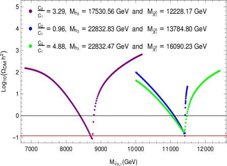
(a)

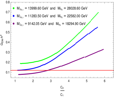
(b)

Figure 3: Relic density as a function of $M_{\tilde{\nu}_{R,1}}$ (left) and its dependence on the ratio of couplings $\frac{C_{2}}{C_{1}}$ (right) for different singlet Higgs masses. The red lines correspond to the limits on the dark matter abundance obtained by the Planck Collaboration, $\Omega_{\text{DM}}h^{2}=0.1188\pm 0.0010$.

In figure 3b we show the dependence of the relic density on the ratio of couplings $C_{2}/C_{1}$ for fixed mediator masses close to the resonance. This confirms our expectations from the previous Section: if $C_{2}$ is significantly larger than $C_{1}$, the relic density increases with $C_{2}$ because the increase of the mediator decay width over–compensates the increased coupling strength in the total annihilation cross section. If $C_{2}\ll C_{1}$ the width of the mediator is dominated by mediator decays into $\tilde{\nu}_{R,1}\tilde{\nu}^{*}_{R,1}$; hence increasing $C_{2}$ reduces the relic density because it increases the normalization of the annihilation cross section. Note that the relic density curve is fairly flat over some range of $C_{2}/C_{1}$. Moreover, the optimal choice of $C_{2}/C_{1}$ also depends somewhat on how far $M_{\tilde{\nu}_{R,1}}$ is below $M_{h_{3}}/2$. Altogether, for given $M_{h_{3}}$ there is an extended $1-$dimensional domain in the $(M_{\tilde{\nu}_{R,1}},C_{2}/C_{1})$ plane over which the relic density is quite close to its absolute minimum. This simplifies our task of minimization. Note also that we calculate the annihilation cross section only at tree–level; a change of the predicted relic density that is smaller than a couple of percent is therefore not really physically significant.

The parameters of the blue curve in Fig. 3b in fact are very close to those that maximize $M_{\tilde{\nu}_{R,1}}$ within the $U(1)_{\psi}$ model, under the assumption that $\tilde{\nu}_{R,1}$ was in thermal equilibrium in standard cosmology. $M^{\rm max}_{\tilde{\nu}_{R,1}}\simeq 11.5$ TeV corresponds to an upper bound on $M_{h_{3}}$ and $M_{Z^{\prime}}$ of about $23.0$ TeV. This is clearly beyond the reach of the LHC, and might even stretch the capabilities of proposed $100$ TeV $pp$ colliders.

Recall that all left–handed SM (anti)fermions have the same $U(1)_{\psi}$ charge. As a result, in the absence of $Z-Z^{\prime}$ mixing the $Z^{\prime}f\bar{f}$ couplings are purely axial vector couplings, for all SM fermions $f$. $Z^{\prime}$ exchange can therefore only contribute to spin–dependent WIMP–nucleon scattering in this model. Since our WIMP candidate doesn’t have any spin, $Z^{\prime}$ exchange does not contribute at all. Once $Z-Z^{\prime}$ mixing is included, $Z$ exchange contributes a term of order $M_{\tilde{\nu}_{R,1}}M_{N}\sin\alpha_{ZZ^{\prime}}/M_{Z}^{2}\propto M_{\tilde{\nu}_{R,1}}M_{N}/M_{Z^{\prime}}^{2}$ to the matrix element for $\tilde{\nu}_{R,1}N$ scattering, while the mixing–induced $Z^{\prime}$ exchange contribution is suppressed by another factor $M_{Z}^{2}/M_{Z^{\prime}}^{2}$; here $M_{N}$ is the mass of the nucleon. There is also a small contribution from the light SM–like Higgs boson $h_{1}$, which is very roughly of order $M_{N}^{2}/M_{h_{1}}^{2}$. As a result the scattering cross section on nucleons is very small, below $10^{-13}$ pb for the scenario that maximizes $M_{\tilde{\nu}_{R,1}}$. For the given large WIMP mass, this is not only several orders of magnitude below the current bound, but also well below the background from coherent neutrino scattering (“neutrino floor”).

4.3 The $U(1)_{\eta}$ Model

We now consider a value of $\theta_{E_{6}}$ with a larger $U(1)^{\prime}$ charge of the right–handed neutrino superfields. This increases the coupling $C_{1}$ for given $M_{Z^{\prime}}$, and thus the $\tilde{\nu}_{R,1}$ annihilation cross section for given masses, which in turn will lead to a weaker upper limit on $M_{\tilde{\nu}_{R,1}}$ from the requirement that the $\tilde{\nu}_{R,1}$ relic density not be too large.

In our analysis we therefore choose the SUSY breaking scale to be 50 TeV and we fix $\tan\beta=2.2$, and ${\bf m^{2}_{\tilde{Q}}}=1.28\times 10^{9}$ GeV${}^{2}\cdot{\bf 1},{\bf m^{2}_{\tilde{U}^{C}}}=1.45\times 10^{9}$ GeV${}^{2}\cdot{\bf 1}$, ${\bf m^{2}_{\tilde{D}^{C}}}=3.0\times 10^{9}$ GeV${}^{2}\cdot{\bf 1}$, ${\bf m^{2}_{\tilde{L}}}=3.0\times 10^{9}$ GeV${}^{2}\cdot{\bf 1}$, ${\bf m^{2}_{\tilde{E}^{C}}}=1.28\times 10^{9}$ GeV${}^{2}\cdot{\bf 1}$, $\left(m^{2}_{\tilde{N}^{C}}\right)_{22}=-4.0\times 10^{8}$ GeV², $\left(m^{2}_{\tilde{N}^{C}}\right)_{33}=-3.9\times 10^{8}$ GeV². To keep $M_{h_{1}}$ close to 125 GeV, the top trilinear coupling took values in the range ${T_{u,33}}=[-130,-114]$ TeV. In this case the $U(1)^{\prime}$ $D-$term contributions are positive for $\tilde{Q},\,\tilde{u}^{C}$ and $\tilde{\nu}_{R}$, but are negative for $\tilde{L}$ and $\tilde{d}^{C}$.

In this model the two Higgs doublets have different $U(1)^{\prime}$ charges; hence there is a sizable gauge contribution to the off–diagonal couplings of eq.(32). The Higgs doublet charges again have the opposite sign as the charge of $S$, leading to cancellations between the $\lambda^{2}$ and $g^{\prime 2}$ terms in the diagonal couplings (30) and (31). This cancellation is particularly strong for the coupling to two light states, so that for the interesting range of $\lambda$ the most important final states involve two heavy $SU(2)_{L}$ doublets, although final states with one light and one heavy boson are also significant. Partly because of this, and partly because the coefficients of the $g^{\prime 2}$ terms are smaller than in the $U(1)_{\psi}$ model, smaller values of the coupling $\lambda$ are required; the numerical results below have been obtained with $\lambda\in[0.260,0.352]$.

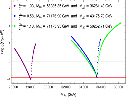
(a)

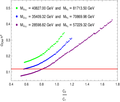
(b)

Figure 4: As in Fig. 3, but for the $U(1)_{\eta}$ model.

In Fig. 4 we again show the dependence of the relic density on the mass of the lightest RH sneutrino (left) and on the ratio of couplings $C_{2}/C_{1}$ (right). The qualitative behavior is similar to that in the $U(1)_{\psi}$ model depicted in Fig. 3, but clearly much larger values of $M_{\tilde{\nu}_{R,1}}$ are now possible, the absolute upper bound being near $35$ TeV (see the blue curves). The corresponding $Z^{\prime}$ mass of about $70$ TeV is definitely beyond the reach of a $pp$ collider operating at $\sqrt{s}=100$ TeV

Since $Q^{\prime}_{Q}=Q^{\prime}_{U^{C}}\neq Q^{\prime}_{D^{C}}$ in this model, there is no vector coupling of the $Z^{\prime}$ to up quarks, but such a coupling does exist for down quarks. Hence now the $Z^{\prime}$ exchange contribution to the matrix element for elastic scattering of $\tilde{\nu}_{R,1}$ on nucleons is comparable to that of $Z$ exchange once $Z-Z^{\prime}$ mixing has been included, and the $h_{1}$ exchange contribution has roughly the same size as in the $U(1)_{\psi}$ model. The total $\tilde{\nu}_{R,1}N$ scattering cross sections are again below $10^{-13}$ pb, for parameters near the upper bound on $M_{\tilde{\nu}_{R,1}}$. Since our WIMP candidate is now even heavier than in the $U(1)_{\psi}$ model, this is even more below the current constraints as well as below the neutrino floor.

4.4 The General UMSSM

In this subsection we investigate in more detail how the upper bound on $M_{\tilde{\nu}_{R,1}}$ depends on $\theta_{E_{6}}$. To this extent we have applied the procedure outlined in subsec. 4.1, and applied to two specific $U(1)^{\prime}$ models in subsecs. 4.2 and 4.3, to several additional $U(1)^{\prime}$ models, each with a different value of $\theta_{E_{6}}$.

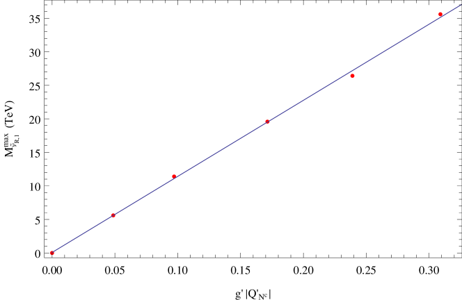
Figure 5: The upper limit on $M_{\tilde{\nu}_{R,1}}$ derived from the relic density as a function of $|Q^{\prime}_{N^{C}}|$. The straight line shows a linear fit to the six numerical results.

The results are shown in Fig. 5, where we plot the upper bound on the mass of the lightest RH sneutrino as a function of the absolute value of the product $g^{\prime}Q^{\prime}_{N^{C}}$. In order of increasing $|Q^{\prime}_{N^{C}}|$, the six red points correspond to the following choices of $\theta_{E_{6}}$:

$$\\ \biggl{\{}\arctan\sqrt{15},\frac{\left(\arctan\sqrt{15}+\frac{\pi}{2}\right)}{2},\frac{\pi}{2},\frac{\left(\arctan\sqrt{\frac{3}{5}}+\arctan\left[\frac{7}{\sqrt{15}}\right]\right)}{2},\arctan\sqrt{\frac{3}{5}},-\arctan\sqrt{\frac{5}{3}}\biggr{\}}\,.$$

Note that the first point has a vanishing $U(1)^{\prime}$ charge for the $N^{C}$ superfields, i.e. the resonance enhancement of the annihilation cross section does not work in this case. We checked that the cross section for elastic $\tilde{\nu}_{R,1}N$ scattering is well below the experimental bound for all other points.

Evidently the upper bound on $M_{\tilde{\nu}_{R,1}}$ scales essentially linearly with $Q^{\prime}_{N^{C}}$; recall that $g^{\prime}$ has been fixed to $\sqrt{5/3}g_{1}$ here. This linear dependence can be understood as follows. The $h_{3}\tilde{\nu}_{R,1}\tilde{\nu}_{R,1}^{*}$ coupling can be written as $g^{\prime}Q^{\prime}_{N^{C}}M_{Z^{\prime}}\simeq 2g^{\prime}Q^{\prime}_{N^{C}}M_{\tilde{\nu}_{R,1}}$. Moreover, we saw above that the maximal sneutrino mass is allowed if the effective final–state coupling $C_{2}$ is similar to $C_{1}$; it is therefore also proportional to $Q^{\prime}_{N^{C}}$. Therefore at the point where the bound is saturated, the $h_{3}$ decay width scales like $|C_{1}|^{2}M_{h_{3}}\propto g^{\prime 2}(Q^{\prime}_{N^{C}})^{2}M_{\tilde{\nu}_{R,1}}$, where we have again used that near the resonance all relevant masses are proportional to $M_{\tilde{\nu}_{R,1}}$. Note finally that for a narrow resonance – such as $h_{3}$, for the relevant parameter choices – the thermal average over the annihilation cross section scales like $1/(M_{h_{3}}\Gamma_{h_{3}})$ Griest:1990kh . Altogether we thus have

$$\langle\sigma v\rangle\propto\frac{|C_{1}C_{2}|^{2}}{M_{h_{3}}\Gamma_{h_{3}}M^{4}_{\tilde{\nu}_{R,1}}}\propto\frac{g^{\prime 2}(Q^{\prime}_{N^{C}})^{2}}{M^{2}_{\tilde{\nu}_{R,1}}}\,.$$ (38)

The linear relation between the upper bound on $M_{\tilde{\nu}_{R,1}}$ and $Q^{\prime}_{N^{C}}$ then follows from the fact that the thermally averaged annihilation cross section essentially fixes the relic density.

Note that here $Q^{\prime}_{N^{C}}$ always comes with a factor $g^{\prime}$; indeed, for a $U(1)$ gauge interaction only the product of gauge coupling and charge is well defined. The linear dependence of the bound on $M_{\tilde{\nu}_{R,1}}$ on $Q^{\prime}_{N^{C}}$ for fixed $g^{\prime}$ depicted in Fig. 5 can therefore also be interpreted as linear dependence of the bound on the product $g^{\prime}Q^{\prime}_{N^{C}}$. A fit to the points in Fig. 5 gives:

$$M^{\rm max}_{\tilde{\nu}_{R,1}}=(0.071+113.477g^{\prime}|Q^{\prime}_{N^{C}}|)\ {\rm TeV}\,.$$ (39)

This is the central result of our paper.

The highest absolute value of $|Q^{\prime}_{N^{c}}|$ in the UMSSM is about $0.82$, which is saturated for $\theta_{E_{6}}=-\arctan\left[\frac{1}{\sqrt{15}}\right]$. Using the linear fit of eq.(39) and $g^{\prime}=\sqrt{5/3}g_{1}=0.47$ leads to an absolute upper bound on $M_{\tilde{\nu}_{R,1}}$ in unifiable versions of the UMSSM of about $43.8$ TeV. This corresponds to an absolute upper bound on the $Z^{\prime}$ mass of about $87.6$ TeV.

Finally, we recall from eq.(19) that for $\theta_{E_{6}}$ between $-\arctan\sqrt{15}$ and $0$ one needs a negative squared soft breaking mass in order to have $M_{\tilde{\nu}_{R,1}}\simeq M_{Z^{\prime}}/2$. Since the $\hat{N}^{C}$ superfields appear in the superpotential (5) only multiplied with the tiny couplings ${\bf Y_{\nu}}$, this superpotential will not allow to generate negative squared soft breaking masses for sneutrinos via renormalization group running starting from positive values at some high scale. If we insist on positive squared soft breaking mass for all $\tilde{\nu}_{R}$ fields the upper bound on $|Q^{\prime}_{N^{C}}|$ is reduced to $\sqrt{5/8}\simeq 0.79$, in which case the bound on $M_{\tilde{\nu}_{R,1}}$ is reduced to about $42$ TeV. We note, however, that the $\hat{N}^{C}$ superfields can have sizable couplings to some of the exotic color triplets that reside in the ${\mathbf{2}7}-$dimensional representation Hewett:1988xc . Recalling that at least some of these exotic fermions are usually required for anomaly cancellation it should not be too difficult to construct a UV complete model that allows negative squared soft breaking terms for (some) $\tilde{\nu}_{R}$ at the SUSY mass scale.

4.5 Prospects for Detection

Clearly spectra near the upper bound presented in the previous subsection are not accessible to searches at the LHC, nor even to a proposed 100 TeV $pp$ collider.

As already noted for the $U(1)_{\eta}$ and $U(1)_{\psi}$ models the $\tilde{\nu}_{R,1}$ nucleon scattering cross section is very small. The very large $Z^{\prime}$ mass suppresses the $Z^{\prime}$ exchange contribution; as we saw in Sec. 2.3 it also suppresses $Z-Z^{\prime}$ mixing, so that the $Z$ exchange contribution also scales like $M_{Z^{\prime}}^{-2}$. The contribution due to the exchange of the singlet–like Higgs boson ($h_{3}$ in our analysis) is suppressed by the very large value of $M_{h_{3}}$ as well as the tiny $h_{3}q\bar{q}$ couplings, which solely result from mixing between singlet and doublet Higgs bosons. Finally, the contribution from the exchange of the doublet Higgs bosons, in particular of the 125 GeV state $h_{1}$, is suppressed by the small size of the $h_{1}\tilde{\nu}_{R,1}\tilde{\nu}_{R,1}^{*}$ coupling, which is of order $g^{\prime}v\ll M_{\tilde{\nu}_{R,1}}$, as well as the rather small $h_{1}q\bar{q}$ couplings, which are much smaller than gauge couplings. As a result, the $\tilde{\nu}_{R,1}$ nucleon scattering cross section, and hence the signal rate in direct WIMP detection experiments, is well below the neutrino–induced background; recall that this “neutrino floor” increases $\propto M_{\tilde{\nu}_{R,1}}$ since the WIMP flux, and hence the event rate for a given cross section, scales $\propto 1/M_{\tilde{\nu}_{R,1}}$.

The best chance to test these scenarios therefore comes from indirect detection. Naively one expects the cross section for annihilation from an $S-$wave initial state to be essentially independent of temperature, in which case the correct thermal relic density implies $\langle\sigma v\rangle\simeq 2.4\cdot 10^{-26}{\rm\text{ cm}}^{3}/{\rm\text{s}}\simeq 0.8{\rm\text{ pb}}\cdot\text{c}$ Steigman:2012nb ; Drees:2015exa . However, as pointed out in Ibe:2008ye ; Guo:2009aj this can change significantly in the resonance region; here the thermally averaged annihilation cross section can be significantly higher in today’s universe than at the time of WIMP decoupling.

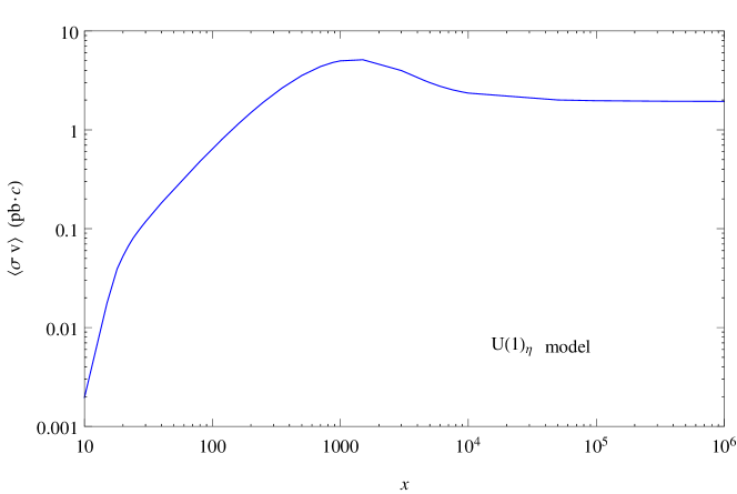
Figure 6: Thermally averaged cross section as a function of the scaled inverse temperature $x\equiv M_{\tilde{\nu}_{R,1}}/T$ for the parameters of the $U(1)_{\eta}$ model that saturate the upper bound on the sneutrino mass. Nominal decoupling occurs at $x=x_{F}=27.2$, whereas in today’s galaxies $x\sim 10^{6}$.

This is illustrated in Fig. 6 for the parameter choice that saturates the upper bound on $M_{\tilde{\nu}_{R,1}}$ in the $U(1)_{\eta}$ model. Here we show the thermally averaged $\tilde{\nu}_{R,1}\tilde{\nu}_{R,1}^{*}$ annihilation cross section times relative velocity as function of the scaled inverse temperature $x=M_{\tilde{\nu}_{R,1}}/T$. We see that for a quite extended range of temperatures around the decoupling temperature, $\langle\sigma v\rangle$ grows almost linearly with $x$. This is because $M_{\tilde{\nu}_{R,1}}$ is only slightly below the nominally resonant value $M_{h_{3}}/2$; by reducing the temperature the fraction of the velocity distribution that falls within approximately one $h_{3}$ decay width of the pole therefore at first increases.

Today’s relic density is essentially inversely proportional to the “annihilation integral”, defined as Griest:1990kh

$$J(x_{F})=\int_{x_{F}}^{\infty}\frac{\langle\sigma v\rangle}{x^{2}}dx\,.$$ (40)

An annihilation cross section that grows significantly for $x>x_{F}$ therefore has to be compensated by a smaller value of $\langle\sigma v\rangle(x_{F})$ in order to keep the relic density constant. As a result, in our scenarios the annihilation cross section at decoupling is actually significantly smaller than for typical $S-$wave annihilation.

Because for parameters that saturate the upper bound on $M_{\tilde{\nu}_{R,1}}$ the right-handed sneutrino mass is somewhat below $M_{h_{3}}/2$, for very large $x$, i.e. very small temperature, the thermally averaged annihilation cross section starts to decrease again. However, for the parameters of Fig. 6 it asymptotes to a value that is still about three times larger than the “canonical” thermal WIMP annihilating from an $S-$wave initial state. As shown in refs. Ibe:2008ye ; Guo:2009aj this enhancement factor strongly depends on $2M_{\tilde{\nu}_{R,1}}-M_{h_{3}}$; it can be even larger for slightly smaller sneutrino masses that are even closer to $M_{h_{3}}/2$.

The WIMP annihilation rate in today’s universe scales like the square of the WIMP number density. This means that the flux of annihilation products scales like $1/M^{2}_{\tilde{\nu}_{R,1}}$; for parameters (nearly) saturating our upper bound on the sneutrino mass it is thus too small to be detectable by space–based observatories like FermiLAT Ackermann:2015zua , simply because of their small size. Recall also that our sneutrinos annihilate into (longitudinal) gauge or Higgs bosons, and thus mostly into multi–hadron final states. This leads to a continuous photon spectrum which, for parameters near the upper bound on the sneutrino mass, extends well into the TeV region. Photons of this energy can be detected by Cherenkov telescopes on the ground, via their air showers. Note also that the astrophysical cosmic ray background drops even faster than $E^{-2}$ with increasing energy $E$ of the cosmic rays; the signal to background ratio therefore actually improves with increasing WIMP mass. Indeed, simulations show that at least for a favorable distribution of dark matter particles near the center of our galaxy, the continuum photon flux of multi–TeV WIMPs annihilating with the canonical thermal cross section should be detectable by the Cherenkov Telescope Array Carr:2015hta .

5 Summary and Conclusions

In this paper we analyzed the UMSSM, i.e. extensions of the minimal supersymmetrized Standard Model that contain an additional $U(1)^{\prime}$ gauge group as well as additional right–handed (RH) neutrino superfields which are singlets under the SM gauge group but carry $U(1)^{\prime}$ charge. We assume that $U(1)^{\prime}$ is a subgroup of $E_{6}$, which has been suggested as an (effective) GUT group, e.g. in the context of early superstring phenomenology. In this case the lightest RH sneutrino $\tilde{\nu}_{R,1}$ can be a good dark matter candidate.

We found that even within minimal cosmology, and fixing the $U(1)^{\prime}$ gauge strength to be equal to that of the hypercharge interaction of the (MS)SM (in GUT normalization), $\tilde{\nu}_{R,1}$ masses of tens of TeV are possible. For given $U(1)^{\prime}$ charges the bound on $M_{\tilde{\nu}_{R,1}}$ is saturated if $\tilde{\nu}_{R,1}$ can annihilate resonantly through the exchange of both the new $Z^{\prime}$ gauge boson and of the new Higgs boson $h_{3}$ associated with the spontaneous breaking of $U(1)^{\prime}$; note that $M_{Z^{\prime}}\simeq M_{h_{3}}$ automatically in this model. Scalar $h_{3}$ exchange is more important since $Z^{\prime}$ exchange can only occur from a $P-$wave initial state. The $h_{3}\tilde{\nu}_{R,1}\tilde{\nu}_{R,1}^{*}$ coupling is fixed by the $U(1)^{\prime}$ charge $Q^{\prime}_{N^{C}}$ of the right–handed neutrinos, but the $h_{3}$ couplings to the relevant final states can be tuned independently, allowing a further maximization of the annihilation cross section. In our analysis we used $SU(2)_{L}$ doublet Higgs bosons as well as longitudinal $W$ and $Z$ bosons as final states. While the light $SU(2)$ doublet Higgs states, including the longitudinal $W$ and $Z$ modes, are always accessible, we could have replaced the heavy Higgs doublet in the final state by some exotic fermions which in most cases are required to cancel anomalies. The only requirement is that the effective final state coupling of $h_{3}$ should be tunable to values close to its coupling to $\tilde{\nu}_{R,1}$. Since the $Z^{\prime}$ exchange contribution is basically fixed by $\theta_{E_{6}}$, and non–resonant contributions are negligible for $M_{\tilde{\nu}_{R,1}}\sim M_{Z^{\prime}}/2$, most of the many free parameters of this model, which describe the sfermion and gaugino sectors, are essentially irrelevant to us. The only requirement is that these superparticles are sufficiently heavy to avoid co–annihilation, which would increase the relic density in our case.

We found that the final upper bound on $M_{\tilde{\nu}_{R,1}}$ is essentially proportional to the product $g^{\prime}|Q^{\prime}_{N^{C}}|$, where $g^{\prime}$ is the $U(1)^{\prime}$ gauge coupling. Within the context of theories unifiable into $E_{6}$ this leads to an absolute upper bound on $M_{\tilde{\nu}_{R,1}}$ of about $43.8$ TeV. In other words, in this fairly well motivated set–up we can find a thermal WIMP candidate with mass less than a factor of three below the bound derived from unitarity Griest:1989wd . This is to be contrasted with an upper bound on the mass of a neutralino WIMP in the MSSM of about 8 TeV for unsuppressed co–annihilation with gluinos Ellis:2015vaa . In a rather more exotic model featuring a WIMP residing in the quintuplet representation of $SU(2)$ a WIMP mass of up to $9.6$ TeV is allowed Cirelli:2009uv .

Of course, this mechanism requires some amount of finetuning: the mass of the WIMP needs to be just below half the mass of the $s-$channel mediator. We find that typically the predicted WIMP relic density increases by a factor of $2$ when the WIMP mass is reduced by between $1$ and $3\%$ from its optimal value. In contrast, the recent proposal to allow thermal WIMP masses near $100$ TeV via non–perturbative co–annihilation requires finetuning to less than $1$ part in $10^{5}$ coan_new .

We also note that our very heavy WIMP candidates have very small scattering cross sections on nuclei, at least two orders of magnitude below the neutrino floor. This shows that both collider searches and direct WIMP searches are still quite far away from decisively probing this reasonably well motivated WIMP candidate. On the other hand, we argued that indirect signals for WIMP annihilation might be detectable by future Cherenkov telescopes. Our analysis thus motivates extending the search for a continuous spectrum of photons from WIMP annihilation into the multi–TeV range.

While the result (39) has been derived within UMSSM models that can emerge as the low–energy limit of $E_{6}$ Grand Unification, it should hold much more generally. To that end $g^{\prime}|Q^{\prime}_{N^{C}}|$ should be replaced by $g_{\chi\chi\phi}/m_{\phi}$, where $\chi$ is a complex scalar WIMP annihilating through the near resonant exchange of the real scalar $\phi$, $g_{\chi\chi\phi}$ being the (dimensionful) $\chi\chi^{*}\phi$ coupling. In order to saturate our bound the couplings of $\phi$ to the relevant final states should be tunable such that the effective final state coupling, which we called $C_{2}$ in Sec. 3, should be comparable to the initial–state coupling $g_{\chi\chi\phi}$. In this case the algorithm we used to find the upper limit on $M_{\tilde{\nu}_{R,1}}$, see subsec. 4.1, can directly be applied to finding the upper bound on $M_{\chi}$. We finally note that $M_{\chi}$ can be increased by another factor of $\sqrt{2}$ if $\chi$ is a real scalar.

- (1) U. Amaldi, W. de Boer and H. Fürstenau, Phys. Lett. B260 (1991) 447, doi:10.1016/0370-2693(91)91641-8
- (2) P. Langacker and M. x. Luo, Phys. Rev. D44 (1991) 817, doi:10.1103/PhysRevD.44.817.
- (3) J. R. Ellis, S. Kelley and D. V. Nanopoulos, Phys. Lett. B260 (1991) 131, doi:10.1016/0370-2693(91)90980-5
- (4) R. N. Mohapatra, hep-ph/9911272.
- (5) J. R. Ellis, J. S. Hagelin, D. V. Nanopoulos, K. A. Olive and M. Srednicki, Nucl. Phys. B238 (1984) 453, doi:10.1016/0550-3213(84)90461-9
- (6) G. Jungman, M. Kamionkowski and K. Griest, Phys. Rept. 267 (1996) 195, doi:10.1016/0370-1573(95)00058-5, hep-ph/9506380.
- (7) M. Tanabashi et al., Particle Data Group, Phys. Rev. D98 (2018) 030001.
- (8) E. Aprile et al., XENON Collaboration, arXiv:1805.12562 [astro-ph.CO].
- (9) G.B. Gelmini and P. Gondolo, Phys. Rev. D74, 023510 (2006), doi:10.1103/PhysRevD.74.023510, hep-ph/0602230.
- (10) E.W. Kolb and M.S. Turner, “The Early Universe”, Front.Phys. 69 (1990).
- (11) K. Griest and M. Kamionkowski, Phys. Rev. Lett. 64 (1990) 615, doi:10.1103/PhysRevLett.64.615.
- (12) P. A. R. Ade et al. [Planck Collaboration], Astron. Astrophys. 594 (2016) A13, doi:10.1051/0004-6361/201525830, arXiv:1502.01589 [astro-ph.CO].
- (13) J. Edsjo and P. Gondolo, Phys. Rev. D 56, 1879 (1997), doi:10.1103/PhysRevD.56.1879, hep-ph/9704361.
- (14) M. Cirelli, N. Fornengo and A. Strumia, Nucl. Phys. B753 (2006) 178, doi:10.1016/j.nuclphysb.2006.07.012, hep-ph/0512090.
- (15) M. Cirelli and A. Strumia, New J. Phys. 11 (2009) 105005, doi:10.1088/1367-2630/11/10/105005, arXiv:0903.3381 [hep-ph].
- (16) K. Griest and D. Seckel, Phys. Rev. D43 (1991) 3191, doi:10.1103/PhysRevD.43.3191.
- (17) C. Boehm, A. Djouadi and M. Drees, Phys. Rev. D62 (2000) 035012, doi:10.1103/PhysRevD.62.035012, hep-ph/9911496.
- (18) J. Harz and K. Petraki, JHEP 1807 (2018) 096, doi:10.1007/JHEP07(2018)096, arXiv:1805.01200 [hep-ph].
- (19) S. Biondini and M. Laine, JHEP 1804 (2018) 072, doi:10.1007/JHEP04(2018)072 arXiv:1801.05821 [hep-ph].
- (20) S. Profumo and C. E. Yaguna, Phys. Rev. D69 (2004) 115009, doi:10.1103/PhysRevD.69.115009, hep-ph/0402208.
- (21) J. Ellis, F. Luo and K. A. Olive, JHEP 1509 (2015) 127, doi:10.1007/JHEP09(2015)127 arXiv:1503.07142 [hep-ph].
- (22) H. Fukuda, F. Luo and S. Shirai, JHEP 1904 (2019) 107, doi:10.1007/JHEP04(2019)107, arXiv:1812.02066 [hep-ph].
- (23) M. Drees and M. M. Nojiri, Phys. Rev. D47 (1993) 376, doi:10.1103/PhysRevD.47.376, hep-ph/9207234.
- (24) J. E. Kim and H. P. Nilles, Phys. Lett. 138B (1984) 150, doi:10.1016/0370-2693(84)91890-2.
- (25) M. Cvetic, D. A. Demir, J. R. Espinosa, L. L. Everett and P. Langacker, Phys. Rev. D56 (1997) 2861, Erratum: Phys. Rev. D58 (1998) 119905, doi:10.1103/PhysRevD.56.2861, 10.1103/PhysRevD.58.119905, hep-ph/9703317.
- (26) U. Ellwanger, C. Hugonie and A. M. Teixeira, Phys. Rept. 496 (2010) 1, doi:10.1016/j.physrep.2010.07.001, arXiv:0910.1785 [hep-ph].
- (27) T. Han, P. Langacker and B. McElrath, Phys. Rev. D70 (2004) 115006, doi:10.1103/PhysRevD.70.115006, hep-ph/0405244.
- (28) J. L. Hewett and T. G. Rizzo, Phys. Rept. 183 (1989) 193, doi:10.1016/0370-1573(89)90071-9.
- (29) D. London and J. L. Rosner, Phys. Rev. D34 (1986) 1530, doi:10.1103/PhysRevD.34.1530.
- (30) H. S. Lee, K. T. Matchev and S. Nasri, Phys. Rev. D76 (2007) 041302, doi:10.1103/PhysRevD.76.041302, hep-ph/0702223.
- (31) D. G. Cerdeno, C. Munoz and O. Seto, Phys. Rev. D79 (2009) 023510, doi:10.1103/PhysRevD.79.023510, arXiv:0807.3029 [hep-ph].
- (32) R. Allahverdi, B. Dutta, K. Richardson-McDaniel and Y. Santoso, Phys. Lett. B677 (2009) 172, doi:10.1016/j.physletb.2009.05.034, arXiv:0902.3463 [hep-ph].
- (33) S. Khalil, H. Okada and T. Toma, JHEP 1107 (2011) 026, doi:10.1007/JHEP07(2011)026, arXiv:1102.4249 [hep-ph].
- (34) G. Bélanger, J. Da Silva and A. Pukhov, JCAP 1112 (2011) 014, doi:10.1088/1475-7516/2011/12/014, arXiv:1110.2414 [hep-ph].
- (35) G. Bélanger, J. Da Silva, U. Laa and A. Pukhov, JHEP 1509 (2015) 151, doi:10.1007/JHEP09(2015)151, arXiv:1505.06243 [hep-ph].
- (36) G. Bélanger, J. Da Silva and H. M. Tran, Phys. Rev. D95 (2017) 115017, doi:10.1103/PhysRevD.95.115017, arXiv:1703.03275 [hep-ph].
- (37) T. Falk, K. A. Olive and M. Srednicki, Phys. Lett. B339 (1994) 2 doi:10.1016/0370-2693(94)90639-4, hep-ph/9409270.
- (38) M. Drees, R. Godbole and P. Roy, “Theory and phenomenology of sparticles: An account of four-dimensional N=1 supersymmetry in high energy physics,” Hackensack, USA: World Scientific (2004).
- (39) W. Porod, Comput. Phys. Commun. 153 (2003) 275, doi:10.1016/S0010-4655(03)00222-4, hep-ph/0301101.
- (40) W. Porod and F. Staub, Comput. Phys. Commun. 183 (2012) 2458, doi:10.1016/j.cpc.2012.05.021, arXiv:1104.1573 [hep-ph].
- (41) F. Staub, arXiv:0806.0538 [hep-ph].
- (42) F. Staub, Comput. Phys. Commun. 185 (2014) 1773, doi:10.1016/j.cpc.2014.02.018 arXiv:1309.7223 [hep-ph].
- (43) F. Staub, Adv. High Energy Phys. 2015 (2015) 840780, doi:10.1155/2015/840780, arXiv:1503.04200 [hep-ph].
- (44) J. Kalinowski, S. F. King and J. P. Roberts, JHEP 0901 (2009) 066, doi:10.1088/1126-6708/2009/01/066, arXiv:0811.2204 [hep-ph].
- (45) S. F. King, S. Moretti and R. Nevzorov, Phys. Rev. D73 (2006) 035009, doi:10.1103/PhysRevD.73.035009, hep-ph/0510419.
- (46) Y. Okada, M. Yamaguchi and T. Yanagida, Prog. Theor. Phys. 85 (1991) 1, doi:10.1143/ptp/85.1.1
- (47) H. E. Haber and R. Hempfling, Phys. Rev. Lett. 66 (1991) 1815, doi:10.1103/PhysRevLett.66.1815
- (48) D. Suematsu, Phys. Lett. B416 (1998) 108, 10.1016/S0370-2693(97)01298-7, hep-ph/9705405.
- (49) D. Suematsu, Phys. Rev. D57 (1998) 1738, 10.1103/PhysRevD.57.1738, hep-ph/9708413.
- (50) J. M. Cornwall, D. N. Levin and G. Tiktopoulos, Phys. Rev. D10 (1974) 1145, doi:10.1103/PhysRevD.10.1145; C. E. Vayonakis, Lett. Nuovo Cim. 17 (1976) 383, doi:10.1007/BF02746538; B. W. Lee, C. Quigg and H. B. Thacker, Phys. Rev. D16 (1977) 1519, doi:10.1103/PhysRevD.16.1519; M. S. Chanowitz and M. K. Gaillard, Nucl. Phys. B261 (1985) 379, doi:10.1016/0550-3213(85)90580-2.
- (51) M. D. Goodsell, K. Nickel and F. Staub, doi:10.1140/epjc/s10052-014-3247-y, Eur. Phys. J. C75 (2015) 32, arXiv:1411.0675 [hep-ph].
- (52) M. Goodsell, K. Nickel and F. Staub, Eur. Phys. J. C75 (2015) 290, doi:10.1140/epjc/s10052-015-3494-6, arXiv:1503.03098 [hep-ph].
- (53) J. Braathen, M. D. Goodsell and F. Staub, Eur. Phys. J. C77 (2017) 757, doi:10.1140/epjc/s10052-017-5303-x, arXiv:1706.05372 [hep-ph].
- (54) G. Bélanger, F. Boudjema, A. Pukhov and A. Semenov, Comput. Phys. Commun. 192 (2015) 322, doi: 10.1016/j.cpc.2015.03.003, arXiv:1407.6129 [hep-ph].
- (55) G. Bélanger, N. D. Christensen, A. Pukhov and A. Semenov, Comput. Phys. Commun. 182 (2011) 763, doi:10.1016/j.cpc.2010.10.025, arXiv:1008.0181 [hep-ph].
- (56) A. Pukhov, hep-ph/0412191.
- (57) A. Belyaev, N. D. Christensen and A. Pukhov, Comput. Phys. Commun. 184 (2013) 1729, doi:10.1016/j.cpc.2013.01.014, arXiv:1207.6082 [hep-ph].
- (58) F. Staub, T. Ohl, W. Porod and C. Speckner, Comput. Phys. Commun. 183 (2012) 2165, doi:10.1016/j.cpc.2012.04.013, arXiv:1109.5147 [hep-ph].
- (59) P. Langacker and J. Wang, Phys. Rev. D58 (1998) 115010, doi:10.1103/PhysRevD.58.115010, hep-ph/9804428.
- (60) M. Carena, S. Heinemeyer, O. Stal, C. E. M. Wagner and G. Weiglein, Eur. Phys. J. C73 (2013) 2552, doi:10.1140/epjc/s10052-013-2552-1.
- (61) G. Steigman, B. Dasgupta and J. F. Beacom, Phys. Rev. D 86 (2012) 023506 doi:10.1103/PhysRevD.86.023506.
- (62) M. Drees, F. Hajkarim and E. R. Schmitz, JCAP 1506 (2015) no.06, 025 doi:10.1088/1475-7516/2015/06/025.
- (63) M. Ibe, H. Murayama and T. T. Yanagida, Phys. Rev. D 79 (2009) 095009, doi:10.1103/PhysRevD.79.095009.
- (64) W. L. Guo and Y. L. Wu, Phys. Rev. D 79 (2009) 055012, doi:10.1103/PhysRevD.79.055012.
- (65) M. Ackermann et al. [Fermi-LAT Collaboration], Phys. Rev. Lett. 115 (2015) no.23 231301, doi:10.1103/PhysRevLett.115.231301.
- (66) J. Carr et al. [CTA Collaboration], PoS ICRC 2015 (2016) 1203, doi:10.22323/1.236.1203, arXiv:1508.06128 [astro-ph.HE].