Probing Baryogenesis through the Higgs Self-Coupling

Abstract

The link between a modified Higgs self-coupling and the strong first-order phase transition necessary for baryogenesis is well explored for polynomial extensions of the Higgs potential. We broaden this argument beyond leading polynomial expansions of the Higgs potential to higher polynomial terms and to non-polynomial Higgs potentials. For our quantitative analysis we resort to the functional renormalization group, which allows us to evolve the full Higgs potential to higher scales and finite temperature. In all cases we find that a strong first-order phase transition manifests itself in an enhancement of the Higgs self-coupling by at least 50%, implying that such modified Higgs potentials should be accessible at the LHC.

I Introduction

The existence of a scalar Higgs potential is the most fundamental insight from the LHC to date. It is based on the observation of a likely fundamental Higgs scalar in combination with measurements of the massive electroweak bosons, fixing the infrared theory and its model parameters after electroweak symmetry breaking to high precision. The one remaining parameter is the Higgs self-coupling and its relation to the Higgs mass, defining a standard benchmark measurement for current and future colliders. This in itself very interesting measurement may also be related to more fundamental physics questions. A prime candidate for such a question is electroweak baryogenesis, specifically the nature of the electroweak phase transition.

For the single Higgs boson of the renormalizable Standard Model we can test the electroweak phase transition through the Higgs mass. Here, electroweak baryogenesis ew_phase ; review_ew requires a Higgs mass well below the observed value of 125 GeV misha_higgs ; ew_higgs ; Shaposhnikov:1991cu . Only then will the electroweak phase transition be strongly first order. If we consider the Standard Model an effective field theory (EFT), a sizable dimension-6 contribution to the Higgs potential, $(\phi^{\dagger}\phi)^{3}/\Lambda^{2}$, is known to circumvent this bound eft1 ; eft2 ; Noble ; christophe_geraldine . In principle, this scenario can be tested through a measurement of the Higgs self-coupling at colliders uli1 ; eft2 ; Noble ; christophe_geraldine . The problem with this link is that the new-physics scale required by a first-order phase transition is typically not large, $\Lambda\gtrsim v=246$ GeV. If LHC data should indeed point to a dimension-6 Lagrangian with a low new-physics scale, we will see this in many other channels long before we will actually measure the Higgs self-coupling legacy . As a matter of fact, a global analysis of the effective Higgs Lagrangian including $(\phi^{\dagger}\phi)^{3}/\Lambda^{2}$ might never probe the required values of the Higgs self-coupling once we take into account all operators and all uncertainties, so it hardly serves as a motivation to measure a SM-like Higgs self-coupling.

In this paper we take a slightly different approach. First, we assume that the new physics responsible for the strongly first-order electroweak phase transition only appears in the Higgs sector. In the EFT framework we would consider, for example, the operator $(\phi^{\dagger}\phi)^{3}/\Lambda^{2}$ christophe_geraldine ; eft2 ; Noble . While this approach systematically includes higher-dimensional operators in a power-counting expansion, it is not at all guaranteed that such an expansion is appropriate for the underlying new physics. Furthermore, a description of first-order phase transitions requires one to extract global information about the effective potential. Again, a simple polynomial expansion around a vanishing Higgs field might not be sufficient to resolve the fluctuation-driven competition between different minima of the effective potential that induce a first-order phase transition.

A simple global approximation to the effective potential is provided by mean-field theory, which works remarkably well for Standard Model parameters mean-field ; Gies:2013fua ; Borchardt:2016xju ; Sondenheimer:2017jin because of the dominance of the top quark. Depending, however, on the strength of the bosonic and order-parameter fluctuations in the new physics model, mean-field approaches may become unreliable. We demonstrate this explicitly using a simple example case in this paper. This situation calls for non-perturbative methods. Recently, lattice simulations have been used to study the possibility of first-order phase transition in the presence of the operator $(\phi^{\dagger}\phi)^{3}/\Lambda^{2}$, both in a Higgs-Yukawa model Akerlund:2015fya and in a gauged-Higgs system Akerlund:2015gfy .

Here we use the functional renormalization group (FRG) christof_eq as a non-perturbative tool, for reviews see, e.g. , rg_reviews . It is able to provide global information about the Higgs potential, bridge a wide range of scales, include fluctuations of bosonic and fermionic matter fields as well as gauge bosons and deal with extended classes of Higgs potentials. The two questions which will guide us are:

1. Do extended Higgs potentials help with electroweak baryogenesis?

2. Can they be systematically tested by measuring the Higgs self-coupling?

We study the influence of operators or functions of operators in the Higgs sector on the electroweak phase transition using several representative examples. We determine the consequences for the Higgs self-coupling for suitable extended Higgs potentials supporting electroweak baryogenesis and being compatible with the standard-model mass spectrum.

The global properties of the Higgs potential are also intimately related to the questions of vacuum stability and Higgs mass bounds Krive:1976sg ; Lindner:1985uk ; Buttazzo:2013uya . In fact, higher-dimensional operators can also increase the stability regime of the vacuum Branchina:2005tu ; Gies:2013fua ; eichhorn_scherer ; our_paper ; Akerlund:2015fya ; stable_frg ; Jakovac:2015kka . The example Higgs potentials studied in this paper suggest new-physics scales well below a possible instability scale of $10^{10\cdots 12}$ GeV of the Standard Model. While vacuum instability is therefore not an issue for our study, extended potentials generally do have the potential to both support electroweak baryogenesis and stabilize the Higgs vacuum. A measurement of the Higgs self-coupling can therefore be indicative for both aspects.

I.1 Electroweak phase transition

The asymmetry between the matter and anti-matter contents in the Universe is one of the great mysteries in cosmology and particle physics. Experimentally, the effective absence of anti-matter in the Universe has been proven in many different ways antimatter_meas . A quantitative measurement is given by the baryon-to-photon ratio $n_{B}/n_{\gamma}\approx 6\cdot 10^{-10}$, which is many orders of magnitude larger than what we would expect from the thermal history in the presence of anti-matter. It can be explained by a small initial asymmetry in the number of baryons and anti-baryons which leads to a finite density of baryons after essentially all anti-baryons have annihilated away.

Theoretically, the mechanisms behind the baryon asymmetry are well understood. Most notably, it can be shown that the presence of an asymmetry is equivalent to the three Sakharov conditions for our fundamental theory ew_phase : baryon number violation, C as well as CP violation, and departure from thermal equilibrium. The first two conditions can be probed by precision measurements of the Lagrangian of the Standard Model and its extensions. The third condition can in principle be achieved at the time of the electroweak phase transition, where it then requires a strong first-order phase transition. The nature of the electroweak phase transition can be read off from the scalar potential in or beyond the Standard Model.

The strength of the phase transition which occurs at the critical temperature $T_{c}$ is measured by the ratio $\phi_{c}/T_{c}$, where $\phi_{c}=\langle\phi\rangle_{T_{c}}$ is the expectation value of the Higgs at the critical temperature. The critical temperature describes the transition where for small temperatures $T<T_{c}$ the potential exhibits a single, non-trivial minimum for some value of the scalar field $\phi$. The field value at the minimum is temperature dependent, approaching $v=246$ GeV for $T\rightarrow 0$. With increasing temperature, a second minimum at zero field value and with an unbroken electroweak symmetry appears in a first-order scenario. At the critical temperature $T_{c}$, the two minima of the potential, i.e. the one at finite field value and the one at vanishing field value are degenerate, and the system undergoes a phase transition from the symmetry-broken regime with a finite Higgs expectation value to the symmetric regime.

The field value at the minimum constitutes an order parameter. For $\phi_{c}\neq 0$ the transition is of first order, i.e. the vacuum does not evolve continuously through the phase transition. For electroweak baryogenesis, the transition has to be a strong first-order one,

$$\frac{\phi_{c}}{T_{c}}\gtrsim 1\,,$$ (1)

otherwise the baryon asymmetry is washed out Shaposhnikov:1991cu .

I.2 Higgs self-coupling measurement

Figure 1: Feynman diagrams contributing to Higgs pair production at the LHC. Figure from Ref. uli1 .

At energy scales relevant for the LHC, the self-interaction of the Higgs boson is described by the infrared (IR) Higgs potential in the broken phase. In the renormalizable Standard Model, and ignoring Goldstone modes, it reads at tree level

$$V=\frac{\mu^{2}}{2}\,(v+H)^{2}+\frac{\lambda_{4}}{4}\,(v+H)^{4}\;,$$ (2)

where $H$ is the physical Higgs field. The two parameters describing the SM-Higgs potential in the IR, $\mu$ and $\lambda_{4}$, can be traded for the vacuum expectations value $v$ and the Higgs mass $m_{H}$ lecture

$$v=\sqrt{\frac{\mu^{2}}{2\lambda_{4}}}=246~{}\text{GeV}\,,\qquad\qquad\qquad m_{H}=\sqrt{2\lambda_{4}}\,v=125~{}\text{GeV}\;.$$ (3)

The interaction between three and four physical Higgs bosons in the Standard Model is then given by

$$\lambda_{H^{3},0}=\frac{3m_{H}^{2}}{v}\,,\qquad\qquad\qquad\lambda_{H^{4},0}=\frac{3m_{H}^{2}}{v^{2}}\;.$$ (4)

In the limit of heavy top quarks, $2m_{t}>m_{H}$, an effective Higgs–gluon Lagrangian low_energy

$$\mathcal{L}_{ggH}=\frac{\alpha_{s}}{12\pi}\;G^{\mu\nu}G_{\mu\nu}\;\log\left(1+\frac{H}{v}\right)=\frac{\alpha_{s}}{12\pi}\;G^{\mu\nu}G_{\mu\nu}\;\frac{1}{v}\;\left(H-\frac{H^{2}}{2v}+\ldots\right)\,,$$ (5)

with the gluon field strength tensor $G_{\mu\nu}$ and the strong coupling $\alpha_{s}$, can be used to describe many relevant LHC observables.

When we include new physics contributions in the Higgs potential, the relations in Eq.(3) change. It is instructive to follow the simple example of the modified Higgs potential lecture

$$V=\frac{\mu^{2}}{2}\,(v+H)^{2}+\frac{\lambda_{4}}{4}\,(v+H)^{4}+\frac{\lambda_{6}}{\Lambda^{2}}\,(v+H)^{6}\;.$$ (6)

The modified relations between the observables become

$$m_{H} =\sqrt{2\lambda_{4}}\,v\left(1+12\frac{\lambda_{6}v^{2}}{\lambda_{4}\Lambda^{2}}\right)\,,$$

$$\lambda_{H^{3}} =\frac{3m_{H}^{2}}{v}\left(1+\frac{16\lambda_{6}v^{4}}{m_{H}^{2}\Lambda^{2}}\right)\equiv\lambda_{H^{3},0}\left(1+\frac{16\lambda_{6}v^{4}}{m_{H}^{2}\Lambda^{2}}\right)\,,$$

$$\lambda_{H^{4}} =\frac{3m_{H}^{2}}{v^{2}}\left(1+\frac{96\lambda_{6}v^{4}}{m_{H}^{2}\Lambda^{2}}\right)\equiv\lambda_{H^{4},0}\left(1+\frac{96\lambda_{6}v^{4}}{m_{H}^{2}\Lambda^{2}}\right)\;.$$ (7)

Because $m_{H}$ and $v$ have to keep their measured values, we need to adjust $\lambda_{4}$ to compensate for the effect of $\lambda_{6}$ on the Higgs mass. This shift has to be accounted for in the expressions for the Higgs self-couplings as a function of $m_{H}$ and $v$. The reference couplings $\lambda_{H^{n},0}$ keep their Standard Model values in terms of the unchanged parameters $m_{H}$ and $v$, but the physical Higgs couplings $\lambda_{H^{n}}$ change.

The standard channel to measure $\lambda_{H^{3}}$ at the LHC is Higgs pair production in gluon fusion, as illustrated in Fig. 1, orig ; spirix ; uli1 ; uli2 ; uli3 ; review_hh . Its production rate is known including NLO nlo and NNLO nnlo . One of the problems with such a measurement is that the link between the total di-Higgs production rate and the Higgs self-coupling requires us to know the top Yukawa coupling. An appropriate framework is the global Higgs analysis legacy ; hh_d6 , which is expected to give at best a 10% measurement of the top Yukawa coupling. A model-independent precision measurement of the top Yukawa coupling at the percent level will only be possible at a 100 TeV collider nimatron_yt .

The experimental situation improves once we include kinematic information in the di-Higgs production process. Two kinematic regimes are well known to carry information on the Higgs self-coupling, both exploiting the (largely) destructive interference between the two graphs shown in Fig. 1. While the continuum contribution dominates over most of the phase space, the two diagrams become comparable close to threshold spirix ; uli1 . The low-energy theory of Eq.(5) gives us for the combined di-Higgs amplitude

$$\mathcal{A}\propto\frac{\alpha_{s}}{12\pi v}\;\left(\frac{\lambda_{H^{3}}}{s-m_{H}^{2}}-\frac{1}{v}\right)\stackrel{{\scriptstyle\lambda_{H^{3}}=\lambda_{H^{3},0}}}{{\longrightarrow}}\frac{\alpha_{s}}{12\pi v^{2}}\;\left(\frac{3m_{H}^{2}}{3m_{H}^{2}}-1\right)=0\qquad\text{for}\quad m_{HH}\to 2m_{H}\;,$$ (8)

where $m_{HH}$ is the invariant di-Higgs mass. An exact cancellation occurs in the Standard Model. Whereas the heavy-top approximation is known for giving completely wrong kinematic distributions for Higgs pair production uli1 , it does correctly predict this threshold behavior. Note, that the momenta of the outgoing particles in such processes are typically small compared to the Higgs mass and the low-energy regime of the theory is probed. In the analysis in Sec. III, we thus read off the Higgs self-couplings from the low-energy effective potential.

The second relevant kinematic regime is boosted Higgs pair production boosted , because of top threshold contributions to the triangle diagram around $m_{HH}=2m_{t}$. In terms of the transverse momentum this happens around $p_{T,H}\approx 100$ GeV, where the combined amplitude develops a minimum for large Higgs self-couplings.

At the LHC, we define di-Higgs signatures simply based on Higgs decay combinations. The most promising channel is the $b\bar{b}\gamma\gamma$ final state uli3 ; madmax ; vernon ; atlas , where we can easily reconstruct one of the two Higgs bosons and measure the continuum background in the side bands. We can also use the $b\bar{b}\tau\tau$ final state uli2 ; boosted , assuming very efficient tau-tagging. The combination $b\bar{b}WW$ bbww requires an efficient suppression of the $t\bar{t}$ background, while the $4b$ uli2 ; bbbb and $4W$ uli1 ; wwww signatures are unlikely to work for SM-like Higgs bosons. Finally, the $b\bar{b}\mu\mu$ is in many ways similar for the $b\bar{b}\gamma\gamma$ channel uli3 , but with a much lower rate in the Standard Model.

To get an idea of what to expect, we quote the optimal reach of the high-luminosity LHC run with $3~{}\text{ab}^{-1}$, based on the Neyman-Pearson theorem applied to the $b\bar{b}\gamma\gamma$ channel for self-couplings relatively close to the Standard Model madmax ,

$$\frac{\lambda_{H^{3}}}{\lambda_{H^{3},0}} =\phantom{-}0.4~{}...~{}1.7\qquad\text{at 68\% CL,}$$ (9)

so any value for $\lambda_{H^{3}}/\lambda_{H^{3},0}$ outside the range given above will not be compatible with the vanishing di-Higgs amplitude in Eq.(8). This reach will be improved when we combine several Higgs decay channels, but will also suffer from systematic uncertainties. In addition, it assumes a perfect knowledge of the top Yukawa coupling. This implies that models which predict a change in the Higgs self-coupling by less than 50% will not be testable at the LHC.

II Modified Higgs potentials

Similar to the EFT approach we assume that beyond an ultraviolet (UV) scale or cutoff scale $\Lambda$ new physics exists and modifies the form of the Higgs potential. As the additional degrees of freedom are heavy, their effects below $\Lambda$ can be parametrized by additional terms in the Higgs potential, without modifying the propagating degrees of freedom. The details of the new physics are encoded in the initial condition for the RG flow of the Standard Model at $k=\Lambda$. Exploring different higher-order terms thus provides access to large classes of high-scale physics scenarios, for which we do not have to investigate the detailed matching of the additional terms in the Higgs potential and the underlying high-scale degrees of freedom at $k=\Lambda$.

Our system features three relevant energy scales. First, the RG scale $k$ ranges between $k=0$, where all quantum fluctuations are taken into account, and $k=\Lambda$, where we initialize the flow. Second, the temperature $T$ defines the external physics scale with which we probe our system. Third, the field value $\phi$ defines an additional, internal energy scale of our system. As is usual in EFT analyses, it is important to clearly disentangle these three scales, even though $\phi$ and $T$ can in principle act similarly to the RG scale $k$ in that they suppress IR quantum fluctuations our_paper . We employ a method that can straightforwardly account for the RG flow in the presence of these different scales, namely the functional renormalization group. In this setting, quantum fluctuations in the presence of further internal and external scales are taken into account by a functional differential equation that is structurally one-loop, without being restricted to a weak-coupling regime. This provides access to classes of non-perturbative microscopic models with a manageable computational effort. Most importantly, the functional RG approach enables us to keep track of the separate dependence of the potential on the RG scale $k$, the temperature and the field value even in cases with non-perturbative UV potentials, where, e.g. a mean-field approach breaks down.

For our study, we concentrate on that part of the Standard Model which is relevant for the RG flow of the Higgs potential using the framework developed in our_paper . Here, we follow that framework by implementing the effects of weak gauge bosons through a fiducial coupling, and upgrade our treatment by including a thermal mass generated by the corresponding fluctuations as their leading contribution instead of implementing a fully-fledged dynamical treatment of that sector, see App. A for details. Similarly, would-be Goldstone modes do not need to be considered explicitly, such that it suffices to concentrate on a real scalar field $\phi$, which after electroweak symmetry breaking can be described in terms of the physical Higgs field $H$ as $\phi=H+v$. At the UV scale $k=\Lambda$, the Higgs-potential is parametrized as

$$V_{k=\Lambda}=\frac{\mu^{2}}{2}\,\phi^{2}+\frac{\lambda_{4}}{4}\,\phi^{4}+\Delta V\,,$$ (10)

where $\Delta V$ contains the contribution of some higher dimensional operator. In principle, higher-order modifications of the Yukawa sector could also be included, cf. Pawlowski:2014zaa ; deVries:2017ncy ; Gies:2017zwf . We investigate three classes of modifications to the SM-Higgs potential:

1. additional $\phi^{6}$ or $\phi^{8}$ terms, which cover the leading-order terms in an effective-field theory approach and have been extensively studied in the literature eft1 ; christophe_geraldine ; eft2 ; Noble ;

2. a logarithmic dependence on the Higgs-field, inspired by Coleman-Weinberg potentials. It does not allow for a Taylor expansion around $\phi=0$. Logarithmic modifications are naturally generated by functional determinants, i.e. by integrating out heavy scalars or fermions.

3. a simple example of non-perturbative contributions of the form $\exp(-1/\phi^{2})$, i.e. an exponential dependence on the inverse field, consequently not admitting a Taylor expansion in the field around $\phi=0$. This is inspired by semiclassical contributions to the path integral with $\phi$ reminiscent to a moduli parameter of an underlying model.

We denote these modifications of the potential by

$$\Delta V_{6} =\lambda_{6}\,\frac{\phi^{6}}{\Lambda^{2}}\,,\qquad\qquad\qquad \Delta V_{8} =\lambda_{6}\,\frac{\phi^{6}}{\Lambda^{2}}+\lambda_{8}\,\frac{\phi^{8}}{\Lambda^{4}}\,,$$

$$\Delta V_{\ln,2} =-\lambda_{\ln,2}\,\frac{\phi^{2}\Lambda^{2}}{100}\;\ln\frac{\phi^{2}}{2\Lambda^{2}}\,,\qquad\qquad\qquad \Delta V_{\ln,4} =\lambda_{\ln,4}\,\frac{\phi^{4}}{10}\;\ln\frac{\phi^{2}}{2\Lambda^{2}}\,,$$

$$\Delta V_{\exp,4} =\lambda_{\exp,4}\phi^{4}\exp\left(-\frac{2\Lambda^{2}}{\phi^{2}}\right)\,,\qquad\qquad\qquad \Delta V_{\exp,6} =\lambda_{\exp,6}\frac{\phi^{6}}{\Lambda^{2}}\exp\left(-\frac{2\Lambda^{2}}{\phi^{2}}\right)\,.$$ (11)

In all these potentials $\Lambda$ describes a new physics scale, which absorbs the mass dimension of the Higgs field. The case of $\phi^{6}/\Lambda^{2}$ has been explored in the literature eft2 ; Noble ; christophe_geraldine and serves as a test of our method, as discussed in the Appendix. Neither the logarithmic nor the exponential potentials can be expanded around $\phi=0$, so they cannot be treated in an EFT framework. Similar bare potentials have been suggested in Sondenheimer:2017jin in the context of Higgs mass bounds and vacuum stability. Instead, all potentials that can be expanded around $\phi=0$ can be approximated by the power-ordered, first kind of potentials. As expected by canonical power counting, terms of higher order in $\phi$ can only play a role for very low values of $\Lambda/v$, unless their prefactors are non-perturbatively large. From a more general viewpoint, the set of power law, logarithmic and exponential potential functions does not only reflect the physics structures arising from local vertex expansions, one-loop determinants or semiclassical approximations. It also includes the set of functions to be expected on mathematical grounds if the effective potential permits a potentially resurgent transseries expansion Dunne:2012ae .

To investigate the different classes of modifications, a variety of tools appears to be at our disposal, a priori ranging from mean-field techniques to non-perturbative lattice tools and functional methods. It turns out that the former are only applicable to a restricted class of potentials, not allowing us to adequately explore the full range of possible UV potentials corresponding to diverse underlying microscopic models. This is displayed in Fig. 2 where the $\phi^{6}$- modification of the Higgs potentials shows the expected physical behavior as the strength of the first-order phase transition is decreasing with an increasing cutoff. The logarithmic modifications on the other hand show a rather unphysical behavior as the strength of the first-order phase transition remains constant or even increases with the UV scale. This indicates that scalar order-parameter fluctuations are important, which are ignored in simple mean-field theory. Therefore we make use of powerful functional techniques, which treat bosonic and fermionic fluctuations on the same footing.

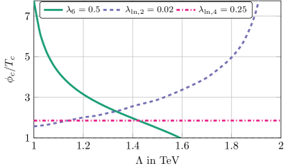
Figure 2: Mean-field results for $\phi_{c}/T_{c}$ as a function of the cutoff for different modifications of the Higgs potential. Second-order and weak first-order phase transitions are excluded from the plot. The results of the $\phi^{6}$ modification are reasonable, while the results for the $\phi^{2}\ln\phi^{2}$ and the $\phi^{4}\ln\phi^{2}$ modifications are clearly unphysical, see explanation in the text. More elaborate methods than mean-field are needed.

When allowing for modifications of the Higgs potential, we need to ensure that at $T=0$ the IR-values for $\mu$, $\lambda_{4}$, and the top-Yukawa-coupling $y_{t}$ are such that the measured observables do not change. We adjust the corresponding masses to

$$v=246\,\text{GeV}\,,\qquad\qquad\qquad m_{H}=125\,\text{GeV}\,,\qquad\qquad\qquad m_{t}=173\,\text{GeV}\,.$$ (12)

Within our numerical analysis, we require $v$ and $m_{t}$ to be reproduced to an accuracy of $\pm$0.5 GeV. The Higgs mass is adjusted within a somewhat larger numerical band of $\pm 1.5$ GeV. Since it is related to the second derivative (curvature) of the potential at the minimum, a higher precision is numerically more expensive, see App. B for details. Moreover, it is expected that the curvature mass used here shows small deviations from the Higgs pole mass $m_{H}$, see Helmboldt:2014iya , and the above band also contains an estimate of this systematic error. In the symmetry broken regime, the potential given in Eq.(10) can be expanded in powers of $(\phi^{2}-v^{2})$. In the decoupling region in the deep IR, we use the parametrization

$$V_{k\ll v} =\frac{\lambda_{4,\,\rm IR}}{4}(\phi^{2}-v^{2})^{2}+\frac{\lambda_{6,\,\rm IR}}{8v^{2}}(\phi^{2}-v^{2})^{3}+\frac{\lambda_{8,\,\rm IR}}{16v^{4}}(\phi^{2}-v^{2})^{4}+\cdots$$

$$=\lambda_{4,\,\rm IR}v^{2}H^{2}+\left(\lambda_{4,\,\rm IR}+\lambda_{6,\,\rm IR}\right)vH^{3}+\frac{1}{4}\left(\lambda_{4,\,\rm IR}+6\lambda_{6,\,\rm IR}+4\lambda_{8,\,\rm IR}\right)H^{4}+\cdots\,.$$ (13)

Note that this is the full effective potential in the IR, differing from the tree-level potential in Eq.(6). In particular, higher-order terms, encoded in $\lambda_{6,\,\rm IR}$ are generated by quantum fluctuations even if the tree-level potential is quartic. At tree level, the Higgs potential is described by two parameters, i.e. $\lambda_{6,\,\rm IR}=\lambda_{8,\,\rm IR}=\ldots=0$. If we allow higher-order terms, all measurable parameters are affected, in close analogy to Eq.(7). As described in Sec. I.2 the vacuum expectation value $v$ and the Higgs mass $m_{H}^{2}/(2v^{2})\equiv\lambda_{4}$ are known very precisely from collider measurements and thus we have to keep them fixed. The physical Higgs self-couplings change from the values given in Eq.(4) to the more general form

$$\lambda_{H^{3}}=\frac{\delta^{3}}{\delta H^{3}}V_{k=0}=6v(\lambda_{4,\,\rm IR}+\lambda_{6,\,\rm IR})\,,\qquad\lambda_{H^{4}}=\frac{\delta^{4}}{\delta H^{4}}V_{k=0}=6(\lambda_{4,\,\rm IR}+6\lambda_{6,\,\rm IR}+4\lambda_{8,\,\rm IR})\;.$$ (14)

The first terms are precisely the couplings $\lambda_{H^{3},0}=6v\lambda_{4,\,\rm IR}$ and $\lambda_{H^{4},0}=6\lambda_{4,\,\rm IR}$ familiar from the tree-level structure. With the present setup we can compute the Higgs self-couplings in the pure Standard Model including higher-order terms generated by quantum fluctuations by initializing the flow at some high cutoff scale without any modifications of the Higgs potential. As long as the cutoff is not too close to the electroweak scale the results will be largely independent of the cutoff choice. For our level of numerical precision, a cutoff $\Lambda=2$ TeV is sufficient. The Higgs self-couplings are given by

$$\frac{\lambda_{H^{3}}}{\lambda_{H^{3},0}}\approx 0.92\,,\qquad\qquad\qquad\frac{\lambda_{H^{4}}}{\lambda_{H^{4},0}}\approx 0.68\;.$$ (15)

These values are equivalent to computations of the Higgs potential with Coleman-Weinberg corrections. We then go beyond the pure Standard Model by adjusting a combination of the coefficients $\lambda_{j}$ and the new physics scale $\Lambda$ in Eq.(11). These can now be used to adjust $\phi_{c}/T_{c}$ such that we obtain a strong first-order phase transition.

III Phase transition

For the modified Higgs potentials defined in Eq.(11) we need to explore which values of the UV scale $\Lambda$ and the coefficients $\lambda_{j}$ lead to a sufficiently strong first-order transition. Simultaneously, we monitor whether this leads to a measurable modification of the Higgs self-couplings in the IR.

III.1 First-order phase transition

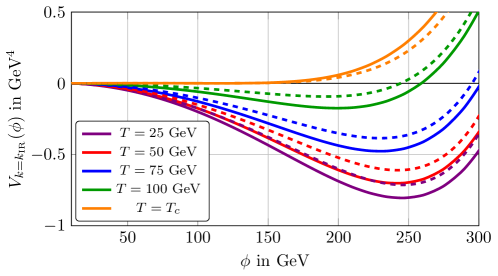
Figure 3: Temperature evolution of the potentials of the type $\phi^{4}\ln\phi^{2}$ (solid) and $\phi^{4}\exp(-1/\phi^{2})$ (dashed) for fixed $\phi_{c}/T_{c}\approx 1$. We plot the temperatures $T=25$ GeV (violet), $T=50$ GeV (red), $T=75$ GeV (blue), $T=100$ GeV (green) and $T=T_{c}$ (orange). Note that $T_{c}^{\ln,4}=116.4\;\mathrm{GeV}>T_{c}^{\exp,4}=110.5$ GeV and thus one curve overtakes the other. A magnification of the curves at $T=T_{c}$ is displayed in Fig. 4

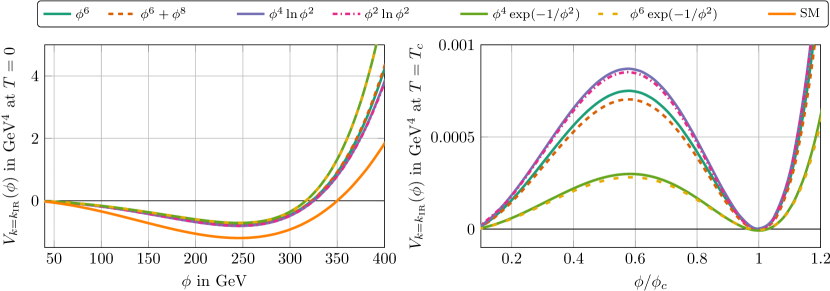
Figure 4: Effective potentials at $T=0$ (left) and $T=T_{c}$ (right). We show all modified Higgs potentials from Eq.(11) with $\Lambda=2$ TeV. The values of the coefficients at the UV scale $\Lambda$ are fixed by the requirement $\phi_{c}\approx T_{c}$, leading to $\lambda_{6}=1.2$, $\lambda_{6}=1$ with $\lambda_{8}=1.4$, $\lambda_{\ln,4}=0.89$, $\lambda_{\ln,2}=0.27$, $\lambda_{\exp,4}=23.3$, and $\lambda_{\exp,6}=27.5$.

In Fig. 3 we show the evolution of two example potentials from Eq.(11) from zero temperature to $T_{c}$, where the latter is defined as the temperature at which the two competing minima become degenerate. The latter is not distinctly apparent in Fig. 3, but becomes visible in the magnification in the right panel of Fig. 4. We also require the second minimum to be at $\phi_{c}=T_{c}$, to guarantee a sufficiently strong first-order phase transition. This way, the $\phi$ dependence of the two cases becomes comparable. A key feature already visible in this figure is that the potential with the deeper minimum at small temperature turns into the steeper potential at $T_{c}$. This is achieved by a larger value of $T_{c}$ for the potential with the deeper minimum. Note that the potentials in Fig. 3 and 4 are read off at the RG scale $k_{\text{IR}}$, which is an infrared scale where the Higgs potential and all observables are frozen out. Below this scale only convexity generating processes take place. The freeze out occurs once fluctuations of fields decouple from the RG flow because the RG scale $k$ crosses their mass-threshold. This decoupling is built into the FRG setup. We choose $k_{\text{IR}}$ to be smaller than the masses of the model, such that the exact choice of $k_{\text{IR}}$ does not matter.

In Fig. 4 we illustrate the behavior of all our modified Higgs potentials in the IR at vanishing temperature (left panel) and at the critical temperature (right panel), respectively. Note the different scales on the vertical axes. The UV scale $\Lambda$ and the respective coefficients $\lambda_{j}(\Lambda)$ are chosen such that they result in a strong first-order phase transition, $\phi_{c}/T_{c}=1$. The different potentials at zero temperature are similar to that of the Standard Model, as expected from the fact that we fix the Higgs vacuum expectation value and mass to their observed values. In particular, the minima all appear at $v=246$ GeV, and the second derivatives have to reproduce the measured Higgs mass. Nevertheless, if we fix $V_{k=k_{\text{IR}}}(0)=0$, an imprint of modified UV physics remains visible.

In the left panel of Fig. 4 we see that up to $\phi\approx 300$ GeV, all modifications we consider lead to a very similar form of the zero-temperature IR potential, if their coefficients are fixed such that $\phi_{c}/T_{c}$ is the same for all our potentials. At higher field values the different UV modifications lead to distinct field-dependence of the potential. The sizable impact of the modified microscopic action on the IR potential is due to the finite UV scale $\Lambda=2$ TeV. This is not sufficiently far above the electroweak scale for the contributions $\Delta V$ to be washed out by the RG flow.

At finite temperature, we see in the right panel of Fig. 4 that the potentials show significant deviations and the six different modifications fall into three distinct forms of the IR potential at $T_{c}$. The Standard Model is not displayed, since it exhibits a second-order phase transition with $\phi_{c}=0$. The other potentials show different sizes of the bump that separates the minima at $\phi=0$ and $\phi=\phi_{c}$. The exponential modifications show the smallest bump, while logarithmic modifications show the largest bump. The third class is given by the polynomial UV potentials, which fall in between the two other classes.

It is worth noting that the resulting IR modifications almost coincide within each class of UV potentials, i.e. , the polynomial, logarithmic, and exponential class. Although there are manifestly different UV modifications within each class, like for instance $\phi^{4}\exp(-1/\phi^{2})$ vs $\phi^{6}\exp(-1/\phi^{2})$, the resulting IR behavior appears to be dominated by the exponential dependence, and accordingly is nearly the same for the two cases – as stressed before, the two exponential cases differ from the two logarithmic cases, which are within a separate class of their own.

Comparing the two panels we observe that zero-temperature potentials with a steeper increase at larger field values turn into more shallow potentials for finite temperature near the broken vacuum. The latter corresponds to a lower barrier between the two minima. The reason for this link is that the phase transition occurs once positive thermal corrections to the mass parameter are large enough to change the extremum at $\phi=0$ from a maximum to a minimum, which then becomes degenerate with the minimum at a finite field value. For potentials with a lower zero-temperature depth — and correspondingly a more substantial slope at large $\phi$ — the corresponding critical temperature $T_{c}$ is lower. Therefore, the steepest increase towards large $\phi$ in the left panel in Fig. 4 corresponds to the smallest bump in the right panel of Fig. 4. Phrased differently: for potentials with a flatter inner region, scalar fluctuations are quantitatively more relevant. At the same time, the phase transition turns first order as soon as the scalar fluctuations dominate over the fermionic ones. This connection will become important when evaluating the prospects of the different cases with regards to detectability at the LHC.

III.2 Scale of new physics

Given a particular microscopic model containing additional degrees of freedom, the UV scale or cutoff $\Lambda$ is typically identified with the mass scale of those additional fields, below which their fluctuations are suppressed. From an EFT point of view, one correspondingly associates $\Lambda$ with the energy scale, above which new physics can appear as on-shell excitations. In turn, below $\Lambda$ the effect of new physics is only visible indirectly. Such an indirect effect would be a deviation of the Higgs potential from its form in the renormalizable Standard Model. A key aspect of this kind of approach is that an EFT description by definition comes with a region of validity, above which we will be sensitive to the actual UV completion. Hence, before we use our modified Higgs potential to link a strong first-order phase transition to the Higgs self-coupling we need to study the validity range of our description.

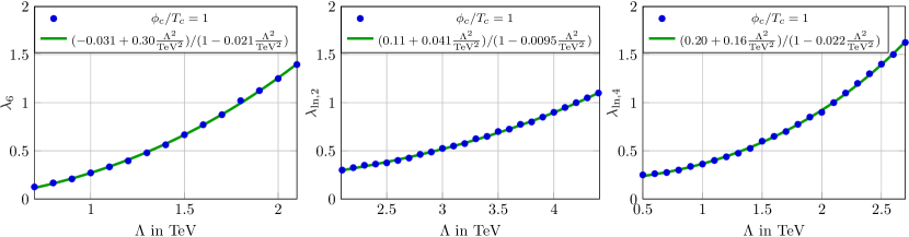
Figure 5: Coefficient $\lambda_{j}(\Lambda)$ of the dimension-6 operator $\phi^{6}/\Lambda^{2}$ (left), the modification $\Lambda^{2}\phi^{2}\ln\phi^{2}/\Lambda^{2}$ (center), and the modification $\phi^{4}\ln\phi^{2}/\Lambda^{2}$ (right) as a function of the cutoff, requiring $\phi_{c}/T_{c}=1\pm 0.05$.

Following Eq.(11) we see that an indirect measurement using an EFT-like approach is only sensitive to a combination of the scale $\Lambda$ and the (Wilson) coefficients $\lambda_{j}$. In Fig. 5 we show the correlation between $\Lambda$ and the corresponding $\lambda_{j}$ evaluated at the UV scale $\Lambda$ for a set of modified Higgs potentials, assuming a strong first-order phase transition with $\phi_{c}/T_{c}=1$. We can interpret these results as lines of constant IR physics: the running coefficient $\lambda_{j}(\Lambda)$ then describes a family of effective models defined at different scales $\Lambda$, all yielding the same IR observables. Without new physics effects, $\Delta V=0$, this corresponds to fixing $v$, $m_{H}$ and $m_{t}$ in the IR and simply evolving them toward the UV with their known RG equations. In our extended setup, the additional coefficients measure the strength of the new physics contribution, that we initialize at the UV scale $\Lambda$. We then use a corresponding parameter $\lambda_{j}$ to fix $\phi_{c}/T_{c}$ to a value of our choice. Doing so for different UV scales $\Lambda$, the coefficient $\lambda_{j}$ becomes a function of $\Lambda$.

Without running effects for the coefficients $\lambda_{j}$ the correlation between the coefficient and the UV scale would be simple. For instance, the dimension-6 Wilson coefficient would follow a parabola, $\lambda_{6}\propto\Lambda^{2}$. However, the condition on $\phi_{c}/T_{c}$ for the strong first-order phase transition is defined at energies around the Higgs VEV, while the shown values of $\lambda_{j}$ are defined in the UV. The complete correlation is well-described by a quadratic polynomial. In the case of $\lambda_{6}$, this reflects the quadratic running due to the canonical dimension. While the normalization of $\Delta V$ can be adjusted at will and the absolute values of the coefficients $\lambda_{j}$ do not carry any physical significance, the growth of these coefficients towards the ultraviolet suggests the possible onset of a strongly coupled regime.

To investigate the onset of this strongly coupled regime we fit the correlation between $\lambda_{j}$ and $\Lambda$ to a broken rational polynomial. A motivation for the particular choice of fit function in Fig. 5 is given by an approach to a power-like Landau-pole singularity. Indeed, this ansatz fits our numerical results well for the given range of UV scales. From the broken polynomial we can estimate the critical scales, where the respective models might become strongly coupled,

$$\Lambda_{6}^{\text{crit}}=7.0\,\text{TeV},\qquad\qquad\Lambda_{\ln,2}^{\text{crit}}=10\,\text{TeV},\qquad\qquad\Lambda_{\ln,4}^{\text{crit}}=6.8\,\text{TeV}\,.$$ (16)

These critical scales should be viewed as conservative estimates of the validity scale up to which our field-theory description using purely Standard-Model degrees of freedom is applicable. These estimates are of the same order of magnitude as maximum values of $\Lambda$ that lead to a first-order phase transition in studies based on mean-field arguments, see e.g. christophe_geraldine .

III.3 Baryogenesis vs Higgs self-coupling

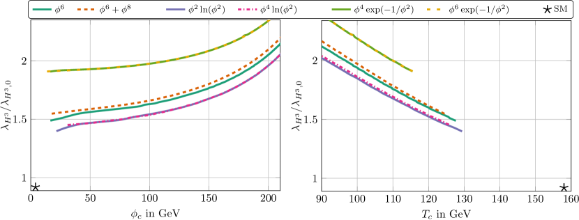
Figure 6: Modification of the self-coupling $\lambda_{H^{3}}/\lambda_{H^{3},0}$ as a function of $\phi_{c}$ (left) and $1/T_{c}$ (right) for the UV potentials given in Eq.(11). The asterisk in both plots represents the Standard Model expectation, including Coleman-Weinberg corrections, cf. Eq.(15).

After showing how a modified Higgs potential can lead to a strong first-order phase transition in Sec. III.1 and confirming that our approach is consistent in Sec. III.2, we can now explore the link between the strong first-order phase transition and the observable Higgs self-coupling. As laid out in the Introduction, the crucial question is as to whether modifications of the Higgs potential that lead to a sufficiently strong first-order phase transition for electroweak baryogenesis can be tested through the Higgs self-coupling measurement at the LHC.

Following the above discussion, the remaining question is how a value $\phi_{c}/T_{c}\approx 1$ due to the potentials given in Eq.(11) is reflected in shifted physical Higgs self-couplings $\lambda_{H^{3}}$ and $\lambda_{H^{4}}$. All new physics models are adjusted to reproduce the low-energy measurements in Eq.(12). First, we can separate the two parameters $1/T_{c}$ and $\phi_{c}$ and show their individual effects on the physical Higgs self-couplings. In Fig. 6 we first see that the two parameters contribute roughly similar amounts to an increase in the Higgs self-couplings, if we push the model towards a strong first-order phase transition. Second, we see that the individual potentials in the general class of power-series, logarithmic, and exponential potentials give essentially degenerate results. Finally, the effect on the self-couplings is the weakest for the logarithmic potential, slightly stronger for the power-law modification, and the strongest for the exponential modification.

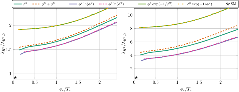
Figure 7: Modification of the self-couplings $\lambda_{H^{3}}/\lambda_{H^{3},0}$ (left) and $\lambda_{H^{4}}/\lambda_{H^{4},0}$ (right) as a function of $\phi_{c}/T_{c}$ for the UV potentials given in Eq.(11). The asterisk in the lower left of both plots represents the Standard Model expectation, including Coleman-Weinberg corrections, cf. Eq.(15).

As already observed in Sec. III.1, a steeper zero-temperature potential at large field values can be linked to a decrease in $T_{c}$. On the other hand, a steeper increase at large field values will be tied directly to larger values of the cubic and quartic Higgs self-coupling. This dependence is confirmed by Fig. 6, where potentials with smaller $T_{c}$ feature larger $\lambda_{H^{3}}$. This feature holds both within each class of potentials where we can decrease $T_{c}$ by enhancing $\Delta V$, and between different classes of potentials. This trend should be generic in that additions $\Delta V$ leading to a strong first-order transition at low $T_{c}$ will be easier to detect at the LHC.

Given that we do not see any striking effects from the individual dependence on $1/T_{c}$ and $\phi_{c}$, we study the dependence of the different Higgs potentials on the physically relevant ratio $\phi_{c}/T_{c}$. In Fig. 7, we show the modifications of both Higgs self-couplings as a function of $\phi_{c}/T_{c}$. The free model parameter along the shown line is an appropriate combination of new-physics scale $\Lambda$ and the new-physics coefficient $\lambda_{j}$. For $\phi_{c}/T_{c}\gtrsim 1$ we find a strong first-order phase transition, suitable for electroweak baryogenesis. From the location of the Standard Model point it is clear that there exists a range of modified self-couplings where the electroweak phase transition remains second order. Only for

$$\frac{\lambda_{H^{3}}}{\lambda_{H^{3},0}}\gtrsim 1.5\qquad\qquad\text{or}\qquad\qquad\frac{\lambda_{H^{4}}}{\lambda_{H^{4},0}}\gtrsim 4\,,$$ (17)

we have a chance to generate a first-order phase transition. This number should be compared to the LHC reach given in Eq.(9). We conclude that the prospects of a detectable imprint appear to be good for all models that we have studied. A strong first-order phase transition corresponding to $\phi_{c}/T_{c}>1$ can in all scenarios be achieved by further increasing the new physics contributions and thereby increasing the Higgs self-couplings. In particular, we observe that the non-perturbative modifications $\exp(-1/\phi^{2})$ lead to a significantly higher value of the Higgs self couplings at fixed $\phi_{c}/T_{c}$ and are thus easier to detect. Given that for example exponential potentials feature a minimum value of $\lambda_{H^{3}}$ significantly larger than the simple $\phi^{6}$ extension, the LHC measurement might even allow first clues to the nature of new physics, even if the corresponding scale $\Lambda$ remains out of direct reach at the LHC.

Because the curves in Fig. 7 connect an IR observable with a UV property we can link the two regimes and make two observations. First, we can start in the IR and fix $\lambda_{H^{3}}$ for different UV potentials. Here, we find that an increase in $\phi_{c}/T_{c}$ or decrease in $T_{c}$ leads to a decrease in $\lambda_{H^{4}}$ for constant $\lambda_{H^{3}}$. Alternatively, we can fix $\phi_{c}/T_{c}$ for different UV potentials and find that a decrease in $\lambda_{H^{3}}$ corresponds to a decrease also in $\lambda_{H^{4}}$ or an increase in $T_{c}$.

Finally, Fig. 8 explicitly shows the connection between the strength of the observable effect at LHC scales, measured by $\lambda_{H^{3}}/\lambda_{H^{3},0}$ and the size of the new physics contribution $\Delta V$ at the microscopic scale $\Lambda$, measured by the value of the dimensionless coefficients $\lambda_{j}$. The nature of the electroweak phase transition is encoded in the coloring of the lines. The onset of the first-order phase transition is at values that can also be read off from Fig. 7: for logarithmic modifications we find the lowest value of $\lambda_{H^{3}}/\lambda_{H^{3},0}\approx 1.4$, for the $\phi^{6}$ modification $\lambda_{H^{3}}/\lambda_{H^{3},0}\approx 1.5$, and for exponential modifications $\lambda_{H^{3}}/\lambda_{H^{3},0}\approx 1.9$. This size of all modifications can be probed in the high-luminosity run at the LHC. Importantly, the Higgs self-couplings grow continuously as a function of $\lambda_{j}$ while $\phi_{c}/T_{c}$ remains zero till the onset of the first-order phase transition and only then starts to grow continuously.

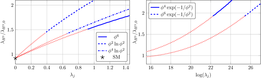
Figure 8: Modification of the self-coupling $\lambda_{H^{3}}/\lambda_{H^{3},0}$ as a function of the coefficients $\lambda_{j}$ from the different UV potentials given in Eq.(11). Blue lines represent first-order phase transitions and red dotted lines second-order phase transitions. The cutoff is $\Lambda=2$ TeV.

IV Outlook

Higgs pair production or the measurement of the Higgs self coupling is an extraordinarily interesting LHC analysis. We find that it is well motivated by modified Higgs potentials which allow for a strong first-order electroweak phase transition and hence an explanation of the observed matter vs anti-matter asymmetry. We have studied a wide range of such modifications to the Higgs potential, especially potentials that cannot be expanded as an effective field theory. We used the functional renormalization group to describe the dependence on the field value $\phi$ and on the temperature $T$. For all classes of potentials considered here, there exists an appropriate choice of model parameters, for which the phase transition is of first order and sufficiently strong, $\phi_{c}/T_{c}\gtrsim 1$.

Our numerical analysis indicates that the requirement $\phi_{c}/T_{c}=1$ corresponds to a critical scale of the order of 10 TeV for all our potentials, where the potentials become strongly coupled. Below this scale we can rely on our assumed potentials to describe LHC signals. We then found that a strong first-order phase transition universally predicts an enhancement of the Higgs self-couplings $\lambda_{H^{3}}\gtrsim 1.5\lambda_{H^{3},0}$ and $\lambda_{H^{4}}\gtrsim 4\lambda_{H^{4},0}$. Extending earlier studies, we systematically established this connection between a first-order transition and a measurable deviation of the Higgs self couplings, employing a method that can describe systems with multiple physical scales in a controlled manner. While it might be possible that a new physics model features a strong first-order transition with all effects on $\lambda_{H^{3/4}}$ canceling accidentally Noble , none of our examples falls into this class. We conclude that a measurement of the Higgs self-couplings at the LHC indeed serves as an indirect probe of a first-order phase transition and thus of electroweak baryogenesis in generic setups.

On the other hand, we observed that it is possible to obtain large deviations in the Higgs self-interactions for our class of non-perturbative potentials without the condition $\phi_{c}/T_{c}\geq 1$ being fulfilled. For example with an exponential modification of the Higgs potential the physical Higgs self-coupling reaches $\lambda_{H^{3}}\approx 1.9\lambda_{H^{3},0}$ already significantly below $\phi_{c}/T_{c}=1$. On the theoretical side, a quantitative upgrade of our analysis includes, but is not limited to, a full treatment of the weak gauge sector as well as improvements in our treatment of the Yukawa sector, which might result in quantitative changes of the order of 10 %, cf. Gies:2017zwf . An as precise as possible measurement of the triple-Higgs interaction is clearly desirable. For instance a $20\%$ measurement of a relatively small modification of $\lambda_{H^{3}}/\lambda_{H^{3},0}$ could exclude such exponential potentials as sources of electroweak baryogenesis. Such an actual measurement could therefore provide valuable hints guiding theoretical studies of interesting extended Higgs models.

Acknowledgments

We thank R. Sondenheimer for insightful discussions. MR acknowledges funding from IMPRS-PTFS and is grateful to the DFG research training group GRK 1523 at TPI Jena for hospitality. JMP is supported by the Helmholtz Alliance HA216/EMMI and by ERC-AdG-290623. AE is supported by an Emmy-Noether grant of the DFG under Ei-1037/1 and an Emmy-Noether visiting fellowship at the Perimeter Institute for Theoretical Physics. This work is part of and supported by the DFG Collaborative Research Centre ”SFB 1225 (ISOQUANT)”.

Appendix A Flow equations

The set of couplings in our setup consists of the $SU(3)$ coupling $g_{3}$, a fiducial coupling $g_{F}$ that simulates the $SU(2)$ and the $U(1)$ sector, the top-Yukawa coupling $y_{t}$, and the full Higgs potential $V(\phi)$ our_paper . For the $SU(3)$ coupling it suffices to consider one-loop running, since higher-order or threshold corrections have little impact on the phase transition. The one-loop beta function is given by

$$\beta_{g_{3}}=-\frac{g_{3}^{3}}{(4\pi)^{2}}\left(11-\frac{2}{3}n_{f}\right)\,,$$ (18)

with $n_{f}=6$. We fix the $SU(3)$ coupling through $g_{3}(1\,\text{TeV})=1.06$, so the scale-dependent $SU(3)$ coupling is known analytically. We approximate its temperature dependence by replacing $k\rightarrow\sqrt{k^{2}+\pi\,T^{2}}$,

$$g_{3}(k,T)=\left(\frac{7}{8\pi^{2}}\ln\frac{\sqrt{k^{2}+\pi T^{2}}}{1\,\text{TeV}}+\frac{1}{1.06^{2}}\right)^{-1/2}\,.$$ (19)

The logarithmic running of the $U(1)$ and $SU(2)$ couplings is sufficiently slow to be negligible for our purpose our_paper . We model it as a fiducial coupling $g_{F}$ that is a constant as a function of the RG scale and thus also a constant as a function of the temperature. At finite temperature, this simplified treatment must be ameliorated by a thermal mass generated by fluctuations from the electroweak sector. According to the high-$T$ expansion of the one-loop thermal potential it is given by

$$V_{\text{thermal mass}}(\phi,T)=\frac{1}{16}\left(3g^{2}+{g^{\prime}}^{2}\right)\;\frac{T^{2}\phi^{2}}{2}\,,$$ (20)

where $g=0.65$ and $g^{\prime}=0.36$ are the $SU(2)$ and $U(1)$ gauge couplings, respectively.

To derive beta functions for the Higgs potential and the top-Yukawa coupling we introduce the renormalized dimensionless field $\rho$ and the dimensionless potential $u$

$$\rho=\frac{\phi^{2}}{2k^{2}Z_{\phi}}\qquad\qquad\qquad u(\rho)=\frac{V(\phi(\rho))}{k^{4}}\,.$$ (21)

The wave function renormalizations of the fields appear in the beta functions only via their anomalous dimension

$$\eta_{\phi}=-\frac{\mathrm{d}\log Z_{\phi}}{\mathrm{d}\log k}\qquad\qquad\qquad\eta_{\psi}=-\frac{\mathrm{d}\log Z_{\psi}}{\mathrm{d}\log k}\,.$$ (22)

Written in terms of threshold functions, the beta function for the top Yukawa coupling agrees with that from Refs. our_paper ; Gies:2013fua , see, e.g.  Eq.(C8) of Ref. our_paper . However, we use a spatial regulator as described below and temperature-dependent threshold functions. The spatial regulator changes some prefactors, which is compensated by the different definition of the threshold functions. The beta function is given by

$$\frac{\mathrm{d}y_{t}^{2}}{\mathrm{d}\log k}={} y_{t}^{2}\left(\eta_{\phi}+2\eta_{\psi}\right)-\frac{y_{t}^{4}}{\pi^{2}}\left(3\kappa u^{\prime\prime}(\kappa)+2\kappa^{2}u^{(3)}(\kappa)\right)l_{1,2}^{(FB)4}\left(\kappa y_{t}^{2},u^{\prime}(\kappa)+2\kappa u^{\prime\prime}(\kappa);\eta_{\psi},\eta_{\phi};T\right)$$

$$+\frac{y_{t}^{4}}{2\pi^{2}}\left(l_{1,1}^{(FB)4}\left(\kappa y_{t}^{2},u^{\prime}(\kappa)+2\kappa u^{\prime\prime}(\kappa);\eta_{\psi},\eta_{\phi};T\right)\right.$$

$$\left.\hskip 56.9055pt-2\kappa y_{t}^{2}\,l_{2,1}^{(FB)4}\left(\kappa y_{t}^{2},u^{\prime}(\kappa)+2\kappa u^{\prime\prime}(\kappa);\eta_{\psi},\eta_{\phi};T\right)\right)$$

$$+\frac{3}{\pi^{2}}\frac{\left(N_{c}^{2}-1\right)}{2N_{c}}g_{3}^{2}y_{t}^{2}\left(2\kappa y_{t}^{2}\,l_{2,1}^{(FB)4}(\kappa y_{t}^{2},0;\eta_{\psi},\eta_{A};T)-l_{1,1}^{(FB)4}(\kappa y_{t}^{2},0;\eta_{\psi},\eta_{A};T)\right)$$

$$-\frac{c_{y}g_{F}^{2}y_{t}^{2}}{16\pi^{2}\left(1+\left(\frac{80}{246}\right)^{2}\kappa\right)}\,,$$ (23)

where $c_{y}=97/30$ and $N_{c}=3$. It depends on the position of the renormalized dimensionless minimum $\kappa$ of the potential, the anomalous dimensions of the fields, as well as on regulator-dependent threshold functions specified below. Here, we have employed the same projection scheme onto the Yukawa flow as in our_paper for reasons of comparison. In principle, there exists an improved scheme Pawlowski:2014zaa more adequately capturing higher-order contributions to the Yukawa flow for the present model Gies:2017zwf , possibly improving the fixing of initial conditions on the 5% level. In either case, working in the symmetric regime with $\kappa=0$ and neglecting the additional $\eta$ dependence in the threshold functions reproduces the universal one-loop beta functions, as it should.

The beta function for the Higgs potential at vanishing temperature has been computed in Ref. our_paper ; Gies:2013fua , see, e.g.  Eq.(E1) of Ref. our_paper . As for the beta function of the Yukawa coupling, the present finite temperature beta function for the Higgs potential agrees with the $T=0$ one in terms of the threshold functions

$$\frac{\mathrm{d}u(\rho)}{\mathrm{d}\log k}={} -4u(\rho)+(2+\eta_{\phi})\rho\,u^{\prime}(\rho)$$

$$+\frac{1}{4\pi^{2}}\left(l_{0}^{(B)4}\left(u^{\prime}(\rho)+2\rho\,u^{\prime\prime}(\rho);\eta_{\phi};T\right)-4N_{c}l_{0}^{(F)4}(y_{t}^{2}\rho;\eta_{\psi};T)\right)+\frac{c_{l}}{2\pi^{2}\left(1+\frac{g_{F}^{2}\rho}{2}\right)}\,,$$ (24)

where $c_{l}=9/16$ and again $N_{c}=3$.

Finally, we need expressions for the anomalous dimensions of the Higgs field and the top-quark: the first two terms in Eq.(A) are integral parts of the universal one-loop contribution. In terms of the threshold functions the anomalous dimension of the top quark agrees with the $T=0$ one in Eq.(C8) of Ref. our_paper , and the anomalous dimension of the scalar field has the same form as in Eq.(16) of Ref. Gies:2013fua . With the thermal threshold functions of the present work this means

$$\eta_{\phi}={} \frac{2}{3\pi^{2}}N_{c}y_{t}^{2}\left(m_{4}^{(F)4}(\kappa y_{t}^{2};\eta_{\psi};T)-\kappa y_{t}^{2}m_{2}^{(F)4}(\kappa y_{t}^{2};\eta_{\psi};T)\right)$$

$$+\frac{1}{3\pi^{2}}\kappa\left(3u^{\prime\prime}(\kappa)+2\kappa u^{(3)}(\kappa)\right)^{2}m_{4}^{(B)4}\left(u^{\prime}(\kappa)+2\kappa u^{\prime\prime}(\kappa);\eta_{\phi};T\right)\,,$$

$$\eta_{\psi}={} \frac{1}{6\pi^{2}}y_{t}^{2}\,m_{1,2}^{(FB)4}\left(\kappa y_{t}^{2},u^{\prime}(\kappa)+2\kappa u^{\prime\prime}(\kappa);\eta_{\phi};T\right)$$

$$+\frac{1}{2\pi^{2}}\frac{\left(N_{c}^{2}-1\right)}{2N_{c}}g_{3}^{2}\left(m_{1,2}^{(FB)4}(\kappa y_{t}^{2},0;\eta_{\psi},0;T)-\tilde{m}_{1,1}^{(FB)4}(\kappa y_{t}^{2},0;\eta_{\psi},0;T)\right)\,.$$ (25)

The beta functions found above are expressed in terms of regulator-dependent and temperature-dependent threshold functions. Here we provide explicit analytic results for these threshold functions for one specific regulator. The analyticity of the threshold function is rooted in the use of a Litim-type regulator flat-reg that only regularizes the spatial momenta. The dimensionless bosonic and fermionic propagators are regularized as

$$G_{\phi}(\omega_{n}^{2},{\vec{p}\,}^{2},m_{\phi}^{2})=\left(\omega_{n}^{2}+{\vec{p}\,}^{2}/k^{2}(1+r_{B}({\vec{p}\,}^{2}/k^{2}))+m_{\phi}^{2}\right)^{-1}\,,$$

$$G_{\psi}(\nu_{n}^{2},{\vec{p}\,}^{2},m_{\psi}^{2})=\left(\nu_{n}^{2}+{\vec{p}\,}^{2}/k^{2}(1+r_{F}({\vec{p}\,}^{2}/k^{2}))+m_{\psi}^{2}\right)^{-1}\,,$$ (26)

with the bosonic Matsubara frequency $\omega_{n}=2\pi nT/k$ and the fermionic Matsubara frequency $\nu_{n}=2\pi(n+\frac{1}{2})T/k$. Note that $m_{\phi}$ and $m_{\psi}$ are dimensionless mass-like arguments. The bosonic and fermionic regulator shape functions read flat-reg

$$r_{B}(x)=\left(x^{-1}-1\right)\Theta(1-x)\,,\qquad\qquad r_{F}(x)=\left(x^{-1/2}-1\right)\Theta(1-x)\,,$$ (27)

where $x={\vec{p}\,}^{2}/k^{2}$. In the following, we express the threshold functions in terms of the bosonic and fermionic distribution functions,

$$n_{F,B}(m_{\psi,\phi}^{2},T)=\left(\exp\left(\frac{k}{T}\sqrt{1+m_{\psi,\phi}^{2}}\right)\mp 1\right)^{-1}\;.$$ (28)

The set of threshold functions we need in our calculation includes

$$l_{0}^{(B)d}(m_{\phi}^{2};\eta_{\phi};T)={} \frac{2}{d-1}\left(1-\frac{\eta_{\phi}}{d+1}\right)\mathcal{B}_{(1)}(m_{\phi}^{2};T)\,,$$

$$l_{0}^{(F)d}(m_{\psi}^{2};\eta_{\psi};T)={} \frac{2}{d-1}\left(1-\frac{\eta_{\psi}}{d}\right)\mathcal{F}_{(1)}(m_{\psi}^{2};T)\,,$$

$$l_{n,m}^{(FB)d}(m_{\psi}^{2},m_{\phi}^{2};\eta_{\psi},\eta_{\phi};T)={} \frac{2}{d-1}\left(n\left(1-\frac{\eta_{\psi}}{d}\right)\mathcal{FB}_{(n+1,m)}(m_{\psi}^{2},m_{\phi}^{2};T)\right.$$

$$\left.\hskip 48.36958pt+m\left(1-\frac{\eta_{\phi}}{d+1}\right)\mathcal{FB}_{(n,m+1)}(m_{\psi}^{2},m_{\phi}^{2};T)\right)\,,$$

$$m_{4}^{(B)d}\left(m_{\phi}^{2};\eta_{\phi};T\right) =\mathcal{B}_{(4)}(m_{\phi}^{2};T)\,,$$

$$m_{2}^{(F)d}(m_{\psi}^{2};T) =\mathcal{F}_{(4)}(m_{\psi}^{2};T)\,,$$

$$m_{4}^{(F)d}(m_{\psi}^{2};\eta_{\psi};T) =\mathcal{F}_{(4)}(m_{\psi}^{2};T)+\frac{1-\eta_{\psi}}{d-3}\mathcal{F}_{(3)}(m_{\psi}^{2};T)-\frac{1}{2}\left(\frac{1-\eta_{\psi}}{d-3}+\frac{1}{2}\right)\mathcal{F}_{(2)}(m_{\psi}^{2};T)\,,$$

$$m_{1,2}^{(FB)d}(m_{\psi}^{2},m_{\phi}^{2};\eta_{\psi},\eta_{\phi};T) =\left(1-\frac{\eta_{\phi}}{d}\right)\mathcal{FB}_{(1,2)}(m_{\psi}^{2},m_{\phi}^{2};T)\,,$$

$$\tilde{m}_{1,1}^{(FB)d}(m_{\psi}^{2},m_{\phi}^{2};\eta_{\psi},\eta_{\phi};T) =\frac{2}{d-2}\left(\left(1-\frac{\eta_{\phi}}{d}\right)\mathcal{FB}_{(1,2)}(m_{\psi}^{2},m_{\phi}^{2};T)\right.$$

$$\qquad\qquad+\left(1-\frac{\eta_{\psi}}{d-1}\right)\mathcal{FB}_{(2,1)}(m_{\psi}^{2},m_{\phi}^{2};T)$$

$$\qquad\qquad\left.-\frac{1}{2}\left(1-\frac{\eta_{\psi}}{d-1}\right)\mathcal{FB}_{(1,1)}(m_{\psi}^{2},m_{\phi}^{2};T)\right)\,.$$ (29)

All threshold functions are expressed in terms of

$$\mathcal{F}_{(1)}(m_{\psi}^{2};T) =\frac{T}{k}\sum_{n\in\mathbb{Z}}G_{\psi}(\nu_{n},m_{\psi}^{2})\,,$$

$$\mathcal{B}_{(1)}(m_{\phi}^{2};T) =\frac{T}{k}\sum_{n\in\mathbb{Z}}G_{\phi}(\omega_{n},m_{\phi}^{2})\,,$$

$$\mathcal{FB}_{(1,1)}(m_{\psi}^{2},m_{\phi}^{2};T) =\frac{T}{k}\sum_{n\in\mathbb{Z}}G_{\psi}(\nu_{n},m_{\psi}^{2})G_{\phi}(\omega_{n},m_{\phi}^{2})\,.$$ (30)

At finite temperature for the flat regulators in Eq.(27) they are given by

$$\mathcal{F}_{(1)}(m_{\psi}^{2};T)={} \frac{1}{\sqrt{1+m_{\psi}^{2}}}\left(\frac{1}{2}-n_{F}(m_{\psi}^{2},T)\right)\,,$$

$$\mathcal{B}_{(1)}(m_{\phi}^{2};T)={} \frac{1}{\sqrt{1+m_{\phi}^{2}}}\left(\frac{1}{2}+n_{B}(m_{\phi}^{2},T)\right)\,,$$

$$\mathcal{FB}_{(1,1)}(m_{\psi}^{2},m_{\phi}^{2};T)={} \Bigg{[}\frac{\frac{1}{2}+n_{B}(m_{\phi}^{2},T)}{2\sqrt{1+m_{\phi}^{2}}}\left(\left(m_{\psi}^{2}+1-\left(i\pi T/k+\sqrt{1+m_{\phi}^{2}}\right)^{2}\right)^{-1}\right.$$

$$\hskip 99.58464pt\left.+\left(m_{\psi}^{2}+1-\left(i\pi T/k-\sqrt{1+m_{\phi}^{2}}\right)^{2}\right)^{-1}\right)$$

$$\,\,+\frac{\frac{1}{2}-n_{F}(m_{\psi}^{2},T)}{2\sqrt{1+m_{\psi}^{2}}}\left(\left(m_{\phi}^{2}+1-\left(i\pi T/k+\sqrt{1+m_{\psi}^{2}}\right)^{2}\right)^{-1}\right.$$

$$\hskip 99.58464pt+\left.\left(m_{\phi}^{2}+1-\left(i\pi T/k-\sqrt{1+m_{\psi}^{2}}\right)^{2}\right)^{-1}\right)\Bigg{]}\,.$$ (31)

They obey the relations

$$\frac{\partial\mathcal{F}_{(n)}}{\partial m_{\psi}^{2}} =-n\mathcal{F}_{(n+1)}\,,\qquad\qquad\qquad \frac{\partial\mathcal{B}_{(n)}}{\partial m_{\phi}^{2}} =-n\mathcal{B}_{(n+1)}\,,$$

$$\frac{\partial\mathcal{FB}_{(m,n)}}{\partial m_{\psi}^{2}} =-m\mathcal{FB}_{(m+1,n)}\,,\qquad\qquad\qquad \frac{\partial\mathcal{FB}_{(m,n)}}{\partial m_{\phi}^{2}} =-n\mathcal{FB}_{(m,n+1)}\,.$$ (32)

The notation and the threshold functions agree with Ref. Pawlowski:2014zaa . Note, that the $T\to 0$ limit of the threshold functions does not agree with the ones given in Ref. Gies:2013fua , since we use a spatial regulator while Ref. Gies:2013fua uses a covariant regulator. This concludes the list of threshold functions and relations necessary in order to numerically evaluate the previously given beta functions.

Appendix B Grid approach and benchmarking

We solve the functional differential equation for the Higgs potential, Eq.(A), using a grid code. This means that the potential $u(\rho)$ and its derivative $u^{\prime}(\rho)$ are discretized on a grid in the field invariant $\rho$. The discretization converts the partial differential equation for $u(\rho)$ into a large set of coupled ordinary differential equations. The grid code has to manage a numerical integration from $k=\Lambda$, where we initialize the flow, down to $k=k_{\text{IR}}\approx 100$ GeV. At this IR value all physical relevant quantities are frozen out and only convexity-generating processes take place.

The grid code also has to cover a large range of values in the scalar field $0\leq\phi\leq c\Lambda$, where we typically choose $c=\mathcal{O}(1\dots 10)$. To resolve both, large field values and the minimum of the potential at small field values, we employ an exponential distribution of the grid points $\rho_{i}=\phi_{i}^{2}/2$ with $i\in{0,\ldots,N-1}$ according to

$$\rho_{i}=\rho_{\text{a}}+\frac{\exp\left(\frac{i}{c_{\text{grid}}}\right)-1}{\exp\left(\frac{(N-1)}{c_{\text{grid}}}\right)}\rho_{\text{b}}\,,$$ (33)

where $N$ is the number of grid points, $c_{\text{grid}}$ a grid parameter that governs the distributions of the grid points, and $\rho_{\text{a}}$ and $\rho_{\text{b}}$ the smallest and largest included field value, respectively.

We introduce a grid for the potential $u(\rho_{i})$ as well as for the derivative of the potential $u^{\prime}(\rho_{i})$, and we match the second and third derivative of the potential in between the grid points grid-code . This is augmented by a differential equation for the top-Yukawa coupling, while the $SU(3)$ coupling is already integrated out and the fiducial coupling for $SU(2)$ and $U(1)$ remains constant. Consequently, we obtain a system of $2N+1$ coupled differential equations for a grid consisting of $N$ points, which is solved with an iterative Runge-Kutta-Fehlberg method with an adaptive step size.

At the IR scale and at vanishing temperature, we match the output of the grid code with the physically known observables, see Eq.(12). This is implemented on the level of the variables of the grid code and in particular we demand that the errors fulfill $\Delta\rho_{\text{min}}\leq 20$ GeV², $\Delta\lambda_{4}\leq 0.002$ and $\Delta y_{t}\leq 0.0014$. Expressed in the quantities of Eq.(12) these errors correspond to $\Delta v\leq 0.08$ GeV, $\Delta m_{H}\leq 0.28$ GeV, and $\Delta m_{t}\leq 0.23$ GeV. It is important to determine the vacuum expectation value more precisely since its error directly influences the error on the Higgs and the top mass.

To achieve this precision we tune the parameters $\mu$, $\lambda_{4}$ and $y_{t}$ at the UV scale, which is done by a secant method in $\mu$ and a two-dimensional bisection method in $\lambda_{4}$ and $y_{t}$ . The grid code might exhibit other systematic errors and in particular the measurement of the Higgs mass is challenging since it is related to the second derivative of the potential. Hence we conservatively estimate the total accuracy of the IR values with

$$\Delta v\leq 0.2\ \text{GeV}\,,\qquad\qquad\Delta m_{H}\leq 1.5\ \text{GeV}\,,\qquad\qquad\Delta m_{t}\leq 0.5\ \text{GeV}\,.$$ (34)

The tuning process is performed at vanishing temperature and the tuned initial values are subsequently used as initial values for all finite-temperature computations. For each temperature we initialize the flow in this way and determine the position of the minimum at the IR scale $k_{\text{IR}}$. The critical temperature is obtained with a bisection method where we demand an accuracy of $\Delta T_{c}\leq 0.2$ MeV. This high accuracy is necessary for a precise value of $\phi_{c}$, which is in turn given by the position of the minimum at the temperature just below $T_{c}$. From the grid code, it is difficult to get a clear signature distinguishing between second-order phase transitions and weak first-order phase transitions. Within our numerical accuracy, a reliable distinguishing signature is not available for $\phi_{c}\lesssim 20$ GeV. For finite temperature computations we slightly increase the number of grid points, since the exponential functions in the bosonic and fermionic distribution functions make these computations technically more challenging.

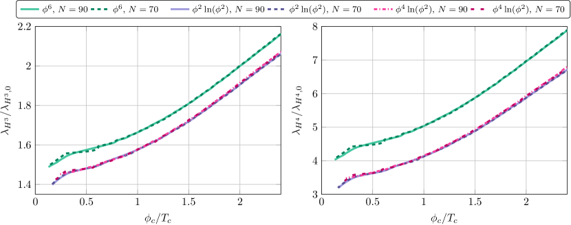
Figure 9: Modification of the self-couplings $\lambda_{H^{3}}/\lambda_{H^{3},0}$ (left) and $\lambda_{H^{4}}/\lambda_{H^{4},0}$ (right) as a function of $\phi_{c}/T_{c}$ for polynomial and logarithmic modifications of the UV potentials, cf. Eq.(11). We compare results for $N=70$ and $N=90$ grid points.

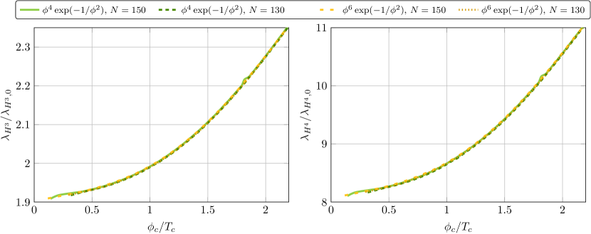
Figure 10: Modification of the self-couplings $\lambda_{H^{3}}/\lambda_{H^{3},0}$ (left) and $\lambda_{H^{4}}/\lambda_{H^{4},0}$ (right) as a function of $\phi_{c}/T_{c}$ for exponential modifications of the UV potentials, cf. Eq.(11). We compare results for $N=130$ and $N=150$ grid points.

We test our numerical results by first comparing the observables for two different numbers of grid points. The necessary number varies with our choice of cutoff and the modification of the Higgs potential. For example, more grid points are necessary for the exponential modifications of the potential. For polynomial and logarithmic modifications and a cutoff $\Lambda=2$ TeV, we use typically $N=90$ grid points, while for exponential modifications with the same cutoff we use $N=150$ grid points. In Fig. 9 we display results for polynomial and logarithmic modifications. In particular we show the correlation between the strength of first-order phase transition and the Higgs-self couplings. In Fig. 10 we show the same correlation but for exponential modifications and for $N=130$ and for $N=150$ grid points. The results for $N=90$ and for $N=150$ are identical with those displayed in Fig. 7.

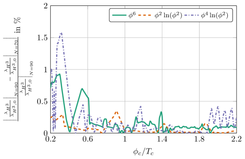
Figure 11: Relative change of $\lambda_{H^{3}}/\lambda_{H^{3},0}$ with different numbers of grid points as a function of $\phi_{c}/T_{c}$ for polynomial and logarithmic modifications of the UV potentials, cf. Eq.(11). In the regime of interest of $\phi_{c}/T_{c}\geq 1$, the relative difference between $N=70$ and $N=90$ is in the sub-percent regime, $\leq 0.5\%$.

To make our analysis more quantitative we also display the relative change of the correlation for polynomial and logarithmic modifications in Fig. 11. The results do not change significantly when we increase the number of grid points. In case of polynomial and logarithmic modifications the amount of wiggles in the region of a weak first-order phase transition, which originates from numerical uncertainties, is further reduced. In the region of a weak first-order phase transition we have a relative change of less than 2%, while in the region of a strong first-order phase transition we have a relative change of less than 0.5%. This is sufficient for our analysis, since we are only interested in the latter case. In case of the exponential modifications the change is hardly visible. The relative change is globally less than 0.02%. These results illustrate that our findings are indeed numerically stable.

Finally, we can compare our functional renormalization group results to other methods, for instance to the mean-field-like methods of Ref. christophe_geraldine . To perform a meaningful comparison, we have to take into account the slightly different setup: while we modify the microscopic potential, Ref. christophe_geraldine implements the modifications directly at the level of the effective potential. This means that in our setup a $\phi^{6}$ modification of the microscopic potential generates finite higher-order modifications through quantum fluctuations, which in the weak coupling regime are similar to the one-loop determinant. These additional terms do not appear in Ref. christophe_geraldine .

For our comparison we therefore adjust the parameter $\lambda_{6}$ such that the $T=0$ effective potentials of both setups agree. Due to the impact of quantum fluctuations, different values of $\Lambda$ require slightly different initial conditions for $\lambda_{6}$ in our setup. With a cutoff $\Lambda=1$ TeV it turns out that this is the case for $\lambda_{6}\approx 0.21$, while for a cutoff $\Lambda=0.6$ TeV we find $\lambda_{6}\approx 0.19$. The difference in values of $\lambda_{6}$ is accounted for by the RG flow between the two choices of cutoff scale. With these values we can then compare $T_{c}$ and $\phi_{c}/T_{c}$. As expected, we indeed find good qualitative agreement. For instance, for $\Lambda=0.6$ TeV we find $\phi_{c}/T_{c}=2.7$ and $T_{c}=83$ GeV vs $\phi_{c}/T_{c}=2.8$ and $T_{c}=75$ GeV from Ref. christophe_geraldine . We emphasize that a more precise agreement cannot be expected: the modification of the microscopic and the effective Higgs potential are necessarily different, as our setup accounts for quantum fluctuations, in particular affecting $\lambda_{6}$ between the microscopic scale and the IR.

References

- (1) A. D. Sakharov, Pisma Zh. Eksp. Teor. Fiz. 5, 32 (1967) [JETP Lett. 5, 24 (1967)] [Sov. Phys. Usp. 34, 392 (1991)] [Usp. Fiz. Nauk 161, 61 (1991)]; V. A. Kuzmin, V. A. Rubakov and M. E. Shaposhnikov, Phys. Lett. 155B, 36 (1985); V. A. Rubakov and M. E. Shaposhnikov, Usp. Fiz. Nauk 166, 493 (1996) [Phys. Usp. 39, 461 (1996)] [hep-ph/9603208]; M. Trodden, Rev. Mod. Phys. 71, 1463 (1999) [hep-ph/9803479].
- (2) M. Sher, Phys. Rept. 179, 273 (1989); A. G. Cohen, D. B. Kaplan and A. E. Nelson, Ann. Rev. Nucl. Part. Sci. 43, 27 (1993) [hep-ph/9302210]; J. M. Cline, [hep-ph/0609145]; D. E. Morrissey and M. J. Ramsey-Musolf, New J. Phys. 14, 125003 (2012) [arXiv:1206.2942 [hep-ph]]; T. Konstandin, Phys. Usp. 56, 747 (2013) [Usp. Fiz. Nauk 183, 785 (2013)] [arXiv:1302.6713 [hep-ph]].
- (3) M. E. Shaposhnikov, Nucl. Phys. B 287, 757 (1987); Nucl. Phys. B 299, 797 (1988).
- (4) Z. Fodor, J. Hein, K. Jansen, A. Jaster and I. Montvay, Nucl. Phys. B 439, 147 (1995) [hep-lat/9409017]; W. Buchmuller, Z. Fodor and A. Hebecker, Nucl. Phys. B 447, 317 (1995) [hep-ph/9502321]; K. Kajantie, M. Laine, K. Rummukainen and M. E. Shaposhnikov, Phys. Rev. Lett. 77, 2887 (1996) [hep-ph/9605288]; K. Rummukainen, M. Tsypin, K. Kajantie, M. Laine and M. E. Shaposhnikov, Nucl. Phys. B 532, 283 (1998) [hep-lat/9805013]; F. Csikor, Z. Fodor and J. Heitger, Phys. Rev. Lett. 82, 21 (1999) [hep-ph/9809291].
- (5) M. E. Shaposhnikov, Phys. Lett. B 277, 324 (1992) Erratum: [Phys. Lett. B 282, 483 (1992)].
- (6) X. m. Zhang, Phys. Rev. D 47, 3065 (1993) [hep-ph/9301277]; X. Zhang, B. L. Young and S. K. Lee, Phys. Rev. D 51, 5327 (1995) [hep-ph/9406322].
- (7) C. Grojean, G. Servant and J. D. Wells, Phys. Rev. D 71, 036001 (2005) [hep-ph/0407019].
- (8) S. Kanemura, Y. Okada and E. Senaha, Phys. Lett. B 606, 361 (2005) [hep-ph/0411354]; F. P. Huang, P. H. Gu, P. F. Yin, Z. H. Yu and X. Zhang, Phys. Rev. D 93, no. 10, 103515 (2016) [arXiv:1511.03969 [hep-ph]]; P. Huang, A. Joglekar, B. Li and C. E. M. Wagner, Phys. Rev. D 93, no. 5, 055049 (2016) [arXiv:1512.00068 [hep-ph]]; A. Kobakhidze, L. Wu and J. Yue, JHEP 1604, 011 (2016) [arXiv:1512.08922 [hep-ph]]; Q. H. Cao, G. Li, B. Yan, D. M. Zhang and H. Zhang, Phys. Rev. D 96, no. 9, 095031 (2017) [arXiv:1611.09336 [hep-ph]]; D. Curtin, P. Meade and H. Ramani, arXiv:1612.00466 [hep-ph]; X. Gan, A. J. Long and L. T. Wang, Phys. Rev. D 96, no. 11, 115018 (2017) [arXiv:1708.03061 [hep-ph]]; Q. H. Cao, F. P. Huang, K. P. Xie and X. Zhang, Chin. Phys. C 42, no. 2, 023103 (2018) [arXiv:1708.04737 [hep-ph]]; B. Jain, S. J. Lee and M. Son, arXiv:1709.03232 [hep-ph].
- (9) A. Noble and M. Perelstein, Phys. Rev. D 78, 063518 (2008) [arXiv:0711.3018 [hep-ph]].
- (10) U. Baur, T. Plehn and D. L. Rainwater, Phys. Rev. Lett. 89, 151801 (2002) [hep-ph/0206024]; Phys. Rev. D 67, 033003 (2003) [hep-ph/0211224].
- (11) for an analysis of the Higgs-gauge sector based on the full Run I data set see A. Butter, O. J. P. Eboli, J. Gonzalez-Fraile, M. C. Gonzalez-Garcia, T. Plehn and M. Rauch, JHEP 1607, 152 (2016) [arXiv:1604.03105 [hep-ph]].
- (12) K. Holland and J. Kuti, Nucl. Phys. Proc. Suppl. 129, 765 (2004) [hep-lat/0308020]; K. Holland, Nucl. Phys. Proc. Suppl. 140, 155 (2005) [hep-lat/0409112]; J. R. Espinosa, T. Konstandin and F. Riva, Nucl. Phys. B 854, 592 (2012) [arXiv:1107.5441 [hep-ph]].
- (13) H. Gies, C. Gneiting and R. Sondenheimer, Phys. Rev. D 89, no. 4, 045012 (2014) [arXiv:1308.5075 [hep-ph]]. H. Gies and R. Sondenheimer, Eur. Phys. J. C 75, no. 2, 68 (2015) [arXiv:1407.8124 [hep-ph]]; Phil. Trans. Roy. Soc. Lond. 376, no. 2114, 20170120 (2018) [arXiv:1708.04305 [hep-ph]].
- (14) J. Borchardt, H. Gies and R. Sondenheimer, Eur. Phys. J. C 76, no. 8, 472 (2016) [arXiv:1603.05861 [hep-ph]].
- (15) R. Sondenheimer, arXiv:1711.00065 [hep-ph].
- (16) O. Akerlund and P. de Forcrand, Phys. Rev. D 93, no. 3, 035015 (2016) [arXiv:1508.07959 [hep-lat]]; D. Y.-J. Chu, K. Jansen, B. Knippschild and C.-J. D. Lin, EPJ Web Conf. 175, 08017 (2018) [arXiv:1710.09737 [hep-lat]].
- (17) O. Akerlund, P. de Forcrand and J. Steinbauer, PoS LATTICE 2015, 229 (2016) [arXiv:1511.03867 [hep-lat]].
- (18) C. Wetterich, Phys. Lett. B 301, 90 (1993).
- (19) for an overview see e.g. J. Berges, N. Tetradis and C. Wetterich, Phys. Rept. 363, 223 (2002); J. M. Pawlowski, Annals Phys. 322, 2831 (2007); H. Gies, Lect. Notes Phys. 852, 287 (2012); J. Braun, J. Phys. G 39, 033001 (2012).
- (20) I. V. Krive and A. D. Linde, Nucl. Phys. B 117, 265 (1976).
- (21) M. Lindner, Z. Phys. C 31, 295 (1986).
- (22) D. Buttazzo, G. Degrassi, P. P. Giardino, G. F. Giudice, F. Sala, A. Salvio and A. Strumia, JHEP 1312, 089 (2013) [arXiv:1307.3536 [hep-ph]].
- (23) A. Eichhorn, H. Gies, J. Jaeckel, T. Plehn, M. M. Scherer and R. Sondenheimer, JHEP 1504, 022 (2015) [arXiv:1501.02812 [hep-ph]].
- (24) Z. Fodor, K. Holland, J. Kuti, D. Nogradi and C. Schroeder, PoS LAT 2007, 056 (2007) [arXiv:0710.3151 [hep-lat]]; P. Hegde, K. Jansen, C.-J. D. Lin and A. Nagy, PoS LATTICE 2013, 058 (2014) [arXiv:1310.6260 [hep-lat]]; D. Y.-J. Chu, K. Jansen, B. Knippschild, C.-J. D. Lin, K. I. Nagai and A. Nagy, PoS LATTICE 2014, 278 (2014) [arXiv:1501.00306 [hep-lat]].
- (25) A. Jakovac, I. Kaposvari and A. Patkos, Mod. Phys. Lett. A 32, no. 02, 1750011 (2016) [arXiv:1508.06774 [hep-th]]; Int. J. Mod. Phys. A 31, no. 28n29, 1645042 (2016) [arXiv:1510.05782 [hep-th]].
- (26) A. Eichhorn and M. M. Scherer, Phys. Rev. D 90 (2014) 025023 [arXiv:1404.5962 [hep-ph]].
- (27) V. Branchina and H. Faivre, Phys. Rev. D 72, 065017 (2005) [hep-th/0503188]; V. Branchina, H. Faivre and V. Pangon, J. Phys. G 36, 015006 (2009) [arXiv:0802.4423 [hep-ph]].
- (28) P. A. R. Ade et al. [Planck Collaboration], Astron. Astrophys. 594, A13 (2016) [arXiv:1502.01589 [astro-ph.CO]].
- (29) with the exception of a different normalization of we use the conventions of T. Plehn, Lect. Notes Phys. 886 (2015). http://www.thphys.uni-heidelberg.de/~plehn/
- (30) M. A. Shifman, A. I. Vainshtein, M. B. Voloshin and V. I. Zakharov, Sov. J. Nucl. Phys. 30, 711 (1979) [Yad. Fiz. 30, 1368 (1979)]; B. A. Kniehl and M. Spira, Z. Phys. C 69, 77 (1995) [hep-ph/9505225]; M. Spira, JHEP 1610, 026 (2016) [arXiv:1607.05548 [hep-ph]].
- (31) O. J. P. Eboli, G. C. Marques, S. F. Novaes and A. A. Natale, Phys. Lett. B 197, 269 (1987); D. A. Dicus, C. Kao and S. S. D. Willenbrock, Phys. Lett. B 203, 457 (1988); E. W. N. Glover and J. J. van der Bij, Nucl. Phys. B 309, 282 (1988).
- (32) T. Plehn, M. Spira and P. M. Zerwas, Nucl. Phys. B 479, 46 (1996) Erratum: [Nucl. Phys. B 531, 655 (1998)] [hep-ph/9603205]; A. Djouadi, W. Kilian, M. Muhlleitner and P. M. Zerwas, Eur. Phys. J. C 10, 45 (1999) [hep-ph/9904287]; X. Li and M. B. Voloshin, Phys. Rev. D 89, no. 1, 013012 (2014) [arXiv:1311.5156 [hep-ph]].
- (33) U. Baur, T. Plehn and D. L. Rainwater, Phys. Rev. D 68, 033001 (2003) [hep-ph/0304015].
- (34) U. Baur, T. Plehn and D. L. Rainwater, Phys. Rev. D 69, 053004 (2004) [hep-ph/0310056].
- (35) J. Baglio, A. Djouadi, R. Gröber, M. M. Mühlleitner, J. Quevillon and M. Spira, JHEP 1304, 151 (2013) [arXiv:1212.5581 [hep-ph]].
- (36) S. Dawson, S. Dittmaier and M. Spira, Phys. Rev. D 58, 115012 (1998) [hep-ph/9805244]; J. Grigo, J. Hoff, K. Melnikov and M. Steinhauser, Nucl. Phys. B 875, 1 (2013) [arXiv:1305.7340 [hep-ph]]; F. Maltoni, E. Vryonidou and M. Zaro, JHEP 1411, 079 (2014) [arXiv:1408.6542 [hep-ph]].
- (37) D. de Florian and J. Mazzitelli, JHEP 1509, 053 (2015) [arXiv:1505.07122 [hep-ph]]; J. Grigo, J. Hoff and M. Steinhauser, Nucl. Phys. B 900, 412 (2015) [arXiv:1508.00909 [hep-ph]]; S. Borowka, N. Greiner, G. Heinrich, S. P. Jones, M. Kerner, J. Schlenk, U. Schubert and T. Zirke, Phys. Rev. Lett. 117, no. 1, 012001 (2016) [arXiv:1604.06447 [hep-ph]]; D. de Florian, M. Grazzini, C. Hanga, S. Kallweit, J. M. Lindert, P. Maierhöfer, J. Mazzitelli and D. Rathlev, JHEP 1609, 151 (2016) [arXiv:1606.09519 [hep-ph]].
- (38) F. Goertz, A. Papaefstathiou, L. L. Yang and J. Zurita, JHEP 1504, 167 (2015) [arXiv:1410.3471 [hep-ph]]; Q. H. Cao, B. Yan, D. M. Zhang and H. Zhang, Phys. Lett. B 752, 285 (2016) [arXiv:1508.06512 [hep-ph]]; M. Gorbahn and U. Haisch, JHEP 1610, 094 (2016) [arXiv:1607.03773 [hep-ph]]; W. Bizon, M. Gorbahn, U. Haisch and G. Zanderighi, JHEP 1707, 083 (2017) [arXiv:1610.05771 [hep-ph]]; G. Degrassi, P. P. Giardino, F. Maltoni and D. Pagani, JHEP 1612, 080 (2016) [arXiv:1607.04251 [hep-ph]]; S. Di Vita, C. Grojean, G. Panico, M. Riembau and T. Vantalon, JHEP 1709, 069 (2017) [arXiv:1704.01953 [hep-ph]].
- (39) M. L. Mangano, T. Plehn, P. Reimitz, T. Schell and H. S. Shao, J. Phys. G 43, no. 3, 035001 (2016) [arXiv:1507.08169 [hep-ph]]; R. Contino et al., CERN Yellow Report, no. 3, 255 (2017) [arXiv:1606.09408 [hep-ph]].
- (40) M. J. Dolan, C. Englert and M. Spannowsky, JHEP 1210, 112 (2012) [arXiv:1206.5001 [hep-ph]]; A. J. Barr, M. J. Dolan, C. Englert and M. Spannowsky, Phys. Lett. B 728, 308 (2014) [arXiv:1309.6318 [hep-ph]].
- (41) F. Kling, T. Plehn and P. Schichtel, Phys. Rev. D 95, no. 3, 035026 (2017) [arXiv:1607.07441 [hep-ph]].
- (42) V. Barger, L. L. Everett, C. B. Jackson, A. D. Peterson and G. Shaughnessy, Phys. Rev. D 90, no. 9, 095006 (2014) [arXiv:1408.2525 [hep-ph]]; A. Alves, T. Ghosh and K. Sinha, Phys. Rev. D 96, no. 3, 035022 (2017) [arXiv:1704.07395 [hep-ph]].
- (43) see e.g. G. Aad et al. [ATLAS Collaboration], Phys. Rev. D 92, 092004 (2015) [arXiv:1509.04670 [hep-ex]]; V. Khachatryan et al. [CMS Collaboration], Phys. Rev. D 94, no. 5, 052012 (2016) [arXiv:1603.06896 [hep-ex]].
- (44) A. Papaefstathiou, L. L. Yang and J. Zurita, Phys. Rev. D 87, no. 1, 011301 (2013) [arXiv:1209.1489 [hep-ph]].
- (45) D. E. Ferreira de Lima, A. Papaefstathiou and M. Spannowsky, JHEP 1408, 030 (2014) [arXiv:1404.7139 [hep-ph]]; D. Wardrope, E. Jansen, N. Konstantinidis, B. Cooper, R. Falla and N. Norjoharuddeen, Eur. Phys. J. C 75, no. 5, 219 (2015) [arXiv:1410.2794 [hep-ph]]; J. K. Behr, D. Bortoletto, J. A. Frost, N. P. Hartland, C. Issever and J. Rojo, Eur. Phys. J. C 76, no. 7, 386 (2016) [arXiv:1512.08928 [hep-ph]].
- (46) Q. Li, Z. Li, Q. S. Yan and X. Zhao, Phys. Rev. D 92, no. 1, 014015 (2015) [arXiv:1503.07611 [hep-ph]].
- (47) J. M. Pawlowski and F. Rennecke, Phys. Rev. D 90, no. 7, 076002 (2014) [arXiv:1403.1179 [hep-ph]].
- (48) A. Jakovac, I. Kaposvari and A. Patkos, Mod. Phys. Lett. A 32, no. 02, 1750011 (2016) [arXiv:1508.06774 [hep-th]]; J. de Vries, M. Postma, J. van de Vis and G. White, JHEP 1801, 089 (2018) [arXiv:1710.04061 [hep-ph]].
- (49) H. Gies, R. Sondenheimer and M. Warschinke, Eur. Phys. J. C 77, no. 11, 743 (2017) [arXiv:1707.04394 [hep-ph]].
- (50) A. J. Helmboldt, J. M. Pawlowski and N. Strodthoff, Phys. Rev. D 91 (2015) no.5, 054010 [arXiv:1409.8414 [hep-ph]].
- (51) G. V. Dunne and M. Unsal, JHEP 1211, 170 (2012) [arXiv:1210.2423 [hep-th]].
- (52) D. F. Litim, Phys. Rev. D 64, 105007 (2001) [hep-th/0103195].
- (53) J. A. Adams, J. Berges, S. Bornholdt, F. Freire, N. Tetradis and C. Wetterich, Mod. Phys. Lett. A 10, 2367 (1995) [hep-th/9507093].