Galaxy power-spectrum responses and redshift-space super-sample effect

Abstract

As a major source of cosmological information, galaxy clustering is susceptible to long-wavelength density and tidal fluctuations. These long modes modulate the growth and expansion rate of local structures, shifting them in both amplitude and scale. These effects are often named the growth and dilation effects, respectively. In particular the dilation shifts the baryon acoustic oscillation (BAO) peak and breaks the assumption of the Alcock-Paczynski (AP) test. This cannot be removed with reconstruction techniques because the effect originates from long modes outside the survey. In redshift space, the long modes generate a large-scale radial peculiar velocity that affects the redshift-space distortion (RSD) signal. We compute the redshift-space response functions of the galaxy power spectrum to long density and tidal modes at leading order in perturbation theory, including both the growth and dilation terms. We validate these response functions against measurements from simulated galaxy mock catalogs. As one application, long density and tidal modes beyond the scale of a survey correlate various observables leading to an excess error known as the super-sample covariance, and thus weaken their constraining power. We quantify the super-sample effect on BAO, AP, and RSD measurements, and study its impact on current and future surveys.

1 Introduction

Current and upcoming large-scale structure (LSS) surveys offer unprecedented statistical precision and constraining power on the underlying physics, which demands equally accurate theoretical predictions. One of the most important aspects of this is to model the nonlinear coupling between modes of different wavelengths. It may exist primordially in the initial conditions, and emerges gravitationally from structure formation. In the latter case, the squeezed limit of mode coupling describes the response of observables of much smaller scales to the long-wavelength perturbations. A nonzero fluctuation in the mean overdensity of some region modulates the amplitudes of enclosed smaller structures, and at the same time shifts them in scales [1, 2, 3, 4]. These are often named the growth and dilation effects, respectively.

The 2-point function or the power spectrum as its Fourier representation, being the sole statistics to determine a stationary Gaussian random field, is the simplest and most commonly used statistics for extracting cosmological information from LSS probes. In real space the power spectrum $P(k)$ is a function of only the wavenumber $k$, due to the statistical homogeneity and isotropy. A nonzero mean overdensity affects the local $P(k)$ in amplitudes and scales, so its response includes both growth and dilation terms [4, 5, 6, 7]. In addition the power spectrum also responds to long-wavelength tidal perturbations [8, 9, 10], whose amplitude is of the same order as that of the density mode. This response depends on the direction of the wavevector $\mathbf{k}$ as well. However, given that the Gaussian information is all contained in the estimated $\hat{P}(k)$ after averaging over ${\hat{\mathbf{k}}}$, the mean tidal modes makes no impact because of the spherical average.

In redshift-space, the observed position of galaxies is distorted along the line-of-sight (LOS) by the Doppler effect from their radial peculiar motion [11, 12], so the real-space spherical symmetry is broken to an azimuthal one about the LOS. Therefore the power spectrum becomes anisotropic and depends additionally on the angle between ${\hat{\mathbf{k}}}$ and the LOS, and all the 2-point information is contained in the azimuthally averaged power spectrum estimator. As a result the impact of the long-wavelength tides no longer vanishes, and moreover only one tidal component (out of the 5 degrees of freedom in the traceless symmetric tensor) contributes due to the azimuthal average. Both the mean density and tidal fluctuations generate a large-scale radial peculiar velocity that affects the local RSD signal [13]. The full response of the redshift-space galaxy 2-point function combines the effects of density, tide, and peculiar velocity, as well as galaxy biasing. We expect it to again consist of growth and dilation pieces.

For a LSS survey, a super-survey density fluctuation coherently changes the real-space matter $n$-point functions according to their responses, therefore introducing additional noise due to its stochasticity, known as the super-sample covariance (SSC) [1, 14, 15, 16, 17, 18, 19, 20, 3, 4, 21, 22, 23, 24, 25]. Alternatively it can be modeled as an extra parameter that is degenerate with other cosmological parameters and degrades their constraints [5]. The two views are equivalent. The latter is easier to implement in the analysis [5], even though the SSC treatment is more well-received in the literature. Similarly, in redshift space both the super-survey density and tidal modes will generate super-sample covariance of the galaxy power spectrum, which will again degrade cosmological constraints from galaxy clustering. The full response functions, including both growth and dilation effects, will be relevant to the RSD measurement of the growth rate. And the dilation effect alone will stretch all scales isotropically (by the mean density) or anisotropically (by the mean tide), so it could be important to geometric probes like the BAO peak and AP effect. This cannot be removed with reconstruction techniques [26] as the effect originates from long modes beyond the survey scale. As an example of the dilation effect, it has been shown that by considering a local underdense environment one can partially relieve the tension between the measured local expansion rate $H_{0}$ and its value inferred from the Cosmic Microwave Background [27, 28, 29, 30, 31]. More generally for multiple surveys, their super-survey modes are correlated depending on their geometries and relative locations, leading to super-sample covariance even between surveys that are not physically overlapping.

The previous literature have studied extensively the effect of the long modes on the power spectrum in real space. In this paper we present for the first time this effect in redshift space, which is more realstic observationally and therefore allow us to quantify its impact on galaxy surveys. The rest of the paper is organized as follows. In Sec. 2, we derive the power spectrum response functions to mean density and tidal modes in real space (for matter) and redshift space (for galaxies) with tree-level perturbation theory, and demonstrate the shift of scales due to the redshift-space dilation effect. We numerically measure the response functions from simulated galaxy mock catalogs and compare them to our analytical results in Sec. 3. Sec. 4 discusses the super-sample effect as a result of the responses, and its impact on constraints by galaxy clustering measurements. We conclude in Sec. 5.

1.1 Notation

In this paper we use the following shorthand notation for configuration-space (over variable $\mathbf{x}$ or $\mathbf{r}$) and Fourier-space (over variable $\mathbf{k}$ or $\mathbf{q}$) integrals

$$\int_{\mathbf{x}}\longrightarrow\int\!\operatorname{d}^{3}\mathbf{x},\qquad\int_{\mathbf{k}}\longrightarrow\int\!\frac{\operatorname{d}^{3}\mathbf{k}}{(2\pi)^{3}}.$$

We adopt the notation

$$\int_{\mathbf{k}\in V_{k_{i}}}\longrightarrow\int\frac{\operatorname{d}^{3}\mathbf{k}}{V_{k_{i}}},$$

for binning over the $i$th spherical $\mathbf{k}$-shell with width $\Delta k_{i}=k_{i+1}-k_{i}$ and volume $V_{k_{i}}=\frac{4\pi}{3}(k_{i+1}^{3}-k_{i}^{3})$. In the zero-width limit it reduces to the average over solid angle, that we abbreviate by

$$\int_{\hat{\mathbf{k}}}\longrightarrow\int\!\frac{\operatorname{d}\Omega_{\mathbf{k}}}{4\pi}.$$

To distinguish quantities that have conventional name collisions, we denote the power spectrum by $P$, while using $\operatorname{\mathcal{L}}_{l}$ as the Legendre polynomial of order $l$. And $\mathcal{P}\equiv k^{3}P/2\pi^{2}$ is the dimensionless power spectrum, whereas $\Delta_{L}$ is the amplitude of the mean density ($L=0$) or tidal ($L=2$) fluctuation. For conciseness, we drop the subscript of power spectrum that labels matter or galaxy field, and let $P(k)$ denote the real-space matter power spectrum, while $P(k,\mu)$ or $P_{l}(k)$ stands for the redshift-space galaxy power spectrum.

For a LSS survey with window function $\operatorname{W}(\mathbf{x})$, we use the following notation for various volume normalization factors

$$V_{n}\equiv\int_{\mathbf{x}}\operatorname{W}^{n}(\mathbf{x}).$$ (1.1)

Therefore

$$V_{2}\equiv\int_{\mathbf{x}}\operatorname{W}^{2}(\mathbf{x})=\int_{\mathbf{q}}|\operatorname{W}(\mathbf{q})|^{2}.$$ (1.2)

We denote the rough size of the survey by $V^{\frac{1}{3}}$.

2 Responses by perturbative calculation

First we define concretely the long-wavelength and short-wavelength modes using a window function in Sec. 2.1. Then we compute the response functions of the real-space matter power spectrum in Sec. 2.2, and those of the redshift-space galaxy power spectrum in Sec. 2.3, at tree-level with standard perturbation theory. In Sec. 2.4 we derive the shift of scales generated by the dilation effect of the long density and tidal modes.

2.1 Long and short modes

There are two common usages of a window function, either to mask a field to limit oneself to observables below the window scale, or to smooth it to focus on larger structures. The masking and smoothing scales coincide when we quantify the long and short modes. The same window serves to describe both the geometry of the observed short-wavelength sample, and the scales beyond which long-wavelength fluctuation arises.

For the matter overdensity field $\delta(\mathbf{x})=\rho(\mathbf{x})/\bar{\rho}-1$ where $\rho(\mathbf{x})$ is the matter density and $\bar{\rho}$ is its mean value, the masked field with a superscript $\operatorname{W}$ is a product in configuration space

$$\delta^{W}(\mathbf{x})\equiv\delta(\mathbf{x})\operatorname{W}(\mathbf{x}),$$ (2.1)

where $\operatorname{W}$ is the masking window. A similar relation holds for the galaxy field, with $\delta(\mathbf{x})$ replaced by $\delta_{\mathrm{g}}(\mathbf{x})$. As usual $\operatorname{W}(\mathbf{x})\propto\bar{n}(\mathbf{x})w(\mathbf{x})$ where $\bar{n}$ is the selection function describing the sample geometry, and $w$ is the statistical weight, e.g. the FKP weight [32] assigned to each galaxy.

On the other hand, the smoothed long mode is a convolution of some field with the window function in configuration space, therefore a product in Fourier space. We find the following unified definition of long modes works for both the mean density ($L=0$) and tidal fluctuations ($L=2$)

$$\Delta_{L}({\hat{\mathbf{k}}})\equiv\frac{1}{V_{2}}\int_{\mathbf{q}}\operatorname{\mathcal{L}}_{L}({\hat{\mathbf{k}}}\cdot{\hat{\mathbf{q}}})\delta(\mathbf{q})\operatorname{\mathcal{W}}(-\mathbf{q}),$$ (2.2)

where $\operatorname{\mathcal{W}}$ is the smoothing window, $\operatorname{\mathcal{L}}_{L}$ is Legendre polynomial of order $L$, and $V_{2}$ is a normalization volume defined in (1.1). We will see later that for power spectrum responses, the smoothing window is related to the masking one by $\operatorname{\mathcal{W}}(\mathbf{x})=\operatorname{W}^{2}(\mathbf{x})$ for dimensionless window functions, which holds trivially in cases of uniform windows as in Ref. [3, 6].

Obviously $\Delta_{0}$ is the mean overdensity within the window. For $L=2$, (2.2) gives the mean tide projected to the direction of ${\hat{\mathbf{k}}}$, multiplied by a factor of $3/2$ from $\operatorname{\mathcal{L}}_{2}$. Note that the tidal tensor has 5 degrees of freedom, for which we can pick the spherical harmonic basis

$$\Delta_{LM}\equiv\frac{\sqrt{4\pi}}{V_{2}}\int_{\mathbf{q}}{Y_{L}^{M}}^{*}({\hat{\mathbf{q}}})\delta(\mathbf{q})\operatorname{\mathcal{W}}(-\mathbf{q}),$$ (2.3)

to decompose it into

$$\Delta_{2}({\hat{\mathbf{k}}})=\frac{\sqrt{4\pi}}{5}\sum_{M=-2}^{2}Y_{2}^{M}({\hat{\mathbf{k}}})\Delta_{2M}.$$ (2.4)

As we will see later, given the azimuthal symmetry the only relevant tidal mode is the combination in (2.4). This is the case for $P(\mathbf{k})$ response in real space for $kV^{\frac{1}{3}}\gg 1$, where the direction of ${\hat{\mathbf{k}}}$ breaks the spherical symmetry to the azimuthal symmetry before angular average. Also in redshift space, the power spectrum averaged azimuthally about the line-of-sight (LOS) direction ${\hat{\mathbf{n}}}$ will only respond to the projected mode $\Delta_{2}({\hat{\mathbf{n}}})$ but not directly to each $\Delta_{2M}$.

2.2 Real-space matter responses

As an example with simpler physics, let’s first review the effects of long modes on the matter 2-point function in the real space. As usual the power spectrum is defined by

$$\bigl{\langle}\delta(\mathbf{k})\delta(\mathbf{k}^{\prime})\bigr{\rangle}\equiv(2\pi)^{3}\operatorname{\delta^{\mathrm{D}}}(\mathbf{k}+\mathbf{k}^{\prime})P(k)$$ (2.5)

where $\langle\dots\rangle$ denotes the ensemble average over all possible realizations and the Dirac delta function $\operatorname{\delta^{\mathrm{D}}}$ results from the translational invariance, which is broken in the presence of a window. The masked short modes in (2.1) become a convolution in Fourier space

$$\delta^{W}(\mathbf{k})=\int_{\mathbf{q}}\delta(\mathbf{k}+\mathbf{q})\operatorname{W}(-\mathbf{q}),$$ (2.6)

where $\operatorname{W}(\mathbf{q})$ is the masking window in Fourier space, and is suppressed on scales beyond $qV^{\frac{1}{3}}\lesssim 1$. It’s straightforward to show that the variance of a masked short mode is the convolved power spectrum

$$\bigl{\langle}\delta^{W}(\mathbf{k})\delta^{W}(-\mathbf{k})\bigr{\rangle}=\int_{\mathbf{q}}P(|\mathbf{k}-\mathbf{q}|)|\operatorname{W}(\mathbf{q})|^{2}\simeq V_{2}P(k).$$ (2.7)

And the approximation holds in the limit $kV^{\frac{1}{3}}\gg 1$ where the window effect becomes isotropic on scales much smaller than its size. As a result of this spherical symmetry, the power spectrum on the right hand side is only a function of scale.

Now let’s define a local 2-point function that samples all realizations of the short modes for a single realization of the long ones. To the leading order, the local 2-point function will receive corrections proportional to $\Delta_{0}$ and $\Delta_{2}$

$$\bigl{\langle}\delta^{W}(\mathbf{k})\delta^{W}(-\mathbf{k})\bigr{\rangle}_{W}\simeq\bigl{\langle}\delta^{W}(\mathbf{k})\delta^{W}(-\mathbf{k})\bigr{\rangle}\bigl{[}1+\operatorname{\mathcal{O}}(\Delta_{L})\bigr{]}.$$ (2.8)

Here we distinguish a local ensemble average $\langle\dots\rangle_{W}$ where long modes are held fixed from the usual global ensemble average. Compared to (2.7), the density modulation $\operatorname{\mathcal{O}}(\Delta_{0})$ is still isotropic, while the tidal modulation $\operatorname{\mathcal{O}}(\Delta_{2})$ depends on ${\hat{\mathbf{k}}}$ even though the global 2-point function is isotropic. Our goal is to identify the response function $R_{L}(k)$ from the fractional modulation $\operatorname{\mathcal{O}}(\Delta_{L})\sim R_{L}\Delta_{L}$. We can write this real-space response function as

$$R_{L}(k)\equiv\frac{\operatorname{d}\ln P^{W}(\mathbf{k})}{\operatorname{d}\Delta_{L}({\hat{\mathbf{k}}})},\quad L=0,2.$$ (2.9)

Note that due to symmetry the leading order tidal modulation in $P^{W}(\mathbf{k})$ should have the same ${\hat{\mathbf{k}}}$ dependence as that in $\Delta_{2}({\hat{\mathbf{k}}})$, so that $R_{2}(k)$ is only a function of scale.

(2.8) implies that one can compute the response functions by correlating the 2-point function of the short modes with one long mode $\langle\delta^{W}(\mathbf{k})\delta^{W}(-\mathbf{k})\Delta_{L}\rangle$, which is a squeezed 3-point correlation. Alternatively we have also obtained the same result from the quadrilaterally squeezed 4-point function $\langle\delta^{W}(\mathbf{k})\delta^{W}(-\mathbf{k})\delta^{W}(\mathbf{k}^{\prime})\delta^{W}(-\mathbf{k}^{\prime})\rangle$. In both approaches we read off the response functions from terms proportional to the variance of the long modes, given later in (2.15). For simplicity we only show the 3-point calculations below.

Substituting the expression for the long and short modes in (2.2) and (2.6) into the squeezed 3-point correlation

$$\big{\langle}\delta^{W}(\mathbf{k})\delta^{W}(-\mathbf{k})\Delta_{L}({\hat{\mathbf{k}}})\big{\rangle}=\frac{1}{V_{2}}\int_{\mathbf{q}\mathbf{q}^{\prime}}B(\mathbf{q},\mathbf{k}+\mathbf{q}^{\prime},-\mathbf{k}-\mathbf{q}-\mathbf{q}^{\prime})\\ \times\operatorname{\mathcal{L}}_{L}({\hat{\mathbf{k}}}\cdot{\hat{\mathbf{q}}})\operatorname{\mathcal{W}}(-\mathbf{q})\operatorname{W}(\mathbf{q}+\mathbf{q}^{\prime})\operatorname{W}(-\mathbf{q}^{\prime}),$$ (2.10)

in which the bispectrum is defined by

$$\bigl{\langle}\delta(\mathbf{k}_{1})\delta(\mathbf{k}_{2})\delta(\mathbf{k}_{3})\bigr{\rangle}\equiv(2\pi)^{3}\operatorname{\delta^{\mathrm{D}}}(\mathbf{k}_{1}+\mathbf{k}_{2}+\mathbf{k}_{3})B(\mathbf{k}_{1},\mathbf{k}_{2},\mathbf{k}_{3}).$$ (2.11)

At leading order, the tree-level bispectrum is determined by the linear power spectrum $P_{\mathrm{lin}}$ and the $F_{2}$ kernel, which has a specific dependence on the angle between wavevectors that involves Legendre polynomials of order $L=0$, 1 and 2. Because the window scale separates the wavelength of long and short modes $q\lesssim V^{-\frac{1}{3}}\lesssim k$, we can carry out the calculation in the squeezed limit $q/k\ll 1$. See more technical details of the calculation in App. A. Putting all the pieces from (A.1), (A.8), and (A.9) together,

$$B(\mathbf{q},\mathbf{k}+\mathbf{q}^{\prime},-\mathbf{k}-\mathbf{q}-\mathbf{q}^{\prime})$$

$$\simeq 2F_{2}(\mathbf{k}+\mathbf{q}^{\prime},\mathbf{q})P_{\mathrm{lin}}(\mathbf{k}+\mathbf{q}^{\prime})P_{\mathrm{lin}}(q)+2F_{2}(-\mathbf{k}-\mathbf{q}^{\prime}-\mathbf{q},\mathbf{q})P_{\mathrm{lin}}(-\mathbf{k}-\mathbf{q}^{\prime}-\mathbf{q})P_{\mathrm{lin}}(q)$$

$$\simeq P_{\mathrm{lin}}(k)P_{\mathrm{lin}}(q)\biggl{[}\Bigl{(}\frac{68}{21}-\frac{1}{3}\frac{\operatorname{d}\ln\mathcal{P}_{\mathrm{lin}}}{\operatorname{d}\ln k}\Bigr{)}+\operatorname{\mathcal{L}}_{2}({\hat{\mathbf{k}}}\cdot{\hat{\mathbf{q}}})\Bigl{(}\frac{58}{21}-\frac{2}{3}\frac{\operatorname{d}\ln\mathcal{P}_{\mathrm{lin}}}{\operatorname{d}\ln k}\Bigr{)}\biggr{]},$$ (2.12)

which involves only $L=0$ and $L=2$ Legendre polynomials. To calculate (2.10), we can integrate out $\mathbf{q}^{\prime}$ using the convolution theorem,

$$\int_{\mathbf{q}^{\prime}}\operatorname{W}(\mathbf{q}+\mathbf{q}^{\prime})\operatorname{W}(-\mathbf{q}^{\prime})=\int_{\mathbf{x}}\operatorname{W}^{2}(\mathbf{x})e^{-i\mathbf{q}\cdot\mathbf{x}}.$$ (2.13)

If we identify $\operatorname{W}^{2}(\mathbf{x})$ with $\operatorname{\mathcal{W}}(\mathbf{x})$, (2.10) then simplifies to

$$\big{\langle}\delta^{W}(\mathbf{k})\delta^{W}(-\mathbf{k})\Delta_{L}({\hat{\mathbf{k}}})\big{\rangle}\simeq V_{2}P_{\mathrm{lin}}(k)\\ \times\biggl{[}\sigma_{L0}({\hat{\mathbf{k}}})\Bigl{(}\frac{68}{21}-\frac{1}{3}\frac{\operatorname{d}\ln\mathcal{P}_{\mathrm{lin}}}{\operatorname{d}\ln k}\Bigr{)}+\sigma_{L2}({\hat{\mathbf{k}}})\Bigl{(}\frac{58}{21}-\frac{2}{3}\frac{\operatorname{d}\ln\mathcal{P}_{\mathrm{lin}}}{\operatorname{d}\ln k}\Bigr{)}\biggr{]},$$ (2.14)

where the relation $\operatorname{W}^{2}(\mathbf{x})=\operatorname{\mathcal{W}}(\mathbf{x})$ has helped to complete the expected form of the long mode covariance

$$\sigma_{LL^{\prime}}({\hat{\mathbf{k}}})\equiv\bigl{\langle}\Delta_{L}({\hat{\mathbf{k}}})\Delta_{L^{\prime}}({\hat{\mathbf{k}}})\bigr{\rangle}=\frac{1}{V_{2}^{2}}\int_{\mathbf{q}}\operatorname{\mathcal{L}}_{L}({\hat{\mathbf{k}}}\cdot{\hat{\mathbf{q}}})\operatorname{\mathcal{L}}_{L^{\prime}}({\hat{\mathbf{k}}}\cdot{\hat{\mathbf{q}}})P_{\mathrm{lin}}(q)\bigl{|}\operatorname{\mathcal{W}}(\mathbf{q})\bigr{|}^{2}.$$ (2.15)

Physically the relation $\operatorname{W}^{2}(\mathbf{x})=\operatorname{\mathcal{W}}(\mathbf{x})$ results from the fact that we are considering the long modes that modulate a 2-point function, and therefore they need to be weighted by the masking window squared. Also note that one of the $\operatorname{\mathcal{L}}_{L}$ factors in (2.14) and (2.15) originates from (2.2), and constitutes the right angular weight in the long mode covariance. This justifies the definition of the long modes, and our previous symmetry-based argument that only the projected tidal mode matters. Obviously, $\sigma_{00}$ is the variance of mean overdensity. For an isotropic window, the long mode covariance matrix $\sigma_{LL^{\prime}}$ is diagonal, isotropic, and is simply related to $\sigma_{00}$ by

$$\sigma_{LL^{\prime}}=\frac{\delta_{LL^{\prime}}\sigma_{00}}{2L+1}.$$ (2.16)

From (2.14) one can easily read off the response functions

$$R_{0}(k) =\frac{68}{21}-\frac{1}{3}\frac{\operatorname{d}\ln\mathcal{P}_{\mathrm{lin}}}{\operatorname{d}\ln k},$$

$$R_{2}(k) =\frac{58}{21}-\frac{2}{3}\frac{\operatorname{d}\ln\mathcal{P}_{\mathrm{lin}}}{\operatorname{d}\ln k}.$$ (2.17)

The extensively studied density response $R_{0}(k)$ has a growth term and a dilation term. The former arises from a growth modulation by the mean density – more structure forms in denser environment, and it is a constant $68/21$ on large scale. The latter piece is due to a change of local expansion history – all scales shifts isotropically depending on the mean overdensity. We will demonstrate the dilation scale-shift explicitly in Sec. 2.4.

Similarly, the tidal response $R_{2}(k)$ is also composed of the growth and dilation effects. $\Delta_{2}$ generates an ellipsoidal deviation from the isotropic background expansion. This introduces a direction-dependent shift in scales leading to the dilation term. And the anisotropic local expansion further induces a direction-dependent modulation in the local linear growth function giving rise to a constant growth term $58/21$ on large scale. Our result is consistent with previous derivations [8, 9] on $R_{2}(k)$ except for a factor of $2/3$ due to the difference in definition (2.2).

2.3 Redshift-space galaxy responses

Assuming the global plane-parallel approximation where the LOS ${\hat{\mathbf{n}}}$ is fixed across the survey region, the estimator of the redshift-space galaxy power spectrum is simply

$$\hat{P}^{W}(k,\mu)\equiv\frac{2}{V_{2}}\int_{\hat{\mathbf{k}}}\delta_{\mathrm{g}}^{W}(\mathbf{k})\delta_{\mathrm{g}}^{W}(-\mathbf{k})\operatorname{\delta^{\mathrm{D}}}(\mu-{\hat{\mathbf{k}}}\cdot{\hat{\mathbf{n}}}).$$ (2.18)

This can be represented alternatively by its multipole moments

$$\hat{P}_{l}^{W}(k)\equiv\frac{2l+1}{V_{2}}\int_{\hat{\mathbf{k}}}\delta_{\mathrm{g}}^{W}(\mathbf{k})\delta_{\mathrm{g}}^{W}(-\mathbf{k})\operatorname{\mathcal{L}}_{l}({\hat{\mathbf{k}}}\cdot{\hat{\mathbf{n}}}).$$ (2.19)

The two representations are related by the multipole expansion of the Dirac delta

$$\operatorname{\delta^{\mathrm{D}}}(\mu-{\hat{\mathbf{k}}}\cdot{\hat{\mathbf{n}}})=\sum_{l=0}^{\infty}\frac{2l+1}{2}\operatorname{\mathcal{L}}_{l}(\mu)\operatorname{\mathcal{L}}_{l}({\hat{\mathbf{k}}}\cdot{\hat{\mathbf{n}}}).$$ (2.20)

The subscript g denotes the galaxy field in redshift space. In practice, the ${\hat{\mathbf{k}}}$-integral should in addition span a shell of finite width around $k$, and the Dirac delta in $\mu$ should also be replaced by finite binning.

In real space the ensemble average of (2.19) only has a monopole ($l=0$) and is only modulated by $\Delta_{0}$ due to isotropy. RSD breaks the spherical symmetry to an azimuthal one about ${\hat{\mathbf{n}}}$, introducing additional angular dependence on $\mu$ (or $l$). While now the long tidal modes also matters, the azimuthal symmetry determines that only their projected component along ${\hat{\mathbf{n}}}$, i.e. $\Delta_{2}({\hat{\mathbf{n}}})$, is relevant out of 5 degrees of freedom, given ${\hat{\mathbf{n}}}$ being the symmetry breaking direction.

Compared to the real-space calculation in Sec. 2.2, in redshift space we also need to model the galaxy biasing and the redshift-space distortion. For the biasing we relate the real-space galaxy field to the underlying matter overdensity with the linear bias coefficient $b_{1}$ [33], the second order local bias $b_{2}$ [34], and the non-local tidal bias $b_{s^{2}}$ [35, 36, 37]

$$\delta_{\mathrm{g}}(\mathbf{x})=b_{1}\delta(\mathbf{x})+\frac{b_{2}}{2}\delta^{2}(\mathbf{x})+\frac{b_{s^{2}}}{2}s_{ij}(\mathbf{x})s_{ij}(\mathbf{x}),$$ (2.21)

where the tidal field $s_{ij}(\mathbf{x})\equiv\partial^{2}\phi(\mathbf{x})/\partial x_{i}\partial x_{j}-\nabla^{2}\phi/3$ is the traceless Hessian of the gravitational potential $\phi(\mathbf{x})$ determined by the Poisson equation $\nabla^{2}\phi(\mathbf{x})=4\pi\delta(\mathbf{x})$. We then model the linear RSD effect [11, 12] for the tree-level galaxy bispectrum [38]. Combining everything is equivalent to using the $Z_{1}$ and $Z_{2}$ kernels instead of $F_{2}$. For more details see App. A.

The redshift-space response functions $R_{L}(k,\mu)$ capture the modulation of the local power spectrum by the long modes,

$$\langle\hat{P}^{W}(k,\mu)\rangle_{W}\simeq P(k,\mu)\bigl{[}1+{\textstyle\sum_{L}}R_{L}(k,\mu)\Delta_{L}\bigr{]},$$ (2.22)

around the global average $P(k,\mu)$, which for linear RSD reads

$$P(k,\mu)=(b_{1}+f\mu^{2})^{2}P_{\mathrm{lin}}(k)$$ (2.23)

with only 3 nonzero multipole moments,

$$\begin{bmatrix}P_{0}(k)\\ P_{2}(k)\\ P_{4}(k)\end{bmatrix}=P_{\mathrm{lin}}(k)\begin{bmatrix}b_{1}^{2}+2b_{1}f/3+f^{2}/5\\ 4b_{1}f/3+4f^{2}/7\\ 8f^{2}/35\end{bmatrix}.$$ (2.24)

The growth rate $f\equiv\operatorname{d}\ln D/\operatorname{d}\ln a$ is the derivative of the linear growth function $D(a)$. We should emphasize that $\Delta_{L}$ are still the long modes of the matter field in real space given they are not directly measurable.

Just like the real-space response functions, the redshift-space responses should also consist of modulations in amplitudes and scales, corresponding again to growth and dilation pieces. Similar to (2.9) we define

$$R_{L}(k,\mu)\equiv\frac{\operatorname{d}\ln P^{W}(k,\mu)}{\operatorname{d}\Delta_{L}({\hat{\mathbf{n}}})}=G_{L}+D_{L}\frac{\operatorname{d}\ln\mathcal{P}}{\operatorname{d}\ln k},$$ (2.25)

where $G_{L}$ and $D_{L}$ are growth and dilation coefficients, which in general can depend on both $k$ and $\mu$. At leading order they are only functions of $\mu$ as we will derive below. Alternatively, we can also define the response of power spectrum multipoles

$$R_{lL}(k)\equiv\frac{\operatorname{d}\ln P^{W}_{l}(k)}{\operatorname{d}\Delta_{L}({\hat{\mathbf{n}}})}=G_{lL}+D_{lL}\frac{\operatorname{d}\ln\mathcal{P}}{\operatorname{d}\ln k},$$ (2.26)

where now the growth and dilation coefficients $G_{lL}$ and $D_{lL}$ are constants at leading order. The two representations can be related by

$$R_{lL}(k)P_{l}(k)=\frac{2l+1}{2}\int_{-1}^{1}\!\!\operatorname{d}\mu\;R_{L}(k,\mu)P(k,\mu)\operatorname{\mathcal{L}}_{l}(\mu).$$ (2.27)

Now let’s consider the following squeezed 3-point correlation, and plug in the definitions (2.2), (2.6), and (2.18)

$$\big{\langle}\hat{P}^{W}(k,\mu)\Delta_{L}({\hat{\mathbf{n}}})\big{\rangle}=\frac{2}{V_{2}^{2}}\int_{{\hat{\mathbf{k}}}\mathbf{q}\mathbf{q}^{\prime}}B_{\mathrm{m}\mathrm{g}\mathrm{g}}(\mathbf{q},\mathbf{k}+\mathbf{q}^{\prime},-\mathbf{k}-\mathbf{q}-\mathbf{q}^{\prime})\\ \times\operatorname{\delta^{\mathrm{D}}}(\mu-{\hat{\mathbf{k}}}\cdot{\hat{\mathbf{n}}})\operatorname{\mathcal{L}}_{L}({\hat{\mathbf{q}}}\cdot{\hat{\mathbf{n}}})\operatorname{\mathcal{W}}(-\mathbf{q})\operatorname{W}(\mathbf{q}+\mathbf{q}^{\prime})\operatorname{W}(-\mathbf{q}^{\prime}),$$ (2.28)

Using (A.3), (A.11) and (A.14), we expand the tree-level redshift-space galaxy bispectrum in the squeezed limit ($q/k\ll 1$) as follows:

$$B_{\mathrm{m}\mathrm{g}\mathrm{g}}(\mathbf{q},\mathbf{k}+\mathbf{q}^{\prime},-\mathbf{k}-\mathbf{q}-\mathbf{q}^{\prime})\simeq 2Z_{2}(\mathbf{k}+\mathbf{q}^{\prime},\mathbf{q})Z_{1}(\mathbf{k}+\mathbf{q}^{\prime})P_{\mathrm{lin}}(\mathbf{k}+\mathbf{q}^{\prime})P_{\mathrm{lin}}(q)$$

$$\hskip 86.11084pt+2Z_{2}(-\mathbf{k}-\mathbf{q}^{\prime}-\mathbf{q},\mathbf{q})Z_{1}(-\mathbf{k}-\mathbf{q}^{\prime}-\mathbf{q})P_{\mathrm{lin}}(-\mathbf{k}-\mathbf{q}^{\prime}-\mathbf{q})P_{\mathrm{lin}}(q)$$

$$\simeq(b_{1}+f\mu^{2})P_{\mathrm{lin}}(k)P_{\mathrm{lin}}(q)\biggl{\{}$$

$$\qquad\Bigl{(}\frac{68}{21}b_{1}+\frac{1}{3}b_{1}f+2b_{2}+2b_{1}f\mu^{2}+\frac{52}{21}f\mu^{2}-\frac{1}{3}f^{2}\mu^{2}-\frac{1}{3}(b_{1}+f\mu^{2})\frac{\operatorname{d}\ln\mathcal{P}_{\mathrm{lin}}}{\operatorname{d}\ln k}\Bigr{)}$$

$$\qquad+\Bigl{(}\frac{58}{21}b_{1}+\frac{4}{3}b_{s^{2}}+\frac{74}{21}f\mu^{2}-\frac{2}{3}(b_{1}+f\mu^{2})\frac{\operatorname{d}\ln\mathcal{P}_{\mathrm{lin}}}{\operatorname{d}\ln k}\Bigr{)}\operatorname{\mathcal{L}}_{2}({\hat{\mathbf{k}}}\cdot{\hat{\mathbf{q}}})+\frac{2}{3}f(b_{1}-f\mu^{2})\operatorname{\mathcal{L}}_{2}({\hat{\mathbf{q}}}\cdot{\hat{\mathbf{n}}})$$

$$\qquad+f\mu\Bigl{(}3b_{1}+7f\mu^{2}-(b_{1}+f\mu^{2})\frac{\operatorname{d}\ln\mathcal{P}_{\mathrm{lin}}}{\operatorname{d}\ln k}\Bigr{)}({\hat{\mathbf{q}}}\cdot{\hat{\mathbf{n}}})({\hat{\mathbf{k}}}\cdot{\hat{\mathbf{q}}})\biggr{\}}.$$ (2.29)

Plugging it back into (2.28), we can immediately integrate out ${\hat{\mathbf{k}}}$, $\mathbf{q}$, and $\mathbf{q}^{\prime}$ with the help of relation

$$2\int_{\hat{\mathbf{k}}}\operatorname{\mathcal{L}}_{l}({\hat{\mathbf{k}}}\cdot{\hat{\mathbf{q}}})\operatorname{\delta^{\mathrm{D}}}(\mu-{\hat{\mathbf{k}}}\cdot{\hat{\mathbf{n}}})=\operatorname{\mathcal{L}}_{l}(\mu)\operatorname{\mathcal{L}}_{l}({\hat{\mathbf{q}}}\cdot{\hat{\mathbf{n}}}),$$ (2.30)

to derive

$$\big{\langle}\hat{P}^{W}(k,\mu)\Delta_{L}({\hat{\mathbf{n}}})\big{\rangle}=(b_{1}+f\mu^{2})P_{\mathrm{lin}}(k)\biggl{\{}$$

$$\hskip 15.00002pt\Bigl{(}\frac{68}{21}b_{1}+\frac{1}{3}b_{1}f+2b_{2}+3b_{1}f\mu^{2}+\frac{52}{21}f\mu^{2}-\frac{1}{3}f^{2}\mu^{2}+\frac{7}{3}f^{2}\mu^{4}$$

$$\hskip 30.00005pt-\frac{1}{3}(1+f\mu^{2})(b_{1}+f\mu^{2})\frac{\operatorname{d}\ln\mathcal{P}_{\mathrm{lin}}}{\operatorname{d}\ln k}\Bigr{)}\sigma_{L0}({\hat{\mathbf{n}}})$$

$$\hskip 3.99994pt+\Bigl{(}-\frac{29}{21}b_{1}+\frac{2}{3}b_{1}f-\frac{2}{3}b_{s^{2}}+\frac{29}{7}b_{1}\mu^{2}+2b_{1}f\mu^{2}-\frac{37}{21}f\mu^{2}-\frac{2}{3}f^{2}\mu^{2}+2b_{s^{2}}\mu^{2}+\frac{37}{7}f\mu^{4}+\frac{14}{3}f^{2}\mu^{4}$$

$$\hskip 30.00005pt-\frac{1}{3}(3\mu^{2}+2f\mu^{2}-1)(b_{1}+f\mu^{2})\frac{\operatorname{d}\ln\mathcal{P}_{\mathrm{lin}}}{\operatorname{d}\ln k}\Bigr{)}\sigma_{L2}({\hat{\mathbf{n}}})\biggr{\}},$$ (2.31)

from which we can read off $R_{L}(k,\mu)$ easily by identifying pieces proportional to $\sigma_{LL}({\hat{\mathbf{n}}})$. In terms of growth and dilation coefficients, the responses to the mean density are

$$G_{0}(\mu) =\frac{\frac{68}{21}b_{1}+\frac{1}{3}b_{1}f+2b_{2}+\bigl{(}3b_{1}f+\frac{52}{21}f-\frac{1}{3}f^{2}\bigr{)}\mu^{2}+\frac{7}{3}f^{2}\mu^{4}}{b_{1}+f\mu^{2}},$$

$$D_{0}(\mu) =-\frac{1}{3}(1+f\mu^{2}),$$ (2.32)

while the responses to the tide are

$$G_{2}(\mu) =\frac{-\frac{29}{21}b_{1}+\frac{2}{3}b_{1}f-\frac{2}{3}b_{s^{2}}+\bigl{(}\frac{29}{7}b_{1}+2b_{1}f-\frac{37}{21}f-\frac{2}{3}f^{2}+2b_{s^{2}}\bigr{)}\mu^{2}+\bigl{(}\frac{37}{7}f+\frac{14}{3}f^{2}\bigr{)}\mu^{4}}{b_{1}+f\mu^{2}},$$

$$D_{2}(\mu) =-\frac{1}{3}(3\mu^{2}+2f\mu^{2}-1).$$ (2.33)

Table 1: Growth coefficients of responses of the redshift-space galaxy power spectrum multipoles $P_{l}(k)$ to the mean density ($L=0$), and mean tide ($L=2$).

	$G_{lL}$
$l=0,L=0$	$\displaystyle\frac{\frac{68}{21}b_{1}^{2}+\frac{4}{3}b_{1}^{2}f+\frac{40}{21}b_{1}f+\frac{16}{15}b_{1}f^{2}+\frac{52}{105}f^{2}+\frac{4}{15}f^{3}+2b_{1}b_{2}+\frac{2}{3}b_{2}f}{b_{1}^{2}+\frac{2}{3}b_{1}f+\frac{1}{5}f^{2}}$
$l=2,L=0$	$\displaystyle\frac{2b_{1}^{2}f+\frac{80}{21}b_{1}f+\frac{64}{21}b_{1}f^{2}+\frac{208}{147}f^{2}+\frac{58}{63}f^{3}+\frac{4}{3}b_{2}f}{\frac{4}{3}b_{1}f+\frac{4}{7}f^{2}}$
$l=4,L=0$	$\displaystyle\frac{\frac{128}{105}b_{1}f^{2}+\frac{416}{735}f^{2}+\frac{752}{1155}f^{3}}{\frac{8}{35}f^{2}}$
$l=0,L=2$	$\displaystyle\frac{\frac{4}{3}b_{1}^{2}f+\frac{88}{105}b_{1}f+\frac{4}{3}b_{1}f^{2}+\frac{296}{735}f^{2}+\frac{8}{15}f^{3}+\frac{8}{45}fb_{s^{2}}}{b_{1}^{2}+\frac{2}{3}b_{1}f+\frac{1}{5}f^{2}}$
$l=2,L=2$	$\displaystyle\frac{\frac{58}{21}b_{1}^{2}+\frac{4}{3}b_{1}^{2}f+\frac{484}{147}b_{1}f+\frac{80}{21}b_{1}f^{2}+\frac{74}{49}f^{2}+\frac{116}{63}f^{3}+\frac{4}{3}b_{1}b_{s^{2}}+\frac{44}{63}fb_{s^{2}}}{\frac{4}{3}b_{1}f+\frac{4}{7}f^{2}}$
$l=4,L=2$	$\displaystyle\frac{\frac{528}{245}b_{1}f+\frac{32}{21}b_{1}f^{2}+\frac{10064}{8085}f^{2}+\frac{1504}{1155}f^{3}+\frac{16}{35}fb_{s^{2}}}{\frac{8}{35}f^{2}}$

Table 2: Dilation coefficients of responses of the redshift-space galaxy power spectrum multipoles $P_{l}(k)$ to the mean density ($L=0$), and mean tide ($L=2$).

	$D_{lL}$
$l=0,L=0$	$\displaystyle-\frac{\frac{1}{3}b_{1}^{2}+\frac{1}{9}b_{1}^{2}f+\frac{2}{9}b_{1}f+\frac{2}{15}b_{1}f^{2}+\frac{1}{15}f^{2}+\frac{1}{21}f^{3}}{b_{1}^{2}+\frac{2}{3}b_{1}f+\frac{1}{5}f^{2}}$
$l=2,L=0$	$\displaystyle-\frac{\frac{2}{9}b_{1}^{2}f+\frac{4}{9}b_{1}f+\frac{8}{21}b_{1}f^{2}+\frac{4}{21}f^{2}+\frac{10}{63}f^{3}}{\frac{4}{3}b_{1}f+\frac{4}{7}f^{2}}$
$l=4,L=0$	$\displaystyle-\frac{\frac{16}{105}b_{1}f^{2}+\frac{8}{105}f^{2}+\frac{8}{77}f^{3}}{\frac{8}{35}f^{2}}$
$l=0,L=2$	$\displaystyle-\frac{\frac{2}{9}b_{1}^{2}f+\frac{8}{45}b_{1}f+\frac{4}{15}b_{1}f^{2}+\frac{8}{105}f^{2}+\frac{2}{21}f^{3}}{b_{1}^{2}+\frac{2}{3}b_{1}f+\frac{1}{5}f^{2}}$
$l=2,L=2$	$\displaystyle-\frac{\frac{2}{3}b_{1}^{2}+\frac{4}{9}b_{1}^{2}f+\frac{44}{63}b_{1}f+\frac{16}{21}b_{1}f^{2}+\frac{2}{7}f^{2}+\frac{20}{63}f^{3}}{\frac{4}{3}b_{1}f+\frac{4}{7}f^{2}}$
$l=4,L=2$	$\displaystyle-\frac{\frac{16}{35}b_{1}f+\frac{32}{105}b_{1}f^{2}+\frac{272}{1155}f^{2}+\frac{16}{77}f^{3}}{\frac{8}{35}f^{2}}$

We can also transform the responses into their multipole representation via (2.27), and tabulate the results in Tabs. 1 and 2. Note that we have not factored out the $f$’s in the fractions in these tables, so that they serve as reminders that those responses are ill-defined when $f\to 0$ and do not reduce to the correct real-space limit. In this limit the $l\neq 0$ denominators vanish and one should instead normalize with $b_{1}^{2}$ (from $P_{0}$), and then can easily verify that the redshift-space reponses return to the real-space results (2.2), with $R_{00}\to R_{0}$ and $R_{22}\to R_{2}$ respectively, for unbiased ($b_{1}=1$, $b_{2}=b_{s^{2}}=0$) tracers.

Notice that all numerators are proportional to $f$ for $l\neq L$ suggesting these responses are purely a RSD effect. This is because in real space a long-wavelength monopole fluctuation ($L=0$) can only give rise to a monopole ($l=0$) and likewise for quadrupole, as we have already shown in Sec. 2.2.

In addition to the tabulated $l=0,2,4$ cases there is a remaining correlation in (2.3) for $l=6$,

$$\big{\langle}\hat{P}^{W}_{6}(k)\Delta_{L}({\hat{\mathbf{n}}})\big{\rangle}=P_{\mathrm{lin}}(k)\biggl{\{}\sigma_{L0}({\hat{\mathbf{n}}})\Bigl{[}\frac{16}{99}f^{3}-\frac{16}{693}f^{3}\frac{\operatorname{d}\ln\mathcal{P}_{\mathrm{lin}}}{\operatorname{d}\ln k}\Bigl{]}\\ +\sigma_{L2}({\hat{\mathbf{n}}})\Bigl{[}\Bigl{(}\frac{592}{1617}f^{2}+\frac{32}{99}f^{3}\Bigr{)}-\Bigl{(}\frac{16}{231}f^{2}+\frac{32}{693}f^{3}\Bigr{)}\frac{\operatorname{d}\ln\mathcal{P}_{\mathrm{lin}}}{\operatorname{d}\ln k}\Bigl{]}\biggr{\}}.$$ (2.34)

Therefore, interestingly, at leading order the long modes give rise to a local 6th order power spectrum multipole, even though the linear RSD itself does not.

One subtlety arises when estimating galaxy clustering from data, for which one needs to obtain the reference mean galaxy density from the survey itself. In (2.18) and (2.19), the normalization factor $V_{2}=\int_{\mathbf{x}}\bar{n}^{2}(\mathbf{x})w^{2}(\mathbf{x})$ carries this reference where $\bar{n}$ is measured in redshift space from the observed galaxies. In the simplest case we assume that the selection function is overall rescaled by the long-wavelength redshift-space galaxy overdensity $\bar{n}\to\bar{n}(1+\Delta_{\mathrm{g}})$, while the change in the galaxy weights $w$ is negligible. Compared to the true $V_{2}$ in (1.2), the estimated normalization factor

$$\hat{V}_{2}=\int_{\mathbf{x}}\operatorname{W}^{2}(\mathbf{x})\bigl{(}1+\Delta_{\mathrm{g}}(\mathbf{x})\bigr{)}^{2}\simeq V_{2}\Bigl{[}1+\bigl{(}2b_{1}+\frac{2}{3}f\bigr{)}\Delta_{0}+\frac{4}{3}f\Delta_{2}\Bigr{]}.$$ (2.35)

We have used the fact that the above integral is dominated on large scale due to the window function, so $\Delta_{\mathrm{g}}\ll 1$ and linear RSD applies. Thus apart from the physical responses due to growth and dilation effects in (2.25) and (2.26), the total response functions receive suppression as a result of normalization in the estimators

$$R_{L}(k,\mu) =G_{L}+D_{L}\frac{\operatorname{d}\ln\mathcal{P}}{\operatorname{d}\ln k}-\bigl{(}2b_{1}+\frac{2}{3}f\bigr{)}\delta_{L0}-\frac{4}{3}f\delta_{L2},$$ (2.36)

$$R_{lL}(k) =G_{lL}+D_{lL}\frac{\operatorname{d}\ln\mathcal{P}}{\operatorname{d}\ln k}-\bigl{(}2b_{1}+\frac{2}{3}f\bigr{)}\delta_{L0}-\frac{4}{3}f\delta_{L2}.$$ (2.37)

Together with the growth and dilation coefficients in (2.3) & (2.3) and Tabs. 1 & 2, the above equations are our main results on the redshift-space galaxy response functions.

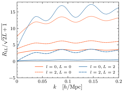
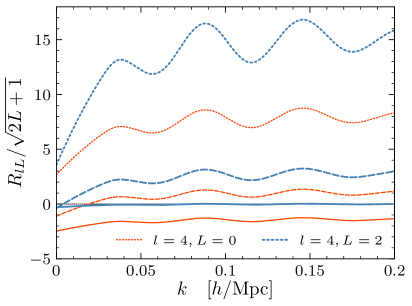
Figure 1: Redshift-space galaxy power spectrum response functions from perturbation theory. The left panel shows the responses only from the physical growth and dilation effects, while the right panel also includes the suppression due to normalization in the power spectrum estimator. The tidal responses are normalized by $\sqrt{5}$ so that the modulating modes $\sqrt{L}\Delta_{L}$ have the same variance for an isotropic window. We use the following values $f=0.757$, $b_{1}=2.2$, $b_{2}=b_{s^{2}}=0$, and a dilation template measured from QPM mock catalogs as detailed in Sec. 3.

In Fig. 1 we show the multipole representation of the response functions, with and without the suppression factors. The suppression changes $R_{00}$ from $\sim 3$ to $\sim-2$ and reverses its sign, meaning for the right combination of $b_{1}$ and $f$ the effect of $R_{00}$ can be minimized. Note that we have divided the tidal responses by $\sqrt{5}$ for comparison with the density responses, given that for an isotropic window the rms mean tide is $1/\sqrt{5}$ times the rms mean overdensity as shown in (2.16).

2.4 Redshift-space dilation

We can rewrite the linear perturbations in the redshift-space galaxy power spectrum $P(k,\mu)$ due to $\Delta_{0}$ and $\Delta_{2}$ as

$$\mathcal{P}^{W}(k,\mu) \simeq\mathcal{P}(k,\mu)\bigl{(}1+G_{0}\Delta_{0}+G_{2}\Delta_{2}\bigr{)}+\frac{\partial\mathcal{P}(k,\mu)}{\partial\ln k}\bigl{(}D_{0}\Delta_{0}+D_{2}\Delta_{2}\bigr{)}$$

$$\simeq\mathcal{P}\bigl{(}k/\alpha(\mu),\mu\bigr{)}+\mathcal{P}(k,\mu)\bigl{(}G_{0}\Delta_{0}+G_{2}\Delta_{2}\bigr{)},$$ (2.38)

where

$$\alpha(\mu)\simeq 1-D_{0}(\mu)\Delta_{0}-D_{2}(\mu)\Delta_{2}$$ (2.39)

is determined by the dilation terms. Obviously this shifts any feature in the power spectrum from its global average $\langle\alpha(\mu)\rangle=1$, which is exactly the reason why the dilation effect is named so. In the above model we have ignored the impact on $\alpha(\mu)$ by the AP effect, which is caused by the distortion due to the assumption of a wrong fiducial cosmology. It is well known that $\Delta_{0}$ induces isotropic dilation of $(1+\Delta_{0})^{\frac{1}{3}}$ in real space, which follows immediately from mass conservation. On top of this, we expect the long-wavelength tidal perturbation and redshift-space distortion would generate anisotropic dilation, and enhance the isotropic one as well.

Taking $\mu=0,1$, we obtain the shift in the transverse and radial directions

$$\delta\alpha_{\perp} \simeq\frac{1}{3}(\Delta_{0}-\Delta_{2}),$$

$$\delta\alpha_{\parallel} \simeq\frac{1}{3}(1+f)(\Delta_{0}+2\Delta_{2}).$$ (2.40)

Therefore the dilation of the volume-averaged distance $\alpha=\alpha_{\parallel}^{\frac{1}{3}}\alpha_{\perp}^{\frac{2}{3}}$ is

$$\delta\alpha\simeq\frac{1}{3}\delta\alpha_{\parallel}+\frac{2}{3}\delta\alpha_{\perp}=\frac{1}{3}\Delta_{0}+\frac{f}{9}(\Delta_{0}+2\Delta_{2}),$$ (2.41)

which one can also derive by averaging $\alpha(\mu)$ over $\mu$ (taking the monopole). If one takes $f\to 0$ and $\Delta_{2}\to 0$, (2.40) and (2.41) fall back to the well known case of real-space isotropic dilation. The anisotropic component is conventionally described by $\epsilon\equiv(\alpha_{\parallel}/\alpha_{\perp})^{\frac{1}{3}}-1$, with

$$\delta\epsilon\simeq\frac{1}{3}\bigl{(}\delta\alpha_{\parallel}-\delta\alpha_{\perp}\bigr{)}=\frac{1}{3}\Delta_{2}+\frac{f}{9}(\Delta_{0}+2\Delta_{2}),$$ (2.42)

which is really half the quadrupole moment of $\alpha(\mu)$. As expected it can arise from either $\Delta_{2}$ or $f$. $\alpha$ and $\epsilon$ constitute an alternative parametrization of $\alpha_{\perp}$ and $\alpha_{\parallel}$ up to quadrupole order.

Importantly, the anisotropic redshift-space dilation breaks the assumption of the AP test that any feature be statistically isotropic provided the fiducial cosmology is the true one. Additionally, the redshift-space dilation also shifts the BAO peak anisotropically. Unlike the shift of the peak due to BAO-scale nonlinear structure formation, this effect is intrinsic to a survey itself and cannot be removed by reconstruction methods without knowing the amplitudes of the long modes beyond scales probed by the survey. We will quantify the impact of super-survey modes on the cosmological constraints from both BAO fitting and full power spectrum shape analysis in Sec. 4.3.

3 Responses in galaxy mock catalogs

Sec. 3.1 describes the galaxy mocks and the estimators to measure response functions from those mocks. In Sec. 3.2 we compare these numerically calibrated responses to the analytic one from Sec. 2.

3.1 QPM mock responses

The quick particle mesh (QPM) [39] method is a fast algorithm to generate galaxy mocks that match abundance and clustering properties. This method selects a subset of PM simulation particles and elevates them as mock dark matter halos based on their local density smoothed on some nonlinear scale. To measure the responses, we exploit $N_{\mathrm{mock}}=991$ QPM mocks of size $2560{\,\mathrm{Mpc}/h}$ originally produced for the BOSS DR12 analysis [40]. We use the mock fiducial values $f=0.757$, $b_{1}=2.2$, and take $b_{2}=b_{s^{2}}=0$ given the QPM algorithm only traces the density.

For each QPM mock we use the galaxy catalog from the full periodic box without the survey mask, and instead sample the short modes by picking galaxies from $N_{\mathrm{sub}}=64$ sub-volumes, each having some nonzero long modes. For robustness we adopt two types of sub-volumes of different geometries and volumes: tiling sub-boxes of size $640{\,\mathrm{Mpc}/h}$, and sub-spheres of radius $320\sqrt{3}{\,\mathrm{Mpc}/h}$ centered on the sub-box vertices. In the following analysis, we always use a $512^{3}$ grid to perform the Fast Fourier Transformation (FFT), and the cubic order scheme to paint galaxies onto the grid [41].

To measure the amplitudes of the long modes, we can simply follow (2.2) and multiply the galaxy field in Fourier space by the sub-volume window and Legendre polynomial, before tranforming backward to read off $b_{1}\Delta_{L}$’s at their corresponding vertex positions in configuration space. By further dividing by $b_{1}$, we can remove the large scale galaxy biasing to obtain the long modes in matter density. Recall that $\Delta_{0}$ and $\Delta_{2}$ are defined in real space, and the latter depends on the LOS direction ${\hat{\mathbf{n}}}$. With so many sub-volumes we can estimate the variance of the long modes $\sigma_{LL}$ accurately.

Next let’s estimate the short-mode power spectrum multipoles $\hat{P}_{l}^{W}$ in redshift space. To improve statistics, for each sub-box we apply RSD by adding peculiar velocities in 6 LOS’s – 3 principle axes and 3 face diagonals, allowing some redundancy given there are only 5 independent components of $\Delta_{2}$. Then we paint the masked full volume onto the FFT grid, before subtracting off the mean using random catalogs (50 times as abundant) inside the sub-volumes and padding with zeros outside. We take advantage of the interlacing technique, which together with the cubic order assignment scheme greatly suppresses aliasing [41]. We then deconvolve the latter [42], subtract the constant shot noise from the squared field, and finally bin the power spectrum multipoles in spherical shells of width $0.01{\,h/\mathrm{Mpc}}$.

Now we can compute the redshift space response functions by correlating $\Delta_{L}$ and $\hat{P}_{l}^{W}$ pairs, with a total of $N_{\mathrm{tot}}=6N_{\mathrm{mock}}N_{\mathrm{sub}}=380544$ realizations,

$$\hat{R}_{lL}(k)=\frac{\sum_{i}^{N_{\mathrm{tot}}}\hat{P}_{li}^{W}\!(k)\,\Delta_{Li}}{N_{\mathrm{tot}}\,P_{l}^{W}(k)\,\sigma_{LL}}=\frac{N_{\mathrm{tot}}\sum_{i}^{N_{\mathrm{tot}}}\hat{P}_{li}^{W}\!(k)\,\Delta_{Li}}{\sum_{i}^{N_{\mathrm{tot}}}\hat{P}_{li}^{W}(k)\sum_{j}^{N_{\mathrm{tot}}}\Delta_{Lj}^{2}}$$ (3.1)

The error is obtained by bootstrapping within all mocks. There are 2 options for the reference number density when measuring $\hat{P}_{l}^{W}$: the average of all mocks or the sub-volume mean. Using the former we will get the response entirely from the physical growth and dilation effect (2.26), while taking the latter we also include the suppression due to local normalization (2.37) To relate to the previous works, the former case is named “global” whereas the latter is referred to as “local” [4].

3.2 Comparison to perturbation theory

Figure 2: Redshift-space response functions from galaxy mocks due to physical growth and dilation effects. Black and grey points with error bars are the mock measurements from sub-boxes and sub-spheres respectively. Lines shows the perturbation theory results.

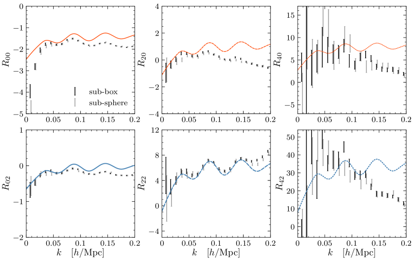
Figure 3: Same as Fig. 2, except that the responses also include suppression resulting from normalization of the estimator. The suppression is about $-5$ for density responses and $-1$ for tidal responses.

Before comparing the analytic predictions in Sec. 2 to the mock response functions, one still needs a dilation template $\operatorname{d}\ln\mathcal{P}/\operatorname{d}\ln k$. We measure this by taking the derivative of the cubic-splined average power spectrum of all the real-space full boxes.

Fig. 2 shows the comparison of mock and analytic redshift-space response functions due to growth and dilation effects, without suppression from the normalization factor of the estimator. The sub-box and sub-sphere results agree with each other throughout the range of $k$, and they are both consistent with the perturbative responses on large scales up to $0.06{\,h/\mathrm{Mpc}}$, beyond which the agreement worsens due to nonlinearity. Here the only exception is that the two mock $R_{00}$’s have some sharp downturn at $k\lesssim 0.03{\,h/\mathrm{Mpc}}$. Given that this scale-dependence is too sharp, and it only occurs in the monopole response to mean density, this feature does not seem to be physical. And indeed the QPM algorithm selects particles to stand in for halos based on the smoothed density, therefore the smoothing scale results in some mode-coupling leading to a large scale scale-dependent bias, which could possibly give rise to such an artifact.

In Fig. 3 we show the same comparison, but in addition to the physical responses we also include the suppression resulting from the normalization factor in the power spectrum estimator as in (2.37). The agreement between the analytic and numerical results is as good as in Fig. 2. Including the suppression from the estimator normalization leads to an offset by about $-5$ for the density responses and approximately $-1$ for the tidal responses. As a result, the density response $R_{00}$ of the power spectrum monopole has its sign reversed, so that its effect could be minimized for the right value of $b_{1}$ and $f$.

4 Super-sample effect

In Sec. 4.1 we briefly review the power spectrum covariance, especially the super-sample covariance due to the presence of long modes, before comparing the SSC model to the one measured from mocks in Sec. 4.2. Finally in Sec. 4.3 we assess the impact of this extra covariance on the BAO, AP, and RSD measurements.

4.1 Redshift space super-sample covariance

Now let’s consider a galaxy survey with size and geometry described by its window function $W$. The statistical precision of power spectrum measurement is described by its covariance. The long modes beyond the size of the survey correlate the observed power spectrum at all wavelengths, giving rise to an additional error known as the super-sample covariance. The covariance of the galaxy power spectrum is defined by

$$C(\mathbf{k}_{1},\mathbf{k}_{2})\equiv\bigl{\langle}\bigl{(}\hat{P}^{W}(\mathbf{k}_{1})-P^{W}(\mathbf{k}_{1})\bigr{)}\bigl{(}\hat{P}^{W}(\mathbf{k}_{2})-P^{W}(\mathbf{k}_{2})\bigr{)}\bigr{\rangle},$$ (4.1)

which can be further decomposed into three pieces based on their statistical and physical origin [3]

$$C(\mathbf{k}_{1},\mathbf{k}_{2})=C^{\mathrm{G}}(\mathbf{k}_{1},\mathbf{k}_{2})+C^{T0}(\mathbf{k}_{1},\mathbf{k}_{2})+C^{\SS}(\mathbf{k}_{1},\mathbf{k}_{2}).$$ (4.2)

The first term is the only nonvanishing piece for a Gaussian random field, and hence its superscript. Therefore we refer the other two terms jointly as the non-Gaussian covariance, in which the second piece arises from direct mode coupling between scales $\mathbf{k}_{1}$ and $\mathbf{k}_{2}$, and the last piece or the super-sample covariance originates from the indirect mode coupling through the coherent modulation by the long modes.

In the small-scale limit ($k_{1},k_{2}\gg V^{-\frac{1}{3}}$) the covariance expressions simplify. The Gaussian covariance becomes diagonal

$$C^{\mathrm{G}}(\mathbf{k}_{1},\mathbf{k}_{2})\simeq\frac{2(2\pi)^{3}}{V_{\mathrm{eff}}}\operatorname{\delta^{\mathrm{D}}}(\mathbf{k}_{1}-\mathbf{k}_{2})\Bigl{(}P(\mathbf{k}_{1})+\frac{1}{\bar{n}}\Bigr{)}^{2},$$ (4.3)

which includes the contribution of a constant shot noise. We have defined an effective volume as

$$V_{\mathrm{eff}}=\frac{V_{2}^{2}}{V_{4}},$$ (4.4)

that differs from that in Ref. [43] in that the former only manifestly includes the volume effect and is not explicitly sensitive to the level of shot noise. And following the notation of Ref. [3] the second term $C^{T0}$, named the trispectrum piece, is given by

$$C^{T0}(\mathbf{k}_{1},\mathbf{k}_{2})\simeq\frac{1}{V_{\mathrm{eff}}}T(\mathbf{k}_{1},-\mathbf{k}_{1},\mathbf{k}_{2},-\mathbf{k}_{2}),$$ (4.5)

where $T$ is the redshift-space galaxy trispectrum or the connected 4-point function

$$\bigl{\langle}\delta(\mathbf{k}_{1})\delta(\mathbf{k}_{2})\delta(\mathbf{k}_{3})\delta(\mathbf{k}_{4})\bigr{\rangle}_{\mathrm{c}}=(2\pi)^{3}\operatorname{\delta^{\mathrm{D}}}\bigl{(}{\textstyle\sum_{i=1}^{4}}\mathbf{k}_{i}\bigr{)}\,T(\mathbf{k}_{1},\mathbf{k}_{2},\mathbf{k}_{3},\mathbf{k}_{4}).$$ (4.6)

Lastly, the super-sample covariance reads intuitively

$$C^{\SS}(\mathbf{k}_{1},\mathbf{k}_{2})=\sum_{L_{1}L_{2}}\sigma_{L_{1}L_{2}}\frac{\operatorname{d}P^{W}(\mathbf{k}_{1})}{\operatorname{d}\Delta_{L_{1}}}\frac{\operatorname{d}P^{W}(\mathbf{k}_{2})}{\operatorname{d}\Delta_{L_{2}}}.$$ (4.7)

In practice one bins the power spectrum in shells of finite width, so that its covariance function reduces to a matrix. Specifically we want to evaluate the Gaussian covariance matrix, which we can subtract from the full covariance matrix to obtain the non-Gaussian piece. Taking the multipole moments in the spherical $\mathbf{k}$-shells labeled by $k_{i},k_{j}$ [44], we get

$$C^{\mathrm{G}}_{l_{1}l_{2}}(k_{i},k_{j})\equiv(2l_{1}+1)(2l_{2}+1)\int_{\begin{subarray}{c}\vspace{1ex}\\ \mathbf{k}_{1}\in V_{k_{i}}\\ \mathbf{k}_{2}\in V_{k_{j}}\end{subarray}}C^{\mathrm{G}}(\mathbf{k}_{1},\mathbf{k}_{2})\operatorname{\mathcal{L}}_{l_{1}}(\mu_{1})\operatorname{\mathcal{L}}_{l_{2}}(\mu_{2})\\ =\frac{2(2l_{1}+1)(2l_{2}+1)\delta_{ij}}{N_{k_{i}}}\sum_{l_{3}l_{4}l_{5}}(2l_{5}+1)\begin{pmatrix}l_{1}&l_{2}&l_{5}\\ 0&0&0\end{pmatrix}^{2}\begin{pmatrix}l_{3}&l_{4}&l_{5}\\ 0&0&0\end{pmatrix}^{2}\int_{\mathbf{k}\in V_{k_{i}}}P_{l_{3}}(k)P_{l_{4}}(k)$$ (4.8)

where the big parentheses are the Wigner 3-j symbols and $N_{k_{i}}\equiv V_{\mathrm{eff}}V_{k_{i}}/(2\pi)^{3}$ is the number of modes in the $i$th shell. The triple sum over $l_{3},l_{4},l_{5}$ runs from 0 to infinity for each $l$, and the summands are nonzero only when the following selection rules are satisfied: $\max(|l_{1}-l_{2}|,|l_{3}-l_{4}|)\leq l_{5}\leq\min(l_{1}+l_{2},l_{3}+l_{4})$, and $l_{5}$ should have the same parity as $l_{1}+l_{2}$ and $l_{3}+l_{4}$ (i.e., even). Note that the shot noise term only shows up with the power spectrum monopoles, and is left implicit here. Similarly the trispectrum piece becomes

$$C_{l_{1}l_{2}}^{T0}(k_{i},k_{j})=\frac{1}{V_{\mathrm{eff}}}T_{l_{1}l_{2}}(k_{i},k_{j}),$$ (4.9)

where

$$T_{l_{1}l_{2}}(k_{i},k_{j})\equiv(2l_{1}+1)(2l_{2}+1)\int_{\begin{subarray}{c}\vspace{1ex}\\ \mathbf{k}_{1}\in V_{k_{i}}\\ \mathbf{k}_{2}\in V_{k_{j}}\end{subarray}}T(\mathbf{k}_{1},-\mathbf{k}_{1},\mathbf{k}_{2},-\mathbf{k}_{2})\operatorname{\mathcal{L}}_{l_{1}}(\mu_{1})\operatorname{\mathcal{L}}_{l_{2}}(\mu_{2}).$$ (4.10)

The super-sample covariance is simply

$$C_{l_{1}l_{2}}^{\SS}(k_{i},k_{j})=P_{l_{1}}(k_{i})P_{l_{2}}(k_{j})\sum_{L_{1}L_{2}}\sigma_{L_{1}L_{2}}R_{l_{1}L_{1}}(k_{i})R_{l_{2}L_{2}}(k_{j}).$$ (4.11)

Eqs. (4.8), (4.9), and (4.11) show clearly how different covariance pieces scale with survey volume and binning. Both $C^{\mathrm{G}}$ and $C^{T0}$ are inversely proportional to $V_{\mathrm{eff}}$ with the former depending in addition on binning, whereas $C^{\SS}$ scales as the covariance of the long modes $\sigma_{L_{1}L_{2}}$. From (2.15), we can see that $\sigma_{L_{1}L_{2}}$ roughly scales as inverse volume when the window size is near the peak of the power spectrum, in which case all three covariance pieces would have the same volume scaling. Increasing the volume beyond that makes $C^{\SS}$ decrease more rapidly than the other two terms. However, this difference in volume scaling is very small, e.g., $V\sigma_{00}(V)$ only decreases by a factor of 2 when a cubic volume $V$ increases from $0.1\,\mathrm{Gpc}^{3}/h^{3}$ to $10\,\mathrm{Gpc}^{3}/h^{3}$ by 2 orders of magnitude.

In the above equations we have omitted the shot noise terms [45] other than the one included in the Gaussian piece. For sufficiently wide bins that have more modes than the number of galaxies $N_{\mathrm{g}}$, those off-diagonal shot noise terms start to become important, with the leading order being $\operatorname{\mathcal{O}}(B/N_{\mathrm{g}})$, where $B$ refers to the bispectrum terms in Eq.8 of Ref. [45]. Higher order terms including $\operatorname{\mathcal{O}}(P/\bar{n}N_{\mathrm{g}})$ and $\operatorname{\mathcal{O}}(1/\bar{n}^{2}N_{\mathrm{g}})$ kick in as well when $\bar{n}P\lesssim 1$.

4.2 Mock covariance

Now let’s examine if the redshift galaxy response functions give rise to the super-sample covariance expected from (4.11), using again the QPM mocks described in Sec. 3.1. If we measure the covariance matrix from the $N_{\mathrm{mock}}$ periodic boxes, the result would only contain the Gaussian and trispectrum contribution since all modes beyond the box size vanish. For each of the 6 LOS, we estimate the covariance matrix among all full boxes

$$\hat{C}_{l_{1}l_{2}}(k_{i},k_{j};{\hat{\mathbf{n}}})=\frac{1}{N_{\mathrm{mock}}-1}\sum_{b=1}^{N_{\mathrm{mock}}}\bigl{(}\hat{P}_{l_{1}b}(k_{i})-P_{l_{1}}(k_{i})\bigr{)}\bigl{(}\hat{P}_{l_{2}b}(k_{j})-P_{l_{2}}(k_{j})\bigr{)}.$$ (4.12)

before averaging over all 6 LOS’s for a combined estimation

$$\hat{C}_{l_{1}l_{2}}(k_{i},k_{j})=\frac{1}{6}\sum_{\hat{\mathbf{n}}}\hat{C}_{l_{1}l_{2}}(k_{i},k_{j};{\hat{\mathbf{n}}}).$$ (4.13)

Given the Gaussian covariance is completely determined by the power spectrum, we can evaluate it using the full box power spectrum multipoles as specified in (4.8). Because $C^{\mathrm{G}}$ is sensitive to the choice of binning, for a clean comparison we would like to subtract it off from (4.13) to obtain the non-Gaussian covariance $\hat{C}^{\textsc{ng}}$ that only depends on survey volume and geometry. In the case of periodic boxes, $\hat{C}^{\textsc{ng}}$ includes the trispectrum piece $C^{T0}_{l_{1}l_{2}}$ and off-diagonal shot noise terms. So it serves as a baseline for comparison with the full covariance matrix including SSC, the latter to be measured from the sub-volumes. Because of the difference in volume between the periodic box and sub-volumes, we need to rescale the periodic covariance by a volume factor of $V/V_{\mathrm{sub}}$ before comparing the two.

The sub-volumes have nonzero long modes above their size, so their covariance contains the SSC piece in $C^{\textsc{ng}}$. To measure it, we can use a estimator similar to the one in (4.12) and (4.13). Because sub-volumes from different mocks are independent, for each LOS and each sub-volume location labeled with $s$, the covariance estimator is

$$\hat{C}_{l_{1}l_{2}}(k_{i},k_{j};{\hat{\mathbf{n}}},s)=\frac{1}{N_{\mathrm{mock}}-1}\sum_{b=1}^{N_{\mathrm{mock}}}\bigl{(}\hat{P}^{W}_{l_{1}b}(k_{i})-P^{W}_{l_{1}}(k_{i})\bigr{)}\bigl{(}\hat{P}^{W}_{l_{2}b}(k_{j})-P^{W}_{l_{2}}(k_{j})\bigr{)}.$$ (4.14)

And then we further average over the LOS’s and sub-volume locations

$$\hat{C}_{l_{1}l_{2}}(k_{i},k_{j})=\frac{1}{6N_{\mathrm{sub}}}\sum_{{\hat{\mathbf{n}}},s}\hat{C}_{l_{1}l_{2}}(k_{i},k_{j};{\hat{\mathbf{n}}},s).$$ (4.15)

We estimate the error on (4.13) and (4.15) by bootstrapping over all $N_{\mathrm{mock}}$ boxes. The masked covariance matrix is affected by the window function and leaks off-diagonally, which can be suppressed in the small-scale wide-bin limit. For simplicity we subtract the volume-scaled diagonal Gaussian covariance (4.8) assuming no window effect. Because of this we expect to underestimate the sub-volume diagonal $C^{\textsc{ng}}$ and slightly overestimate its immediate off-diagonal elements.

To verify our SSC model in (4.11), we can add it to the volume-scaled periodic covariance to see if this reproduces the sub-volume covariance. To evaluate it we use the mean power spectrum multipoles of the periodic boxes, the mock response functions measured in Sec. 3.1, and the covariance of the long modes $\sigma_{L_{1}L_{2}}$ estimated by averaging $\Delta_{L_{1}}\Delta_{L_{2}}$ over all sub-volumes and all LOS’s.

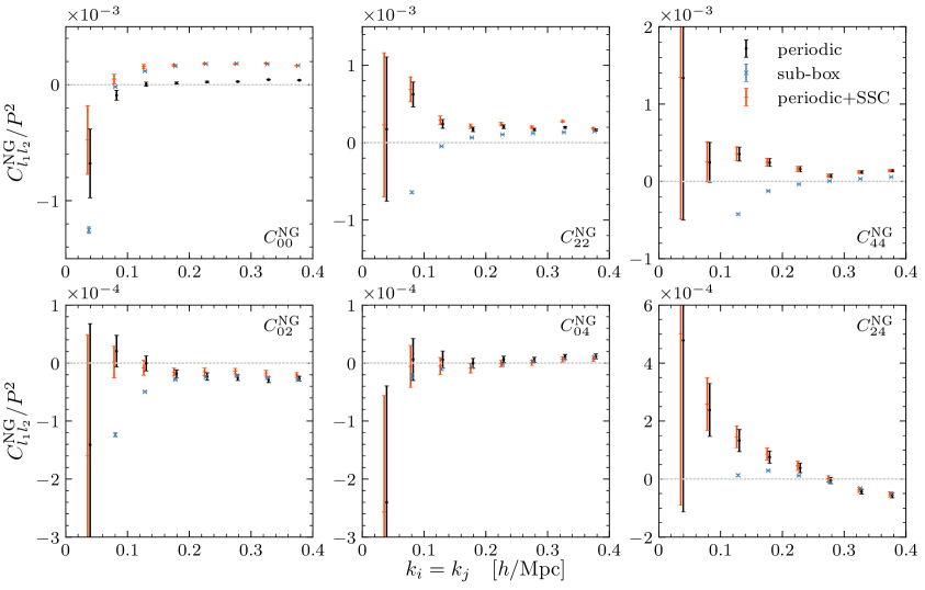
Figure 4: Redshift-space non-Gaussian covariance $C^{\mathrm{NG}}_{l_{1}l_{2}}=\mathrm{cov}(P_{l_{1}}(k_{i}),P_{l_{2}}(k_{j}))$ of galaxy power spectrum multipoles, for diagonal elements $k_{i}=k_{j}$. The covariance is divided by the squared real-space power spectrum.

Fig. 4 shows the non-Gaussian diagonal elements of the auto- and cross-covariance matrices of power spectrum multipoles ($l=0,2,4$) measured from the QPM mocks. We have normalized $C^{\textsc{ng}}$ by the real-space power spectrum $P(k_{i})P(k_{j})$ for a dimensionless quantity. As expected we notice that the sub-box $C^{\textsc{ng}}$ turns negative on large scale due to an over-subtraction of the Gaussian contribution, and more so for larger $l$’s. We have also chosen a wide bin width of $\Delta k=0.05{\,h/\mathrm{Mpc}}$ to suppress the window effect. Clearly the biggest contribution of SSC is to the monopole auto-covariance $C^{\textsc{ng}}_{00}$, in which it dominates over the rest by a factor of $5\sim 10$, where there’s enough statistical precision ($k\gtrsim 0.15{\,h/\mathrm{Mpc}}$). We find that (4.11) models very well the SSC as the difference between periodic and sub-volume covariance. However, SSC does not add significantly to the other $C^{\textsc{ng}}_{l_{1}l_{2}}$’s. This is because not only the SSC becomes smaller for $l>0$, but also the other non-Gaussian terms (trispectrum and shot noise contribution) become much larger. As for the latter cause, the trispectrum term should dominate over the shot noise on large scales where $\bar{n}P\gg 1$. Therefore the fact that $C^{\textsc{ng}}_{22}$ and $C^{\textsc{ng}}_{44}$ are much bigger than the periodic $C^{\textsc{ng}}_{00}$ at $k\approx 0.1{\,h/\mathrm{Mpc}}$ is hinting at some strong angular dependence in the redshift-space galaxy trispectrum (4.5).

Figure 5: Off-diagonal redshift-space non-Gaussian covariance $C^{\mathrm{NG}}_{ll}=\mathrm{cov}(P_{l}(k_{i}),P_{l}(k_{j}))$ of the galaxy power spectrum monopole and quadrupole, evaluated as a function of $k_{i}$ for different fixed $k_{j}$’s marked by vertical lines. The covariance is divided by the squared real-space power spectrum.

In Fig. 5 we show the off-diagonal elements of the auto-covariance matrices of power spectrum multipoles ($l=0,2$) at 3 fixed $k_{j}$’s, binned and normalized in the same way as in Fig. 4. Again because of the leakage due to the window function, the sub-box covariance is underestimated at $k_{i}=k_{j}$ and overestimated in the neighboring bins, especially on the large scale. Similar to Fig. 4, SSC dominates $C^{\textsc{ng}}_{00}$ by a factor of $5\sim 10$ in its off-diagonal elements, but is negligible in all other $C^{\textsc{ng}}_{l_{1}l_{2}}$’s, for which only $C^{\textsc{ng}}_{22}$ is shown here given their qualitative similarity. The three cases of $C^{\textsc{ng}}_{22}$ overlap well with each other, and are about one order of magnitude larger than the periodic $C^{\textsc{ng}}_{00}$. This again implies some interesting angular dependence of the trispectrum term (4.5), which is worth investigating further but is beyond the scope of this paper. Figs. 4 and 5 present the results for the sub-boxes, and we get qualitatively the same results with sub-spheres.

4.3 Impact on BAO, AP, and RSD constraints

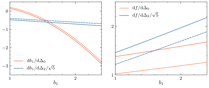
Figure 6: Response of error in $b_{1}$ and $f$ induced by the long modes. We have assumed $f=0.9$(solid), $0.7$(dashed), $b_{2}=0$, $\operatorname{d}\ln\mathcal{P}/\operatorname{d}\ln k\approx 1.5$, $b_{s^{2}}=-4(b_{1}-1)/7$. The tidal responses are normalized by $\sqrt{5}$ so that the modulating modes $\sqrt{L}\Delta_{L}$ have the same variance for an isotropic window.

Because the super-survey modes generate an excess galaxy power spectrum covariance, constraints on cosmological parameters will be degraded due to their stochasticity. In this paper we are interested in the degradation of constraints from spectroscopic galaxy surveys, namely from BAO, AP, and RSD measurements. To evaluate this, a typical approach is the Fisher information analysis (see e.g. [5]). Here we adopt a much simpler and yet equivalently effective approach in three separate steps. We will first demonstrate how to translate the amplitudes of $\Delta_{L}$ to systematic errors on various parameters such as the BAO scale $\alpha$ and growth rate $f$, then show how to assess the size of the effect given the window function using the BOSS survey as an example, and finally compare that to the BOSS DR12 constraint.

The presence of long modes gives rise to systematic errors in BAO and AP straightforwardly according to (2.40), (2.41), and (2.42). The errors on those geometry parameters will further contaminate the conventionally quoted (e.g. [40, 46]) physical quantities, i.e. the angular diameter distance $D_{\mathrm{A}}(z)$, the Hubble expansion rate $H(z)$, the spherically-averaged distance $D_{\mathrm{V}}(z)$, and the AP parameter $F_{\mathrm{AP}}(z)$. The anisotropic BAO measurement constrains $D_{\mathrm{A}}(z)$ and $H(z)$, whose systematic errors translate as

$$\frac{\delta D_{\mathrm{A}}}{D_{\mathrm{A}}}=\delta\alpha_{\perp},\qquad\frac{\delta H}{H}=-\delta\alpha_{\parallel},$$ (4.16)

whereas the isotropic BAO measurement constrains the volume-averaged distance

$$\frac{\delta D_{\mathrm{V}}}{D_{\mathrm{V}}}=\delta\alpha.$$ (4.17)

The AP measurement, for either the BAO scale or the full shape, assumes that any isotropic feature remains isotropic when the fiducial cosmology is exactly the true cosmology. However this assumption is broken by the dilation caused by the long modes, and this can be captured by the following systematic error in the AP parameter

$$\frac{\delta F_{\mathrm{AP}}}{F_{\mathrm{AP}}}=-3\delta\epsilon.$$ (4.18)

To find out how an error on $f$ arises given $\Delta_{0}$ and $\Delta_{2}$, we can fit the perturbed power spectrum multipoles with some $f$ and $b$ offset, which are exactly the systematic error introduced when ignoring the super-sample effect. For simplicity we use our analytic response functions (2.37) and the Kaiser formula (2.24) that are valid on large scale. Assuming that most of the information is from $P_{0}$ and $P_{2}$ and that the responses are approximately scale independent which is true around the relevant scale, one can write down analytically

$$\delta P_{0} =\sum_{L}P_{0}R_{0L}\Delta_{L}=P_{\mathrm{lin}}\bigl{(}2b_{1}\delta b_{1}+\frac{2}{3}b_{1}\delta f+\frac{2}{3}f\delta b_{1}+\frac{2}{5}f\delta f\bigr{)}$$

$$\delta P_{2} =\sum_{L}P_{2}R_{2L}\Delta_{L}=P_{\mathrm{lin}}\bigl{(}\frac{4}{3}b_{1}\delta f+\frac{4}{3}f\delta b_{1}+\frac{8}{7}f\delta f\bigr{)}.$$ (4.19)

By inverting them we derive the linear responses of systematic errors with respect to the long modes $\operatorname{d}b_{1}/\operatorname{d}\Delta_{L}$ and $\operatorname{d}f/\operatorname{d}\Delta_{L}$. In practice the RSD measures the combination $b_{1}\sigma_{8}$ and $f\sigma_{8}$, where $\sigma_{8}$ is the rms density fluctuation in a $8{\,\mathrm{Mpc}/h}$ spherical tophat. For conciseness we do not include the $\sigma_{8}$ factors explicitly in the error response expressions, but this will not affect the result.

Fig. 6 shows these responses as functions of $b_{1}$ and $f$. While we vary $b_{1}$ continuously and choose $f=0.7,0.9$, the other parameters are held fixed $b_{2}=0$, $\operatorname{d}\ln\mathcal{P}/\operatorname{d}\ln k=1.5$, and $b_{s^{2}}=-4(b_{1}-1)/7$. In the left panel, the error response of $b_{1}$ to $\Delta_{2}$ is sensitive to neither $b_{1}$ nor $f$, while its error response to $\Delta_{0}$ is sensitive to $b_{1}$ but not $f$. The former and most of the latter are negative, and at higher bias $b_{1}\gtrsim 1.5$, the latter has a stronger effect. Given that the linear bias is a nuisance parameter, we are mostly interested in the error responses of $f$, which actually does not depend on the value of $b_{2}$. The right panel shows they are more sensitive to $f$ compared to the error responses of $b_{1}$. While the responses to both $\Delta_{0}$ and $\Delta_{2}$ are positive, the effect of the latter is bigger. In most cases, larger $b_{1}$ or $f$ leads to bigger effects.

Table 3: Covariance of super-survey mode for BOSS DR12 NGC for 3 redshift bins, estimated using random catalogs with $N_{\mathrm{r}}=10000$ points.

	$\sqrt{\sigma_{00}}$	$\sqrt{\sigma_{22}}$	$\rho_{02}$
$0.2<z<0.5$	0.0031	0.0015	0.34
$0.4<z<0.6$	0.0029	0.0014	0.39
$0.5<z<0.75$	0.0027	0.0013	0.40

Table 4: Standard deviations of the super-sample errors on various parameters, for the 3 redshift bins of BOSS DR12 NGC. For comparison, the BOSS DR12 constrains $D_{\mathrm{A}}$, $H$, and $f\sigma_{8}$ to $\sim 1.5\%$, $\sim 2\%$, and $\sim 8\%$ precision, respectively, in all redshift bins. Therefore the super-sample errors are of marginal significance for BOSS.

	$\sigma_{D_{\mathrm{A}}}/D_{\mathrm{A}}$	$\sigma_{H}/H$	$\sigma_{D_{\mathrm{V}}}/D_{\mathrm{V}}$	$\sigma_{F_{\mathrm{AP}}}/F_{\mathrm{AP}}$	$\sigma_{b_{1}\sigma_{8}}/b_{1}\sigma_{8}$	$\sigma_{f\sigma_{8}}/f\sigma_{8}$
$0.2<z<0.5$	0.10%	0.29%	0.14%	0.27%	0.4%	1.2%
$0.4<z<0.6$	0.09%	0.27%	0.13%	0.24%	0.3%	1.1%
$0.5<z<0.75$	0.08%	0.26%	0.12%	0.23%	0.3%	1.0%

Given the error responses, we only need the covariance of $\Delta_{L}$’s to estimate the size of super-sample effects. To compute this we apply the random pair summation algorithm presented in App. B to the BOSS DR12 North Galactic Cap (NGC) region using catalogs of $N_{\mathrm{r}}=10000$ random points, for the same three redshift bins as in the BOSS analysis [40], and list the result in Tab. 3. There are two caveats regarding our estimation of $\sigma_{LL^{\prime}}$: we have assumed the plane parallel approximation where all pairs share a common LOS, and have only accounted for the volume of NGC, ignoring the South Galactic Cap (SGC). However, since the NGC sky coverage is limited and NGC is much larger than SGC with about 3 times the number of galaxies, we do not expect drastic difference from a more rigorous treatment. The rms $\Delta_{0}$ is roughly equal to the isotropic value $\sqrt{5}\Delta_{2}$, but slightly larger for lower redshifts. The two super-survey modes are positively correlated, with a significantly nonzero cross-correlation coefficient. This implies that their impacts on the $f\sigma_{8}$ constraint likely add up, given that both $\operatorname{d}f/\operatorname{d}\Delta_{L}$ responses are positive. Similarly, such positive correlation will enhance the super-sample effect on $H(z)$, $D_{\mathrm{V}}(z)$, and $F_{\mathrm{AP}}(z)$, while it partially cancels the impact on $D_{\mathrm{A}}(z)$.

Because $\Delta_{L}$’s are Gaussian modes and the error responses are linear, the systematic errors on various parameters also follows a normal distribution whose variance can be calculated straightforwardly. For all three redshift bins, we combine the effect from the two degrees of freedom and quote the fractional standard deviation $\sigma_{X}/X$ of the systematic error for each parameter $X$ in Tab. 4. To evaluate these, we have taken $f=0.757$, $b_{1}=2.2$ in the responses, and ignored their relatively small evolution with redshift. Comparing these super-sample errors to the BOSS DR12 measurement, we find that the long modes have a much smaller effect $\sim 0.1\%$ than the quoted precision $\sim 1.5\%$ on $D_{\mathrm{A}}(z)$ in all redshift bins. Regarding $H(z)$, the super-survey modes make a relatively bigger impact $\sim 0.3\%$, but is only of marginal significance compared to the BOSS precision $\sim 2\%$. Similarly, the effect on $f\sigma_{8}$ at $\sim 1\%$ is much smaller than the $\sim 8\%$ precision of BOSS measurement.

Future surveys like DESI [47] will put tighter constraint on parameters. While the super-sample effect is likely to remain negligible for the BAO, it can become important for RSD measurements. Comparing to the three BOSS redshift bins [40], the DESI redshift bins between $0.6$ and $1.0$ of width $\delta z=0.1$ have comparable volume and therefore should have similar super-sample error on $f\sigma_{8}$. However, its forecasted error is $2\%\sim 3.3\%$ with $k_{\mathrm{max}}=0.1{\,h/\mathrm{Mpc}}$, and $1\%\sim 1.6\%$ with $k_{\mathrm{max}}=0.2{\,h/\mathrm{Mpc}}$. The super-sample error becomes comparable in size in the latter case, whose forecast seems optimistic for now but promising with recent improvements of nonlinear reconstruction techniques [48, 49, 50] and forward modelling [51]. Therefore we expect the super-sample effect may be non-negligible for RSD measurements from future surveys such as DESI.

5 Conclusion

We consider the impact of long-wavelength modes on the clustering of galaxies in redshift space. It has been well known that the mean density fluctuation in a finite volume will change the local growth and expansion, named the growth effect and the dilation effect respectively. In this paper we have shown that in redshift space both the mean density and tidal modes modulate the local growth and expansion in an angle-dependent way. Out of 5 independent tidal components, only the one along the LOS remains after azimuthal average in redshift space, thus one only needs to consider two long-wavelength modes: the mean density $\Delta_{0}$ and LOS-projection of the mean tide $\Delta_{2}$. We have computed the response of the redshift-space galaxy power spectrum $P(k,\mu)$ to these long modes, at leading order in standard perturbation theory. Our results are in (2.36), (2.3), (2.3), and alternatively when written as responses of multipoles $P_{l}(k)$, in (2.37), Tabs. 1, 2, and Fig. 1. The dilation effect alone coherently shifts all scales according to (2.39), and thus will affect the BAO measurement and the AP effect. This cannot be removed with reconstruction techniques because the effect originates from long modes outside the survey.

In order to verify our analytic results on linear scales, as well as to measure the responses in the quasi-linear regime, we have performed a numerical analysis on about a thousand QPM mocks. Using sub-volumes of two different sizes and shapes, we have estimated both the long modes and the power spectra of those regions. By correlating the two we obtain the nonlinear galaxy response functions. Our numerical (Figs. 2 and 3) and analytic results agree well with each other on large scales, and differ on smaller scales due to the nonlinear RSD.

The galaxy response functions derived in this paper can find applications in the tidal reconstruction method [52, 53] to measure the large-scale tidal field. For optimal extraction of information it is critical to accurately calibrate the response functions into the nonlinear regime using simulations. Separate universe simulations [4, 54, 55, 56, 57, 58, 59, 60, 61, 62, 63, 64, 65] provide an efficient method to measure the response of various observables to the long density mode, such as power spectrum and halo mass function, without sample variance or shot noise. In a similar fashion, the mean tidal mode can be absorbed in the local simulation background at the Newtonian level. We leave this work on tidal simulations and reconstruction for future studies.

The long modes beyond the scale of a survey coherently modulate the galaxy clustering according to their response functions (4.11), leading to an excess power spectrum covariance known as the super-sample covariance. This increased error loosens the constraints on cosmological parameters. Compared to other covariance components, the SSC term scales roughly at the same rate with the volume and thus its effect remains even for much bigger surveys. Because the sub-volume of QPM mocks have non-vanishing long modes, whereas the full periodic volume does not, we have measured the SSC term by comparing their covariance matrices, and confirmed its consistency with the numerical response functions (see Fig. 4 and 5). Interestingly, while the SSC contributes significantly to the monopole $P_{0}$ auto-covariance, it seems negligible in the other covariance blocks, hinting at possible strong angular dependence of the redshift-space galaxy trispectrum.

To assess the impact of the super-sample effect on galaxy clustering, we adopt a simple analytic approach that translates the amplitudes of the long modes to their induced systematic error on observables when ignoring these long modes. To find their typical amplitudes, we have estimated the variance of the super-survey long modes and their correlation (Tab. 3) given the survey window represented by a random catalog. Taking BOSS DR12 as an example, we have found that neglecting the super-sample effect can cause sub-percent to percent levels of systematic error on various parameters constrained by BAO, AP, and RSD measurements, as listed in Tab. 4. Compared to the BOSS DR12 error bars, which are at percent to ten percent levels, this implies that the super-sample effect has only a marginal impact on the constraining power of current spectroscopic galaxy surveys. However our results suggest that for DESI the super-sample error on $f\sigma_{8}$ may become comparable in size to the forecasted error, especially when more small-scale information is made available by iterative reconstruction and forward modelling methods. We therefore expect that the super-sample effect can be non-negligible for RSD measurements in future surveys.

Appendix A Standard perturbation theory

In standard perturbation theory [66], the tree-level matter bispectrum is determined by the $F_{2}$ kernel and the linear matter power spectrum $P_{\mathrm{lin}}$

$$B(\mathbf{k}_{1},\mathbf{k}_{2},\mathbf{k}_{3})=2F_{2}(\mathbf{k}_{1},\mathbf{k}_{2})P_{\mathrm{lin}}(k_{1})P_{\mathrm{lin}}(k_{2})+2\,\mathrm{perm}.$$ (A.1)

The $F_{2}$ kernel is

$$F_{2}(\mathbf{k},\mathbf{k}^{\prime})=\frac{17}{21}+\frac{\mathbf{k}\cdot\mathbf{k}^{\prime}}{2}\Bigl{(}\frac{1}{k^{2}}+\frac{1}{k^{\prime 2}}\Bigr{)}+\frac{4}{21}\operatorname{\mathcal{L}}_{2}({\hat{\mathbf{k}}}\cdot{\hat{\mathbf{k}}}^{\prime}),$$ (A.2)

with the 3 pieces named growth, shift, and tidal terms respectively.

For a galaxy field in redshift space we can introduce the second order biasing and linear RSD effects by using the $Z_{1}$ and $Z_{2}$ kernels [38, 67]. And the tree-level bispectrum of one matter and two galaxy fields is

$$B_{\mathrm{m}\mathrm{g}\mathrm{g}}(\mathbf{k}_{1},\mathbf{k}_{2},\mathbf{k}_{3})=2Z_{2}(\mathbf{k}_{1},\mathbf{k}_{2})Z_{1}(\mathbf{k}_{2})P_{\mathrm{lin}}(k_{1})P_{\mathrm{lin}}(k_{2})+2Z_{2}(\mathbf{k}_{1},\mathbf{k}_{3})Z_{1}(\mathbf{k}_{3})P_{\mathrm{lin}}(k_{1})P_{\mathrm{lin}}(k_{3})\\ +2F_{2}(\mathbf{k}_{2},\mathbf{k}_{3})Z_{1}(\mathbf{k}_{2})Z_{1}(\mathbf{k}_{3})P_{\mathrm{lin}}(k_{2})P_{\mathrm{lin}}(k_{3}).$$ (A.3)

The redshift-space kernels are

$$Z_{1}(\mathbf{k}) =b_{1}+f\frac{(\mathbf{k}\cdot{\hat{\mathbf{n}}})^{2}}{k^{2}}$$ (A.4)

$$Z_{2}(\mathbf{k},\mathbf{k}^{\prime}) =b_{1}F_{2}(\mathbf{k},\mathbf{k}^{\prime})+\frac{b_{1}f(\mathbf{k}+\mathbf{k}^{\prime})\cdot{\hat{\mathbf{n}}}}{2}\Bigl{(}\frac{\mathbf{k}\cdot{\hat{\mathbf{n}}}}{k^{2}}+\frac{\mathbf{k}^{\prime}\cdot{\hat{\mathbf{n}}}}{k^{\prime 2}}\Bigr{)}$$

$$\quad+\frac{f^{2}}{2}\frac{\bigl{[}(\mathbf{k}+\mathbf{k}^{\prime})\cdot{\hat{\mathbf{n}}}\bigr{]}^{2}}{kk^{\prime}}\frac{(\mathbf{k}\cdot{\hat{\mathbf{n}}})(\mathbf{k}^{\prime}\cdot{\hat{\mathbf{n}}})}{kk^{\prime}}+f\frac{\bigl{[}(\mathbf{k}+\mathbf{k}^{\prime})\cdot{\hat{\mathbf{n}}}\bigr{]}^{2}}{(\mathbf{k}+\mathbf{k}^{\prime})^{2}}G_{2}(\mathbf{k},\mathbf{k}^{\prime})$$

$$\quad+\frac{b_{2}}{2}+\frac{b_{s^{2}}}{2}S_{2}(\mathbf{k},\mathbf{k}^{\prime})$$ (A.5)

where ${\hat{\mathbf{n}}}$ is the LOS direction and

$$G_{2}(\mathbf{k},\mathbf{k}^{\prime}) =\frac{13}{21}+\frac{\mathbf{k}\cdot\mathbf{k}^{\prime}}{2}\Bigl{(}\frac{1}{k^{2}}+\frac{1}{k^{\prime 2}}\Bigr{)}+\frac{8}{21}\operatorname{\mathcal{L}}_{2}({\hat{\mathbf{k}}}\cdot{\hat{\mathbf{k}}}^{\prime})$$ (A.6)

$$S_{2}(\mathbf{k},\mathbf{k}^{\prime}) =\Bigl{(}\frac{\mathbf{k}\cdot\mathbf{k}^{\prime}}{kk^{\prime}}\Bigr{)}^{2}-\frac{1}{3}=\frac{2}{3}\operatorname{\mathcal{L}}_{2}({\hat{\mathbf{k}}}\cdot{\hat{\mathbf{k}}}^{\prime})$$ (A.7)

Note that the forms of $F_{2}$ and $G_{2}$ kernels are only exact for flat matter-dominated (Einstein-de Sitter) universe, but are good approximations for cosmologies with $\Omega_{\mathrm{m}}/f^{2}\approx 1$.

To evaluate the real-space squeezed 3-point correlation in (2.10) at tree level, we need to expand the $F_{2}$ kernel of the following forms in $q\ll k$ limit

$$F_{2}(\mathbf{k}+\mathbf{q}_{1},\mathbf{q}_{2})=\frac{17}{21}+\frac{(\mathbf{k}+\mathbf{q}_{1})\cdot\mathbf{q}_{2}}{2q_{2}^{2}}+\frac{4}{21}\operatorname{\mathcal{L}}_{2}({\hat{\mathbf{k}}}\cdot{\hat{\mathbf{q}}}_{2})+\operatorname{\mathcal{O}}(q/k).$$ (A.8)

Because $F_{2}$ starts with $\operatorname{\mathcal{O}}(k/q)$, we should expand the linear power spectrum to $\operatorname{\mathcal{O}}(q/k)$

$$P_{\mathrm{lin}}(\mathbf{k}+\mathbf{q})=(1+\mathbf{q}\cdot\nabla_{\mathbf{k}})P_{\mathrm{lin}}(k)+\operatorname{\mathcal{O}}(q^{2}/k^{2})=\Bigl{(}1+\frac{\mathbf{q}\cdot\mathbf{k}}{k^{2}}\frac{\operatorname{d}\ln P_{\mathrm{lin}}}{\operatorname{d}\ln k}\Bigr{)}P_{\mathrm{lin}}(k)+\operatorname{\mathcal{O}}(q^{2}/k^{2}),$$ (A.9)

so that their combinations expands to $\operatorname{\mathcal{O}}(1)\times P_{\mathrm{lin}}(k)P_{\mathrm{lin}}(q)$, accounting for 2 terms of the 3 permutations in (A.1). The remaining piece takes roughly the form $F_{2}(\mathbf{k},-\mathbf{k}-\mathbf{q})P_{\mathrm{lin}}(k)P_{\mathrm{lin}}(|\mathbf{k}+\mathbf{q}|)$, thus is approximately $\operatorname{\mathcal{O}}(q^{2}/k^{2})\times P_{\mathrm{lin}}^{2}(k)$ when $q\ll k$. Therefore it is much smaller than the other 2 terms given that $P(k)/k^{2}$ is monotonically decreasing, and we’ve dropped it in deriving (2.2).

Similarly for calculation in redshift space, we use the following kernel expansions

$$Z_{1}(\mathbf{k}+\mathbf{q}) =b_{1}+f\frac{(\mathbf{k}\cdot{\hat{\mathbf{n}}})^{2}}{k^{2}}\Bigl{[}1+2\frac{\mathbf{q}\cdot{\hat{\mathbf{n}}}}{\mathbf{k}\cdot{\hat{\mathbf{n}}}}-2\frac{\mathbf{q}\cdot\mathbf{k}}{k^{2}}\Bigr{]}+\operatorname{\mathcal{O}}(q^{2}/k^{2}),$$ (A.10)

$$Z_{2}(\mathbf{k}+\mathbf{q}_{1},\mathbf{q}_{2}) =b_{1}F_{2}(\mathbf{k}+\mathbf{q}_{1},\mathbf{q}_{2})+\frac{b_{1}f}{2}\biggl{\{}\frac{(\mathbf{k}\cdot{\hat{\mathbf{n}}})^{2}}{k^{2}}+\frac{\bigl{[}(\mathbf{k}+\mathbf{q}_{1}+\mathbf{q}_{2})\cdot{\hat{\mathbf{n}}}\bigr{]}(\mathbf{q}_{2}\cdot{\hat{\mathbf{n}}})}{q_{2}^{2}}\biggr{\}}$$

$$\quad+\frac{f^{2}}{2}\frac{(\mathbf{k}\cdot{\hat{\mathbf{n}}})^{3}(\mathbf{q}_{2}\cdot{\hat{\mathbf{n}}})}{k^{2}q_{2}^{2}}\biggl{[}1+\frac{(3\mathbf{q}_{1}+2\mathbf{q}_{2})\cdot{\hat{\mathbf{n}}}}{\mathbf{k}\cdot{\hat{\mathbf{n}}}}-2\frac{\mathbf{q}_{1}\cdot\mathbf{k}}{k^{2}}\biggr{]}$$

$$\quad+f\frac{(\mathbf{k}\cdot{\hat{\mathbf{n}}})^{2}}{k^{2}}G_{2}(\mathbf{k}+\mathbf{q}_{1},\mathbf{q}_{2})+f\frac{(\mathbf{k}\cdot{\hat{\mathbf{n}}})^{2}}{k^{2}}\frac{\mathbf{k}\cdot\mathbf{q}_{2}}{q_{2}^{2}}\biggl{[}\frac{(\mathbf{q}_{1}+\mathbf{q}_{2})\cdot{\hat{\mathbf{n}}}}{\mathbf{k}\cdot{\hat{\mathbf{n}}}}-\frac{(\mathbf{q}_{1}+\mathbf{q}_{2})\cdot\mathbf{k}}{k^{2}}\biggr{]}$$

$$\quad+\frac{b_{2}}{2}+\frac{b_{s^{2}}}{2}S_{2}(\mathbf{k}+\mathbf{q}_{1},\mathbf{q}_{2})+\operatorname{\mathcal{O}}(q/k),$$ (A.11)

where

$$G_{2}(\mathbf{k}+\mathbf{q}_{1},\mathbf{q}_{2}) =\frac{13}{21}+\frac{(\mathbf{k}+\mathbf{q}_{1})\cdot\mathbf{q}_{2}}{2q_{2}^{2}}+\frac{8}{21}\operatorname{\mathcal{L}}_{2}({\hat{\mathbf{k}}}\cdot{\hat{\mathbf{q}}}_{2})+\operatorname{\mathcal{O}}(q/k),$$ (A.12)

$$S_{2}(\mathbf{k}+\mathbf{q}_{1},\mathbf{q}_{2}) =S_{2}(\mathbf{k},\mathbf{q}_{2})+\operatorname{\mathcal{O}}(q/k).$$ (A.13)

The $Z_{1}$ and $P_{\mathrm{lin}}$ factors always occur together in (A.3), so it’s useful to expand this combination using (A.9) and (A.10)

$$Z_{1}(\mathbf{k}+\mathbf{q})P(\mathbf{k}+\mathbf{q})=\biggl{\{}\Bigl{[}b_{1}+f\frac{(\mathbf{k}\cdot{\hat{\mathbf{n}}})^{2}}{k^{2}}\Bigr{]}\Bigl{[}1+\frac{\mathbf{q}\cdot\mathbf{k}}{k^{2}}\frac{\operatorname{d}\ln P}{\operatorname{d}\ln k}\Bigr{]}\\ +2f\frac{(\mathbf{q}\cdot{\hat{\mathbf{n}}})(\mathbf{k}\cdot{\hat{\mathbf{n}}})}{k^{2}}-2f\frac{(\mathbf{k}\cdot{\hat{\mathbf{n}}})^{2}}{k^{2}}\frac{\mathbf{q}\cdot\mathbf{k}}{k^{2}}\biggr{\}}P(k)+\operatorname{\mathcal{O}}(q^{2}/k^{2})$$ (A.14)

Appendix B Estimating covariance of long modes

Figure 7: $\Xi_{L}(r)$ defined in (B.4). We evaluate them with the Python package mcfit that implements the FFTLog algorithm.

Now let’s compute the covariance of $\Delta_{L}$ for $L=0,2$ and some window function $W$, given by (2.15). Spell out each element and expand $\operatorname{\mathcal{L}}_{2}^{2}$ in $\sigma_{22}$ in Legendre series

$$\sigma_{00} =\frac{1}{V_{2}^{2}}\int_{\mathbf{q}}P(q)\bigl{|}\operatorname{\mathcal{W}}(\mathbf{q})\bigr{|}^{2},$$

$$\sigma_{02}=\sigma_{20} =\frac{1}{V_{2}^{2}}\int_{\mathbf{q}}P(q)\bigl{|}\operatorname{\mathcal{W}}(\mathbf{q})\bigr{|}^{2}\operatorname{\mathcal{L}}_{2}({\hat{\mathbf{q}}}\cdot{\hat{\mathbf{n}}}),$$ (B.1)

$$\sigma_{22} =\frac{1}{V_{2}^{2}}\int_{\mathbf{q}}P(q)\bigl{|}\operatorname{\mathcal{W}}(\mathbf{q})\bigr{|}^{2}\Bigl{[}\frac{18}{35}\operatorname{\mathcal{L}}_{4}({\hat{\mathbf{q}}}\cdot{\hat{\mathbf{n}}})+\frac{2}{7}\operatorname{\mathcal{L}}_{2}({\hat{\mathbf{q}}}\cdot{\hat{\mathbf{n}}})+\frac{1}{5}\Bigr{]}.$$

And the Pearson coefficient measures the linear correlation between $\Delta_{0}$ and $\Delta_{2}$

$$\rho_{02}\equiv\frac{\sigma_{02}}{\sqrt{\sigma_{00}\sigma_{22}}}.$$ (B.2)

In order to compute (B.1), one needs to evaluate Fourier space integrals of the following form in (B.3). However this is not easy in Fourier space, as one needs a densely sampled large FFT grid to well resolve and accurately measure $\operatorname{\mathcal{W}}(\mathbf{q})$. So to perform the numerical integration we can rewrite it as a double integral in configuration space

$$\frac{1}{V_{2}^{2}}\int_{\mathbf{q}}P(q)\bigl{|}\operatorname{\mathcal{W}}(\mathbf{q})\bigr{|}^{2}\operatorname{\mathcal{L}}_{L}({\hat{\mathbf{q}}}\cdot{\hat{\mathbf{n}}}) =\frac{1}{V_{2}^{2}}\int\!\frac{q^{2}\operatorname{d}q}{2\pi^{2}}\int_{\hat{\mathbf{q}}}P(q)\operatorname{\mathcal{L}}_{L}({\hat{\mathbf{q}}}\cdot{\hat{\mathbf{n}}})\int_{\mathbf{x}\mathbf{r}}\operatorname{\mathcal{W}}(\mathbf{x})\operatorname{\mathcal{W}}(\mathbf{x}+\mathbf{r})e^{-i\mathbf{q}\cdot\mathbf{r}}$$

$$=\frac{1}{V_{2}^{2}}\int_{\mathbf{x}\mathbf{r}}\Xi_{L}(r)\operatorname{\mathcal{W}}(\mathbf{x})\operatorname{\mathcal{W}}(\mathbf{x}+\mathbf{r})\operatorname{\mathcal{L}}_{L}({\hat{\mathbf{r}}}\cdot{\hat{\mathbf{n}}}),$$ (B.3)

before discretizing it as a double sum. Here we have defined

$$\Xi_{L}(r)\equiv(-i)^{L}\int\!\frac{q^{2}\operatorname{d}q}{2\pi^{2}}\,j_{L}(qr)P(q),$$ (B.4)

where $j_{L}$ is the spherical Bessel function of order $L$. Note that $\Xi_{0}$ is just the correlation function $\xi$, but for higher order $\Xi_{L}$ is different from the correlation function multipoles $\xi_{L}$. $\Xi_{L}(r)$ can be evaluated most efficiently and accurately with the FFTLog algorithm [68]. For this we use the publicly available Python package mcfit and show the result in Fig. 7.

In practice window functions are conveniently approximated by random catalogs of points $\mathbf{x}_{i}$ for $i=1,\cdots,N_{\mathrm{r}}$, whose distribution follows the mean number density of galaxies $\bar{n}(\mathbf{x})$. Thus we can exploit them to discretize the configuration space integrals into sums over random points, by replacing $\int_{\mathbf{x}}\bar{n}\to\frac{N_{\mathrm{g}}}{N_{\mathrm{r}}}\sum_{i=1}^{N_{\mathrm{r}}}$. Recall that $\operatorname{\mathcal{W}}=W^{2}=\bar{n}^{2}w^{2}$. Therefore we can Monte-Carlo the integral (B.3)

$$\frac{1}{V_{2}^{2}}\int_{\mathbf{q}}P(q)\bigl{|}\operatorname{\mathcal{W}}(\mathbf{q})\bigr{|}^{2}\operatorname{\mathcal{L}}_{L}({\hat{\mathbf{q}}}\cdot{\hat{\mathbf{n}}}) \approx\frac{\sum_{i\neq j}\Xi_{L}(r)\bar{n}(\mathbf{x}_{i})\bar{n}(\mathbf{x}_{j})w^{2}(\mathbf{x}_{i})w^{2}(\mathbf{x}_{j})\operatorname{\mathcal{L}}_{L}({\hat{\mathbf{r}}}\cdot{\hat{\mathbf{n}}})}{\bigl{[}\sum_{i}\bar{n}(\mathbf{x}_{i})w^{2}(\mathbf{x}_{i})\bigr{]}^{2}}.$$ (B.5)

where we have removed the shot noise in $|\operatorname{\mathcal{W}}(\mathbf{q})|^{2}$ by omitting the $i=j$ terms in the numerator. To test our method, we populate an $8{\,\mathrm{Mpc}/h}$ tophat with uniform random sample to compute $\sigma_{8}$, and find that only $1000$ random points are needed to reach percent level accuracy.

References

- [1] A. J. S. Hamilton, C. D. Rimes and R. Scoccimarro, On measuring the covariance matrix of the non-linear power spectrum from simulations, MNRAS 371 (Sept., 2006) 1188–1204, [astro-ph/0511416].
- [2] W. Hu and A. V. Kravtsov, Sample Variance Considerations for Cluster Surveys, ApJ 584 (Feb., 2003) 702–715, [astro-ph/0203169].
- [3] M. Takada and W. Hu, Power spectrum super-sample covariance, Phys. Rev. D 87 (June, 2013) 123504, [1302.6994].
- [4] Y. Li, W. Hu and M. Takada, Super-sample covariance in simulations, Phys. Rev. D 89 (Apr., 2014) 083519, [1401.0385].
- [5] Y. Li, W. Hu and M. Takada, Super-sample signal, Phys. Rev. D 90 (Nov., 2014) 103530, [1408.1081].
- [6] C.-T. Chiang, C. Wagner, F. Schmidt and E. Komatsu, Position-dependent power spectrum of the large-scale structure: a novel method to measure the squeezed-limit bispectrum, J. Cosmology Astropart. Phys 5 (May, 2014) 048, [1403.3411].
- [7] C. Wagner, F. Schmidt, C.-T. Chiang and E. Komatsu, The angle-averaged squeezed limit of nonlinear matter N-point functions, J. Cosmology Astropart. Phys 8 (Aug., 2015) 042, [1503.03487].
- [8] F. Schmidt, E. Pajer and M. Zaldarriaga, Large-scale structure and gravitational waves. III. Tidal effects, Phys. Rev. D 89 (Apr., 2014) 083507, [1312.5616].
- [9] K. Akitsu, M. Takada and Y. Li, Large-scale tidal effect on redshift-space power spectrum in a finite-volume survey, Phys. Rev. D 95 (Apr., 2017) 083522, [1611.04723].
- [10] A. Barreira and F. Schmidt, Responses in large-scale structure, J. Cosmology Astropart. Phys 6 (June, 2017) 053, [1703.09212].
- [11] N. Kaiser, Clustering in real space and in redshift space, MNRAS 227 (July, 1987) 1–21.
- [12] A. J. S. Hamilton, Measuring Omega and the real correlation function from the redshift correlation function, ApJ 385 (Jan., 1992) L5–L8.
- [13] M. Feix and A. Nusser, Beyond boundaries of redshift surveys: assessing mass fluctuations on “super-survey“ scales, J. Cosmology Astropart. Phys 12 (Dec., 2013) 027, [1306.4719].
- [14] E. Sefusatti, M. Crocce, S. Pueblas and R. Scoccimarro, Cosmology and the bispectrum, Phys. Rev. D 74 (July, 2006) 023522–+, [arXiv:astro-ph/0604505].
- [15] M. Takada and S. Bridle, Probing dark energy with cluster counts and cosmic shear power spectra: including the full covariance, New Journal of Physics 9 (Dec., 2007) 446, [0705.0163].
- [16] M. Takada and B. Jain, The impact of non-Gaussian errors on weak lensing surveys, MNRAS 395 (June, 2009) 2065–2086, [0810.4170].
- [17] M. Sato, T. Hamana, R. Takahashi, M. Takada, N. Yoshida, T. Matsubara et al., Simulations of Wide-Field Weak Lensing Surveys. I. Basic Statistics and Non-Gaussian Effects, ApJ 701 (Aug., 2009) 945–954, [0906.2237].
- [18] R. Takahashi, N. Yoshida, M. Takada, T. Matsubara, N. Sugiyama, I. Kayo et al., Simulations of Baryon Acoustic Oscillations. II. Covariance Matrix of the Matter Power Spectrum, ApJ 700 (July, 2009) 479–490, [0902.0371].
- [19] M. D. Schneider, S. Cole, C. S. Frenk and I. Szapudi, Fast Generation of Ensembles of Cosmological N-body Simulations Via Mode Resampling, ApJ 737 (Aug., 2011) 11, [1103.2767].
- [20] R. de Putter, C. Wagner, O. Mena, L. Verde and W. J. Percival, Thinking outside the box: effects of modes larger than the survey on matter power spectrum covariance, J. Cosmology Astropart. Phys 4 (Apr., 2012) 019, [1111.6596].
- [21] I. Mohammed and U. Seljak, Analytic model for the matter power spectrum, its covariance matrix and baryonic effects, MNRAS 445 (Dec., 2014) 3382–3400, [1407.0060].
- [22] E. Schaan, M. Takada and D. N. Spergel, Joint likelihood function of cluster counts and n -point correlation functions: Improving their power through including halo sample variance, Phys. Rev. D 90 (Dec., 2014) 123523, [1406.3330].
- [23] I. Mohammed, U. Seljak and Z. Vlah, Perturbative approach to covariance matrix of the matter power spectrum, MNRAS 466 (Apr., 2017) 780–797, [1607.00043].
- [24] C. Howlett and W. J. Percival, Galaxy two-point covariance matrix estimation for next generation surveys, MNRAS 472 (Dec., 2017) 4935–4952, [1709.03057].
- [25] K. C. Chan, A. Moradinezhad Dizgah and J. Noreña, Bispectrum Supersample Covariance, ArXiv e-prints (Sept., 2017) , [1709.02473].
- [26] D. J. Eisenstein, H.-J. Seo, E. Sirko and D. N. Spergel, Improving Cosmological Distance Measurements by Reconstruction of the Baryon Acoustic Peak, ApJ 664 (Aug., 2007) 675–679, [arXiv:astro-ph/0604362].
- [27] V. Marra, L. Amendola, I. Sawicki and W. Valkenburg, Cosmic Variance and the Measurement of the Local Hubble Parameter, Physical Review Letters 110 (June, 2013) 241305, [1303.3121].
- [28] R. Wojtak, A. Knebe, W. A. Watson, I. T. Iliev, S. Heß, D. Rapetti et al., Cosmic variance of the local Hubble flow in large-scale cosmological simulations, MNRAS 438 (Feb., 2014) 1805–1812, [1312.0276].
- [29] I. Ben-Dayan, R. Durrer, G. Marozzi and D. J. Schwarz, Value of H0 in the Inhomogeneous Universe, Physical Review Letters 112 (June, 2014) 221301, [1401.7973].
- [30] K. Ichiki, C.-M. Yoo and M. Oguri, Relationship between the CMB, Sunyaev-Zel’dovich cluster counts, and local Hubble parameter measurements in a simple void model, Phys. Rev. D 93 (Jan., 2016) 023529, [1509.04342].
- [31] I. Odderskov, S. M. Koksbang and S. Hannestad, The local value of H0 in an inhomogeneous universe, J. Cosmology Astropart. Phys 2 (Feb., 2016) 001, [1601.07356].
- [32] H. A. Feldman, N. Kaiser and J. A. Peacock, Power-spectrum analysis of three-dimensional redshift surveys, ApJ 426 (May, 1994) 23–37, [arXiv:astro-ph/9304022].
- [33] N. Kaiser, On the spatial correlations of Abell clusters, ApJ 284 (Sept., 1984) L9–L12.
- [34] J. N. Fry and E. Gaztanaga, Biasing and hierarchical statistics in large-scale structure, ApJ 413 (Aug., 1993) 447–452, [arXiv:astro-ph/9302009].
- [35] P. McDonald and A. Roy, Clustering of dark matter tracers: generalizing bias for the coming era of precision LSS, J. Cosmology Astropart. Phys 8 (Aug., 2009) 020, [0902.0991].
- [36] T. Baldauf, U. Seljak, V. Desjacques and P. McDonald, Evidence for quadratic tidal tensor bias from the halo bispectrum, Phys. Rev. D 86 (Oct., 2012) 083540, [1201.4827].
- [37] K. C. Chan, R. Scoccimarro and R. K. Sheth, Gravity and large-scale nonlocal bias, Phys. Rev. D 85 (Apr., 2012) 083509, [1201.3614].
- [38] R. Scoccimarro, H. M. P. Couchman and J. A. Frieman, The Bispectrum as a Signature of Gravitational Instability in Redshift Space, ApJ 517 (June, 1999) 531–540, [astro-ph/9808305].
- [39] M. White, J. L. Tinker and C. K. McBride, Mock galaxy catalogues using the quick particle mesh method, MNRAS 437 (Jan., 2014) 2594–2606, [1309.5532].
- [40] S. Alam, M. Ata, S. Bailey, F. Beutler, D. Bizyaev, J. A. Blazek et al., The clustering of galaxies in the completed SDSS-III Baryon Oscillation Spectroscopic Survey: cosmological analysis of the DR12 galaxy sample, MNRAS 470 (Sept., 2017) 2617–2652, [1607.03155].
- [41] E. Sefusatti, M. Crocce, R. Scoccimarro and H. M. P. Couchman, Accurate estimators of correlation functions in Fourier space, MNRAS 460 (Aug., 2016) 3624–3636, [1512.07295].
- [42] Y. P. Jing, Correcting for the Alias Effect When Measuring the Power Spectrum Using a Fast Fourier Transform, ApJ 620 (Feb., 2005) 559–563, [astro-ph/0409240].
- [43] M. Tegmark, Measuring Cosmological Parameters with Galaxy Surveys, Physical Review Letters 79 (Nov., 1997) 3806–3809, [astro-ph/9706198].
- [44] J. N. Grieb, A. G. Sánchez, S. Salazar-Albornoz and C. Dalla Vecchia, Gaussian covariance matrices for anisotropic galaxy clustering measurements, MNRAS 457 (Apr., 2016) 1577–1592, [1509.04293].
- [45] A. Meiksin and M. White, The growth of correlations in the matter power spectrum, MNRAS 308 (Oct., 1999) 1179–1184, [astro-ph/9812129].
- [46] F. Beutler, H.-J. Seo, A. J. Ross, P. McDonald, S. Saito, A. S. Bolton et al., The clustering of galaxies in the completed SDSS-III Baryon Oscillation Spectroscopic Survey: baryon acoustic oscillations in the Fourier space, MNRAS 464 (Jan., 2017) 3409–3430, [1607.03149].
- [47] DESI Collaboration, A. Aghamousa, J. Aguilar, S. Ahlen, S. Alam, L. E. Allen et al., The desi experiment part i: Science,targeting, and survey design, ArXiv e-prints (oct, 2016) , [1611.00036].
- [48] H.-M. Zhu, Y. Yu, U.-L. Pen, X. Chen and H.-R. Yu, Nonlinear Reconstruction, ArXiv e-prints (Nov., 2016) , [1611.09638].
- [49] M. Schmittfull, T. Baldauf and M. Zaldarriaga, Iterative initial condition reconstruction, Phys. Rev. D 96 (July, 2017) 023505, [1704.06634].
- [50] Y. Shi, M. Cautun and B. Li, A new method for initial density reconstruction, ArXiv e-prints (Sept., 2017) , [1709.06350].
- [51] U. Seljak, G. Aslanyan, Y. Feng and C. Modi, Towards optimal extraction of cosmological information from nonlinear data, ArXiv e-prints (June, 2017) , [1706.06645].
- [52] U.-L. Pen, R. Sheth, J. Harnois-Deraps, X. Chen and Z. Li, Cosmic Tides, ArXiv e-prints (Feb., 2012) , [1202.5804].
- [53] H.-M. Zhu, U.-L. Pen, Y. Yu, X. Er and X. Chen, Cosmic tidal reconstruction, Phys. Rev. D 93 (May, 2016) 103504, [1511.04680].
- [54] P. McDonald, Toward a Measurement of the Cosmological Geometry at : Predicting Ly Forest Correlation in Three Dimensions and the Potential of Future Data Sets, ApJ 585 (Mar., 2003) 34–51.
- [55] E. Sirko, Initial Conditions to Cosmological N-Body Simulations, or, How to Run an Ensemble of Simulations, ApJ 634 (Nov., 2005) 728–743, [astro-ph/0503106].
- [56] N. Y. Gnedin, A. V. Kravtsov and D. H. Rudd, Implementing the DC Mode in Cosmological Simulations with Supercomoving Variables, ApJS 194 (June, 2011) 46, [1104.1428].
- [57] T. Baldauf, U. Seljak, L. Senatore and M. Zaldarriaga, Galaxy bias and non-linear structure formation in general relativity, J. Cosmology Astropart. Phys 10 (Oct., 2011) 31, [1106.5507].
- [58] C. Wagner, F. Schmidt, C.-T. Chiang and E. Komatsu, Separate universe simulations, MNRAS 448 (Mar., 2015) L11–L15, [1409.6294].
- [59] Y. Li, W. Hu and M. Takada, Separate universe consistency relation and calibration of halo bias, Phys. Rev. D 93 (Mar., 2016) 063507, [1511.01454].
- [60] T. Lazeyras, C. Wagner, T. Baldauf and F. Schmidt, Precision measurement of the local bias of dark matter halos, J. Cosmology Astropart. Phys 2 (Feb., 2016) 018, [1511.01096].
- [61] T. Baldauf, U. Seljak, L. Senatore and M. Zaldarriaga, Linear response to long wavelength fluctuations using curvature simulations, J. Cosmology Astropart. Phys 9 (Sept., 2016) 007, [1511.01465].
- [62] W. Hu, C.-T. Chiang, Y. Li and M. LoVerde, Separating the Universe into real and fake energy densities, Phys. Rev. D 94 (July, 2016) 023002, [1605.01412].
- [63] C.-T. Chiang, Y. Li, W. Hu and M. LoVerde, Quintessential scale dependence from separate universe simulations, Phys. Rev. D 94 (Dec., 2016) 123502, [1609.01701].
- [64] C.-T. Chiang, W. Hu, Y. Li and M. LoVerde, Scale-dependent bias and bispectrum in neutrino separate universe simulations, ArXiv e-prints (Oct., 2017) , [1710.01310].
- [65] A. M. Cieplak and A. Slosar, Towards physics responsible for large-scale Lyman- forest bias parameters, J. Cosmology Astropart. Phys 3 (Mar., 2016) 016, [1509.07875].
- [66] F. Bernardeau, S. Colombi, E. Gaztanaga and R. Scoccimarro, Large-scale structure of the Universe and cosmological perturbation theory., Phys. Rep. 367 (2002) 1–128.
- [67] H. Gil-Marín, C. Wagner, J. Noreña, L. Verde and W. Percival, Dark matter and halo bispectrum in redshift space: theory and applications, J. Cosmology Astropart. Phys 12 (Dec., 2014) 029, [1407.1836].
- [68] A. J. S. Hamilton, Uncorrelated modes of the non-linear power spectrum, MNRAS 312 (Feb., 2000) 257–284, [astro-ph/9905191].