Getting acquainted with the fractional Laplacian

Abstract.

These are the handouts of an undergraduate minicourse at the Università di Bari (see Figure 1), in the context of the 2017 INdAM Intensive Period “Contemporary Research in elliptic PDEs and related topics”. Without any intention to serve as a throughout epitome to the subject, we hope that these notes can be of some help for a very initial introduction to a fascinating field of classical and modern research.

1. The Laplace operator

The operator mostly studied in partial differential equations is likely the so-called Laplacian, given by

(1.1) $$-\Delta u(x):=-\sum_{j=1}^{n}\frac{\partial^{2}u}{\partial x_{j}^{2}}(x)=\lim_{r\searrow 0}\frac{\,{\rm const}\,}{r^{n+2}}\,\int_{B_{r}(x)}\big{(}u(x)-u(y)\big{)}\,dy{=-\,{\rm const}\,\int_{\partial B_{1}}D^{2}u(x)\,\theta\cdot\theta\,d\theta}$$

Of course, one may wonder why mathematicians have a strong preference for such kind of operators – say, why not studying

$$\frac{\partial^{7}u}{\partial x_{1}^{7}}(x)-\frac{\partial^{8}u}{\partial x_{2}^{8}}(x)+\frac{\partial^{9}u}{\partial x_{3}^{9}}(x)-\frac{\partial^{10}u}{\partial x_{1}\partial x_{2}^{4}\partial x_{3}^{5}}(x)\quad\;?$$

Since historical traditions, scientific legacies or impositions from above by education systems would not be enough to justify such a strong interest in only one operator (plus all its modifications), it may be worth to point out a simple geometric property enjoyed by the Laplacian (and not by many other operators). Namely, equation (1.1) somehow reveals that the fact that a function is harmonic (i.e., that its Laplace operator vanishes in some region) is deeply related to the action of “comparing with the surrounding values and reverting to the averaged values in the neighborhood”.

Figure 1. Working hard (and profitably) in Bari.

To wit, the idea behind the integral representation of the Laplacian in formula (1.1) is that the Laplacian tries to model an “elastic” reaction: the vanishing of such operator should try to “revert the value of a function at some point to the values nearby”, or, in other words, from a “political” perspective, the Laplacian is a very “democratic” operator, which aims at levelling out differences in order to make things as uniform as possible. In mathematical terms, one looks at the difference between the values of a given function $u$ and its average in a small ball of radius $r$, namely

$$\textswab{d}_{r}(x):=u(x)\,-\,\mathchoice{{\vbox{\hbox{$\textstyle\overline{\quad}$ }}\kern-7.50009pt}}{{\vbox{\hbox{$\scriptstyle\overline{\quad}$ }}\kern-7.50009pt}}{{\vbox{\hbox{$\scriptscriptstyle\overline{\quad}$ }}\kern-6.75008pt}}{{\vbox{\hbox{$\scriptscriptstyle\overline{\quad}$ }}\kern-6.25006pt}}\!\int_{B_{r}(x)}u(y)\,dy=\mathchoice{{\vbox{\hbox{$\textstyle\overline{\quad}$ }}\kern-7.50009pt}}{{\vbox{\hbox{$\scriptstyle\overline{\quad}$ }}\kern-7.50009pt}}{{\vbox{\hbox{$\scriptscriptstyle\overline{\quad}$ }}\kern-6.75008pt}}{{\vbox{\hbox{$\scriptscriptstyle\overline{\quad}$ }}\kern-6.25006pt}}\!\int_{B_{r}(x)}\big{(}u(x)-u(y)\big{)}\,dy.$$

In the smooth setting, a second order Taylor expansion of $u$ and a cancellation in the integral due to odd symmetry show that $\textswab{d}_{r}$ is quadratic in $r$, hence, in order to detect the “elastic”, or “democratic”, effect of the model at small scale, one has to divide by $r^{2}$ and take the limit as $r\searrow 0$. This is exactly the procedure that we followed in formula (1.1).

Other classical approaches to integral representations of elliptic operators come in view of potential theory and inversion operators, see e.g. [MR0030102].

This tendency to revert to the surrounding mean suggests that harmonic equations, or in general equations driven by operators “similar to the Laplacian”, possess some kind of rigidity or regularity properties that prevents the solutions to oscillate too much (of course, detecting and establishing these properties is a marvelous, and technically extremely demanding, success of modern mathematics, and we do not indulge in this set of notes on this topic of great beauty and outmost importance, and we refer, e.g. to the classical books [MR1625845, MR1814364, MR1962933, MR2777537]).

Interestingly, the Laplacian operator, in the perspective of (1.1), is the infinitesimal limit of integral operators. In the forthcoming sections, we will discuss some other integral operators, which recover the Laplacian in an appropriate limit, and which share the same property of averaging the values of the function. Differently from what happens in (1.1), such averaging procedure will not be necessarily confined to a small neighborhood of a given point, but will rather tend to comprise all the possible values of a certain function, by possibly “weighting more” the close-by points and “less” the contributions coming from far.

2. Some fractional operators

We describe here the basics of some different fractional operators. The fractional exponent will be denoted by $s\in(0,1)$. For more exhaustive discussions and comparisons see e.g. [MR0290095, MR0350027, MR1347689, MR2676137, MR2944369, MR3233760, MR3246044, MR3469920, MR3613319]. For simplicity, we do not treat here the case of fractional operators of order higher than $1$ (see e.g. [GD, AJS1, AJS2, AJS3]).

2.1. The fractional Laplacian

A very popular nonlocal operator is given by the fractional Laplacian

(2.1) $$(-\Delta)^{s}u(x):=\,{\rm P.V.}\,\int_{\mathbb{R}^{n}}\frac{u(x)-u(y)}{|x-y|^{n+2s}}\,dy.$$

Here above, the notation “$\,{\rm P.V.}\,$” stands for “in the Principal Value sense”, that is

$$(-\Delta)^{s}u(x):=\lim_{\varepsilon\searrow 0}\int_{\mathbb{R}^{n}\setminus B_{\varepsilon}(x)}\frac{u(x)-u(y)}{|x-y|^{n+2s}}\,dy.$$

The definition in (2.1) differs from others available in the literature since a normalizing factor has been omitted for the sake of simplicity: this multiplicative constant is only important in the limits as $s\nearrow 1$ and $s\searrow 0$, but plays no essential role for a fixed fractional parameter $s\in(0,1)$.

The operator in (2.1) can be also conveniently written in the form

(2.2) $$-(-\Delta)^{s}u(x)=\frac{1}{2}\int_{\mathbb{R}^{n}}\frac{u(x+y)+u(x-y)-2u(x)}{|y|^{n+2s}}\,dy.$$

The expression in (2.2) reveals that the fractional Laplacian is a sort of second order difference operator, weighted by a measure supported in the whole of $\mathbb{R}^{n}$ and with a polynomial decay, namely

(2.3) $$\begin{split}&-(-\Delta)^{s}u(x)=\frac{1}{2}\int_{\mathbb{R}^{n}}\delta_{u}(x,y)\,d\mu(y),\\ {\mbox{ where }}\quad&\delta_{u}(x,y):=u(x+y)+u(x-y)-2u(x)\quad{\mbox{ and }}\quad d\mu(y):=\frac{dy}{|y|^{n+2s}}.\end{split}$$

Of course, one can give a pointwise meaning of (2.1) and (2.2) if $u$ is sufficiently smooth and with a controlled growth at infinity (and, in fact, it is possible to set up a suitable notion of fractional Laplacian also for functions that grow polynomially at infinity, see [POLYN]). Besides, it is possible to provide a functional framework to define such operator in the weak sense (see e.g. [MR2879266]) and a viscosity solution approach is often extremely appropriate to construct general regularity theories (see e.g. [MR2494809]).

We refer to [MR2944369] for a gentle introduction to the fractional Laplacian.

From the point of view of the Fourier Transform, denoted, as usual, by $\widehat{\cdot}$ or by ${\mathcal{F}}$ (depending on the typographical convenience), an instructive computation (see e.g. Proposition 3.3 in [MR2944369]) shows that

$$\widehat{(-\Delta)^{s}u}(\xi)=c\,|\xi|^{2s}\,\widehat{u}(\xi),$$

for some $c>0$. An appropriate choice of the normalization constant in (2.1) (also in dependence of $n$ and $s$) allows us to take $c=1$, and we will take this normalization for the sake of simplicity (and with the slight abuse of notation of dropping constants here and there). With this choice, the fractional Laplacian in Fourier space is simply the multiplication by the symbol $|\xi|^{2s}$, consistently with the fact that the classical Laplacian corresponds to the multiplication by $|\xi|^{2}$. In particular, the fractional Laplacian recovers the classical Laplacian as $s\nearrow 1$. In addition, it satisfies the semigroup property, for any $s$, $s^{\prime}\in(0,1)$ with $s+s^{\prime}\leqslant 1$,

$${\mathcal{F}}{(-\Delta)^{s}(-\Delta)^{s^{\prime}}u}=|\xi|^{2s}\,{\mathcal{F}}((-\Delta)^{s^{\prime}}u)=|\xi|^{2s}\,|\xi|^{2s^{\prime}}\,\widehat{u}=|\xi|^{2(s+s^{\prime})}\,\widehat{u}={\mathcal{F}}{(-\Delta)^{s+s^{\prime}}u},$$

that is

(2.4) $$(-\Delta)^{s}(-\Delta)^{s^{\prime}}u=(-\Delta)^{s^{\prime}}(-\Delta)^{s}u=(-\Delta)^{s+s^{\prime}}u.$$

As a special case of (2.4), when $s=s^{\prime}=1/2$, we have that the square root of the Laplacian applied twice produces the classical Laplacian, namely

(2.5) $$\Big{(}(-\Delta)^{1/2}\Big{)}^{2}=-\Delta.$$

This observation gives that if $U:\mathbb{R}^{n}\times[0,+\infty)\to\mathbb{R}$ is the harmonic extension of $u:\mathbb{R}^{n}\to\mathbb{R}$, i.e. if

(2.6) $$\left\{\begin{matrix}\Delta U=0&{\mbox{ in }}\mathbb{R}^{n}\times[0,+\infty),\\ U(x,0)=u(x)&{\mbox{ for any }}x\in\mathbb{R}^{n},\end{matrix}\right.$$

then

(2.7) $$-\partial_{y}U(x,0)=(-\Delta)^{1/2}u(x).$$

See Appendix A for a confirmation of this. In a sense, formula (2.7) is a particular case of a general approach which reduces the fractional Laplacian to a local operator which is set in a halfspace with an additional dimension and may be of singular or degenerate type, see [MR2354493].

As a rather approximative “general nonsense”, we may say that the fractional Laplacian shares some common feature with the classical Laplacian. In particular, both the classical and the fractional Laplacian are invariant under translations and rotations. Moreover, a control on the size of the fractional Laplacian of a function translates, in view of (2.3), into a control of the oscillation of the function (though in a rather “global” fashion): this “democratic” tendency of the operator of “averaging out” any unevenness in the values of a function is indeed typical of “elliptic” operators – and the classical Laplacian is the prototype example in this class of operators, while the fractional Laplacian is perhaps the most natural fractional counterpart.

To make this counterpart more clear, we will say that a function $u$ is $s$-harmonic in a set $\Omega$ if $(-\Delta)^{s}u=0$ at any point of $\Omega$ (for simplicity, we take this notion in the “strong” sense, but equivalently one could look at distributional definitions, see e.g. Theorem 3.12 in [MR1671973]).

For example, constant functions in $\mathbb{R}^{n}$ are $s$-harmonic in the whole space for any $s\in(0,1)$, as both (2.1) and (2.2) imply.

Another similarity between classical and fractional Laplace equations is given by the fact that notions like those of fundamental solutions, Green functions and Poisson kernels are also well-posed in the fractional case and somehow similar formulas hold true, see e.g. Definitions 1.7 and 1.8, and Theorems 2.3, 2.10, 3.1 and 3.2 in [MR3461641] (and related formulas hold true also for higher-order fractional operators, see [GD, AJS1, AJS2, AJS3]).

In addition, space inversions such as the Kelvin Transform also possess invariant properties in the fractional framework, see e.g. [MR2256481] (see also Lemma 2.2 and Corollary 2.3 in [MR2964681], and in addition Proposition A.1 on page 300 in [MR3168912] for a short proof). Moreover, fractional Liouville-type results hold under various assumptions, see e.g. [MR3511811] and [POLYN].

Another interesting link between classical and fractional operators is given by subordination formulas which permit to reconstruct fractional operators from the heat flow of classical operators, such as

$$(-\Delta)^{s}u=-\frac{s}{\Gamma(1-s)}\int_{0}^{+\infty}t^{-1-s}\Big{(}e^{t\Delta}-1\Big{)}u\,dt,$$

see [MR0115096].

In spite of all these similarities, many important structural differences between the classical and the fractional Laplacian arise. Let us list some of them.

Difference 2.1 (Locality versus nonlocality).

The classical Laplacian of $u$ at a point $x$ only depends on the values of $u$ in $B_{r}(x)$, for any $r>0$.

This is not true for the fractional Laplacian. For instance, if $u\in C^{\infty}_{0}(B_{2},\,[0,1])$ with $u=1$ in $B_{1}$, we have that, for any $x\in\mathbb{R}^{n}\setminus B_{4}$,

(2.8) $$-(-\Delta)^{s}u(x)=\,{\rm P.V.}\,\int_{\mathbb{R}^{n}}\frac{u(y)-u(x)}{|x-y|^{n+2s}}\,dy=\int_{B_{2}}\frac{u(y)}{|x-y|^{n+2s}}\,dy\geqslant\int_{B_{1}}\frac{dy}{\big{(}|x|+1\big{)}^{n+2s}}\geqslant\frac{\,{\rm const}\,}{|x|^{n+2s}}$$

while of course $\Delta u(x)=0$ in this setting.

It is worth remarking that the estimate in (2.8) is somewhat optimal. Indeed, if $u$ belongs to the Schwartz space (or space of rapidly decreasing functions)

(2.9) $${\mathcal{S}}:=\left\{u\in C^{\infty}(\mathbb{R}^{n}){\mbox{ s.t. }}\sup_{x\in\mathbb{R}^{n}}|x|^{\alpha}\left|D^{\beta}u(x)\right|<+\infty{\mbox{ for all }}\alpha,\beta\in\mathbb{N}^{n}\right\},$$

we have that, for large $|x|$,

(2.10) $$\big{|}(-\Delta)^{s}u(x)\big{|}\leqslant\frac{\,{\rm const}\,}{|x|^{n+2s}}.$$

See Appendix B for the proof of this fact.

Difference 2.2 (Summability assumptions).

The pointwise computation of the classical Laplacian on a function $u$ does not require integrability properties on $u$. Conversely, formula (2.1) for $u$ can make sense only when

$$\int_{\mathbb{R}^{n}}\frac{|u(y)|}{1+{|y|}^{n+2s}}\;dy\ <\ +\infty$$

which can be read as a local integrability complemented by a growth condition at infinity. This feature, which could look harmless at a first glance, can result problematic when looking for singular solutions to nonlinear problems (as, for example, in [MR2985500, MR3393247] where there is an unavoidable integrability obstruction on a bounded domain) or in “blow-up” type arguments (as mentioned in [POLYN], where the authors propose a way to outflank this restriction).

Difference 2.3 (Computation along coordinate directions).

The classical Laplacian of $u$ at the origin only depends on the values that $u$ attains along the coordinate directions (or, up to a rotation, along a set of $n$ orthogonal directions).

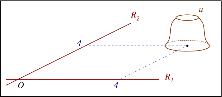
Figure 2. Coordinate directions not meeting a bump function.

This is not true for the fractional Laplacian. As an example, let $u\in C^{\infty}_{0}(B_{2}(4e_{1}+4e_{2}),\,[0,1])$, with $u=1$ in $B_{1}(4e_{1}+4e_{2})$. Let also $R_{j}$ be the straight line in the $j$th coordinate direction, that is

$$R_{j}:=\{te_{j},\;t\in\mathbb{R}\},$$

see Figure 2. Then

$$R_{j}\cap B_{2}(4e_{1}+4e_{2})=\varnothing$$

for each $j\in\{1,\dots,n\}$, and so $u(te_{j})=0$ for all $t\in\mathbb{R}$ and $j\in\{1,\dots,n\}$. This gives that $\Delta u(0)=0$.

On the other hand,

$$\int_{\mathbb{R}^{n}}\frac{u(y)-u(0)}{|0-y|^{n+2s}}\,dy=\int_{\mathbb{R}^{n}}\frac{u(y)}{|y|^{n+2s}}\,dy\geqslant\int_{B_{1}(4e_{1}+4e_{2})}\frac{dy}{|y|^{n+2s}}>0,$$

which says that $(-\Delta)^{s}u(0)\neq 0$.

Difference 2.4 (Harmonic versus $s$-harmonic functions).

If $\Delta u(0)=1$, $\|u-v\|_{C^{2}(B_{1})}\leqslant\varepsilon$ and $\varepsilon>0$ is sufficiently small (see Figure 3) then $\Delta v(0)\geqslant 1-\,{\rm const}\,\varepsilon>0$, and in particular $\Delta v(0)\neq 0$.

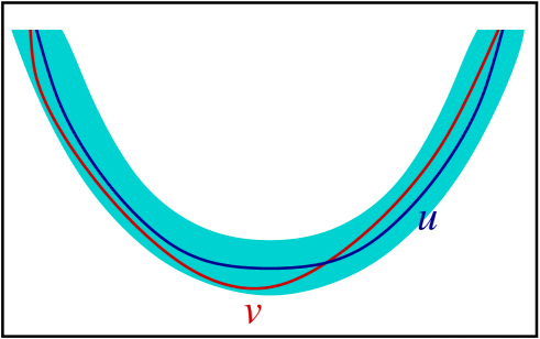
Figure 3. A function $v$ which is “close to $u$”.

Quite surprisingly, this is not true for the fractional Laplacian. More generally, in this case, as proved in [MR3626547], for any $\varepsilon>0$ and any (bounded, smooth) function $\bar{u}$, we can find $v_{\varepsilon}$ such that

(2.11) $$\left\{\begin{matrix}\|\bar{u}-v_{\varepsilon}\|_{C^{2}(B_{1})}\leqslant\varepsilon\\ {\mbox{and }}(-\Delta)^{s}v_{\varepsilon}=0{\mbox{ in }}B_{1}.\end{matrix}\right.$$

A proof of this fact in dimension $1$ for the sake of simplicity is given in [HB] (the original paper [MR3626547] presents a complete proof in any dimension). See also [SALO1, SALO2, SALO3] for different approaches to approximation methods in fractional settings which lead to new proofs, and very refined and quantitative statements.

We also mention that the phenomenon described in (2.11) (which can be summarized in the evocative statement that all functions are locally $s$-harmonic (up to a small error)) is very general, and it applies to other nonlocal operators, also independently from their possibly “elliptic” structure (for instance all functions are locally $s$-caloric, or $s$-hyperbolic, etc.). In this spirit, for completeness, in Section 5 we will establish the density of fractional caloric functions in one space variable, namely of the fact that for any $\varepsilon>0$ and any (bounded, smooth) function $\bar{u}=\bar{u}(x,t)$, we can find $v_{\varepsilon}=v_{\varepsilon}(x,t)$ such that

(2.12) $$\left\{\begin{matrix}\|\bar{u}-v_{\varepsilon}\|_{C^{2}((-1,1)\times(-1,1))}\leqslant\varepsilon\\ {\mbox{and }}\partial_{t}v_{\varepsilon}+(-\Delta)^{s}v_{\varepsilon}=0{\mbox{ for any }}x\in(-1,1){\mbox{ and any }}t\in(-1,1).\end{matrix}\right.$$

We also refer to [SCALOR] for a general approach and a series of general results on this type of approximation problems with solutions of operators which are the superposition of classical differential operators with fractional Laplacians. Furthermore, similar results hold true for other nonlocal operators with memory, see [ESAIM]. See in addition [2018arXiv180904005C, 2018arXiv181007648K, 2018arXiv181008448C] for related results on higher order fractional operators.

Difference 2.5 (Harnack Inequality).

The classical Harnack Inequality says that if $u$ is harmonic in $B_{1}$ and $u\geqslant 0$ in $B_{1}$ then

$$\inf_{B_{1/2}}u\geqslant\,{\rm const}\,\sup_{B_{1/2}}u,$$

for a suitable universal constant, only depending on the dimension.

The same result is not true for $s$-harmonic functions. To construct an easy counterexample, let $\bar{u}(x)=|x|^{2}$ and, for a small $\varepsilon>0$, let $v_{\varepsilon}$ be as in (2.11). Notice that, if $x\in B_{1}\setminus B_{1/4}$

(2.13) $$v_{\varepsilon}(x)\geqslant\bar{u}(x)-\|\bar{u}-v_{\varepsilon}\|_{L^{\infty}(B_{1})}\geqslant\frac{1}{16}-\varepsilon>\frac{1}{32}$$

if $\varepsilon$ is small enough, while

$$v_{\varepsilon}(0)\leqslant\bar{u}(0)+\|\bar{u}-v_{\varepsilon}\|_{L^{\infty}(B_{1})}\leqslant 0+\varepsilon<\frac{1}{32}.$$

These observations imply that $v_{\varepsilon}(0)<v_{\varepsilon}(x)$ for all $x\in B_{1}\setminus B_{1/4}$ and therefore the infimum of $v_{\varepsilon}$ in $B_{1}$ is taken at some point $\bar{x}$ in the closure of $B_{1/4}$. Then, we define

$$u_{\varepsilon}(x):=v_{\varepsilon}(x)-\inf_{{B_{1}}}v_{\varepsilon}=v_{\varepsilon}(x)-v_{\varepsilon}(\bar{x}).$$

Notice that $u_{\varepsilon}$ is $s$-harmonic in $B_{1}$, since so is $v_{\varepsilon}$, and $u_{\varepsilon}\geqslant 0$ in $B_{1}$. Also, $u_{\varepsilon}$ is strictly positive in $B_{1}\setminus B_{1/4}$. On the other hand, since $\bar{x}\in B_{1/2}$

$$\inf_{B_{1/2}}u_{\varepsilon}=u_{\varepsilon}(\bar{x})=0,$$

which implies that $u_{\varepsilon}$ cannot satisfy a Harnack Inequality as the one in (2.13).

In any case, it must be said that suitable Harnack Inequalities are valid also in the fractional case, under suitable “global” assumptions on the solution: for instance, the Harnack Inequality holds true for solutions that are positive in the whole of $\mathbb{R}^{n}$ rather than in a given ball. We refer to [MR1941020, MR2817382] for a comprehensive discussion on this topic and for recent developments.

Difference 2.6 (Growth from the boundary).

Roughly speaking, solutions of Laplace equations have “linear (i.e. Lipschitz) growth from the boundary”, while solutions of fractional Laplace equations have only Hölder growth from the boundary. To understand this phenomenon, we point out that if $u$ is continuous in the closure of $B_{1}$, with $\Delta u=f$ in $B_{1}$ and $u=0$ on $\partial B_{1}$, then

(2.14) $$|u(x)|\leqslant\,{\rm const}\,(1-|x|)\,\sup_{B_{1}}|f|.$$

Notice that the term $(1-|x|)$ represents the distance of the point $x\in B_{1}$ from $\partial B_{1}$. See e.g. Appendix C for a proof of (2.14).

The case of fractional equations is very different. A first example which may be useful to keep in mind is that the function

(2.15) $$\begin{split}&\mathbb{R}^{n}\ni x\mapsto(x_{n})_{+}^{s}\\ &{\mbox{is $s$-harmonic in the halfspace\leavevmode\nobreak\ $\{x_{n}>0\}$.}}\end{split}$$

For an elementary proof of this fact, see e.g. Section 2.4 in [MR3469920]. Remarkably, the function in (2.15) is only Hölder continuous with Hölder exponent $s$ near the origin.

Another interesting example is given by the function

(2.16) $$\mathbb{R}\ni x\mapsto u_{1/2}(x):=(1-|x|^{2})_{+}^{1/2},$$

which satisfies

(2.17) $$(-\Delta)^{1/2}\,u_{1/2}=\,{\rm const}\,\quad{\mbox{ in }}\;(-1,1).$$

A proof of (2.17) based on extension methods and complex analysis is given in Appendix D.

The identity in (2.17) is in fact a special case of a more general formula, according to which the function

(2.18) $$\mathbb{R}^{n}\ni x\mapsto u_{s}(x):=(1-|x|^{2})_{+}^{s}$$

satisfies

(2.19) $$(-\Delta)^{s}u_{s}=\,{\rm const}\,\quad{\mbox{ in }}\;B_{1}.$$

For this formula, and in fact even more general ones, see [MR2974318]. See also [MR0137148] for a probabilistic approach.

Interestingly, (2.15) can be obtained from (2.19) by a blow-up at a point on the zero level set.

Notice also that

$$\lim_{|x|\nearrow 1}\frac{|u_{s}(x)|}{1-|x|}=\lim_{|x|\nearrow 1}\frac{(1-|x|^{2})_{+}^{s}}{1-|x|}=\lim_{|x|\nearrow 1}\frac{1}{(1-|x|)^{1-s}}=+\infty,$$

therefore, differently from the classical case, $u_{s}$ does not satisfy an estimate like that in (2.14).

It is also interesting to observe that the function $u_{s}$ is related to the function $x_{+}^{s}$ via space inversion (namely, a Kelvin transform) and integration, and indeed one can also deduce (2.19) from (2.15): this fact was nicely remarked to us by Xavier Ros-Oton and Joaquim Serra, and the simple but instructive proof is sketched in Appendix E.

Difference 2.7 (Global (up to the boundary) regularity).

Roughly speaking, solutions of Laplace equations are “smooth up to the boundary”, while solutions of fractional Laplace equations are not better than Hölder continuous at the boundary. To understand this phenomenon, we point out that if $u$ is continuous in the closure of $B_{1}$,

(2.20) $$\left\{\begin{matrix}\Delta u=f\;{\mbox{ in }}B_{1},\\ u=0\;{\mbox{ on }}\partial B_{1},\end{matrix}\right.$$

then

(2.21) $$\sup_{x\in B_{1}}|\nabla u(x)|\leqslant\,{\rm const}\,\,\sup_{B_{1}}|f|.$$

See e.g. Appendix F for a proof of this fact.

The case of fractional equations is very different since the function $u_{s}$ in (2.18) is only Hölder continuous (with Hölder exponent $s$) in $B_{1}$, hence the global Lipschitz estimate in (2.21) does not hold in this case. This phenomenon can be seen as a counterpart of the one discussed in Difference 2.6. The boundary regularity for fractional Laplace problems is discussed in details in [MR3168912].

Difference 2.8 (Explosive solutions).

Solutions of classical Laplace equations cannot attain infinite values in the whole of the boundary. For instance, if $u$ is harmonic in $B_{1}$, then

(2.22) $$\varlimsup_{\rho\nearrow 1}\inf_{\partial B_{\rho}}u\leqslant\,{\rm const}\,u(0).$$

Indeed, by the Mean Value Property for harmonic functions, for any $\rho\in(0,1)$,

$$u(0)=\frac{\,{\rm const}\,}{\rho^{n-1}}\int_{\partial B_{\rho}}u(x)\,d{\mathcal{H}}^{n-1}_{x}\geqslant\inf_{\partial B_{\rho}}u,$$

from which (2.22) plainly follows (another proof follows by using the Maximum Principle instead of the Mean Value Property). On the contrary, and quite remarkably, solutions of fractional Laplace equations may “explode” at the boundary and (2.22) can be violated by $s$-harmonic functions in $B_{1}$ which vanish outside $B_{1}$.

For example, for

(2.23) $$\mathbb{R}\ni x\mapsto u_{-1/2}(x):=\left\{\begin{matrix}(1-|x|^{2})^{-1/2}&{\mbox{ if }}x\in(-1,1),\\ 0&{\mbox{otherwise}},\end{matrix}\right.$$

one has

(2.24) $$(-\Delta)^{1/2}\,u_{-1/2}=0\quad{\mbox{ in }}\;(-1,1),$$

and, of course, (2.22) is violated by $u_{-1/2}$. The claim in (2.24) can be proven starting from (2.17) and by suitably differentiating both sides of the equation: the details of this computation can be found in Appendix G. For completeness, we also give in Appendix H another proof of (2.24) based on complex variable and extension methods.

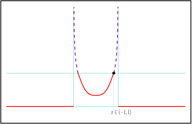
Figure 4. The function $u_{-1/2}$ and the cancellation occurring in (2.24).

A geometric interpretation of (2.24) is depicted in Figure 4 where a point $x\in(-1,1)$ is selected and the graph of $u_{-1/2}$ above the value $u_{-1/2}(x)$ is drawn with a “dashed curve” (while a “solid curve” represents the graph of $u_{-1/2}$ below the value $u_{-1/2}(x)$): then, when computing the fractional Laplacian at $x$, the values coming from the dashed curve, compared with $u_{-1/2}(x)$, provide an opposite sign with respect to the values coming from the solid curve. The “miracle” occurring in (2.24) is that these two contributions with opposite sign perfectly compensate and cancel each other, for any $x\in(-1,1)$.

More generally, in every smooth bounded domain $\Omega\subset\mathbb{R}^{n}$ it is possible to build $s$-harmonic functions exploding at $\partial\Omega$ at the same rate as dist$(\cdot,\partial\Omega)^{s-1}$. A phenomenon of this sort was spotted in [MR2985500], and see [MR3393247] for the explicit explosion rate. See [MR3393247] also for a justification of the boundary behavior, as well as the study of Dirichlet problems prescribing a singular boundary trace.

Concerning this feature of explosive solutions at the boundary, it is interesting to point out a simple analogy with the classical Laplacian. Indeed, in view of (2.15), if $s\in(0,1)$ and we take the function $\mathbb{R}\ni x\mapsto x_{+}^{s}$, we know that it is $s$-harmonic in $(0,+\infty)$ and it vanishes on the boundary (namely, the origin), and these features have a clear classical analogue for $s=1$. Then, since for all $s\in(0,1]$ the derivative of $x_{+}^{s}$ is $x_{+}^{s-1}$, up to multiplicative constants, we have that the latter is $s$-harmonic in $(0,+\infty)$ and it blows-up at the origin when $s\in(0,1)$ (conversely, when $s=1$ one can do the same computations but the resulting function is simply the characteristic function of $(0,+\infty)$ so no explosive effect arises).

Similar computations can be done in the unit ball instead of $(0,+\infty)$, and one simply gets functions that are bounded up to the boundary when $s=1$, or explosive when $s\in(0,1)$ (further details in Appendices G and H).

Difference 2.9 (Decay at infinity).

The Gaussian $e^{-|x|^{2}}$ reproduces the classical heat kernel. That is, the solution of the heat equation with initial datum concentrated at the origin, when considered at time $t=1/4$, produces the Gaussian (of course, the choice $t=1/4$ is only for convenience, any time $t$ can be reduced to unit time by scaling the equation).

The fast decay prescribed by the Gaussian is special for the classical case and the fractional case exhibits power law decays at infinity. More precisely, let us consider the heat equation with initial datum concentrated at the origin, that is

(2.25) $$\left\{\begin{matrix}\partial_{t}u(x,t)=-(-\Delta)^{s}u(x,t)\;{\mbox{ for }}(x,t)\in\mathbb{R}^{n}\times(0,+\infty),\\ u(x,0)=\delta_{0},\end{matrix}\right.$$

and set

(2.26) $${\mathcal{G}}_{s}(x)=u(x,1).$$

By taking the Fourier Transform of (2.25) in the $x$ variable (and possibly neglecting normalization constants) one finds that

$$\left\{\begin{matrix}\partial_{t}\hat{u}=-|\xi|^{2s}\hat{u}\;{\mbox{ in }}\mathbb{R}^{n}\times(0,+\infty),\\ u(\xi,0)=1,\end{matrix}\right.$$

hence

(2.27) $$\hat{u}=e^{-|\xi|^{2s}t},$$

and consequently

(2.28) $${\mathcal{G}}_{s}(x)={\mathcal{F}}^{-1}(e^{-|\xi|^{2s}}),$$

being ${\mathcal{F}}^{-1}$ the anti-Fourier Transform of the Fourier Transform ${\mathcal{F}}$. When $s=1$, and neglecting the normalizing constants, the expression in (2.28) reduces to the Gaussian (since the Gaussian is the Fourier Transform of itself). On the other hand, as far as we know, there is no simple explicit representation of the fractional heat kernel in (2.28), except in the “miraculous” case $s=1/2$, in which (2.28) provides the explicit representation

(2.29) $${\mathcal{G}}_{1/2}(x)=\frac{\,{\rm const}\,}{\big{(}1+|x|^{2}\big{)}^{\frac{n+1}{2}}}.$$

See Appendix I for a proof of (2.29) using Fourier methods and Appendix J for a proof based on extension methods.

We stress that, differently from the classical case, the heat kernel ${\mathcal{G}}_{1/2}$ decays only with a power law. This is in fact a general feature of the fractional case, since, for any $s\in(0,1)$, it holds that

(2.30) $$\lim_{|x|\to+\infty}|x|^{n+2s}{\mathcal{G}}_{s}(x)=\,{\rm const}\,$$

and, for $|x|\geqslant 1$ and $s\in(0,1)$, the heat kernel ${\mathcal{G}}_{s}(x)$ is bounded from below and from above by $\frac{\,{\rm const}\,}{|x|^{n+2s}}$.

We refer to [MR1744782] for a detailed discussion on the fractional heat kernel. See also [MR3211862] for more information on the fractional heat equation. For precise asymptotics on fractional heat kernels, see [zbMATH02598269, MR0119247, MR1297844, 2018arXiv180311435D].

The decay of the heat kernel is also related to the associated distribution in probability theory: as we will see in Section 4.2, the heat kernel represents the probability density of finding a particle at a given point after a unit of time; the motion of such particle is driven by a random walk in the classical case and by a random process with long jumps in the fractional case and, as a counterpart, the fractional probability distribution exhibits a “long tail”, in contrast with the rapidly decreasing classical one.

Another situation in which the classical case provides exponentially fast decaying solutions while the fractional case exhibits polynomial tails is given by the Allen-Cahn equation (see e.g. Section 1.1 in [MR2528756] for a simple description of this equation also in view of phase coexistence models). For concreteness, one can consider the one-dimensional equation

(2.31) $$\left\{\begin{matrix}(-\Delta)^{s}u=u-u^{3}\;{\mbox{ in }}\mathbb{R},\\ \\ \dot{u}>0,\\ u(0)=0,\\ \displaystyle\lim_{t\to\pm\infty}u(t)=\pm 1.\end{matrix}\right.$$

For $s=1$, the system in (2.31) reduces to the pendulum-like system

(2.32) $$\left\{\begin{matrix}-\ddot{u}=u-u^{3}\;{\mbox{ in }}\mathbb{R},\\ \\ \dot{u}>0,\\ u(0)=0,\\ \displaystyle\lim_{t\to\pm\infty}u(t)=\pm 1.\end{matrix}\right.$$

The solution of (2.32) is explicit and it has the form

(2.33) $$u(t):=\tanh\frac{t}{\sqrt{2}},$$

as one can easily check. Also, by inspection, we see that such solution satisfies

(2.34) $$\begin{split}&|u(t)-1|\leqslant\,{\rm const}\,\exp({-\,{\rm const}\,\,t})\quad{\mbox{ for any }}t\geqslant 1\\ {\mbox{and }}\;&|u(t)+1|\leqslant\,{\rm const}\,\exp({-\,{\rm const}\,\,|t|})\quad{\mbox{ for any }}t\leqslant-1.\end{split}$$

Conversely, to the best of our knowledge, the solution of (2.31) has no simple explicit expression. Also, remarkably, the solution of (2.31) decays to the equilibria $\pm 1$ only polynomially fast. Namely, as proved in Theorem 2 of [MR3081641], we have that the solution of (2.31) satisfies

(2.35) $$\begin{split}&|u(t)-1|\leqslant\frac{\,{\rm const}\,}{t^{2s}}\quad{\mbox{ for any }}t\geqslant 1\\ {\mbox{and }}\;&|u(t)+1|\leqslant\frac{\,{\rm const}\,}{|t|^{2s}}\quad{\mbox{ for any }}t\leqslant-1,\end{split}$$

and the estimates in (2.35) are optimal, namely it also holds that

(2.36) $$\begin{split}&|u(t)-1|\geqslant\frac{\,{\rm const}\,}{t^{2s}}\quad{\mbox{ for any }}t\geqslant 1\\ {\mbox{and }}\;&|u(t)+1|\geqslant\frac{\,{\rm const}\,}{|t|^{2s}}\quad{\mbox{ for any }}t\leqslant-1.\end{split}$$

See Appendix K for a proof of (2.36). In particular, (2.36) says that solutions of fractional Allen-Cahn equations such as the one in (2.31) do not satisfy the exponential decay in (2.34) which is fulfilled in the classical case.

The estimate in (2.36) can be confirmed by looking at the solution of the very similar equation

(2.37) $$\left\{\begin{matrix}(-\Delta)^{s}u=\displaystyle\frac{1}{\pi}\sin(\pi u)\;{\mbox{ in }}\mathbb{R},\\ \\ \dot{u}>0,\\ u(0)=0,\\ \displaystyle\lim_{t\to\pm\infty}u(t)=\pm 1.\end{matrix}\right.$$

Though a simple expression of the solution of (2.37) is not available in general, the “miraculous” case $s=1/2$ possesses an explicit solution, given by

(2.38) $$u(t):=\frac{2}{\pi}\,\arctan t.$$

That (2.38) is a solution of (2.37) when $s=1/2$ is proved in Appendix L. Another proof of this fact using (2.29) is given in Appendix M.

The reader should not be misled by the similar typographic forms of (2.33) and (2.38), which represent two very different behaviors at infinity: indeed

$$\lim_{t\to+\infty}t\,\left(1-\frac{2}{\pi}\,\arctan t\right)=\frac{2}{\pi},$$

and the function in (2.38) satisfies the slow decay in (2.36) (with $s=1/2$) and not the exponentially fast one in (2.34).

Equations like the one in (2.31) naturally arise, for instance, in long-range phase coexistence models and in models arising in atom dislocation in crystals, see e.g. [MR1442163, MR3296170].

A similar slow decay also occurs in the study of fractional Schrödinger operators, see e.g. [MR1054115] and Lemma C.1 in [MR3530361]. For instance, the solution of

(2.39) $$(-\Delta)^{s}\Gamma+\Gamma=\delta_{0}\quad{\mbox{ in }}\delta_{0}$$

satisfies, for any $|x|\geqslant 1$,

$$\Gamma(x)\simeq\frac{\,{\rm const}\,}{|x|^{n+2s}}.$$

A heuristic motivation for a bound of this type can be “guessed” from (2.39) by thinking that, for large $|x|$, the function $\Gamma$ should decay more or less like $(-\Delta)^{s}\Gamma$, which has “typically” the power law decay described in (2.10).

If one wishes to keep arguing in this heuristic way, also the decays in (2.30) and (2.36) may be seen as coming from an interplay between the right and the left side of the equation, in the light of the decay of the fractional Laplace operator discussed in (2.10). For instance, to heuristically justify (2.30), one may think that the solution of the fractional heat equation which starts from a Dirac’s Delta, after a unit of time (or an “infinitesimal unit” of time, if one prefers) has produced some bump, whose fractional Laplacian, in view of (2.10), may decay at infinity like $\frac{1}{|x|^{n+2s}}$. Since the time derivative of the solution has to be equal to that, the solution itself, in this unit of time, gets “pushed up” by an amount like $\frac{1}{|x|^{n+2s}}$ with respect to the initial datum, thus justifying (2.30).

A similar justification for (2.36) may seem more tricky, since the decay in (2.36) is only of the type $\frac{1}{|t|^{2s}}$ instead of $\frac{1}{|t|^{1+2s}}$, as the analysis in (2.10) would suggest. But to understand the problem, it is useful to consider the derivative of the solution $v:=\dot{u}$ and deduce from (2.31) that

(2.40) $$(-\Delta)^{s}v=(-\Delta)^{s}\dot{u}=\dot{u}-3u^{2}\dot{u}=(1-3u^{2})v.$$

That is, for large $|t|$, the term $1-3u^{2}$ gets close to $1-3=-2$ and so the profile at infinity may locally resemble the one driven by the equation $(-\Delta)^{s}v=-2v$. In this range, $v$ has to balance its fractional Laplacian, which is expected to decay like $\frac{1}{|t|^{1+2s}}$, in view of (2.10). Then, since $u$ is the primitive of $v$, one may expect that its behavior at infinity is related to the primitive of $\frac{1}{|t|^{1+2s}}$, and so to $\frac{1}{|t|^{2s}}$, which is indeed the correct answer given by (2.36).

We are not attempting here to make these heuristic considerations rigorous, but perhaps these kinds of comments may be useful in understanding why the behavior of nonlocal equations is different from that of classical equations and to give at least a partial justification of the delicate quantitative aspects involved in a rigorous quantitative analysis (in any case, ideas like these are rigorously exploited for instance in Appendix K).

See also [MR3461371] for decay estimates of ground states of a nonlinear nonlocal problem.

We also mention that other very interesting differences in the decay of solutions arise in the study of different models for fractional porous medium equations, see e.g. [MR2737788, MR2773189, MR3082241].

Difference 2.10 (Finiteness versus infiniteness of the mean squared displacement).

The mean squared displacement is a useful notion to measure the “speed of a diffusion process”, or more precisely the portion of the space that gets “invaded” at a given time by the spreading of the diffusive quantity which is concentrated at a point source at the initial time. In a formula, if $u(x,t)$ is the fundamental solution of the diffusion equation related to the diffusion operator $\textswab{L}$, namely

(2.41) $$\left\{\begin{matrix}\partial_{t}u=\textswab{L}u&{\mbox{ for any $x\in\mathbb{R}^{n}$ and $t>0$}},\\ u(\cdot,0)=\delta_{0}(\cdot),\end{matrix}\right.$$

being $\delta_{0}$ the Dirac’s Delta, one can define the mean squared displacement relative to the diffusion process $\textswab{L}$ as the “second moment” of $u$ in the space variables, that is

(2.42) $${\rm MSD}_{\textswab{L}}(t):=\int_{\mathbb{R}^{n}}|x|^{2}\,u(x,t)\,dx.$$

For the classical heat equation, by Fourier Transform one sees that, when $\textswab{L}=\Delta$, the fundamental solution of (2.41) is given by the classical heat kernel

$$u(x,t)={\frac{1}{(4\pi t)^{n/2}}}e^{-\frac{|x|^{2}}{4t}},$$

and therefore in such case, the substitution $y:=\frac{x}{2\sqrt{t}}$ gives that

(2.43) $${\rm MSD}_{\Delta}(t)=\int_{\mathbb{R}^{n}}{\frac{|x|^{2}}{(4\pi t)^{n/2}}}e^{-\frac{|x|^{2}}{4t}}\,dx=\int_{\mathbb{R}^{n}}{\frac{4t|y|^{2}}{\pi^{n/2}}}e^{-|y|^{2}}\,dy=Ct,$$

for some $C>0$. This says that the mean squared displacement of the classical heat equation is finite, and linear in the time variable.

On the other hand, in the fractional case in which $\textswab{L}=-(-\Delta)^{s}$, by (2.27) the fractional heat kernel is endowed with the scaling property

$$u(x,t)=\frac{1}{t^{\frac{n}{2s}}}{\mathcal{G}}_{s}\left(\frac{x}{t^{\frac{1}{2s}}}\right),$$

with ${\mathcal{G}}_{s}$ being as in (2.25) and (2.26). Consequently, in this case, the substitution $y:=\frac{x}{t^{\frac{1}{2s}}}$ gives that

(2.44) $${\rm MSD}_{-(-\Delta)^{s}}(t)=\int_{\mathbb{R}^{n}}|x|^{2}\,\frac{1}{t^{\frac{n}{2s}}}{\mathcal{G}}_{s}\left(\frac{x}{t^{\frac{1}{2s}}}\right)\,dx=t^{\frac{1}{s}}\,\int_{\mathbb{R}^{n}}|y|^{2}\,{\mathcal{G}}_{s}(y)\,dy.$$

Now, from (2.30), we know that

$$\int_{\mathbb{R}^{n}}|y|^{2}\,{\mathcal{G}}_{s}(y)\,dy=+\infty$$

and therefore we infer from (2.44) that

(2.45) $${\rm MSD}_{-(-\Delta)^{s}}(t)=+\infty.$$

This computation shows that, when $s\in(0,1)$, the diffusion process induced by $-(-\Delta)^{s}$ does not possess a finite mean squared displacement, in contrast with the classical case in (2.43).

Other important differences between the classical and fractional cases arise in the study of nonlocal minimal surfaces and in related fields: just to list a few features, differently than in the classical case, nonlocal minimal surfaces typically “stick” at the boundary, see [MR3516886, MR3596708, POICLA], the gradient bounds of nonlocal minimal graphs are different than in the classical case, see [DUCA], nonlocal catenoids grow linearly and nonlocal stable cones arise in lower dimension, see [LAWSON, 2018arXiv181112141C], stable surfaces of vanishing nonlocal mean curvature possess uniform perimeter bounds, see Corollary 1.8 in [BVSUP], the nonlocal mean curvature flow develops singularity also in the plane, see [SIN], its fattening phenomena are different, see [FATTE], and the self-shrinking solutions are also different, see [2018arXiv181201847C], and genuinely nonlocal phase transitions present stronger rigidity properties than in the classical case, see e.g. Theorem 1.2 in [owduir375957973] and [FOFISEA]. Furthermore, from the probabilistic viewpoint, recurrence and transiency in long-jump stochastic processes are different from the case of classical random walks, see e.g. [AFFILI] and the references therein.

We would like to conclude this list of differences with one similarity, which seems to be not very well-known. There is indeed a “nonlocal representation” for the classical Laplacian in terms of a singular kernel. It reads as

(2.46) $$-\Delta u(x)=\,{\rm const}\,\int_{\mathbb{R}^{n}}\frac{u(x+2y)+u(x-2y)-4u(x+y)-4u(x-y)+6u(x)}{{|y|}^{n+2}}\;dy.$$

This one is somehow very close to (2.2) with one important modification: the difference operator in the numerator of the integrand has been increased in order, in such a way that it is able to compensate the singularity of the kernel in $0$. We include in Appendix N a computation proving (2.46) when $u$ is $C^{2,\alpha}$ around $x$. For a complete proof, involving Fourier transform techniques and providing the explicit value of the constant, we refer to [AJS1].

2.2. The regional (or censored) fractional Laplacian

A variant of the fractional Laplacian in (2.1) consists in restricting the domain of integration to a subset of $\mathbb{R}^{n}$. In this direction, an interesting operator is defined by the following singular integral:

(2.47) $$(-\Delta)^{s}_{\Omega}u(x):=\,{\rm P.V.}\,\int_{\Omega}\frac{u(x)-u(y)}{|x-y|^{n+2s}}\,dy.$$

We remark that when $\Omega:=\mathbb{R}^{n}$ the regional fractional Laplacian in (2.47) boils down to the standard fractional Laplacian in (2.1).

In spite of the apparent similarity, the regional fractional Laplacian and the fractional Laplacian are structurally two different operators. For instance, concerning Difference 2.4, we mention that solutions of regional fractional Laplace equations do not possess the same rich structure of those of fractional Laplace equations, and indeed

(2.48) $$\begin{split}&{\mbox{it is not true that for any\leavevmode\nobreak\ $\varepsilon>0$ and any (bounded, smooth) function\leavevmode\nobreak\ $\bar{u}$,}}\\ &{\mbox{we can find\leavevmode\nobreak\ $v_{\varepsilon}$ such that}}\\ &\left\{\begin{matrix}\|\bar{u}-v_{\varepsilon}\|_{C^{2}(B_{1})}\leqslant\varepsilon\\ {\mbox{and }}(-\Delta)^{s}_{\Omega}v_{\varepsilon}=0{\mbox{ in }}B_{1}.\end{matrix}\right.\end{split}$$

A proof of this observation will be given in Appendix O.

Interestingly, the regional fractional Laplacian turns out to be useful also in a possible setting of Neumann-type conditions in the nonlocal case, as presented in [MR3651008]. Related to this, we mention that it is possible to obtain a regional-type operator starting from the classical Laplacian coupled with Neumann boundary conditions (details about it will be given in formula (2.52) below).

2.3. The spectral fractional Laplacian

Another natural fractional operator arises in taking fractional powers of the eigenvalues. For this, we write

(2.49) $$u(x,t)=\sum_{k=0}^{+\infty}u_{k}(t)\,\phi_{k}(x),$$

where $\phi_{k}$ is the eigenfunction corresponding to the $k$th eigenvalue of the Dirichlet Laplacian, namely

$$\left\{\begin{matrix}-\Delta\phi_{k}=\lambda_{k}\phi_{k}{\mbox{ in }}\Omega\\ \phi_{k}\in H^{1}_{0}(\Omega).\end{matrix}\right.$$

with $0<\lambda_{0}<\lambda_{1}\leqslant\lambda_{2}\leqslant\dots$. We normalize the sequence $\phi_{k}$ to make it an orthonormal basis of $L^{2}(\Omega)$ (see e.g. page 335 in [MR1625845]). In this setting, we define

(2.50) $$(-\Delta)^{s}_{D,\Omega}u(x):=\sum_{k=0}^{+\infty}{\lambda_{k}^{s}}\,u_{k}(t)\,\phi_{k}(x).$$

We refer to [MR2754080] for extension methods for this type of operator. Furthermore, other types of fractional operators can be defined in terms of different boundary conditions: for instance, a spectral decomposition with respect to the eigenfunctions of the Laplacians with Neumann boundary data naturally leads to an operator $(-\Delta)^{s}_{N,\Omega}$ (and such operator also have applications in biology, see e.g. [MR3082317] and [SOA]).

It is also interesting to observe that the spectral fractional Laplacian with Neumann boundary conditions can also be written in terms of a regional operator with a singular kernel. Namely, given an open and bounded set $\Omega\subset\mathbb{R}^{n}$, denoting by ${\Delta_{N,\Omega}}$ the Laplacian operator coupled with Neumann boundary conditions on $\partial\Omega$, we let ${\{(\mu_{j},\psi_{j})\}}_{j\in\mathbb{N}}$ the pairs made up of eigenvalues and eigenfunctions of ${-\Delta_{N,\Omega}}$, that is

$$\left\{\begin{matrix}-\Delta\psi_{j}=\mu_{j}\psi_{j}{\mbox{ in }}\Omega\\ \partial_{\nu}\psi_{j}=0\text{ on }\partial\Omega\\ \psi_{j}\in H^{1}(\Omega).\end{matrix}\right.$$

with $0=\mu_{0}<\mu_{1}\leqslant\mu_{2}\leqslant\mu_{3}\leqslant\dots$.

We define the following operator by making use of a spectral decomposition

(2.51) $${(-\Delta)^{s}_{N,\Omega}}\ :=\ \sum_{j=0}^{+\infty}\mu_{j}^{s}\hat{u}_{j}\>\psi_{j},\qquad\hat{u}_{j}=\int_{\Omega}u\psi_{j},\ u\in C^{\infty}_{0}(\Omega).$$

Comparing with (2.50), we can consider $(-\Delta)^{s}_{N,\Omega}$ a spectral fractional Laplacian with respect to classical Neumann data. In this setting, the operator $(-\Delta)^{s}_{N,\Omega}$ is also an integrodifferential operator of regional type, in the sense that one can write

(2.52) $$(-\Delta)^{s}_{N,\Omega}u(x)=\,{\rm P.V.}\,\int_{\Omega}\big{(}u(x)-u(y)\big{)}\,K(x,y)\,dy,$$

for a kernel $K(x,y)$ which is comparable to $\frac{1}{|x-y|^{n+2s}}$. We refer to Appendix P for a proof of this.

Interestingly, the fractional Laplacian and the spectral fractional Laplacian coincide, up to a constant, for periodic functions, or functions defined on the flat torus, namely

(2.53) if $$u(x+k)=u(x) x\in\mathbb{R}^{n} k\in\mathbb{Z}^{n} (-\Delta)^{s}_{D,\Omega}u(x)=\,{\rm const}\,(-\Delta)^{s}u(x)$$ for any  and , then .

See e.g. Appendix Q for a proof of this fact.

On the other hand, striking differences between the fractional Laplacian and the spectral fractional Laplacian hold true, see e.g. [MR3233760, MR3246044].

Interestingly, it is not true that all functions are $s$-harmonic with respect to the spectral fractional Laplacian, up to a small error, that is

(2.54) $$\begin{split}&{\mbox{it is not true that for any\leavevmode\nobreak\ $\varepsilon>0$ and any (bounded, smooth) function\leavevmode\nobreak\ $\bar{u}$,}}\\ &{\mbox{we can find\leavevmode\nobreak\ $v_{\varepsilon}$ such that}}\\ &\left\{\begin{matrix}\|\bar{u}-v_{\varepsilon}\|_{C^{2}(B_{1})}\leqslant\varepsilon\\ {\mbox{and }}(-\Delta)^{s}_{D,\Omega}v_{\varepsilon}=0{\mbox{ in }}B_{1}.\end{matrix}\right.\end{split}$$

A proof of this will be given in Appendix R. The reader can easily compare (2.54) with the setting for the fractional Laplacian discussed in Difference 2.4.

Remarkably, in spite of these differences, the spectral fractional Laplacian can also be written as an integrodifferential operator of the form

(2.55) $$\,{\rm P.V.}\,\int_{\Omega}\big{(}u(x)-u(y)\big{)}\,K(x,y)\,dy+\beta(x)u(x),$$

for a suitable kernel $K$ and potential $\beta$, see Lemma 38 in [MR3610940] or Lemma 10.1 in [2016arXiv161009881B]. This can be proved with analogous computations to those performed in the case of the regional fractional Laplacian in the previous paragraph.

2.4. Fractional time derivatives

The operators described in Sections in 2.1, 2.2 and 2.3 are often used in the mathematical description of anomalous types of diffusion (i.e. diffusive processes which produce important differences with respect to the classical heat equation, as we will discuss in Section 4): the main role of such nonlocal operators is usually to produce a different behavior of the diffusion process with respect to the space variables.

Other types of anomalous diffusions arise from non-standard behaviors with respect to the time variable. These aspects are often the mathematical counterpart of memory effects. As a prototype example, we recall the notion of Caputo fractional derivative, which, for any $t>0$ (and up to normalizing factors that we omit for simplicity) is given by

(2.56) $$\partial^{s}_{C,t}u(t):=\int_{0}^{t}\frac{\dot{u}(\tau)}{(t-\tau)^{s}}\,d\tau.$$

We point out that, for regular enough functions $u$,

(2.57) $$\begin{split}\partial^{s}_{C,t}u(t)\,&=\int_{0}^{t}\frac{\dot{u}(\tau)}{(t-\tau)^{s}}\,d\tau\\ &=\int_{0}^{t}\left(\frac{d}{d\tau}\frac{\big{(}u(\tau)-u(t)\big{)}}{(t-\tau)^{s}}-s\,\frac{\big{(}u(\tau)-u(t)\big{)}}{(t-\tau)^{1+s}}\right)\,d\tau\\ &=\frac{u(t)-u(0)}{t^{s}}-\lim_{\tau\to t}\frac{u(t)-u(\tau)}{(t-\tau)^{s}}-s\,\int_{0}^{t}\frac{\big{(}u(\tau)-u(t)\big{)}}{(t-\tau)^{1+s}}\,d\tau\\ &=\frac{u(t)-u(0)}{t^{s}}-\dot{u}(t)\,\lim_{\tau\to t}(t-\tau)^{1-s}-s\,\int_{0}^{t}\frac{u(\tau)-u(t)}{(t-\tau)^{1+s}}\,d\tau\\ &=\frac{u(t)-u(0)}{t^{s}}+s\,\int_{0}^{t}\frac{u(t)-u(\tau)}{(t-\tau)^{1+s}}\,d\tau.\end{split}$$

Though in principle this expression takes into account only the values of $u(t)$ for $t\geqslant 0$, hence $u$ does not need to be defined for negative times, as pointed out e.g. in Section 2 of [MR3488533], it may be also convenient to constantly extend $u$ in $(-\infty,0)$. Hence, we take the convention for which $u(t)=u(0)$ for any $t\leqslant 0$. With this extension, one has that, for any $t>0$,

$$s\,\int_{-\infty}^{0}\frac{u(t)-u(\tau)}{(t-\tau)^{1+s}}\,d\tau=s\,\int_{-\infty}^{0}\frac{u(t)-u(0)}{(t-\tau)^{1+s}}\,d\tau=\frac{u(t)-u(0)}{t^{s}}.$$

Hence, one can write (2.57) as

(2.58) $$\partial^{s}_{C,t}u(t)=s\,\int_{-\infty}^{t}\frac{u(t)-u(\tau)}{(t-\tau)^{1+s}}\,d\tau.$$

This type of formulas also relates the Caputo derivative to the so-called Marchaud derivative, see e.g. [MR1347689].

In the literature, one can also consider higher order Caputo derivatives, see e.g. [MR2090004, MR1829592] and the references therein.

Also, it is useful to consider the Caputo derivative in light of the (unilateral) Laplace Transform (see e.g. Chapter 2.8 in [MR1658022], and [iqo0eiKAL])

(2.59) $${\mathcal{L}}u(\omega):=\int_{0}^{+\infty}u(t)\,e^{-\omega t}\,dt.$$

With this notation, up to dimensional constants, one can write (for a smooth function with exponential control at infinity) that

(2.60) $${\mathcal{L}}(\partial^{s}_{C,t}u)(\omega)=\omega^{s}{\mathcal{L}}u(\omega)-\omega^{s-1}u(0),$$

see Appendix S for a proof.

In this way, one can also link equations driven by the Caputo derivative to the so-called Volterra integral equations: namely one can invert the expression $\partial^{s}_{C,t}u=f$ by

(2.61) $$u(t)=u(0)+C\int_{0}^{t}\frac{f(\tau)}{(t-\tau)^{1-s}}\,d\tau,$$

for some normalization constant $C>0$, see Appendix T for a proof.

It is also worth mentioning that the Caputo derivative of order $s$ of a power gives, up to normalizing constants, the “power minus $s$”: more precisely, by (2.56) and using the substitution $\vartheta:=\tau/t$, we see that, for any $r>0$,

$$\partial^{s}_{C,t}(t^{r})=r\,\int_{0}^{t}\frac{\tau^{r-1}}{(t-\tau)^{s}}\,d\tau=r\,t^{r-s}\,\int_{0}^{1}\frac{\vartheta^{r-1}}{(1-\vartheta)^{s}}\,d\vartheta=Ct^{r-s},$$

for some $C>0$.

Moreover, in relation to the comments on page 2.41, we have that

(2.62) $$\begin{split}&{\mbox{the mean squared displacement related to the diffusion operator}}\\ &\left\{\begin{matrix}\partial^{s}_{C,t}u=\Delta u&{\mbox{ for any $x\in\mathbb{R}^{n}$ and $t>0$}},\\ u(\cdot,0)=\delta_{0}(\cdot),\end{matrix}\right.\\ &{\mbox{is finite and proportional to\leavevmode\nobreak\ $t^{s}$}}.\end{split}$$

See Appendix U for a proof of this.

The Caputo derivatives describes a process “with memory”, in the sense that it “remembers the past”, though “old events count less than recent ones”. We sketch a memory effect of Caputo type in Appendix V.

Due to its memory effect, operators related to Caputo derivatives have found several applications in which the basic parameters of a physical system change in time, in view of the evolution of the system itself: for instance, in studying flows in porous media, when time goes, the fluid may either “obstruct” the holes of the medium, thus slowing down the diffusion, or “clean” the holes, thus making the diffusion faster, and the Caputo derivative may be a convenient approach to describe such modification in time of the diffusion coefficient, see [MR2379269].

Other applications of Caputo derivatives occur in biology and neurosciences, since the network of neurons exhibit time-fractional diffusion, also in view of their highly ramified structure, see e.g. [PuPOw2e3we] and the references therein.

We also refer to [MR3469920, MR3177769, 2017arXiv170608241V] and to the references therein for further discussions on different types of anomalous diffusions.

3. A more general point of view: the “master equation”

The operators discussed in Sections 2.1, 2.2, 2.3 and 2.4 can be framed into a more general setting, that is that of the “master equation”, see e.g. [MR3329847].

Master equations describe the evolution of a quantity in terms of averages in space and time of the quantity itself. For concreteness one can consider a quantity $u=u(x,t)$ and describe its evolution by an equation of the kind

$$c\partial_{t}u(x,t)=Lu(x,t)+f\big{(}x,t,u(x,t)\big{)}$$

for some $c\in\mathbb{R}$ and a forcing term $f$, and the operator $L$ has the integral form

(3.1) $$Lu(x,t):=\iint_{\mathbb{R}^{n}\times(0,+\infty)}\big{(}u(x,t)-u(x-y,t-\tau)\big{)}\,{\mathcal{K}}(x,t,y,\tau)\,d\mu(x,\tau),$$

for a suitable measure $\mu$ (with the integral possibly taken in the principal value sense, which is omitted here for simplicity; also one can consider even more general operators by taking actions different than translations and more general ambient spaces).

Though the form of such operator is very general, one can also consider simplifying structural assumptions. For instance, one can take $\mu$ to be the space-time Lebesgue measure over $\mathbb{R}^{n}\times(0,+\infty)$, namely

$$d\mu(x,\tau)=dx\,d\tau.$$

Another common simplifying assumption is to assume that the kernel is induced by an uncorrelated effect of the space and time variables, with the product structure

$${\mathcal{K}}(x,t,y,\tau)={\mathcal{K}}_{\rm space}(x,y)\,{\mathcal{K}}_{\rm time}(t,\tau).$$

The fractional Laplacian of Section 2.1 is a particular case of this setting (for functions depending on the space variable), with the choice, up to normalizing constants,

$${\mathcal{K}}_{\rm space}(x,y):=\frac{1}{|y|^{n+2s}}.$$

More generally, for $\Omega\subseteq\mathbb{R}^{n}$, the regional fractional Laplacian in Section 2.2 comes from the choice

$${\mathcal{K}}_{\rm space}(x,y):=\frac{\chi_{\Omega}(x-y)}{|y|^{n+2s}}.$$

Finally, in view of (2.58), for time-dependent functions, the choice

$${\mathcal{K}}_{\rm time}(t,\tau):=\frac{\chi_{(-\infty,t)}(\tau)}{|\tau|^{1+s}}.$$

produces the Caputo derivative discussed in Section 2.4.

We recall that one of the fundamental structural differences in partial differential equations consists in the distinction between operators “in divergence form”, such as

(3.2) $$-\sum_{i,j=1}^{n}\frac{\partial}{\partial x_{i}}\left(a_{ij}(x)\frac{\partial u}{\partial x_{j}}(x)\right)$$

and those “in non-divergence form”, such as

(3.3) $$-\sum_{i,j=1}^{n}a_{ij}(x)\frac{\partial^{2}u}{\partial x_{i}\partial x_{j}}(x).$$

This structural difference can also be recovered from the master equation. Indeed, if we consider a (say, for the sake of concreteness, strictly positive, bounded and smooth) matrix function $M:\mathbb{R}^{n}\to{\rm Mat}(n\times n)$, we can take into account the master spatial operator induced by the kernel

(3.4) $${\mathcal{K}}_{\rm space}(x,y):=\frac{1-s}{|M(x-y,y)\,y|^{n+2s}},$$

that is, in the notation of (3.1),

(3.5) $$(1-s)\,\int_{\mathbb{R}^{n}}\frac{u(x)-u(x-y)}{|M(x-y,y)\,y|^{n+2s}}\,dy.$$

Then, up to a normalizing constant, if

(3.6) $$M(x-y,y)=M(x,-y),$$

then

(3.7) $$\begin{split}&{\mbox{the limit as\leavevmode\nobreak\ $s\nearrow 1$ of the operator in\leavevmode\nobreak\ \eqref{DIU8234j:3}}}\\ &{\mbox{recovers the classical divergence form operator in\leavevmode\nobreak\ \eqref{DIU8234j:1},}}\\ &{\mbox{with }}a_{ij}(x):=\,{\rm const}\,\int_{S^{n-1}}\frac{\omega_{i}\,\omega_{j}}{|M(x,0)\,\omega|^{n+2}}\,d{\mathcal{H}}^{n-1}_{\omega}.\end{split}$$

A proof of this will be given in Appendix W.

It is interesting to observe that condition (3.6) says that, if we set $z:=x-y$, then

(3.8) $$M(z,x-z)=M(x,z-x)$$

and so the kernel in (3.4) is invariant by exchanging $x$ and $z$. This invariance naturally leads to a (possibly formal) energy functional of the form

(3.9) $$\frac{1-s}{2}\,\iint_{\mathbb{R}^{n}\times\mathbb{R}^{n}}\frac{\big{(}u(x)-u(z)\big{)}^{2}}{|M(z,x-z)\,(x-z)|^{n+2s}}\,dx\,dz.$$

We point out that condition (3.8) translates, roughly speaking, into the fact that the energy density in (3.9) “charges the variable $x$ as much as the variable $z$”.

The study of the energy functional in (3.9) also drives to a natural quasilinear generalization, in which the fractional energy takes the form

$$\int_{\mathbb{R}^{n}}\frac{\Phi\big{(}u(x)-u(z)\big{)}}{|M(z,x-z)\,(x-z)|^{n+2s}}\,dx\,dz,$$

for a suitable $\Phi$, see e.g. [MR3339179, MR3456825] and the references therein for further details on quasilinear nonlocal operators. See also [MR3177769] and the references therein for other type of nonlinear fractional equations.

Another case of interest (see e.g. [MR1918242]) is the one in which one considers the master equation driven by the spatial kernel

$${\mathcal{K}}_{\rm space}(x,y):=\frac{1-s}{|M(x,y)\,y|^{n+2s}}\,dy,$$

that is, in the notation of (3.1),

(3.10) $$(1-s)\,\int_{\mathbb{R}^{n}}\frac{u(x)-u(x-y)}{|M(x,y)\,y|^{n+2s}}\,dy.$$

Then, up to a normalizing constant, if

(3.11) $$M(x,y)=M(x,-y),$$

then

(3.12) $$\begin{split}&{\mbox{the limit as\leavevmode\nobreak\ $s\nearrow 1$ of the operator in\leavevmode\nobreak\ \eqref{DIU8234j:4}}}\\ &{\mbox{recovers the classical non-divergence form operator in\leavevmode\nobreak\ \eqref{DIU8234j:2},}}\\ &{\mbox{with }}a_{ij}(x):=\,{\rm const}\,\int_{S^{n-1}}\frac{\omega_{i}\omega_{j}}{|M(x,0)\,\omega|^{n+2}}\,d{\mathcal{H}}^{n-1}_{\omega}\end{split}$$

A proof of this will be given in Appendix X.

We recall that nonlocal linear operators in non-divergence form can also be useful in the definition of fully nonlinear nonlocal operators, by taking appropriate infima and suprema of combinations of linear operators, see e.g. [MR3148110] and the references therein for further discussions about this topic (which is also related to stochastic games).

We also remark that understanding the role of the affine transformations of the spaces on suitable nonlocal operators (as done for instance in (3.10) and (3.10)) often permits a deeper analysis of the problem in nonlinear settings too, see e.g. the very elegant way in which a fractional Monge-Ampère equation is introduced in [MR3479063] by considering the infimum of fractional linear operators corresponding to all affine transformations of determinant one of a given multiple of the fractional Laplacian.

As a general comment, we also think that an interesting consequence of the considerations given in this section is that classical, local equations can also be seen as a limit approximation of more general master equations.

We mention that there are also many other interesting kernels, both in space and time, which can be taken into account in integral equations. Though we focused here mostly on the case of singular kernels, there are several important problems that focus on “nice” (e.g. integrable) kernels, see e.g. [MR2722295, MR2958346, MR3641640] and the references therein.

As a technical comment let us point out that, in a sense, the nice kernels may have computational advantages, but may provide loss of compactness and loss of regularity issues: roughly speaking, convolutions with smooth kernel are always smooth, thus any smoothness information on a convolved function gives little information on the smoothness of the original function – viceversa, if the convolution of an “object” with a singular kernel is smooth, then it means that the original object has a “good order of vanishing at the origin”. When the original object is built by the difference of a function and its translation, such vanishing implies some control of the oscillation of the function, hence opening a door towards a regularity result.

4. Probabilistic motivations

We provide here some elementary, and somewhat heuristic, motivations for the operators described in Section 2 in view of probability and statistics applications. The treatment of this section is mostly colloquial and not to be taken at a strictly rigorous level (in particular, all functions are taken to be smooth, some uniformity problems are neglected, convergence is taken for granted, etc.). See e.g. [MR1409607] for rigorous explanations linking pseudo-differential operators and Markov/Lévy processes. See also [MR1406564, MR2345912, MR2512800, MR2584076, MR2963050] for other perspectives and links between probability and fractional calculus and [K201717] for a complete survey on jump processes and their connection to nonlocal operators.

The probabilistic approach to study nonlocal effects and the analysis of distributions with polynomial tails are also some of the cornerstones of the application of mathematical theories to finance, see e.g. [PARETO, MANDEL], and models with jump process for prices have been proposed in [COX].

4.1. The heat equation and the classical Laplacian

The prototype of parabolic equations is the heat equation

(4.1) $$\partial_{t}u(x,t)=c\,\Delta u(x,t)$$

for some $c>0$. The solution $u$ may represent, for instance, a temperature, and the foundation of (4.1) lies on two basic assumptions:

• the variation of $u$ in a given region $U\subset\mathbb{R}^{n}$ is due to the flow of some quantity $v:\mathbb{R}^{n}\to\mathbb{R}^{n}$ through $U$,

• $v$ is produced by the local variation of $u$.

The first ansatz can be written as

(4.2) $$\partial_{t}\int_{U}u(y,t)\,dy=\int_{\partial U}v(y,t)\cdot\nu(y)\,d{\mathcal{H}}^{n-1}_{y},$$

where $\nu$ denotes the exterior normal vector of $U$ and ${\mathcal{H}}^{n-1}$ is the standard $(n-1)$-dimensional surface Hausdorff measure.

The second ansatz can be written as $v=c\nabla u$, which combined with (4.2) and the Divergence Theorem gives that

$$\partial_{t}\int_{U}u(y,t)\,dy=c\int_{\partial U}\nabla u(y,t)\cdot\nu(y)\,d{\mathcal{H}}^{n-1}_{y}=c\int_{U}{\rm div}\,(\nabla u(y,t))\,dy=c\int_{U}\Delta u(y,t)\,dy.$$

Since $U$ is arbitrary, this gives (4.1).

Let us recall a probabilistic interpretation of (4.1). The idea is that (4.1) follows by taking suitable limits of a discrete “random walk”. For this, we take a small space scale $h>0$ and a time step

(4.3) $$\tau=h^{2}.$$

We consider the random motion of a particle in the lattice $h\mathbb{Z}^{n}$, as follows. At each time step, the particle can move in any coordinate direction with equal probability. That is, a particle located at $h\bar{k}\in h\mathbb{Z}^{n}$ at time $t$ is moved to one of the $2n$ points $h\bar{k}\pm he_{1}$, $\dots$, $h\bar{k}\pm he_{n}$ with equal probability (here, as usual, $e_{j}$ denotes the $j$th element of the standard Euclidean basis of $\mathbb{R}^{n}$).

We now look at the expectation to find the particle at a point $x\in h\mathbb{Z}^{n}$ at time $t\in\tau\mathbb{N}$. For this, we denote by $u(x,t)$ the probability density of such expectation. That is, the probability for the particle of lying in the spatial region $B_{r}(x)$ at time $t$ is, for small $r$, comparable with

$$\int_{B_{r}(x)}u(y,t)\,dy.$$

Then, the probability of finding a particle at the point $x\in h\mathbb{Z}^{n}$ at time $t+\tau$ is the sum of the probabilities of finding the particle at a closest neighborhood of $x$ at time $t$, times the probability of jumping from this site to $x$. That is,

(4.4) $$u(x,t+\tau)=\frac{1}{2n}\sum_{j=1}^{n}\Big{(}u(x+he_{j})+u(x-he_{j})\Big{)}.$$

Also,

$$u(x+he_{j})+u(x-he_{j})-2u(x,t)$$

$$= \left(u(x,t)+h\nabla u(x,t)\cdot e_{j}+\frac{h^{2}\,D^{2}u(x,t)\,e_{j}\cdot e_{j}}{2}\right)+\left(u(x,t)-h\nabla u(x,t)\cdot e_{j}+\frac{h^{2}\,D^{2}u(x,t)\,e_{j}\cdot e_{j}}{2}\right)$$

$$\qquad-2u(x,t)+O(h^{3})$$

$$= h^{2}\,\partial^{2}_{x_{j}}u(x,t)+O(h^{3}).$$

Thus, subtracting $u(x,t)$ to both sides in (4.4), dividing by $\tau$, recalling (4.3), and taking the limit (and neglecting any possible regularity issue), we formally find that

$$\partial_{t}u(x,t) = \lim_{\tau\searrow 0}\frac{u(x,t+\tau)-u(x,t)}{\tau}$$

$$= \lim_{h\searrow 0}\frac{1}{2n}\sum_{j=1}^{n}\frac{u(x+he_{j})+u(x-he_{j})-2u(x,t)}{h^{2}}$$

$$= \lim_{h\searrow 0}\frac{1}{2n}\sum_{j=1}^{n}\partial^{2}_{x_{j}}u(x,t)+O(h)$$

$$= \frac{1}{2n}\Delta u(x,t),$$

which is (4.1).

4.2. The fractional Laplacian and the regional fractional Laplacian

Now we consider an open set $\Omega\subseteq\mathbb{R}^{n}$ and a discrete random process in $h\mathbb{Z}^{n}$ which can be roughly speaking described in this way. The space parameter $h>0$ is linked to the time step

(4.5) $$\tau:=h^{2s}.$$

A particle starts its journey from a given point $h\bar{k}\in\Omega$ of the lattice $h\mathbb{Z}^{n}$ and, at each time step $\tau$, it can reach any other point of the lattice $hk$, with $k\neq\bar{k}$, with probability

(4.6) $$P_{h}(\bar{k},k):=\frac{\chi_{\Omega}(h\bar{k})\,\chi_{\Omega}(hk)}{C\,|k-\bar{k}|^{n+2s}},$$

then the process continues following the same law. Notice that the above probability density does not allow the process to leave the domain $\Omega$, since $P_{h}$ vanishes in the complement of $\Omega$ (in jargon, this process is called “censored”).

In (4.6), the constant $C>0$ is needed to normalize to total probability and is defined by

$$C:=\sum_{{k\in\mathbb{Z}^{n}\setminus\{0\}}}\frac{1}{|k|^{n+2s}}.$$

We let

(4.7) $$c_{h}(\bar{k}):=\sum_{k\in\mathbb{Z}^{n}\setminus\{0\}}P_{h}(\bar{k},k)=\sum_{k\in\mathbb{Z}^{n}\setminus\{0\}}P_{h}(k,\bar{k})$$

and

$$p_{k}(\bar{k}):=1-c_{h}(\bar{k}).$$

Notice that, for any $\bar{k}\in\mathbb{Z}^{n}$, it holds that

(4.8) $$c_{h}(\bar{k})\leqslant\sum_{k\in\mathbb{Z}^{n}\setminus\{\bar{k}\}}\frac{1}{C\,|k-\bar{k}|^{n+2s}}=1,$$

hence, for a fixed $h>0$ and $\bar{k}\in\mathbb{Z}^{n}$, this aggregate probability does not equal to $1$: this means that there is a remaining probability $p_{h}(\bar{k})\geqslant 0$ for which the particle does not move (in principle, such probability is small when so is $h$, but, for a bounded domain $\Omega$, it is not negligible with respect to the time step, hence it must be taken into account in the analysis of the process in the general setting that we present here).

We define $u(x,t)$ to be the probability density for the particle to lie at the point $x\in\Omega\cap(h\mathbb{Z}^{n})$ at time $t\in\tau\mathbb{N}$. We show that, for small space and time scale, the function $u$ is well described by the evolution of the nonlocal heat equation

(4.9) $$\partial_{t}u(x,t)=-c\,(-\Delta)^{s}_{\Omega}u(x,t)\qquad{\mbox{ in }}\Omega,$$

for some normalization constant $c>0$. To check this, up to a translation, we suppose that $x=0\in\Omega$ and we set $c_{h}:=c_{h}(0)$ and $p_{h}:=p_{h}(0)$. We observe that the probability of being at $0$ at time $t+\tau$ is the sum of the probabilities of being somewhere else, say at $hk\in h\mathbb{Z}^{n}$, at time $t$, times the probability of jumping from $hk$ to the origin, plus the probability of staying put: that is

$$u(0,t+\tau) = \sum_{k\in\mathbb{Z}^{n}\setminus\{0\}}u(hk,t)\,P_{h}(k,0)+u(0,t)\,p_{h}$$

$$= \sum_{k\in\mathbb{Z}^{n}\setminus\{0\}}u(hk,t)\,P_{h}(k,0)+(1-c_{h})\,u(0,t).$$

Thus, recalling (4.7),

$$u(0,t+\tau)-u(0,t) = \sum_{k\in\mathbb{Z}^{n}\setminus\{0\}}u(hk,t)\,P_{h}(k,0)-c_{h}\,u(0,t)$$

$$= \sum_{k\in\mathbb{Z}^{n}\setminus\{0\}}\Big{(}u(hk,t)-u(0,t)\Big{)}\,P_{h}(k,0)$$

$$= \sum_{k\in\mathbb{Z}^{n}\setminus\{0\}}\Big{(}u(hk,t)-u(0,t)\Big{)}\,\frac{\chi_{\Omega}(hk)}{C\,|k|^{n+2s}}$$

$$= \frac{h^{n+2s}}{C}\sum_{k\in\mathbb{Z}^{n}\setminus\{0\}}\Big{(}u(hk,t)-u(0,t)\Big{)}\,\frac{\chi_{\Omega}(hk)}{|hk|^{n+2s}}.$$

So, we divide by $\tau$ and, in view of (4.5), we find that

$$C\;\frac{u(0,t+\tau)-u(0,t)}{\tau}=h^{n}\;\sum_{k\in\mathbb{Z}^{n}\setminus\{0\}}\Big{(}u(hk,t)-u(0,t)\Big{)}\,\frac{\chi_{\Omega}(hk)}{|hk|^{n+2s}}.$$

We write this identity changing $k$ to $-k$ and we sum up: in this way, we obtain that

(4.10) $$\begin{split}&2C\;\frac{u(0,t+\tau)-u(0,t)}{\tau}\\ =\;&h^{n}\;\sum_{k\in\mathbb{Z}^{n}\setminus\{0\}}\frac{\big{(}u(hk,t)-u(0,t)\big{)}\,\chi_{\Omega}(hk)+\big{(}u(-hk,t)-u(0,t)\big{)}\,\chi_{\Omega}(-hk)}{|hk|^{n+2s}}.\end{split}$$

Now, for small ${y}$, if $u$ is smooth enough,

$$\Big{|}\big{(}u(y,t)-u(0,t)\big{)}\,\chi_{\Omega}({y})+\big{(}u(-{y},t)-u(0,t)\big{)}\,\chi_{\Omega}(-{y})\Big{|}$$

$$= \Big{|}\big{(}u({y},t)-u(0,t)\big{)}+\big{(}u(-{y},t)-u(0,t)\big{)}\Big{|}$$

$$= \Big{|}\big{(}\nabla u(0,t){y}+O(|{y}|^{2})\big{)}+\big{(}-\nabla u(0,t){y}+O(|{y}|^{2})\big{)}\Big{|}$$

$$= O(|{y}|^{2})$$

and therefore, if we write

$$\varphi(y):=\frac{\big{(}u(y,t)-u(0,t)\big{)}\,\chi_{\Omega}(y)+\big{(}u(-y,t)-u(0,t)\big{)}\,\chi_{\Omega}(-y)}{|y|^{n+2s}},$$

we (formally) have that

(4.11) $$\varphi(y)=O(|y|^{2-n-2s})$$

for small $|y|$.

Now, we fix $\delta>0$ and use the Riemann sum representation of an integral to write (for a bounded Riemann integrable function $\varphi:\mathbb{R}^{n}\setminus B_{\delta}\to\mathbb{R}$),

(4.12) $$\int_{\mathbb{R}^{n}\setminus B_{\delta}}\varphi(y)\,dy=\lim_{h\searrow 0}h^{n}\sum_{k\in\mathbb{Z}^{n}}\varphi(hk)\,\chi_{\mathbb{R}^{n}\setminus B_{\delta}}(hk)=\lim_{h\searrow 0}h^{n}\sum_{{k\in\mathbb{Z}^{n}}\atop{k\neq 0}}\varphi(hk)\,\chi_{\mathbb{R}^{n}\setminus B_{\delta}}(hk).$$

If, in addition, (4.11) is satisfied, one has that, for small $\delta$,

$$\int_{B_{\delta}}\varphi(y)\,dy=O(\delta^{2-2s}).$$

From this and (4.12) we have that

(4.13) $$\begin{split}\int_{\mathbb{R}^{n}}\varphi(y)\,dy\;&=\,O(\delta^{2-2s})+\lim_{h\searrow 0}h^{n}\sum_{{k\in\mathbb{Z}^{n}}\atop{k\neq 0}}\varphi(hk)\,\chi_{\mathbb{R}^{n}\setminus B_{\delta}}(hk)\\ &=\,O(\delta^{2-2s})+\lim_{h\searrow 0}h^{n}\sum_{{k\in\mathbb{Z}^{n}}\atop{k\neq 0}}\varphi(hk)+h^{n}\sum_{{k\in\mathbb{Z}^{n}}\atop{k\neq 0}}\varphi(hk)\,\big{(}\chi_{\mathbb{R}^{n}\setminus B_{\delta}}(hk)-1\big{)}.\end{split}$$

Also, in view of (4.11),

$$\left|h^{n}\sum_{{k\in\mathbb{Z}^{n}}\atop{k\neq 0}}\varphi(hk)\,\big{(}\chi_{\mathbb{R}^{n}\setminus B_{\delta}}(hk)-1\big{)}\right|=\left|h^{n}\sum_{{k\in\mathbb{Z}^{n}}\atop{0<h|k|<\delta}}\varphi(hk)\right|$$

$$\qquad\leqslant\,{\rm const}\,h^{n}\sum_{{k\in\mathbb{Z}^{n}}\atop{0<|k|<\delta/h}}|hk|^{2-n-2s}=\,{\rm const}\,h^{2-2s}\sum_{{k\in\mathbb{Z}^{n}}\atop{0<|k|<\delta/h}}\frac{|k|^{1-s}}{|k|^{n+s-1}}$$

$$\qquad\leqslant\,{\rm const}\,h^{2-2s}\,\left(\frac{\delta}{h}\right)^{1-s}\,\sum_{{k\in\mathbb{Z}^{n}}\atop{1\leqslant|k|<\delta/h}}\frac{1}{|k|^{n+s-1}}\leqslant\,{\rm const}\,h^{2-2s}\,\left(\frac{\delta}{h}\right)^{1-s}\,\left(\frac{\delta}{h}\right)^{1-s}=\,{\rm const}\,\delta^{2-2s}.$$

Hence, (4.13) boils down to

$$\int_{\mathbb{R}^{n}}\varphi(y)\,dy=\,O(\delta^{2-2s})+\lim_{h\searrow 0}h^{n}\sum_{{k\in\mathbb{Z}^{n}}\atop{k\neq 0}}\varphi(hk)$$

and so, taking $\delta$ arbitrarily small,

$$\int_{\mathbb{R}^{n}}\varphi(y)\,dy=\,\lim_{h\searrow 0}h^{n}\sum_{{k\in\mathbb{Z}^{n}}\atop{k\neq 0}}\varphi(hk).$$

Therefore, recalling (4.10),

$$2C\partial_{t}u(0,t) = \lim_{h\searrow 0}2C\;\frac{u(0,t+\tau)-u(0,t)}{\tau}$$

$$= \lim_{h\searrow 0}h^{n}\;\sum_{k\in\mathbb{Z}^{n}\setminus\{0\}}\frac{\big{(}u(hk,t)-u(0,t)\big{)}\,\chi_{\Omega}(hk)+\big{(}u(-hk,t)-u(0,t)\big{)}\,\chi_{\Omega}(-hk)}{|hk|^{n+2s}}$$

$$= \lim_{h\searrow 0}h^{n}\sum_{{k\in\mathbb{Z}^{n}}\atop{k\neq 0}}\varphi(hk)$$

$$= \int_{\mathbb{R}^{n}}\varphi(y)\,dy$$

$$= \int_{\mathbb{R}^{n}}\frac{\big{(}u(y,t)-u(0,t)\big{)}\,\chi_{\Omega}(y)+\big{(}u(-y,t)-u(0,t)\big{)}\,\chi_{\Omega}(-y)}{|y|^{n+2s}}$$

$$= -2(-\Delta)^{s}_{\Omega}u(x,0).$$

This confirms (4.9).

As a final comment, in view of these calculations and those of Section 4.1, we may compare the classical random walk, which leads to the classical heat equation, and the long-jump random walk which leads to the nonlocal heat equation and relate such jumps to an “infinitely fast” diffusion, in the light of the computations of the associated mean squared displacements (recall (2.43) and (2.45)).

4.3. The spectral fractional Laplacian

Now, we briefly discuss a heuristic motivation for the fractional heat equation run by the spectral fractional Laplacian, that is

(4.14) $$\partial_{t}u(x,t)=-c\,(-\Delta)^{s}_{D,\Omega}u(x,t)\qquad{\mbox{ in }}\Omega,$$

for some normalization constant $c>0$. To this end, we consider a bounded and smooth set $\Omega\subset\mathbb{R}^{n}$ and we define a random motion of a “distribution of particles” in $\Omega$. For any $x\in\Omega$ and $t\geqslant 0$, the function $u(x,t)$ denotes the “number of particles” present at the point $x$ at the time $t$. No particles lie outside $\Omega$ and we write $u$ as a suitable superposition of eigenfunctions $\{\phi_{k}\}_{k\geqslant 1}$ of the Laplacian with Dirichlet boundary data (this is a reasonable assumption, given that such eigenfunctions provide a basis of $L^{2}(\Omega)$, see e.g. page 335 in [MR1625845]). In this way, we write

$$u(x,t)=\sum_{k=1}^{+\infty}u_{k}(t)\,\phi_{k}(x).$$

Namely, in the notation in (2.49), the evolution of the particle distribution $u$ is defined on each spectral component $u_{k}$ and it is taken to follow a “classical” random walk, but the space/time scale is supposed to depend on $k$ as well: namely, spectral components relative to high frequencies will move slower than the ones relative to low frequencies (namely, the time step is taken to be longer if the frequency is higher).

More precisely, for any $k\in\mathbb{N}$, we suppose that each of the $u_{k}$ particles of the $k$th spectral component undergo a classical random walk in a lattice $h_{k}\mathbb{Z}^{d}$, as described in Section 4.1, but with time step

(4.15) $$\tau_{k}:=\lambda_{k}^{1-s}\,h_{k}^{2}.$$

We suppose that $h_{k}$ and $\tau_{k}$ are “small space and time increments”. Namely, after a time step $\tau_{k}$, each of these $u_{k}(t)\,\phi_{k}(x)$ particles will move, with equal probability $\frac{1}{2n}$, to one of the points $x\pm h_{k}e_{1}$, $\dots$, $x\pm h_{k}e_{n}$ (for simplicity, we are imaging here $u_{k}$ to be positive; the case of negative $u_{k}$ represents a “lack of particles”, which is supposed to diffuse with the same law). Hence, the number of particles at time $t+\tau_{k}$ which correspond to the $k$th frequency of the spectrum and which lie at the point $x\in\Omega$ is equal to the sum of the number of the particles at time $t$ which lie somewhere else times the probability of jumping to $x$ in this time step, that is, in formula,

(4.16) $$u_{k}(t+\tau_{k})\,\phi_{k}(x)=\frac{1}{2n}\sum_{j=1}^{n}u_{k}(t)\,\Big{(}\phi_{k}(x+h_{k}e_{j})+\phi_{k}(x-h_{k}e_{j})\Big{)}.$$

Moreover,

$$\phi_{k}(x+h_{k}e_{j})+\phi_{k}(x-h_{k}e_{j})-2\phi_{k}(x)$$

$$= \left(\phi_{k}(x)+h_{k}\nabla\phi_{k}(x)\cdot e_{j}+\frac{h_{k}^{2}\,D^{2}\phi_{k}(x)e_{j}\cdot e_{j}}{2}\right)+\left(\phi_{k}(x)-h_{k}\nabla\phi_{k}(x)\cdot e_{j}+\frac{h_{k}^{2}\,D^{2}\phi_{k}(x)e_{j}\cdot e_{j}}{2}\right)$$

$$\qquad-2\phi_{k}(x)+O(h_{k}^{3})$$

$$= h_{k}^{2}\,\partial^{2}_{x_{j}}\phi_{k}(x)+O(h_{k}^{3}).$$

Consequently, from this and (4.16),

$$\Big{(}u_{k}(t+\tau_{k})-u_{k}(t)\Big{)}\,\phi_{k}(x) = \frac{1}{2n}\sum_{j=1}^{n}u_{k}(t)\,\Big{(}\phi_{k}(x+h_{k}e_{j})+\phi_{k}(x-h_{k}e_{j})-2\phi_{k}(x)\Big{)}$$

$$= \frac{h_{k}^{2}}{2n}\,u_{k}(t)\,\Delta\phi_{k}(x)+O(h_{k}^{3})$$

$$= -\frac{\lambda_{k}\,h_{k}^{2}}{2n}\,u_{k}(t)\,\phi_{k}(x)+O(h_{k}^{3}).$$

Hence, with a formal computation, dividing by $\tau_{k}$, using (4.15) and sending $h_{k}$, $\tau_{k}\searrow 0$ (for a fixed $k$), we obtain

$$\partial_{t}u_{k}(t)=\lim_{\tau_{k}\searrow 0}\frac{\big{(}u_{k}(t+\tau_{k})-u_{k}(t)\big{)}\,\phi_{k}(x)}{\tau_{k}}=\lim_{h_{k}\searrow 0}-\frac{\lambda_{k}^{s}}{2n}\,u_{k}(t)\,\phi_{k}(x)+O(h_{k})=-\frac{\lambda_{k}^{s}}{2n}\,u_{k}(t)\,\phi_{k}(x).$$

Hence, from (2.49) (and neglecting converge issues in $k$), we have

$$\partial_{t}u(x,t)=\sum_{k=0}^{+\infty}\partial_{t}u_{k}(t)\,\phi_{k}(x)=-\sum_{k=0}^{+\infty}\frac{\lambda_{k}^{s}}{2n}\,u_{k}(t)\,\phi_{k}(x),$$

that is (4.14).

4.4. Fractional time derivatives

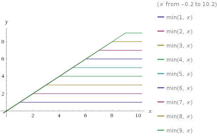
Figure 5. The motions $u_{k}$ described in Section 4.4 when the velocity field $f$ is constant.

We consider a model in which a bunch of people is supposed to move along the real line (say, starting at the origin) with some given velocity $f$, which depends on time. We consider the case in which the environment surrounding the moving people is “tricky”, and some of them risk to get stuck for some time, and they are able to “exit the trap” only by overcoming their past velocity. Concretely, we fix a function $\varphi:[0,+\infty)\to[0,+\infty)$ with

(4.17) $$C_{\varphi}:=\sum_{k=1}^{+\infty}\varphi(k)<+\infty.$$

Then we define

$$p_{k}:=\frac{\varphi(k)}{C_{\varphi}}$$

and we notice that

$$\sum_{k=1}^{+\infty}p_{k}=\frac{1}{C_{\varphi}}\,\sum_{k=1}^{+\infty}\varphi(k)=1.$$

Then, we denote by $u(t)$ the position of the “generic person” at time $t$, with $u(0)=0$. We suppose that some people, say a proportion $p_{1}$ of the total population, move with the prescribed velocity for a unit of time, after which their velocity is the difference between the prescribed velocity at that time and the one at the preceding time with respect to the time unit. In formulas, this says that there is a proportion $p_{1}$ of the total people who travels with velocity

$$\dot{u}_{1}(t):=\left\{\begin{matrix}f(t)&{\mbox{ if }}t\in[0,1],\\ f(t)-f(t-1)&{\mbox{ if }}t>1.\end{matrix}\right.$$

After integrating, we thus obtain that there is a proportion $p_{1}$ of the total people whose position is described by the function

$$u_{1}(t) = \left\{\begin{matrix}\displaystyle\int_{0}^{t}f(\vartheta)\,d\vartheta&{\mbox{ if }}t\in[0,1],\\ \displaystyle\int_{0}^{1}f(\vartheta)\,d\vartheta+\int_{1}^{t}\big{(}f(\vartheta)-f(\vartheta-1)\big{)}\,d\vartheta&{\mbox{ if }}t>1,\end{matrix}\right.$$

$$= \left\{\begin{matrix}\displaystyle\int_{0}^{t}f(\vartheta)\,d\vartheta&{\mbox{ if }}t\in[0,1],\\ \displaystyle\int_{0}^{t}f(\vartheta)\,d\vartheta-\int_{1}^{t}f(\vartheta-1)\,d\vartheta&{\mbox{ if }}t>1,\end{matrix}\right.$$

$$= \left\{\begin{matrix}\displaystyle\int_{0}^{t}f(\vartheta)\,d\vartheta&{\mbox{ if }}t\in[0,1],\\ \displaystyle\int_{0}^{t}f(\vartheta)\,d\vartheta-\int_{0}^{t-1}f(\vartheta)\,d\vartheta&{\mbox{ if }}t>1,\end{matrix}\right.$$

$$= \int_{(t-1)_{+}}^{t}f(\vartheta)\,d\vartheta.$$

For instance, if $f$ is constant, then the position $u_{1}$ grows linearly for a unit of time and then remains put (this would correspond to consider “stopping times” in the motion, see Figure 5).

Similarly, a proportion $p_{2}$ of the total population evolves with prescribed velocity $f$ for two units of time, after which its velocity becomes the difference between the prescribed velocity at that time and the one at the preceding time with respect to two time units, namely

$$\dot{u}_{2}(t):=\left\{\begin{matrix}f(t)&{\mbox{ if }}t\in[0,2],\\ f(t)-f(t-2)&{\mbox{ if }}t>2.\end{matrix}\right.$$

In this case, an integration gives that there is a proportion $p_{2}$ of the total people whose position is described by the function

$$u_{2}(t) = \left\{\begin{matrix}\displaystyle\int_{0}^{t}f(\vartheta)\,d\vartheta&{\mbox{ if }}t\in[0,2],\\ \displaystyle\int_{0}^{2}f(\vartheta)\,d\vartheta+\int_{2}^{t}\big{(}f(\vartheta)-f(\vartheta-2)\big{)}\,d\vartheta&{\mbox{ if }}t>2,\end{matrix}\right.$$

$$= \left\{\begin{matrix}\displaystyle\int_{0}^{t}f(\vartheta)\,d\vartheta&{\mbox{ if }}t\in[0,2],\\ \displaystyle\int_{0}^{t}f(\vartheta)\,d\vartheta-\int_{2}^{t}f(\vartheta-2)\,d\vartheta&{\mbox{ if }}t>2.\end{matrix}\right.$$

$$= \left\{\begin{matrix}\displaystyle\int_{0}^{t}f(\vartheta)\,d\vartheta&{\mbox{ if }}t\in[0,2],\\ \displaystyle\int_{0}^{t}f(\vartheta)\,d\vartheta-\int_{0}^{t-2}f(\vartheta)\,d\vartheta&{\mbox{ if }}t>2.\end{matrix}\right.$$

$$= \int_{(t-2)_{+}}^{t}f(\vartheta)\,d\vartheta.$$

Repeating this argument, we suppose that for each $k\in\mathbb{N}$ we have a proportion $p_{k}$ of the people that move initially with the prescribed velocity $f$, but, after $k$ units of time, get their velocity changed into the difference of the actual velocity field and that of $k$ units of time before (which is indeed a “memory effect”). In this way, we have that a proportion $p_{k}$ of the total population moves with law of motion given by

$$u_{k}(t)=\int_{(t-k)_{+}}^{t}f(\vartheta)\,d\vartheta.$$

The average position of the moving population is then given by

(4.18) $$u(t):=\sum_{k=1}^{+\infty}p_{k}\,u_{k}(t)=\frac{1}{C_{\varphi}}\,\sum_{k=1}^{+\infty}\varphi(k)\,\int_{(t-k)_{+}}^{t}f(\vartheta)\,d\vartheta.$$

We now specialize the computation above for the case

$$\varphi(x):=x^{s-2},$$

with $s\in(0,1)$. Notice that the quantity in (4.17) is finite in this case, and we can denote it simply by $C_{s}$. In addition, we will consider long time asymptotics in $t$ and introduce a small time increment $h$ which is inversely proportional to $t$, namely

$$h:=\frac{1}{t}.$$

In this way, recalling that the motion was supposed to start at the origin (i.e., $u(0)=0$) and using the substitution $\eta:=\vartheta/t$, we can write (4.18) as

(4.19) $$\begin{split}u(t)-u(0)\,&=\frac{1}{C_{s}}\,\sum_{k=1}^{+\infty}k^{s-2}\,\int_{(t-k)_{+}}^{t}f(\vartheta)\,d\vartheta\\ &=\frac{t^{s}\,h}{C_{s}}\,\sum_{k=1}^{+\infty}(hk)^{s-2}\,\int_{(1-kh)_{+}}^{1}f(t\eta)\,d\eta\\ &\simeq\frac{t^{s}}{C_{s}}\,\int_{0}^{+\infty}\left[\lambda^{s-2}\,\int_{(1-\lambda)_{+}}^{1}f(t\eta)\,d\eta\right]\,d\lambda,\end{split}$$

where we have recognized a Riemann sum in the last line.

We also point out that the conditions

$$\lambda\in(0,+\infty)\;{\mbox{ and }}\;0<\xi<\min\{1,\lambda\}$$

are equivalent to

$$0<\xi<1\;{\mbox{ and }}\;\lambda\in(\xi,+\infty),$$

and, furthermore,

$$1-(1-\lambda)_{+}=1-\max\{0,\,1-\lambda\}=\min\{1-0,\,1-(1-\lambda)\}=\min\{1,\lambda\}.$$

Therefore we use the substitution $\xi:=1-\eta$ and we exchange the order of integrations, to deduce from (4.19) that

$$\begin{split}u(t)-u(0)\,&=\frac{t^{s}}{C_{s}}\,\int_{0}^{+\infty}\left[\int_{0}^{\min\{1,\lambda\}}\lambda^{s-2}\,f(t-t\xi)\,d\xi\right]\,d\lambda\\ &=\frac{t^{s}}{C_{s}}\,\int_{0}^{1}\left[\int_{\xi}^{+\infty}\lambda^{s-2}\,f(t-t\xi)\,d\lambda\right]\,d\xi\\ &=\frac{t^{s}}{C_{s}\,(1-s)}\,\int_{0}^{1}\xi^{s-1}\,f(t-t\xi)\,d\xi.\end{split}$$

The substitution $\tau:=t\xi$ then gives

$$u(t)-u(0)=\frac{1}{C_{s}\,(1-s)}\,\int_{0}^{t}\tau^{s-1}\,f(t-\tau)\,d\tau,$$

which, comparing with (2.61) and possibly redefining constants, gives that $\partial^{s}_{C,t}u=f$.

Of course, one can also take into account the case in which the velocity field $f$ is induced by a classical diffusion in space, i.e. $f=\Delta u$, and in this case one obtains the time fractional diffusive equation $\partial^{s}_{C,t}u=\Delta u$.

4.5. Fractional time diffusion arising from heterogeneous media

A very interesting phenomenon to observe is that the geometry of the diffusion medium can naturally transform classical diffusion into an anomalous one. This feature can be very well understood by an elegant model, introduced in [comb] (see also [MR3856678] and the references therein for an exhaustive account of the research in this direction) consisting in random walks on a “comb”, that we briefly reproduce here for the facility of the reader. Given $\varepsilon>0$, the comb may be considered as a transmission medium that is the union of a “backbone” ${\mathcal{B}}:=\mathbb{R}\times\{0\}$ with the “fingers” ${\mathcal{P}}_{k}:=\{\varepsilon k\}\times\mathbb{R}$, namely

$${\mathcal{C}}_{\varepsilon}:={\mathcal{B}}\cup\left(\bigcup_{k\in\mathbb{Z}}{\mathcal{P}}_{k}\right),$$

see Figure 6.

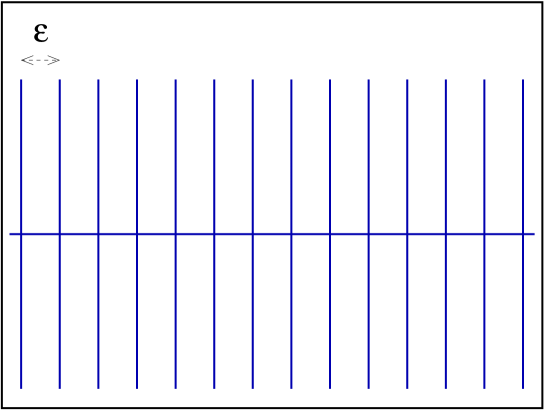
Figure 6. The comb ${\mathcal{C}}_{\varepsilon}$.

We suppose that a particle experiences a random walk on the comb, starting at the origin, with some given horizontal and vertical speeds. In the limit, this random walk can be modeled by the diffusive equation along the comb ${\mathcal{C}}_{\varepsilon}$

(4.20) $$\left\{\begin{matrix}u_{t}=d_{1}\delta_{0}(y)\,u_{xx}+d_{2}\,\varepsilon\,\displaystyle\sum_{k\in\mathbb{Z}}\delta_{0}(\varepsilon k)u_{yy},\\ u(x,y,0)=\delta_{0}(x)\,\delta_{0}(y),\end{matrix}\right.$$

with $d_{1}$, $d_{2}>0$. The case $d_{1}=d_{2}$ corresponds to equal horizontal and vertical speeds of the random walk (and this case is already quite interesting). Also, in the limit as $\varepsilon\searrow 0$, we can consider the Riemann sum approximation

$$\int_{\mathbb{R}}f(y)\,dy\simeq\varepsilon\,\displaystyle\sum_{k\in\mathbb{Z}}f(\varepsilon k),$$

and ${\mathcal{C}}_{\varepsilon}$ tends to cover the whole of $\mathbb{R}^{2}$ when $\varepsilon$ gets small. Accordingly, at least at a formal level, as the fingers of the comb become thicker and thicker, we can think that

$$1=\int_{\mathbb{R}}\delta_{0}(y)\,dy\simeq\varepsilon\,\displaystyle\sum_{k\in\mathbb{Z}}\delta_{0}(\varepsilon k),$$

and reduce (4.20) to the diffusive equation in $\mathbb{R}^{2}$ given by

(4.21) $$\left\{\begin{matrix}u_{t}=d_{1}\delta_{0}(y)\,u_{xx}+d_{2}u_{yy},\\ u(x,y,0)=\delta_{0}(x)\,\delta_{0}(y).\end{matrix}\right.$$

The very interesting feature of (4.21) is that it naturally induces a fractional time diffusion along the backbone. The quantity that experiences this fractional diffusion is the total diffusive mass at a point of the backbone. Namely, one sets

(4.22) $$U(x,t):=\int_{\mathbb{R}}u(x,y,t)\,dy,$$

and we claim that

(4.23) $$\partial^{1/2}_{C,t}\,U(x,t)=\frac{d_{1}}{2\sqrt{d_{2}}}\,\Delta U(x,t)\qquad{\mbox{for all }}\,(x,t)\in\mathbb{R}\times(0,+\infty).$$

Equation (4.23) reveals the very relevant phenomenon that a diffusion governed by the Caputo derivative may naturally arise from classical diffusion, only in view of the particular geometry of the domain.

To check (4.23), we first point out that

(4.24) $$\hat{U}(\xi,0):=\int_{\mathbb{R}}\hat{u}(\xi,y,0)\,dy=\int_{\mathbb{R}}\delta_{0}(y)\,dy=1.$$

Then, we observe that, if $a$, $b\in\mathbb{C}$, and

(4.25) $$\begin{split}&g(y):=b\,e^{-a|y|}\qquad{\mbox{ for any }}y\in\mathbb{R},\\ &{\mbox{then we have that }}\quad g^{\prime\prime}(y)=a^{2}g(y)-2ab\,\delta_{0}(y).\end{split}$$

To check this let $\varphi\in C^{\infty}_{0}(\mathbb{R})$. Then, integrating twice by parts,

$$\frac{1}{b}\,\int_{\mathbb{R}}\big{(}g(y)\varphi^{\prime\prime}(y)-a^{2}g(y)\varphi(y)\big{)}\,dy$$

$$= \int_{0}^{+\infty}e^{-ay}\varphi^{\prime\prime}(y)\,dy+\int_{-\infty}^{0}e^{ay}\varphi^{\prime\prime}(y)\,dy-a^{2}\int_{\mathbb{R}}e^{-a|y|}\varphi(y)\,dy$$

$$= a\int_{0}^{+\infty}e^{-ay}\varphi^{\prime}(y)\,dy-a\int_{-\infty}^{0}e^{ay}\varphi^{\prime}(y)\,dy-a^{2}\int_{\mathbb{R}}e^{-a|y|}\varphi(y)\,dy$$

$$= -2a\varphi(0)+a^{2}\int_{0}^{+\infty}e^{-ay}\varphi(y)\,dy+a^{2}\int_{-\infty}^{0}e^{ay}\varphi^{\prime}(y)\,dy-a^{2}\int_{\mathbb{R}}e^{-a|y|}\varphi(y)\,dy$$

$$= -2a\varphi(0),$$

thus proving (4.25).

We also remark that, in the notation of (4.25), we have that $\delta_{0}(y)g(y)=\delta_{0}(y)g(0)=b\delta_{0}(y)$, and so, for every $c\in\mathbb{R}$,

(4.26) $$g^{\prime\prime}(y)=a^{2}g(y)-b(2a+c)\delta_{0}(y)+c\delta_{0}(y)g(y).$$

Now, taking the Fourier Transform of (4.21) in the variable $x$, using the notation $\hat{u}(\xi,y,t)$ for the Fourier Transform of $u(x,y,t)$, and possibly neglecting normalization constants, we get

(4.27) $$\left\{\begin{matrix}\hat{u}_{t}=-d_{1}|\xi|^{2}\delta_{0}(y)\,\hat{u}+d_{2}\hat{u}_{yy},\\ \hat{u}(\xi,y,0)=\delta_{0}(y).\end{matrix}\right.$$

Now, we take the Laplace Transform of (4.27) in the variable $t$, using the notation $w(\xi,y,\omega)$ for the Laplace Transform of $\hat{u}(\xi,y,t)$, namely $w(\xi,y,\omega):={\mathcal{L}}\hat{u}(\xi,y,\omega)$. In this way, recalling that

$${\mathcal{L}}(\dot{f})=\omega{\mathcal{L}}f(\omega)-f(0),$$

and therefore

$${\mathcal{L}}(\hat{u}_{t})(\xi,y,\omega)=\omega{\mathcal{L}}\hat{u}(\xi,y,\omega)-\hat{u}(\xi,y,0)=\omega w(\xi,y,\omega)-\delta_{0}(y),$$

we deduce from (4.27) that

(4.28) $$\omega w-\delta_{0}(y)=-d_{1}|\xi|^{2}\delta_{0}(y)\,w+d_{2}w_{yy}.$$

That is, setting

$$a(\omega):=\left({\frac{\omega}{d_{2}}}\right)^{1/2},\qquad b(\xi,\omega):=\frac{1}{\left(4d_{2}\omega\right)^{1/2}+d_{1}\,|\xi|^{2}}\qquad{\mbox{and}}\qquad c(\xi):=\frac{d_{1}\,|\xi|^{2}}{d_{2}},$$

we see that

$$b(2a+c)=\frac{2\left(\displaystyle\frac{\omega}{d_{2}}\right)^{1/2}+\displaystyle\frac{d_{1}\,|\xi|^{2}}{d_{2}}}{\left({4d_{2}\omega}\right)^{1/2}+d_{1}\,|\xi|^{2}}=\frac{1}{d_{2}},$$

and hence we can write (4.28) as

$$w_{yy}=\frac{\omega}{d_{2}}\,w-\frac{1}{d_{2}}\delta_{0}(y)+\frac{d_{1}|\xi|^{2}}{d_{2}}\delta_{0}(y)\,w=a^{2}w-b(2a+c)\delta_{0}(y)+c\delta_{0}(y)w.$$

In light of (4.26), we know that this equation is solved by taking $w=g$, that is

$${\mathcal{L}}\hat{u}(\xi,y,\omega)=w(\xi,y,\omega)=b(\xi,\omega)e^{-a(\omega)|y|}.$$

As a consequence, by (4.22),

$${\mathcal{L}}\hat{U}(\xi,t)=\int_{\mathbb{R}}{\mathcal{L}}\hat{u}(\xi,y,\tau)\,dy=\int_{\mathbb{R}}b(\xi,\omega)e^{-a(\omega)|y|}\,dy=\frac{2b(\xi,\omega)}{a}.$$

This and (4.24) give that

$$\left(\left(4d_{2}\omega\right)^{1/2}+d_{1}\,|\xi|^{2}\right){\mathcal{L}}\hat{U}(\xi,t)=\frac{{\mathcal{L}}\hat{U}(\xi,t)}{b(\xi,\omega)}=\frac{2}{a}=\left({\frac{4d_{2}}{\omega}}\right)^{1/2}=2\sqrt{d_{2}}\,{\omega}^{-1/2}\hat{U}(\xi,0),$$

that is

$$\omega^{1/2}{\mathcal{L}}\hat{U}(\xi,t)-{\omega}^{-1/2}\hat{U}(\xi,0)=-\frac{d_{1}}{2\sqrt{d_{2}}}\,|\xi|^{2}\,{\mathcal{L}}\hat{U}(\xi,t).$$

Transforming back and recalling (2.60), we obtain (4.23), as desired.

5. All functions are locally $s$-caloric (up to a small error): proof of (2.12)

We let $(x,t)\in\mathbb{R}\times\mathbb{R}$ and consider the operator $\textswab{L}:=\partial_{t}+(-\Delta)^{s}_{x}$. One defines

$${\mathcal{V}}:=\big{\{}h:\mathbb{R}\times\mathbb{R}\to\mathbb{R}{\mbox{ s.t. $\textswab{L}h=0$ in some neighborhood of the origin in\leavevmode\nobreak\ $\mathbb{R}^{2}$}}\big{\}},$$

and for any $J\in\mathbb{N}$, we define

$${\mathcal{V}}_{J}:=\Big{\{}\big{(}\partial^{\alpha}h(0,0)\big{)}_{{\alpha=(\alpha_{x},\alpha_{t})\in\mathbb{N}\times\mathbb{N}}\atop{\alpha_{x}+\alpha_{t}\in[0,J]}}{\mbox{ with }}h\in{\mathcal{V}}\Big{\}}.$$

Notice that ${\mathcal{V}}_{J}$ is a linear subspace of $\mathbb{R}^{N+1}$, for some $N\in\mathbb{N}$. The core of the proof is to establish the maximal span condition

(5.1) $${\mathcal{V}}_{J}=\mathbb{R}^{N+1}.$$

To this end, we argue for a contradiction and we suppose that ${\mathcal{V}}_{J}$ is a linear subspace strictly smaller than $\mathbb{R}^{N+1}$: hence, there exists

(5.2) $$\nu=(\nu_{0},\dots,\nu_{N})\in S^{N}$$

such that

(5.3) $${\mathcal{V}}_{J}\subseteq\left\{X=(X_{0},\dots,X_{N})\in\mathbb{R}^{J+1}{\mbox{ s.t. }}\nu\cdot X=0\right\}.$$

One considers $\phi$ to be the first eigenfunctions of $(-\Delta)^{s}$ in $(-1,1)$ with Dirichlet data, normalized to have unit norm in $L^{2}(\mathbb{R})$. Accordingly,

$$\left\{\begin{matrix}(-\Delta)^{s}\phi(x)=\lambda\,\phi(x)&{\mbox{ for any }}x\in(-1,1),\cr\phi(x)=0&{\mbox{ for any $x$ outside $(-1,1)$,}}\end{matrix}\right.$$

for some $\lambda>0$.

In view of the boundary properties discussed in Difference 2.6, one can prove that

(5.4) $$\partial^{\ell}\phi(-1+\delta)=\,{\rm const}\,\delta^{s-\ell}(1+o(1)),$$

with $o(1)$ infinitesimal as $\delta\searrow 0$. So, fixed $\varepsilon$, ${\tau}>0$, we define

$$h_{\varepsilon,{\tau}}(x,t):=e^{-{\tau}\,t}\,\phi\left(-1+\varepsilon+\frac{{\tau}^{\frac{1}{2s}}\,x}{\lambda^{\frac{1}{2s}}}\right).$$

This function is smooth for any $x$ in a small neighborhood of the origin and any $t\in\mathbb{R}$, and, in this domain,

$$\textswab{L}h_{\varepsilon,{\tau}}(x,t) = \partial_{t}\left(e^{-{\tau}\,t}\,\phi\left(-1+\varepsilon+\frac{{\tau}^{\frac{1}{2s}}\,x}{\lambda^{\frac{1}{2s}}}\right)\right)+(-\Delta)^{s}_{x}\left(e^{-{\tau}\,t}\,\phi\left(-1+\frac{{\tau}^{\frac{1}{2s}}\,x}{\lambda^{\frac{1}{2s}}}\right)\right)$$

$$= -{\tau}\,e^{-{\tau}\,t}\,\phi\left(-1+\varepsilon+\frac{{\tau}^{\frac{1}{2s}}\,x}{\lambda^{\frac{1}{2s}}}\right)+\frac{{\tau}\,e^{-\tau\,t}}{{\lambda}}(-\Delta)^{s}\phi\left(-1+\varepsilon+\frac{{\tau}^{\frac{1}{2s}}\,x}{\lambda^{\frac{1}{2s}}}\right)$$

$$= -{\tau}\,e^{-{\tau}\,t}\,\phi\left(-1+\varepsilon+\frac{{\tau}^{\frac{1}{2s}}\,x}{\lambda^{\frac{1}{2s}}}\right)+{\tau}\,e^{-{\tau}\,t}\,\phi\left(-1+\varepsilon+\frac{{\tau}^{\frac{1}{2s}}\,x}{\lambda^{\frac{1}{2s}}}\right)$$

$$= 0.$$

This says that $h_{\varepsilon,{\tau}}\in{\mathcal{V}}$ and therefore

$$\big{(}\partial^{\alpha}h_{\varepsilon,{\tau}}0,0)\big{)}_{{\alpha=(\alpha_{x},\alpha_{t})\in\mathbb{N}\times\mathbb{N}}\atop{\alpha_{x}+\alpha_{t}\in[0,J]}}\in{\mathcal{V}}_{J}.$$

This, together with (5.3), implies that, for any fixed and positive $\tau$ and $y$,

$$\begin{split}&0=\sum_{{\alpha=(\alpha_{x},\alpha_{t})\in\mathbb{N}\times\mathbb{N}}\atop{\alpha_{x}+\alpha_{t}\in[0,J]}}\nu_{\alpha}\,\partial^{\alpha}h_{\varepsilon,{\tau}}(0,0)=\sum_{{(\alpha_{x},\alpha_{t})\in\mathbb{N}\times\mathbb{N}}\atop{\alpha_{x}+\alpha_{t}\in[0,J]}}\nu_{(\alpha_{x},\alpha_{t})}\,\partial^{\alpha_{t}}_{t}\partial^{\alpha_{x}}_{x}h_{\varepsilon,{\tau}}(0,0)\\ &\qquad=\left.\sum_{{(\alpha_{x},\alpha_{t})\in\mathbb{N}\times\mathbb{N}}\atop{\alpha_{x}+\alpha_{t}\in[0,J]}}\nu_{(\alpha_{x},\alpha_{t})}(-{\tau})^{\alpha_{t}}\,\left(\frac{{\tau}^{\frac{1}{2s}}}{\lambda^{\frac{1}{2s}}}\right)^{\alpha_{x}}\,e^{-{\tau}\,t}\;\partial^{\alpha_{x}}\phi\left(-1+\varepsilon+\frac{{\tau}^{\frac{1}{2s}}\,x}{\lambda^{\frac{1}{2s}}}\right)\right|_{(x,t)=(0,0)}\\ &\qquad=\sum_{{(\alpha_{x},\alpha_{t})\in\mathbb{N}\times\mathbb{N}}\atop{\alpha_{x}+\alpha_{t}\in[0,J]}}\nu_{(\alpha_{x},\alpha_{t})}\frac{(-1)^{\alpha_{t}}}{\lambda^{\frac{\alpha_{x}}{2s}}}\,{\tau}^{\alpha_{t}+\frac{\alpha_{x}}{2s}}\;\partial^{\alpha_{x}}\phi\left(-1+\varepsilon\right).\end{split}$$

Hence, fixed $\tau>0$, this identity and (5.4) yield that

(5.5) $$0=\sum_{{(\alpha_{x},\alpha_{t})\in\mathbb{N}\times\mathbb{N}}\atop{\alpha_{x}+\alpha_{t}\in[0,J]}}\nu_{(\alpha_{x},\alpha_{t})}\frac{(-1)^{\alpha_{t}}}{\lambda^{\frac{\alpha_{x}}{2s}}}\,{\tau}^{\alpha_{t}+\frac{\alpha_{x}}{2s}}\;\varepsilon^{s-\alpha_{x}}(1+o(1)),$$

with $o(1)$ infinitesimal as $\varepsilon\searrow 0$.

We now take $\bar{\alpha}_{x}$ be the largest integer $\alpha_{x}$ for which there exists an integer $\alpha_{t}$ such that $\bar{\alpha}_{x}+\alpha_{t}\in[0,J]$ and $\nu_{(\bar{\alpha}_{x},\alpha_{t})}\neq 0$. Notice that this definition is well-posed, since not all the $\nu_{(\alpha_{x},\alpha_{t})}$ can vanish, due to (5.2). Then, (5.5) becomes

(5.6) $$0=\sum_{{{(\alpha_{x},\alpha_{t})\in\mathbb{N}\times\mathbb{N}}\atop{\alpha_{x}+\alpha_{t}\in[0,J]}}\atop{\alpha_{x}\leqslant\bar{\alpha}_{x}}}\nu_{(\alpha_{x},\alpha_{t})}\frac{(-1)^{\alpha_{t}}}{\lambda^{\frac{\alpha_{x}}{2s}}}\,{\tau}^{\alpha_{t}+\frac{\alpha_{x}}{2s}}\;\varepsilon^{s-\alpha_{x}}(1+o(1)),$$

since the other coefficients vanish by definition of $\bar{\alpha}_{x}$.

Thus, we multiply (5.6) by $\varepsilon^{\bar{\alpha}_{x}-s}{\tau}^{-\frac{\bar{\alpha}_{x}}{2s}}$ and we take the limit as $\varepsilon\searrow 0$: in this way, we obtain that

$$0 = \lim_{\varepsilon\searrow 0}\sum_{{{(\alpha_{x},\alpha_{t})\in\mathbb{N}\times\mathbb{N}}\atop{\alpha_{x}+\alpha_{t}\in[0,J]}}\atop{\alpha_{x}\leqslant\bar{\alpha}_{x}}}\nu_{(\alpha_{x},\alpha_{t})}\frac{(-1)^{\alpha_{t}}}{\lambda^{\frac{\alpha_{x}}{2s}}}\,{\tau}^{\alpha_{t}+\frac{\alpha_{x}}{2s}-\frac{\bar{\alpha}_{x}}{2s}}\;\varepsilon^{\bar{\alpha}_{x}-\alpha_{x}}(1+o(1))$$

$$= \sum_{{{\alpha_{t}\in\mathbb{N}}\atop{\bar{\alpha}_{x}+\alpha_{t}\in[0,J]}}}\nu_{(\bar{\alpha}_{x},\alpha_{t})}\frac{(-1)^{\alpha_{t}}}{\lambda^{\frac{\bar{\alpha}_{x}}{2s}}}\,{\tau}^{\alpha_{t}}.$$

Since this is valid for any $\tau>0$, by the Identity Principle for Polynomials we obtain that

$$\nu_{(\bar{\alpha}_{x},\alpha_{t})}\frac{(-1)^{\alpha_{t}}}{\lambda^{\frac{\bar{\alpha}_{x}}{2s}}}=0,$$

and thus $\nu_{(\bar{\alpha}_{x},\alpha_{t})}=0$, for any integer $\alpha_{t}$ for which $\bar{\alpha}_{x}+\alpha_{t}\in[0,J]$. But this is in contradiction with the definition of $\bar{\alpha}_{x}$ and so we have completed the proof of (5.1).

From this maximal span property, the proof of (2.12) follows by scaling (arguing as done, for instance, in [HB]).

$\langle\langle$The longest appendix measured 26cm (10.24in) when it was removed from 72-year-old Safranco August (Croatia) during an autopsy at the Ljudevit Jurak University Department of Pathology, Zagreb, Croatia, on 26 August 2006.$\rangle\rangle$

(Source: http://www.guinnessworldrecords.com/world-records/largest-appendix-removed)

Appendix A Confirmation of (2.7)

We write $\Delta_{x}$ to denote the Laplacian in the coordinates $x\in\mathbb{R}^{n}$. In this way, the total Laplacian in the variables $(x,y)\in\mathbb{R}^{n}\times(0,+\infty)$ can be written as

(A.1) $$\Delta=\Delta_{x}+\partial^{2}_{y}.$$

Given a (smooth and bounded, in the light of footnote 3 on page 3) $u:\mathbb{R}^{n}\to\mathbb{R}$, we take $U:=E_{u}$ be (smooth and bounded) as in (2.6).

We also consider the operator

(A.2) $$Lu(x):=-\partial_{y}E_{u}(x,0)$$

and we take $V(x,y):=-\partial_{y}U(x,y)$. Notice that $\Delta V=-\partial_{y}\Delta U=0$ in $\mathbb{R}^{n}\times(0,+\infty)$ and $V(x,0)=Lu(x)$ for any $x\in\mathbb{R}^{n}$. In this sense, $V$ is the harmonic extension of $Lu$ and so we can write $V=E_{Lu}$ and so, in the notation of (A.2), and recalling (2.6) and (A.1), we have

$$L(Lu)(x)=-\partial_{y}E_{Lu}(x,0)=-\partial_{y}V(x,0)=\partial_{y}^{2}U(x,0)$$

$$\qquad=\Delta U(x,0)-\Delta_{x}U(x,0)=-\Delta_{x}U(x,0)=-\Delta u(x).$$

This gives that $L^{2}=-\Delta$, which is consistent with $L=(-\Delta)^{1/2}$, thanks to (2.5).

Appendix B Proof of (2.10)

Let $u\in{\mathcal{S}}$. By (2.9), we can write

(B.1) $$\sup_{x\in\mathbb{R}^{n}}(1+|x|^{n})\left|u(x)\right|+\sup_{x\in\mathbb{R}^{n}}(1+|x|^{n+2})\left|D^{2}u(x)\right|\leqslant\,{\rm const}\,.$$

Fixed $x\in\mathbb{R}^{n}$ (with $|x|$ to be taken large), recalling the notation in (2.3), we consider the map $y\mapsto\delta_{u}(x,y)$ and we observe that

$$\delta_{u}(x,0)=0,$$

$$\nabla_{y}\delta_{u}(x,y)=\nabla u(x+y)-\nabla u(x-y),$$

and $$D^{2}_{y}\delta_{u}(x,y)=D^{2}u(x+y)+D^{2}u(x-y).$$

Hence, if $|Y|\leqslant|x|/2$ we have that $|x\pm Y|\geqslant|x|-|Y|\geqslant|x|/2$, and thus

$$\big{|}D^{2}_{y}\delta_{u}(x,Y)\big{|}\leqslant 2\sup_{|\zeta|\geqslant|x|/2}\big{|}D^{2}u(\zeta)\big{|}\leqslant 2\sup_{|\zeta|\geqslant|x|/2}\frac{(2|\zeta|)^{n+2}\big{|}D^{2}u(\zeta)\big{|}}{|x|^{n+2}}\leqslant\frac{\,{\rm const}\,}{|x|^{n+2}},$$

thanks to (B.1).

Therefore, a second order Taylor expansion of $\delta_{u}$ in the variable $y$ gives that, if $|y|\leqslant|x|/2$,

$$\big{|}\delta_{u}(x,y)\big{|}\leqslant\sup_{|Y|\leqslant|x|/2}\left|\delta_{u}(x,0)+\nabla\delta_{u}(x,0)\cdot y+\frac{D^{2}\delta_{u}(x,Y)\,y\cdot y}{2}\right|$$

$$\qquad=\sup_{|Y|\leqslant|x|/2}\left|\frac{D^{2}\delta_{u}(x,Y)\,y\cdot y}{2}\right|\leqslant\frac{\,{\rm const}\,\,|y|^{2}}{|x|^{n+2}}.$$

Consequently,

(B.2) $$\left|\int_{B_{|x|/2}}\frac{\delta_{u}(x,y)}{|y|^{n+2s}}\,dy\right|\leqslant\frac{\,{\rm const}\,}{|x|^{n+2}}\int_{B_{|x|/2}}\frac{|y|^{2}}{|y|^{n+2s}}\,dy\leqslant\frac{\,{\rm const}\,\,|x|^{2-2s}}{|x|^{n+2}}=\frac{\,{\rm const}\,}{|x|^{n+2s}}.$$

Moreover, by (B.1),

$$\left|\int_{\mathbb{R}^{n}\setminus B_{|x|/2}}\frac{\delta_{u}(x,y)}{|y|^{n+2s}}\,dy\right|$$

$$\leqslant \int_{\mathbb{R}^{n}\setminus B_{|x|/2}}\frac{|u(x+y)|}{|y|^{n+2s}}\,dy+\int_{\mathbb{R}^{n}\setminus B_{|x|/2}}\frac{|u(x-y)|}{|y|^{n+2s}}\,dy+2\int_{\mathbb{R}^{n}\setminus B_{|x|/2}}\frac{|u(x)|}{|y|^{n+2s}}\,dy$$

$$\leqslant \int_{\mathbb{R}^{n}\setminus B_{|x|/2}}\frac{|u(x+y)|}{(|x|/2)^{n+2s}}\,dy+\int_{\mathbb{R}^{n}\setminus B_{|x|/2}}\frac{|u(x-y)|}{(|x|/2)^{n+2s}}\,dy+\frac{\,{\rm const}\,\,|u(x)|}{|x|^{2s}}$$

$$\leqslant \frac{\,{\rm const}\,}{|x|^{n+2s}}\int_{\mathbb{R}^{n}}|u(\zeta)|\,d\zeta+\frac{\,{\rm const}\,\,|u(x)|}{|x|^{2s}}$$

$$\leqslant \frac{\,{\rm const}\,}{|x|^{n+2s}}.$$

This and (B.2), recalling (2.3), establish (2.10).

Appendix C Proof of (2.14)

Let $M:=\frac{1}{2n}\,\left(1+\sup_{B_{1}}|f|\right)$ and $v(x):=M(1-|x|^{2})-u(x)$. Notice that $v=0$ along $\partial B_{1}$ and

$$\Delta v=-2nM-\Delta u\leqslant-M-f\leqslant-M+\sup_{B_{1}}|f|\leqslant 0$$

in $B_{1}$. Consequently, $v\geqslant 0$ in $B_{1}$, which gives that $u(x)\leqslant M(1-|x|^{2})$.

Arguing similarly, by looking at $\tilde{v}(x):=M(1-|x|^{2})+u(x)$, one sees that $-u(x)\leqslant M(1-|x|^{2})$. Accordingly, we have that

$$|u(x)|\leqslant M(1-|x|^{2})\leqslant M(1+|x|)(1-|x|)\leqslant 2M(1-|x|).$$

This proves (2.14).

Appendix D Proof of (2.17)

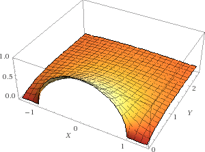
Figure 7. Harmonic extension in the halfplane of the function $\mathbb{R}\ni x\mapsto(1-x^{2})_{+}^{1/2}$.

The idea of the proof is described in Figure 7. The trace of the function in Figure 7 is exactly the function $u_{1/2}$ in (2.16). The function plotted in Figure 7 is the harmonic extension of $u_{1/2}$ in the halfplane (like an elastic membrane pinned at the halfcircumference along the trace). Our objective is to show that the normal derivative of such extended function along the trace is constant, and so we can make use of the extension method in (2.6) and (2.7) to obtain (2.17).

In further detail, we use complex coordinates, identifying $(x,y)\in\mathbb{R}\times(0,+\infty)$ with $z:=x+iy\in\mathbb{C}$ with $\Im(z)>0$. Also, as customary, we define the principal square root in the cut complex plane

$$\mathbb{C}_{\star}:=\{z=re^{{i\varphi}}{\text{ with }}r>0{\mbox{ and }}-\pi<\varphi<\pi\}$$

by defining, for any $z=re^{{i\varphi}}\in\mathbb{C}_{\star}$,

(D.1) $${\surd}({z}):=\sqrt{r}\,e^{i\varphi/2},$$

see Figure 8 (for typographical convenience, we distinguish between the complex and the real square root, by using the symbols ${\displaystyle{\surd}}(\cdot)$ and $\sqrt{\cdot}$ respectively).

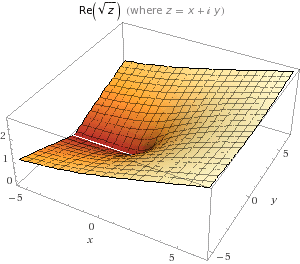
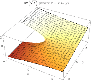
Figure 8. Real and imaginary part of the complex principal square root.

The principal square root function is defined using the nonpositive real axis as a “branch cut” and

(D.2) $$\big{(}\displaystyle{\surd}({z})\big{)}^{2}=r\,e^{i\varphi}=z.$$

Moreover,

(D.3) the function $${\surd} \mathbb{C}_{\star}$$ is holomorphic in 

(D.4) $${\mbox{and }}\;\partial_{z}\displaystyle{\surd}({z})=\frac{1}{2\displaystyle{\surd}(z)}.$$

To check these facts, we take $z\in\mathbb{C}_{\star}$: since $\mathbb{C}_{\star}$ is open, we have that $z+w\in\mathbb{C}_{\star}$ for any $w\in\mathbb{C}\setminus\{0\}$ with small module. Consequently, by (D.2), we obtain that

$$w=(z+w)-z=\big{(}\displaystyle{\surd}({z+w})\big{)}^{2}-\big{(}\displaystyle{\surd}({z})\big{)}^{2}$$

$$\qquad=\Big{(}\displaystyle{\surd}({z+w})+\displaystyle{\surd}({z})\Big{)}\Big{(}\displaystyle{\surd}({z+w})-\displaystyle{\surd}({z})\Big{)}.$$

Dividing by $w$ and taking the limit, we thus find that

(D.5) $$\begin{split}1\;&=\lim_{w\to 0}\Big{(}\displaystyle{\surd}({z+w})+\displaystyle{\surd}({z})\Big{)}\,\frac{\displaystyle{\surd}({z+w})-\displaystyle{\surd}({z})}{w}\\ &=2\displaystyle{\surd}({z})\;\lim_{w\to 0}\frac{\displaystyle{\surd}({z+w})-\displaystyle{\surd}({z})}{w}\end{split}$$

Since $\mathbb{C}_{\star}\subseteq\mathbb{C}\setminus\{0\}$, we have that $z\neq 0$, and thus $\displaystyle{\surd}(z)\neq 0$. As a result, we can divide (D.5) by $2\displaystyle{\surd}({z})$ and conclude that

$$\lim_{w\to 0}\frac{\displaystyle{\surd}({z+w})-\displaystyle{\surd}({z})}{w}=\frac{1}{2\displaystyle{\surd}({z})},$$

which establishes, at the same time, both (D.3) and (D.4), as desired.

We also remark that

(D.6) if $$z\in\mathbb{C} \Im(z)>0 1-z^{2}\in\mathbb{C}_{\star}$$ with , then .

To check this, if $z=x+iy$ with $y>0$, we observe that

(D.7) $$1-z^{2}=1-(x+iy)^{2}=1-x^{2}+y^{2}-2ixy.$$

Hence, if $1-z^{2}$ lies on the real axis, we have that $xy=0$, and so $x=0$. Then, the real part of $1-z^{2}$ in this case is equal to $1+y^{2}$ which is strictly positive. This proves (D.6).

Thanks to (D.6), for any $z\in\mathbb{C}$ with $\Im(z)>0$ we can define the function $\displaystyle{\surd}(1-z^{2})$. From (D.7), we can write

$$\begin{split}&1-z^{2}=r(x,y)\,e^{{i\varphi(x,y)}},\\ {\mbox{where }}\;&r(x,y)=\big{(}(1-x^{2}+y^{2})^{2}+4x^{2}y^{2}\big{)}^{1/2},\\ &r(x,y)\,\cos\varphi(x,y)=1-x^{2}+y^{2}\\ {\mbox{and }}&r(x,y)\,\sin\varphi(x,y)=2xy.\end{split}$$

Notice that

$$\lim_{y\searrow 0}r(x,y)=\big{(}(1-x^{2})^{2}\big{)}^{1/2}=|1-x^{2}|.$$

As a consequence,

$$|1-x^{2}|\,\lim_{y\searrow 0}\cos\varphi(x,y)=\lim_{y\searrow 0}r(x,y)\,\cos\varphi(x,y)=\lim_{y\searrow 0}(1-x^{2}+y^{2})=1-x^{2}$$

and $$|1-x^{2}|\,\lim_{y\searrow 0}\sin\varphi(x,y)=\lim_{y\searrow 0}r(x,y)\,\sin\varphi(x,y)=\lim_{y\searrow 0}2xy=0.$$

This says that, if $x^{2}>1$ then

$$\lim_{y\searrow 0}\cos\varphi(x,y)=-1$$

and $$\lim_{y\searrow 0}\sin\varphi(x,y)=0,$$

while if $x^{2}<1$ then

$$\lim_{y\searrow 0}\cos\varphi(x,y)=1$$

and $$\lim_{y\searrow 0}\sin\varphi(x,y)=0.$$

On this account, we deduce that

(D.8) $$\lim_{y\searrow 0}\varphi(x,y)=\left\{\begin{matrix}\pi&{\mbox{ if }}x^{2}>1,\\ 0&{\mbox{ if }}x^{2}<1\end{matrix}\right.$$

and therefore, recalling (D.1),

(D.9) $$\begin{split}&\lim_{y\searrow 0}\displaystyle{\surd}(1-z^{2})=\lim_{y\searrow 0}\sqrt{r(x,y)}\,e^{i\varphi(x,y)/2}=\left\{\begin{matrix}\sqrt{|1-x^{2}|}\;e^{i\pi/2}&{\mbox{ if }}x^{2}>1,\\ \sqrt{|1-x^{2}|}\;e^{i0}&{\mbox{ if }}x^{2}<1,\\ 0&{\mbox{ if }}x^{2}=1\end{matrix}\right.\\ &\qquad\qquad=\left\{\begin{matrix}i\,\sqrt{|1-x^{2}|}&{\mbox{ if }}x^{2}>1,\\ \sqrt{|1-x^{2}|}&{\mbox{ if }}x^{2}<1,\\ 0&{\mbox{ if }}x^{2}=1.\end{matrix}\right.\end{split}$$

This implies that

(D.10) $$\begin{split}\lim_{y\searrow 0}\Re\Big{(}\displaystyle{\surd}(1-z^{2})\Big{)}\;&=\left\{\begin{matrix}0&{\mbox{ if }}x^{2}\geqslant 1,\\ \sqrt{|1-x^{2}|}&{\mbox{ if }}x^{2}<1\end{matrix}\right.\\ &=(1-x^{2})^{1/2}_{+}.\end{split}$$

Now we define

$$z=x+iy\mapsto\Re\Big{(}\displaystyle{\surd}(1-z^{2})+iz\Big{)}=:U_{1/2}(x,y).$$

The function $U_{1/2}$ is the harmonic extension of $u_{1/2}$ in the halfplane, as plotted in Figure 7. Indeed, from (D.10),

$$\lim_{y\searrow 0}U_{1/2}(x,y)=\lim_{y\searrow 0}\Re\Big{(}\displaystyle{\surd}(1-z^{2})+ix-y\Big{)}=(1-x^{2})^{1/2}_{+}=u_{1/2}(x).$$

Furthermore, from (D.3), we have that $U_{1/2}$ is the real part of a holomorphic function in the halfplane and so it is harmonic.

These considerations give that $U_{1/2}$ solves the harmonic extension problem in (2.6), hence, in the light of (2.7),

(D.11) $$\begin{split}&(-\Delta)^{1/2}u_{1/2}(x)=\lim_{y\searrow 0}-\partial_{y}U_{1/2}(x,y)=\lim_{y\searrow 0}-\Re\Big{(}\partial_{y}\displaystyle{\surd}(1-z^{2})+i\partial_{y}z\Big{)}\\ &\qquad\qquad=\lim_{y\searrow 0}-\Re\Big{(}\partial_{y}\displaystyle{\surd}(1-z^{2})-1\Big{)}=1-\lim_{y\searrow 0}\Re\Big{(}\partial_{y}\displaystyle{\surd}(1-z^{2})\Big{)}.\end{split}$$

Now, recalling (D.4), we see that, for any $x\in(-1,1)$ and small $y>0$,

(D.12) $$\partial_{y}\displaystyle{\surd}(1-z^{2})=\partial_{z}\displaystyle{\surd}(1-z^{2})\;\partial_{y}z=\frac{1}{2\displaystyle{\surd}(1-z^{2})}\;\partial_{z}(1-z^{2})\;\partial_{y}(x+iy)=-\frac{iz}{\displaystyle{\surd}(1-z^{2})}.$$

We stress that the latter denominator does not vanish when $x\in(-1,1)$ and $y>0$ is small. So, using that $\Re(ZW)=\Re Z\Re W-\Im Z\Im W$ for any $Z$, $W\in\mathbb{C}$, we obtain that

(D.13) $$\begin{split}&y=\Re\big{(}-i(x+iy)\big{)}=\Re(-iz)=\Re\Big{(}\displaystyle{\surd}(1-z^{2})\;\partial_{y}\displaystyle{\surd}(1-z^{2})\Big{)}\\ &\qquad=\Re\Big{(}\displaystyle{\surd}(1-z^{2})\Big{)}\;\Re\Big{(}\partial_{y}\displaystyle{\surd}(1-z^{2})\Big{)}-\Im\Big{(}\displaystyle{\surd}(1-z^{2})\Big{)}\;\Im\Big{(}\partial_{y}\displaystyle{\surd}(1-z^{2})\Big{)}.\end{split}$$

From (D.9), for any $x\in(-1,1)$ we have that

$$\lim_{y\searrow 0}\Im\Big{(}\displaystyle{\surd}(1-z^{2})\Big{)}=\Im\Big{(}\sqrt{|1-x^{2}|}\Big{)}=0.$$

This and the fact that $\partial_{y}\displaystyle{\surd}(1-z^{2})$ is bounded (in view of (D.12)) give that, for any $x\in(-1,1)$,

$$\lim_{y\searrow 0}\Im\Big{(}\displaystyle{\surd}(1-z^{2})\Big{)}\;\Im\Big{(}\partial_{y}\displaystyle{\surd}(1-z^{2})\Big{)}=0.$$

This, (D.9) and (D.13) imply that, for any $x\in(-1,1)$,

$$0=\lim_{y\searrow 0}y=\lim_{y\searrow 0}\Re\Big{(}\displaystyle{\surd}(1-z^{2})\Big{)}\;\Re\Big{(}\partial_{y}\displaystyle{\surd}(1-z^{2})\Big{)}-\Im\Big{(}\displaystyle{\surd}(1-z^{2})\Big{)}\;\Im\Big{(}\partial_{y}\displaystyle{\surd}(1-z^{2})\Big{)}$$

$$\qquad=\Re\Big{(}\sqrt{|1-x^{2}|}\Big{)}\;\lim_{y\searrow 0}\Re\Big{(}\partial_{y}\displaystyle{\surd}(1-z^{2})\Big{)}+0$$

$$\qquad=\sqrt{|1-x^{2}|}\;\lim_{y\searrow 0}\Re\Big{(}\partial_{y}\displaystyle{\surd}(1-z^{2})\Big{)}$$

and therefore

(D.14) $$\lim_{y\searrow 0}\Re\Big{(}\partial_{y}\displaystyle{\surd}(1-z^{2})\Big{)}=0.$$

Plugging this information into (D.11), we conclude the proof of (2.17), as desired.

Appendix E Deducing (2.19) from (2.15) using a space inversion

From (2.15), up to a translation, we know that

(E.1) the function $$\mathbb{R}\ni x\mapsto v_{s}(x):=(x-1)_{+}^{s} s (1,+\infty)$$ is -harmonic in .

We let $w_{s}$ be the space inversion of $v_{s}$ induced by the Kelvin transform in the fractional setting, namely

$$w_{s}(x):=|x|^{2s-1}\,v_{s}\left(\frac{x}{|x|^{2}}\right)=|x|^{2s-1}\,\left(\frac{x}{|x|^{2}}-1\right)_{+}^{s}=\left\{\begin{matrix}x^{s-1}(1-x)^{s}&{\mbox{ if }}x\in(0,1),\\ 0&{\mbox{ otherwise}}.\end{matrix}\right..$$

By (E.1), see Corollary 2.3 in [MR2964681], it follows that $w_{s}(x)$ is $s$-harmonic in $(0,1)$. Consequently, the function

$$w^{\star}_{s}(x):=w_{s}(1-x)=\left\{\begin{matrix}x^{s}(1-x)^{s-1}&{\mbox{ if }}x\in(0,1),\\ 0&{\mbox{ otherwise}}.\end{matrix}\right.$$

is also $s$-harmonic in $(0,1)$. We thereby conclude that the function

$$W^{\star}_{s}(x):=w_{s}(x)-w^{\star}_{s}(x)=\left\{\begin{matrix}x^{s-1}(1-x)^{s}-x^{s}(1-x)^{s-1}&{\mbox{ if }}x\in(0,1),\\ 0&{\mbox{ otherwise}}.\end{matrix}\right.$$

is also $s$-harmonic in $(0,1)$. See Figure 9 for a picture of $w_{s}$ and $W^{\star}_{s}$ when $s=1/2$. Let now

$$U_{s}(x):=x_{+}^{s}(1-x)_{+}^{s}=\left\{\begin{matrix}x^{s}(1-x)^{s}&{\mbox{ if }}x\in(0,1),\\ 0&{\mbox{ otherwise}}.\end{matrix}\right.$$

and notice that $U_{s}$ is the primitive of $sW^{\star}_{s}$. Since the latter function is $s$-harmonic in $(0,1)$, after an integration we thereby deduce that $(-\Delta)^{s}U_{s}=\,{\rm const}\,$ in $(0,1)$. This and the fact that

$$U_{s}\left(\frac{x+1}{2}\right)=2^{-s}\,u_{s}(x)$$

imply (2.19).

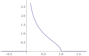
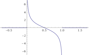
Figure 9. The functions $w_{1/2}$ and $W^{\star}_{1/2}$.

Appendix F Proof of (2.21)

Fixed $y\in\mathbb{R}^{n}\setminus\{0\}$ we let ${\mathcal{R}}^{y}$ be a rotation which sends $\frac{y}{|y|}$ into the vector $e_{1}=(1,0,\dots,0)$, that is

(F.1) $$\sum_{k=1}^{n}{\mathcal{R}}_{ik}^{y}\,y_{k}=|y|\delta_{i1},$$

for any $i\in\{1,\dots,n\}$. We also denote by

$$K(y):=\frac{y}{|y|^{2}}$$

the so-called Kelvin Transform. We recall that for any $i$, $j\in\{1,\dots,n\}$,

$$\partial_{y_{i}}K_{j}(y)=\frac{\delta_{ij}}{|y|^{2}}-\frac{2y_{i}y_{j}}{|y|^{4}}$$

and so, by (F.1),

$$\Big{(}{\mathcal{R}}^{y}\;(DK(y))\;({\mathcal{R}}^{y})^{-1}\Big{)}_{ij}=\sum_{k,h=1}^{n}{\mathcal{R}}^{y}_{ik}\,\partial_{y_{k}}K_{h}(y)\,{\mathcal{R}}^{y}_{jh}=\frac{\delta_{ij}}{|y|^{2}}-\frac{2\delta_{i1}\delta_{j1}}{|y|^{2}}.$$

This says that ${\mathcal{R}}^{y}\;(DK(y))\;({\mathcal{R}}^{y})^{-1}$ is a diagonal matrix, with first entry equal to $-\frac{1}{|y|^{2}}$ and the others equal to $\frac{1}{|y|^{2}}$.

As a result,

(F.2) $$\big{|}\det(DK(y))\big{|}=\Big{|}\det\big{(}{\mathcal{R}}^{y}\;(DK(y))\;({\mathcal{R}}^{y})^{-1}\big{)}\Big{|}=\frac{1}{|y|^{2n}}.$$

The Kelvin Transform is also useful to write the Green function of the ball $B_{1}$, see e.g. formula (41) on p. 40 and Theorem 13 on p. 35 of [MR1625845]. Namely, we take $n\geqslant 3$ for simplicity, and we write

$$G(x,y):=\,{\rm const}\,\left(\frac{1}{|y-x|^{n-2}}-\frac{1}{\big{|}\,|x|(y-K(x))\big{|}^{n-2}}\right)$$

$$\qquad\qquad=\,{\rm const}\,\left(\frac{1}{|x-y|^{n-2}}-\frac{1}{\big{|}\,|y|(x-K(y))\big{|}^{n-2}}\right)=G(y,x)$$

and, for a suitable choice of the constant, for any $x\in B_{1}$ we can write the solution of (2.20) in the form

$$u(x)=\int_{B_{1}}f(y)\,G(x,y)\,dy.$$

see e.g. page 35 in [MR1625845].

On this account, we have that, for any $x\in B_{1}$,

$$|\nabla u(x)| \leqslant \int_{B_{1}}|f(y)|\,|\partial_{x}G(x,y)|\,dy$$

$$\leqslant \,{\rm const}\,\sup_{B_{1}}|f|\int_{B_{1}}\left(\frac{1}{|x-y|^{n-1}}+\frac{1}{|y|^{n-2}\big{|}x-K(y)\big{|}^{n-1}}\right)\,dy$$

$$\leqslant \,{\rm const}\,\sup_{B_{1}}|f|\left(\int_{B_{2}}\frac{d\zeta}{|\zeta|^{n-1}}+\int_{\mathbb{R}^{n}\setminus B_{1}}\frac{d\eta}{|\eta|^{n+2}\big{|}x-\eta\big{|}^{n-1}}\right)$$

$$\leqslant \,{\rm const}\,\sup_{B_{1}}|f|\left(1+\int_{B_{2}\setminus B_{1}}\frac{d\eta}{|x-\eta|^{n-1}}+\int_{\mathbb{R}^{n}\setminus B_{2}}\frac{d\eta}{|\eta|^{n+2}}\right)$$

$$\leqslant \,{\rm const}\,\sup_{B_{1}}|f|.$$

Notice that here we have used the transformations $\zeta:=x-y$ and $\eta:=K(y)$, exploiting also (F.2). The claim in (2.21) is thus established.

Appendix G Proof of (2.24) and probabilistic insights

We give a proof of (2.24) by taking a derivative of (2.17). To this aim, we claim that

(G.1) $$\begin{split}&\frac{d}{dx}\int_{\mathbb{R}}\frac{u_{1/2}(x+y)+u_{1/2}(x-y)-2u_{1/2}(x)}{|y|^{2}}\,dy\\ =\;&-\int_{\mathbb{R}}\frac{(x+y)u_{-1/2}(x+y)+(x-y)u_{-1/2}(x-y)-2xu_{-1/2}(x)}{|y|^{2}}\,dy.\end{split}$$

To this end, we fix $x\in(-1,1)$ and $h\in\mathbb{R}$. We define

$$\ell_{x}:=\min\{|x-1|,\,|x+1|\}>0.$$

In the sequel, we will take $|h|$ as small as we wish in order to compute incremental quotients, hence we can assume that

(G.2) $$|h|<\frac{\ell_{x}}{4}.$$

We also define

(G.3) $$I_{x}(h):=\Big{\{}y\in\mathbb{R}{\mbox{ s.t. }}\min\{|(x+y)-1|,\,|(x-y)-1|,\,|(x+y)+1|,\,|(x-y)+1|\}\leqslant 2|h|\Big{\}}.$$

Since $I_{x}(h)\subseteq(x-1-2|h|,x-1+2|h|)\cup(x+1-2|h|,x+1+2|h|)\cup(1-x-2|h|,1-x+2|h|)\cup(-1-x-2|h|,-1-x+2|h|)$, we have that

(G.4) the measure of $$I_{x} \,{\rm const}\,|h|$$ is less than .

Furthermore,

(G.5) $$I_{x}(h)\subseteq\left\{y\in\mathbb{R}{\mbox{ s.t. }}|y|\geqslant\frac{\ell_{x}}{2}\right\}.$$

To check this, let $y\in I_{x}(h)$. Then, by (G.3), there exist $\sigma_{1,x,y}$, $\sigma_{2,x,y}\in\{-1,1\}$ such that

$$|x+\sigma_{1,x,y}y+\sigma_{2,x,y}|\leqslant 2|h|$$

and therefore

$$|y|=|\sigma_{1,x,y}y|\geqslant|x+\sigma_{2,x,y}|-|x+\sigma_{1,x,y}y+\sigma_{2,x,y}|\geqslant\ell_{x}-2|h|\geqslant\frac{\ell_{x}}{2},$$

where the last inequality is a consequence of (G.2), and this establishes (G.5).

Now, we introduce the following notation for the incremental quotient

$$Q_{h}(x,y):=\frac{\big{(}u_{1/2}(x+y+h)+u_{1/2}(x-y+h)-2u_{1/2}(x+h)\big{)}-\big{(}u_{1/2}(x+y)+u_{1/2}(x-y)-2u_{1/2}(x)\big{)}}{h}$$

and we observe that, since $u_{1/2}$ is globally Hölder continuous with exponent $1/2$, it holds that

$$\begin{split}|Q_{h}(x,y)|\;&\leqslant\frac{\big{|}u_{1/2}(x+y+h)-u_{1/2}(x+y)\big{|}+\big{|}u_{1/2}(x-y+h)-u_{1/2}(x-y)\big{|}+2\,\big{|}u_{1/2}(x+h)-u_{1/2}(x)\big{|}}{|h|}\\ &\leqslant\frac{\,{\rm const}\,|h|^{1/2}}{|h|}\\ &=\frac{\,{\rm const}\,}{|h|^{1/2}},\end{split}$$

for any $x$, $y\in\mathbb{R}$. Consequently, recalling (G.4) and (G.5), we conclude that

(G.6) $$\lim_{h\to 0}\left|\int_{I_{x}(h)}\frac{Q_{h}(x,y)}{|y|^{2}}\,dy\right|\leqslant\lim_{h\to 0}\int_{I_{x}(h)}\frac{\,{\rm const}\,}{|h|^{1/2}\,\ell_{x}^{2}}\,dy\leqslant\lim_{h\to 0}\frac{\,{\rm const}\,|h|}{|h|^{1/2}\,\ell_{x}^{2}}=0.$$

Now we take derivatives of $u_{1/2}$. For this, we observe that, for any $\xi\in(-1,1)$,

$$u_{1/2}^{\prime}(\xi)=-\xi(1-\xi^{2})^{-1/2}=-\xi u_{-1/2}(\xi).$$

Since the values outside $(-1,1)$ are trivial, this implies that

(G.7) $$u_{1/2}^{\prime}(\xi)=-\xi u_{-1/2}(\xi)\quad{\mbox{ for any }}\xi\in\mathbb{R}\setminus\{-1,1\}.$$

Now, by (G.3), we know that if $y\in\mathbb{R}\setminus I_{x}(h)$ we have that $x+y+t\in\mathbb{R}\setminus\{-1,1\}$ for all $t\in\mathbb{R}$ with $|t|<|h|$ and therefore we can exploit (G.7) and find that

$$\lim_{h\to 0}\frac{u_{1/2}(x+y+h)-u_{1/2}(x+y)}{h}=-(x+y)u_{-1/2}(x+y).$$

Similar arguments show that, for any $y\in\mathbb{R}\setminus I_{x}(h)$,

$$\lim_{h\to 0}\frac{u_{1/2}(x-y+h)-u_{1/2}(x-y)}{h}=-(x-y)u_{-1/2}(x-y)$$

and $$\lim_{h\to 0}\frac{u_{1/2}(x+h)-u_{1/2}(x)}{h}=-xu_{-1/2}(x).$$

Consequently, for any $y\in\mathbb{R}\setminus I_{x}(h)$,

(G.8) $$\lim_{h\to 0}\frac{Q_{h}(x,y)}{|y|^{2}}=-\frac{(x+y)u_{-1/2}(x+y)+(x-y)u_{-1/2}(x-y)-2xu_{-1/2}(x)}{|y|^{2}}.$$

Now we set

$$\Xi_{h}(x,y) := \frac{Q_{h}(x,y)\,\chi_{\mathbb{R}\setminus I_{x}(h)}(y)}{|y|^{2}}$$

$$= \frac{1}{h\,|y|^{2}}\,\Big{(}\big{(}u_{1/2}(x+y+h)+u_{1/2}(x-y+h)-2u_{1/2}(x+h)\big{)}$$

$$\qquad-\big{(}u_{1/2}(x+y)+u_{1/2}(x-y)-2u_{1/2}(x)\big{)}\Big{)}\,\,\chi_{\mathbb{R}\setminus I_{x}(h)}(y)$$

and we claim that

(G.9) $$|\Xi_{h}(x,y)|\leqslant C_{x}\,\left[\chi_{(-3,3)}(y)\,\left(\frac{1}{|1-(x+y)^{2}|^{1/2}}+\frac{1}{|1-(x-y)^{2}|^{1/2}}\right)+\frac{\chi_{\mathbb{R}\setminus(-3,3)}(y)}{|y|^{2}}\right],$$

for a suitable $C_{x}>0$, possibly depending on $x$. For this, we first observe that if $|y|\geqslant 3$ then $|x\pm y|\geqslant 1$ and also $|x\pm y+h|\geqslant 1$. This implies that if $|y|\geqslant 3$, then $u_{1/2}(x\pm y)=u_{1/2}(x\pm y+h)=0$ and therefore

$$\Xi_{h}(x,y)=\frac{1}{h\,|y|^{2}}\,\big{(}2u_{1/2}(x)-2u_{1/2}(x+h)\big{)}.$$

This and the fact that $u_{1/2}$ is smooth in the vicinity of the fixed $x\in(-1,1)$ imply that (G.9) holds true when $|y|\geqslant 3$. Therefore, from now on, to prove (G.9) we can suppose that

(G.10) $$|y|<3.$$

We will also distinguish two regimes, the one in which $|y|\leqslant\frac{\ell_{x}}{4}$ and the one in which $|y|>\frac{\ell_{x}}{4}$.

If $|y|\leqslant\frac{\ell_{x}}{4}$ and $|t|\leqslant h$, we have that

$$|(x+y+t)+1|\geqslant|x+1|-|y|-|t|\geqslant\ell_{x}-|y|-|h|\geqslant\frac{\ell_{x}}{2},$$

due to (G.2), and similarly $|(x-y+t)-1|\geqslant\frac{\ell_{x}}{2}$. This implies that

$$|u_{1/2}(x+y+t)+u_{1/2}(x-y+t)-2u_{1/2}(x+t)|\leqslant C_{x}\,|y|^{2},$$

for some $C_{x}>0$ that depends on $\ell_{x}$. Consequently, we find that if $|y|\leqslant\frac{\ell_{x}}{4}$ then

(G.11) $$|\Xi_{h}(x,y)|\leqslant\frac{\,{\rm const}\,\,C_{x}\,|y|^{2}}{|y|^{2}}=\,{\rm const}\,C_{x}.$$

Conversely, if $y\in\mathbb{R}\setminus I_{x}(h)$, with $|y|>\frac{\ell_{x}}{4}$, then we make use of (G.7) and (G.10) to see that

(G.12) $$\begin{split}&|u_{1/2}(x+y+h)-u_{1/2}(x+y)|\leqslant\int_{0}^{|h|}|u_{1/2}^{\prime}(x+y+\tau)|\,d\tau\\ &\qquad=\int_{0}^{|h|}|x+y+\tau|\,|u_{-1/2}(x+y+\tau)|\,d\tau\leqslant 5\,\int_{0}^{|h|}|u_{-1/2}(x+y+\tau)|\,d\tau\\ &\qquad\leqslant 5\,\int_{0}^{|h|}\frac{d\tau}{|1-(x+y+\tau)^{2}|^{1/2}}.\end{split}$$

Also, if $y\in\mathbb{R}\setminus I_{x}(h)$ we deduce from (G.3) that $|1\pm(x+y)|\geqslant 2|h|$ and therefore, if $|\tau|\leqslant|h|$, then

$$|1\pm(x+y+\tau)|\geqslant|1\pm(x+y)|-|\tau|\geqslant|1\pm(x+y)|-|h|\geqslant\frac{|1\pm(x+y)|}{2}.$$

Therefore

$$|1-(x+y+\tau)^{2}|=|1+(x+y+\tau)|\,|1-(x+y+\tau)|$$

$$\qquad\geqslant\frac{1}{4}\,|1+(x+y)|\,|1-(x+y)|=\frac{1}{4}\,|1-(x+y)^{2}|.$$

Hence, we insert this information into (G.12) and we conclude that

(G.13) $$|u_{1/2}(x+y+h)-u_{1/2}(x+y)|\leqslant\,{\rm const}\,\int_{0}^{|h|}\frac{d\tau}{|1-(x+y)^{2}|^{1/2}}=\frac{\,{\rm const}\,|h|}{|1-(x+y)^{2}|^{1/2}}.$$

Similarly, one sees that

(G.14) $$|u_{1/2}(x-y+h)-u_{1/2}(x-y)|\leqslant\frac{\,{\rm const}\,|h|}{|1-(x-y)^{2}|^{1/2}}.$$

In view of (G.13) and (G.14), we get that, for any $y\in\mathbb{R}\setminus I_{x}(h)$ with $|y|>\frac{\ell_{x}}{4}$,

$$|\Xi_{h}(x,y)| \leqslant \frac{1}{h\,|y|^{2}}\,\left(\,{\rm const}\,|h|+\frac{\,{\rm const}\,|h|}{|1-(x+y)^{2}|^{1/2}}+\frac{\,{\rm const}\,|h|}{|1-(x-y)^{2}|^{1/2}}\right)$$

$$\leqslant \frac{\,{\rm const}\,}{\ell_{x}^{2}}\,\left(1+\frac{1}{|1-(x+y)^{2}|^{1/2}}+\frac{1}{|1-(x-y)^{2}|^{1/2}}\right).$$

Combining this with (G.11), we obtain (G.9), up to renaming constants.

Now, we point out that the right hand side of (G.9) belongs to $L^{1}(\mathbb{R})$. Accordingly, using (G.9) and the Dominated Convergence Theorem, and recalling also (G.7), it follows that

$$\lim_{h\to 0}\int_{\mathbb{R}\setminus I_{x}(h)}\frac{1}{h|y|^{2}}\,\Big{(}\big{(}u_{1/2}(x+y+h)+u_{1/2}(x-y+h)-2u_{1/2}(x+h)\big{)}$$

$$\qquad-\big{(}u_{1/2}(x+y)+u_{1/2}(x-y)-2u_{1/2}(x)\big{)}\Big{)}\,dy$$

$$\qquad\qquad=\lim_{h\to 0}\int_{\mathbb{R}}\Xi_{h}(x,y)\,dy$$

$$\qquad\qquad=\int_{\mathbb{R}}\lim_{h\to 0}\Xi_{h}(x,y)\,dy=\int_{\mathbb{R}}\frac{u_{1/2}^{\prime}(x+y)+u_{1/2}^{\prime}(x-y)-2u_{1/2}^{\prime}(x)}{|y|^{2}}\,dy$$

$$\qquad\qquad=-\int_{\mathbb{R}}\frac{(x+y)u_{-1/2}(x+y)+(x-y)u_{-1/2}(x-y)-2xu_{-1/2}(x)}{|y|^{2}}\,dy,$$

where the last identity is a consequence of (G.8).

From this and (G.6), the claim in (G.1) follows, as desired.

Now, we rewrite (G.1) as

(G.15) $$\begin{split}&\frac{d}{dx}\int_{\mathbb{R}}\frac{u_{1/2}(x+y)+u_{1/2}(x-y)-2u_{1/2}(x)}{|y|^{2}}\,dy\\ =\;&-{\mathcal{J}}(x)-x\int_{\mathbb{R}}\frac{u_{-1/2}(x+y)+u_{-1/2}(x-y)-2u_{-1/2}(x)}{|y|^{2}}\,dy\\ &\qquad{\mbox{ where }}{\mathcal{J}}(x):=\int_{\mathbb{R}}\frac{y\,\big{(}u_{-1/2}(x+y)-u_{-1/2}(x-y)\big{)}}{|y|^{2}}\,dy=\int_{\mathbb{R}}\frac{u_{-1/2}(x+y)-u_{-1/2}(x-y)}{y}\,dy.\end{split}$$

We claim that

(G.16) $${\mathcal{J}}(x)=0.$$

This follows plainly for $x=0$, since $u_{-1/2}$ is even. Hence, from here on, to prove (G.16) we assume without loss of generality that $x\in(0,1)$. Moreover, by changing variable $y\mapsto-y$, we see that

$$-\,{\rm P.V.}\,\int_{\mathbb{R}}\frac{u_{-1/2}(x-y)}{y}\,dy=\,{\rm P.V.}\,\int_{\mathbb{R}}\frac{u_{-1/2}(x+y)}{y}\,dy$$

and therefore

(G.17) $$\begin{split}&{\mathcal{J}}(x)=2\;\,{\rm P.V.}\,\int_{\mathbb{R}}\frac{u_{-1/2}(x+y)}{y}\;dy\ =\ 2\;\,{\rm P.V.}\,\int_{-1-x}^{1-x}\frac{dy}{y\sqrt{1-(x+y)^{2}}}\\ &\qquad\qquad=\ 2\;\,{\rm P.V.}\,\int_{-1}^{1}\frac{dz}{(z-x)\sqrt{1-z^{2}}}.\end{split}$$

Now, we apply the change of variable

$$\xi:=\frac{1-\sqrt{1-z^{2}}}{z},\qquad{\mbox{hence }}z=\frac{2\xi}{1+\xi^{2}}.$$

We observe that when $z$ ranges in $(-1,1)$, then $\xi$ ranges therein as well. Moreover,

$$\sqrt{1-z^{2}}=1-\xi z=\frac{1-\xi^{2}}{1+\xi^{2}},$$

thus, by (G.17),

$${\mathcal{J}}(x)=2\;\,{\rm P.V.}\,\int_{-1}^{1}\frac{1}{(\frac{2\xi}{1+\xi^{2}}-x)\frac{1-\xi^{2}}{1+\xi^{2}}}\cdot\frac{2-2\xi^{2}}{(1+\xi^{2})^{2}}\;d\xi$$

$$\qquad=4\;\,{\rm P.V.}\,\int_{-1}^{1}\frac{d\xi}{2\xi-x(1+\xi^{2})}=4x\;\,{\rm P.V.}\,\int_{-1}^{1}\frac{d\xi}{1-x^{2}-(1-x\xi)^{2}}.$$

We now apply another change of variable

$$\eta:=\frac{1-x\xi}{\sqrt{1-x^{2}}}$$

which gives

(G.18) $${\mathcal{J}}(x)=\frac{4}{\sqrt{1-x^{2}}}\;\,{\rm P.V.}\,\int_{a_{-}}^{a^{+}}\frac{d\eta}{1-\eta^{2}},$$

where

$$a_{+}:=\sqrt{\frac{1+x}{1-x}}\;{\mbox{ and }}\;a_{-}:=\sqrt{\frac{1-x}{1+x}}=\frac{1}{a_{+}}.$$

Now we notice that

$$\,{\rm P.V.}\,\int_{a_{-}}^{a_{+}}\frac{d\eta}{1-\eta^{2}}=\frac{1}{2}\ln\left|\frac{(1+a_{+})(1-a_{-})}{(1-a_{+})(1+a_{-})}\right|=0.$$

Inserting this identity into (G.18), we obtain (G.16), as desired.

Then, from (G.15) and (G.16) we get that

$$\frac{d}{dx}\int_{\mathbb{R}}\frac{u_{1/2}(x+y)+u_{1/2}(x-y)-2u_{1/2}(x)}{|y|^{2}}\,dy=-x\int_{\mathbb{R}}\frac{u_{-1/2}(x+y)+u_{-1/2}(x-y)-2u_{-1/2}(x)}{|y|^{2}}\,dy$$

that is

$$\frac{d}{dx}(-\Delta)^{1/2}u_{1/2}=-x\,(-\Delta)^{1/2}u_{-1/2}\qquad{\mbox{in }}(-1,1).$$

From this and (2.17) we infer that $x\,(-\Delta)^{1/2}u_{-1/2}=0$ and so $(-\Delta)^{1/2}u_{-1/2}=0$ in $(-1,1)$.

These consideration establish (2.24), as desired. Now, we give a brief probabilistic insight on it. In probability - and in stochastic calculus - a measurable function $f:\mathbb{R}^{n}\to\mathbb{R}$ is said to be harmonic in an open set $D\subset\mathbb{R}^{n}$ if, for any $D_{1}\subset D$ and any $x\in D_{1}$,

(G.19) $$\begin{split}&f(x)\ =\ \mathbb{E}_{x}\left[f(W_{\tau_{D_{1}}})\right],\\ &\qquad\text{where $W_{t}$ is a Brownian motion and $\tau_{D_{1}}$ is the first exit time from $D_{1}$, namely}\\ &\qquad\tau=\inf\{t>0:W_{t}\not\in D_{1}\}.\end{split}$$

Notice that, since $W_{t}$ has (a.s.) continuous trajectories, then (a.s.) $W_{\tau_{D_{1}}}\in\partial D_{1}$. This notion of harmonicity coincides with the analytic one.

If one considers a Lévy-type process $X_{t}$ in place of the Brownian motion, the definition of harmonicity (with respect to this other process) can be given in the very same way. When $X_{t}$ is an isotropic $(2s)$-stable process, the definition amounts to having zero fractional Laplacian ${(-\Delta)}^{s}$ at every point of $D$ and replace (G.19) by

$$f(x)\ =\ \mathbb{E}_{x}[f(X_{\tau_{D_{1}}})],\qquad{\mbox{for any }}D_{1}\subseteq D.$$

In this identity, we can consider a sequence $\{D_{j}:D_{j}\subset D,j\in\mathbb{N}\}$, with $D_{j}\nearrow D$, and equality

(G.20) $$f(x)\ =\ \mathbb{E}_{x}[f(X_{\tau_{D_{j}}})],\qquad\text{for any }j\in\mathbb{N}.$$

When $f=0$ in $\mathbb{R}^{n}\setminus D$, the right-hand side of (G.20) can be not $0$ (since $X_{\tau_{D_{j}}}$ may also end up in $D\setminus D_{j}$), and this leaves the possibility of finding $f$ which satisfies (G.20) without vanish identically (an example of this phenomenon is exactly given by the function $u_{-1/2}$ in (2.24)).

It is interesting to observe that if $f$ vanishes outside $D$ and does not vanish identically, then, the only possibility to satisfy (G.20) is that $f$ diverges along $\partial D$. Indeed, if $|f|\leqslant\kappa$, since $f(X_{\tau_{D_{j}}})\neq 0$ only when $x\in D\setminus D_{j}$ and $|D\setminus D_{j}|\searrow 0$ as $j\to\infty$, we would have that

$$\lim_{j\to+\infty}\mathbb{E}_{x}[f(X_{\tau_{D_{j}}})]\leqslant\lim_{j\to+\infty}\,{\rm const}\,\kappa\,|D\setminus D_{j}|=0,$$

and (G.20) would imply that $f$ must vanish identically.

Of course, the function $u_{-1/2}$ in (2.23) embodies exactly this singular boundary behavior.

Appendix H Another proof of (2.24)

Here we give a different proof of (2.24) by using complex analysis and extension methods. We use the principal complex square root introduced in (D.2) and, for any $x\in\mathbb{R}$ and $y>0$ we define

$$U_{-1/2}(x,y):=\Re\left(\frac{1}{\displaystyle{\surd}{1-z^{2}}}\right),$$

where $z:=x+iy$.

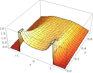
Figure 10. Harmonic extension in the halfplane of the function $\mathbb{R}\ni x\mapsto(1-x^{2})^{-1/2}_{+}$.

The function $U_{-1/2}$ is plotted in Figure 10. We recall that the function $U_{-1/2}$ is well-defined, thanks to (D.6). Also, the denominator never vanishes when $y>0$ and so $U_{-1/2}$ is harmonic in the halfplane, being the real part of a holomorphic function in such domain.

Furthermore, in light of (D.9), we have that

$$\lim_{y\searrow 0}\frac{1}{\displaystyle{\surd}{1-z^{2}}}\,=\,\left\{\begin{matrix}-\displaystyle\frac{i}{\sqrt{|1-x^{2}|}}&{\mbox{ if }}x^{2}>1,\\ \displaystyle\frac{1}{\sqrt{|1-x^{2}|}}&{\mbox{ if }}x^{2}<1,\\ +\infty&{\mbox{ if }}x^{2}=1,\end{matrix}\right.$$

and therefore

$$\lim_{y\searrow 0}U_{-1/2}(x,y)=\Re\left(\lim_{y\searrow 0}\frac{1}{\displaystyle{\surd}{1-z^{2}}}\right)=\left\{\begin{matrix}0&{\mbox{ if }}x^{2}>1,\\ \displaystyle\frac{1}{\sqrt{|1-x^{2}|}}&{\mbox{ if }}x^{2}<1,\\ +\infty&{\mbox{ if }}x^{2}=1,\end{matrix}\right.$$

$$\qquad=(1-x^{2})^{-1/2}_{+}=u_{-1/2}(x).$$

This gives that $U_{-1/2}$ is the harmonic extension of $u_{-1/2}$ to the halfplane. Therefore, by (2.6) (2.7) and (D.14), for any $x\in(-1,1)$ we have that

$$-(-\Delta)^{-1/2}u_{1/2}(x) = \lim_{y\searrow 0}\partial_{y}U_{-1/2}(x,y)$$

$$= \lim_{y\searrow 0}\partial_{y}\left(\Re\left(\frac{1}{\displaystyle{\surd}{1-z^{2}}}\right)\right)$$

$$= \lim_{y\searrow 0}\Re\left(\partial_{y}\left(\frac{1}{\displaystyle{\surd}{1-z^{2}}}\right)\right)$$

$$= -\lim_{y\searrow 0}\Re\left(\left(\frac{1}{\displaystyle{\surd}{1-z^{2}}}\right)^{2}\partial_{y}\left(\displaystyle{\surd}{1-z^{2}}\right)\right)$$

$$= -\frac{1}{1-x^{2}}\lim_{y\searrow 0}\Re\left(\partial_{y}\left(\displaystyle{\surd}{1-z^{2}}\right)\right)$$

$$= 0,$$

that is (2.24).

Appendix I Proof of (2.29) (based on Fourier methods)

When $n=1$, we use (2.28) to find that

(I.1) $$\begin{split}{\mathcal{G}}_{1/2}(x)\;&=\int_{\mathbb{R}}e^{-|\xi|}\,e^{ix\xi}\,d\xi=\lim_{R\to+\infty}\int_{0}^{R}e^{-\xi}\,e^{ix\xi}\,d\xi+\int_{-R}^{0}e^{\xi}\,e^{ix\xi}\,d\xi\\ &=\lim_{R\to+\infty}\frac{e^{R(ix-1)}-1}{ix-1}+\frac{1-e^{-R(ix+1)}}{ix+1}=-\frac{1}{ix-1}+\frac{1}{ix+1}=\frac{2}{x^{2}+1}.\end{split}$$

This proves (2.28) when $n=1$.

Let us now deal with the case $n\geqslant 2$. By changing variable $Y:=1/y$, we see that

$$\int_{0}^{+\infty}e^{-\frac{|\xi|\,\left(y-\frac{1}{y}\right)^{2}}{2}}\,dy=\int_{0}^{+\infty}e^{-\frac{|\xi|\,\left(Y-\frac{1}{Y}\right)^{2}}{2}}\,\frac{dY}{Y^{2}}.$$

Therefore, summing up the left hand side to both sides of this identity and using the transformation $\eta:=y-\frac{1}{y}$,

$$2\int_{0}^{+\infty}e^{-\frac{|\xi|\,\left(y-\frac{1}{y}\right)^{2}}{2}}\,dy = \int_{0}^{+\infty}\left(1+\frac{1}{y^{2}}\right)\,e^{-\frac{|\xi|\,\left(y-\frac{1}{y}\right)^{2}}{2}}\,dy$$

$$= \,{\rm const}\,\int_{0}^{+\infty}e^{-\frac{|\xi|\,\eta^{2}}{2}}\,d\eta$$

$$= \frac{\,{\rm const}\,}{\sqrt{|\xi|}}.$$

As a result,

$$e^{-|\xi|}=\frac{\,{\rm const}\,e^{-|\xi|}\,\sqrt{|\xi|}}{\sqrt{|\xi|}} = \,{\rm const}\,e^{-|\xi|}\,\sqrt{|\xi|}\int_{0}^{+\infty}e^{-\frac{|\xi|\,\left(y-\frac{1}{y}\right)^{2}}{2}}\,dy$$

$$= \,{\rm const}\,e^{-|\xi|}\,\sqrt{|\xi|}\int_{0}^{+\infty}e^{-\frac{|\xi|\,\left(y^{2}+\frac{1}{y^{2}}-2\right)}{2}}\,dy$$

$$= \,{\rm const}\,\sqrt{|\xi|}\int_{0}^{+\infty}e^{-\frac{|\xi|\,\left(y^{2}+\frac{1}{y^{2}}\right)}{2}}\,dy$$

$$= \,{\rm const}\,\int_{0}^{+\infty}\frac{1}{\sqrt{t}}\;e^{-\frac{t}{2}}\,e^{-\frac{|\xi|^{2}}{2t}}\,dt,$$

where the substitution $t:=|\xi|\,y^{2}$ has been used.

Accordingly, by (2.28), the Gaussian Fourier transform and the change of variable $\tau:=t(1+|x|^{2})$,

$${\mathcal{G}}_{1/2}(x) = \int_{\mathbb{R}^{n}}e^{-|\xi|}\,e^{ix\cdot\xi}\,d\xi$$

$$= \,{\rm const}\,\iint_{\mathbb{R}^{n}\times(0,+\infty)}\frac{1}{\sqrt{t}}\;e^{-\frac{t}{2}}\,e^{-\frac{|\xi|^{2}}{2t}}\,e^{ix\cdot\xi}\,d\xi\,dt$$

$$= \,{\rm const}\,\int_{(0,+\infty)}t^{\frac{n-1}{2}}e^{-\frac{t}{2}}\,e^{-\frac{t|x|^{2}}{2}}\,dt$$

$$= \,{\rm const}\,\int_{(0,+\infty)}\left(\frac{\tau}{1+|x|^{2}}\right)^{\frac{n-1}{2}}e^{-\frac{\tau}{2}}\,\frac{d\tau}{1+|x|^{2}}$$

$$= \frac{\,{\rm const}\,}{\big{(}1+|x|^{2}\big{)}^{\frac{n+1}{2}}}.$$

This establishes (2.29).

Appendix J Another proof of (2.29) (based on extension methods)

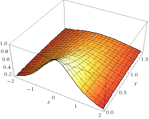
Figure 11. Harmonic extension in the halfplane of the function $\mathbb{R}\ni x\mapsto\frac{1}{1+|x|^{2}}$.

The idea is to consider the fundamental solution in the extended space and take a derivative (the time variable acting as a translation and, to favor the intuition, one may keep in mind that the Poisson kernel is the normal derivative of the Green function). Interestingly, this proof is, in a sense, “conceptually simpler”, and “less technical” than that in Appendix I, thus demonstrating that, at least in some cases, when appropriately used, fractional methods may lead to cultural advantages with respect to more classical approaches.

For this proof, we consider variables $X:=(x,y)\in\mathbb{R}^{n}\times(0,+\infty)\subset\mathbb{R}^{n+1}$ and fix $t>0$. We let $\Gamma$ be the fundamental solution in $\mathbb{R}^{n+1}$, namely

$$\Gamma(X):=\left\{\begin{matrix}-\,{\rm const}\,\log|X|&{\mbox{ if }}n=1,\cr\displaystyle\frac{\,{\rm const}\,}{|X|^{n-1}}&{\mbox{ if }}n\geqslant 2.\end{matrix}\right.$$

By construction $\Delta\Gamma$ is the Delta Function at the origin and so, for any $t>0$, we have that $\tilde{\Gamma}(X;t)=\tilde{\Gamma}(x,y;t):=\Gamma(x,y+t)$ is harmonic for $(x,y)\in\mathbb{R}^{n}\times(0,+\infty)$. Accordingly, the function $U(x,y;t):=\partial_{y}\tilde{\Gamma}(x,y;t)$ is also harmonic for $(x,y)\in\mathbb{R}^{n}\times(0,+\infty)$. We remark that

$$U(x,y;t)=\partial_{y}\Gamma(x,y+t)=\displaystyle\frac{\,{\rm const}\,}{|(x,y+t)|^{n}}\partial_{y}\sqrt{|x|^{2}+(y+t)^{2}}=\displaystyle\frac{\,{\rm const}\,(y+t)}{|(x,y+t)|^{n+1}}=\displaystyle\frac{\,{\rm const}\,(y+t)}{\big{(}|x|^{2}+(y+t)^{2}\big{)}^{\frac{n+1}{2}}}.$$

This function is plotted in Figure 11 (for the model case in the plane). We observe that

$$\lim_{y\searrow 0}U(x,0;t)=\displaystyle\frac{\,{\rm const}\,\;t}{\big{(}|x|^{2}+t^{2}\big{)}^{\frac{n+1}{2}}}=\displaystyle\frac{\,{\rm const}\,}{t^{n}\,\big{(}1+(|x|/t)^{2}\big{)}^{\frac{n+1}{2}}}=:u(x,t).$$

As a consequence, by (2.6) and (2.7) (and noticing that the role played by the variables $y$ and $t$ in the function $U$ is the same),

$$-(-\Delta)^{1/2}u(x,t)=\lim_{y\searrow 0}\partial_{y}U(x,y;t)=\lim_{y\searrow 0}\partial_{y}\displaystyle\frac{\,{\rm const}\,(y+t)}{\big{(}|x|^{2}+(y+t)^{2}\big{)}^{\frac{n+1}{2}}}=\lim_{y\searrow 0}\partial_{t}\displaystyle\frac{\,{\rm const}\,(y+t)}{\big{(}|x|^{2}+(y+t)^{2}\big{)}^{\frac{n+1}{2}}}$$

$$\qquad\qquad=\partial_{t}\displaystyle\frac{\,{\rm const}\,\;t}{\big{(}|x|^{2}+t^{2}\big{)}^{\frac{n+1}{2}}}=\partial_{t}u(x,t).$$

This shows that $u$ solves the fractional heat equation, with $u$ approaching a Delta function when $t\searrow 0$. Hence

$${\mathcal{G}}_{1/2}(x)=u(x,1)=\displaystyle\frac{\,{\rm const}\,}{\big{(}1+|x|^{2}\big{)}^{\frac{n+1}{2}}},$$

that is (2.29).

Appendix K Proof of (2.36)

First, we construct a useful barrier. Given $A>1$, we define

$$w(t):=\left\{\begin{matrix}A&{\mbox{ if }}|t|\leqslant 1,\\ t^{-1-2s}&{\mbox{ if }}|t|>1.\end{matrix}\right.$$

We claim that if $A$ is sufficiently large, then

(K.1) $$(-\Delta)^{s}w(t)<-3w(t)\quad{\mbox{ for all }}t\in\mathbb{R}\setminus(-3,3).$$

To prove this, fix $t\geqslant 3$ (the case $t\leqslant-3$ being similar). Then, if $|\xi-t|<1$, we have that

$$\xi\geqslant t-1=\frac{2t}{3}+\frac{t}{3}-1\geqslant\frac{2t}{3}.$$

As a consequence, if $|\tau-t|<1$,

$$\big{|}w(t)-w(\tau)+\dot{w}(t)(\tau-t)\big{|}\leqslant\sup_{|\xi-t|<1}|\ddot{w}(\xi)|\,|t-\tau|^{2}$$

$$\qquad\leqslant\,{\rm const}\,\sup_{\xi\geqslant 2t/3}\xi^{-3-2s}\,|t-\tau|^{2}\leqslant\,{\rm const}\,t^{-3-2s}\,|t-\tau|^{2}.$$

This implies that

(K.2) $$\begin{split}&\int_{\{|\tau-t|<1\}}\frac{w(t)-w(\tau)}{|t-\tau|^{1+2s}}\,d\tau=\int_{\{|\tau-t|<1\}}\frac{w(t)-w(\tau)+\dot{w}(t)(\tau-t)}{|t-\tau|^{1+2s}}\,d\tau\\ &\qquad\leqslant\,{\rm const}\,t^{-3-2s}\int_{\{|\tau-t|<1\}}\frac{|t-\tau|^{2}}{|t-\tau|^{1+2s}}\,d\tau=\,{\rm const}\,t^{-3-2s}\\ &\qquad\leqslant\,{\rm const}\,t^{-1-2s}=\,{\rm const}\,w(t).\end{split}$$

On the other hand,

(K.3) $$\int_{\{|\tau-t|\geqslant 1\}\cap\{|\tau|>1\}}\frac{w(t)-w(\tau)}{|t-\tau|^{1+2s}}\,d\tau\leqslant\int_{\{|\tau-t|\geqslant 1\}}\frac{w(t)}{|t-\tau|^{1+2s}}\,d\tau\leqslant\,{\rm const}\,w(t).$$

In addition, if $|\tau|\leqslant 1$ then $|\tau-t|\geqslant t-\tau\geqslant 3-1>1$, hence

$$\{|\tau-t|\geqslant 1\}\cap\{|\tau|\leqslant 1\}=\{|\tau|\leqslant 1\}.$$

Accordingly,

(K.4) $$\int_{\{|\tau-t|\geqslant 1\}\cap\{|\tau|\leqslant 1\}}\frac{w(t)-w(\tau)}{|t-\tau|^{1+2s}}\,d\tau=\int_{\{|\tau|\leqslant 1\}}\frac{t^{-1-2s}-A}{|t-\tau|^{1+2s}}\,d\tau\leqslant\int_{\{|\tau|\leqslant 1\}}\frac{1-A}{|t-\tau|^{1+2s}}\,d\tau.$$

We also observe that if $|\tau|\leqslant 1$ then $|t-\tau|\leqslant t+1\leqslant 2t$ and therefore

$$\int_{\{|\tau|\leqslant 1\}}\frac{d\tau}{|t-\tau|^{1+2s}}\geqslant\frac{\,{\rm const}\,}{t^{1+2s}}={\,{\rm const}\,}w(t).$$

So, we plug this information into (K.4), assuming $A>1$ and we obtain that

(K.5) $$\int_{\{|\tau-t|\geqslant 1\}\cap\{|\tau|\leqslant 1\}}\frac{w(t)-w(\tau)}{|t-\tau|^{1+2s}}\,d\tau\leqslant-{(A-1)\,\,{\rm const}\,}w(t).$$

Thus, gathering together the estimates in (K.2), (K.3) and (K.5), we conclude that

$$\int_{\mathbb{R}}\frac{w(t)-w(\tau)}{|t-\tau|^{1+2s}}\,d\tau\leqslant\,{\rm const}\,w(t)-{(A-1)\,\,{\rm const}\,}w(t)\leqslant-4w(t)<-3w(t),$$

as long as $A$ is sufficiently large. This proves (K.1).

Now, to prove (2.36), we define $v:=\dot{u}>0$. From (2.40), we know that

(K.6) $$(-\Delta)^{s}v=(1-3u^{2})v\geqslant-3u^{2}v\geqslant-3v.$$

Given $\varepsilon>0$, we define

$$w_{\varepsilon}(t):=\frac{\iota}{A}\,w(t)-\varepsilon,\qquad{\mbox{ where }}\iota:=\min_{t\in[-3,3]}v(t).$$

We claim that

(K.7) $$w_{\varepsilon}\leqslant v.$$

Indeed, for large $\varepsilon$, it holds that $w_{\varepsilon}<0<v$ and so (K.7) is satisfied. In addition, for any $\varepsilon>0$,

(K.8) $$\lim_{t\to+\infty}w_{\varepsilon}(t)=-\varepsilon<0\leqslant\inf_{t\in\mathbb{R}}v(t).$$

Suppose now that $\varepsilon_{\star}>0$ produces a touching point between $w_{\varepsilon_{\star}}$ and $v$, namely $w_{\varepsilon_{\star}}\leqslant v$ and $w_{\varepsilon_{\star}}(t_{\star})=v(t_{\star})$ for some $t_{\star}\in\mathbb{R}$. Notice that, if $|\tau|\leqslant 3$,

$$w_{\varepsilon_{\star}}(\tau)\leqslant\frac{\iota}{A}\,\sup_{t\in\mathbb{R}}w(t)-\varepsilon\leqslant\iota-\varepsilon=\min_{t\in[-3,3]}v(t)-\varepsilon\leqslant v(\tau)-\varepsilon<v(\tau),$$

and therefore $|t_{\star}|>3$. Accordingly, if we set $v_{\star}:=v-w_{\varepsilon_{\star}}$, using (K.1) and (K.6), we see that

$$0=-3v_{\star}(t_{\star})=-3v(t_{\star})+3w_{\varepsilon_{\star}}(t_{\star})\leqslant(-\Delta)^{s}v(t_{\star})-(-\Delta)^{s}w_{\varepsilon_{\star}}(t_{\star})$$

$$\qquad\quad\qquad=(-\Delta)^{s}v_{\star}(t_{\star})=\int_{\mathbb{R}}\frac{v_{\star}(t_{\star})-v_{\star}(\tau)}{|t_{\star}-\tau|^{1+2s}}\,d\tau=-\int_{\mathbb{R}}\frac{v_{\star}(\tau)}{|t_{\star}-\tau|^{1+2s}}\,d\tau.$$

Since the latter integrand is nonnegative, we conclude that $v_{\star}$ must vanish identically, and thus $w_{\varepsilon_{\star}}$ must coincide with $v$. But this is in contradiction with (K.8) and so the proof of (K.7) is complete.

Then, by sending $\varepsilon\searrow 0$ in (K.7) we find that $v\geqslant\frac{\iota}{A}\,w$, and therefore, for $t\geqslant 1$ we have that $\dot{u}(t)=v(t)\geqslant\kappa t^{-1-2s}$, for all $t>1$, for some $\kappa>0$.

Consequently, for any $t>1$,

$$1-u(t)=\lim_{T\to+\infty}u(T)-u(t)=\lim_{T\to+\infty}\int^{T}_{t}\dot{u}(\tau)\,d\tau=\int^{+\infty}_{t}\dot{u}(\tau)\,d\tau\geqslant\kappa\int^{+\infty}_{t}\tau^{-1-2s}\,d\tau=\frac{\kappa}{2s}\,t^{-2s},$$

and a similar estimates holds for $1+u(t)$ when $t<-1$.

These considerations establish (2.36), as desired.

Appendix L Proof of (2.38)

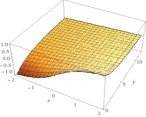
Figure 12. Harmonic extension in the halfplane of the function $\mathbb{R}\ni x\mapsto\frac{2}{\pi}\,\arctan x$.

Here we prove that (2.38) is a solution of (2.37). The idea of the proof, as showed in Figure 12, is to consider the harmonic extension of the function $\mathbb{R}\ni x\mapsto\frac{2}{\pi}\,\arctan x$ in the halfplane $\mathbb{R}\times(0,+\infty)$ and use the method described in (2.6) and (2.7).

We let

$$U(x,y):=\frac{2}{\pi}\arctan\frac{x}{y+1}.$$

The function $U$ is depicted in Figure 12. Of course, it coincides with $u$ when $y=0$ and, for any $x\in\mathbb{R}$ and $y>0$,

(L.1) $$\frac{\pi}{2}\,\Delta U(x,y)=-\frac{2x(1+y)}{(x^{2}+(1+y)^{2})^{2}}+\frac{2x(1+y)}{(x^{2}+(1+y)^{2})^{2}}=0.$$

Hence, the setting in (2.6) is satisfied and so, in light of (2.7). we have

(L.2) $$(-\Delta)^{1/2}u(x)=-\lim_{y\searrow 0}\partial_{y}U(x,y)=\frac{2}{\pi}\lim_{y\searrow 0}\frac{x}{x^{2}+(1+y)^{2}}=\frac{2x}{\pi\,(x^{2}+1)}$$

Also, by the trigonometric Double-angle Formula, for any $\theta\in\left(-\frac{\pi}{2},\frac{\pi}{2}\right)$,

$$\sin(2\theta)=2\sin\theta\cos\theta={\frac{2\tan\theta}{\tan^{2}\theta+1}}.$$

Hence, taking $\theta:=\arctan x$,

$$\sin(\pi u(x))=\sin(2\arctan x)={\frac{2x}{x^{2}+1}}.$$

This and (L.2) show that (2.38) is a solution of (2.37).

Appendix M Another proof of (2.38) (based on (2.29))

This proof of (2.38) is based on the fractional heat kernel in (2.29). This approach has the advantage of being quite general (see e.g. Theorem 3.1 in [MR3280032]) and also to relate the two “miraculous” explicit formulas (2.29) and (2.38), which are available only in the special case $s=1/2$.

For this, we let $P=P(x,t)$ the fundamental solution of the heat flow in (2.25) with $n=1$ and $s=1/2$. Notice that, by (2.29), we know that

(M.1) $$P(x,1)={\mathcal{G}}_{1/2}(x)=\frac{c}{1+x^{2}},$$

with

$$c:=\left(\int_{\mathbb{R}}\frac{dx}{1+x^{2}}\right)^{-1}=\frac{1}{\pi}.$$

Also, by scaling,

(M.2) $$P(x,t)=t^{-1}P(t^{-1}x,1)=t^{-1}{\mathcal{G}}_{1/2}(t^{-1}x).$$

For any $x\in\mathbb{R}$ and any $t>0$, we define

(M.3) $$U(x,t):=2\int_{0}^{x}P(\eta,t+1)\,d\eta.$$

In light of (M.2), we see that

$$|U(x,t)|\leqslant 2(t+1)^{-1}\int_{0}^{x}{\mathcal{G}}_{1/2}\big{(}(t+1)^{-1}\eta\big{)}\,d\eta=2\int_{0}^{(t+1)^{-1}x}{\mathcal{G}}_{1/2}(\zeta)\,d\zeta,$$

which is bounded in $\mathbb{R}\times[0,+\infty)$, and infinitesimal as $t\to+\infty$ for any fixed $x\in\mathbb{R}$.

Notice also that

$$\partial^{2}_{t}P=\partial_{t}(\partial_{t}P)=\partial_{t}(-\Delta)^{1/2}P=(-\Delta)^{1/2}\partial_{t}P=(-\Delta)^{1/2}(-\Delta)^{1/2}P=-\partial^{2}_{x}P,$$

by (2.5). As a consequence,

(M.4) $$\begin{split}\frac{1}{2}(\partial^{2}_{x}+\partial^{2}_{t})U(x,t)\,&=\partial_{x}P(x,t+1)+\int_{0}^{x}\partial^{2}_{t}P(\eta,t+1)\,d\eta\\ &=\partial_{x}P(x,t+1)-\int_{0}^{x}\partial^{2}_{x}P(\eta,t+1)\,d\eta\\ &=\partial_{x}P(0,t+1)\\ &=0,\end{split}$$

where the last identity follows from (M.2).

Besides, from (M.2) we have that

$$\partial_{t}P(x,t)=\partial_{t}\Big{(}t^{-1}{\mathcal{G}}_{1/2}(t^{-1}x)\Big{)}=-t^{-2}{\mathcal{G}}_{1/2}(t^{-1}x)-t^{-3}x{\mathcal{G}}_{1/2}^{\prime}(t^{-1}x)$$

and so

$$-\partial_{t}P(x,1)={\mathcal{G}}_{1/2}(x)+x{\mathcal{G}}_{1/2}^{\prime}(x)=\partial_{x}\big{(}x\,{\mathcal{G}}_{1/2}(x)\big{)}.$$

In view of this, we have that

(M.5) $$\partial_{t}U(x,0)=2\int_{0}^{x}\partial_{t}P(\eta,1)\,d\eta=2\int_{0}^{x}\partial_{\eta}\big{(}\eta\,{\mathcal{G}}_{1/2}(\eta)\big{)}\,d\eta=2x\,{\mathcal{G}}_{1/2}(x).$$

Accordingly, from (M.4) and (M.5), using the extension method in (2.6) and (2.7) (with the variable $y$ called $t$ here), we conclude that, if

$$u(x):=U(x,0),$$

then

(M.6) $$(-\Delta)^{1/2}u(x)=2x\,{\mathcal{G}}_{1/2}(x).$$

We remark that, by (M.1) and (M.3),

(M.7) $$u(x)=2c\int_{0}^{x}\frac{d\eta}{1+x^{2}}=\frac{2}{\pi}\,\arctan x.$$

This, (M.1) and (M.6) give that

$$(-\Delta)^{1/2}u(x)=\frac{1}{\pi}\,\frac{2x}{1+x^{2}}=\frac{1}{\pi}\,\sin(2\arctan x)=\frac{1}{\pi}\,\sin\big{(}\pi u(x)\big{)},$$

that is (2.38), as desired.

Appendix N Proof of (2.46)

Due to translation invariance, we can reduce ourselves to proving (2.46) at the origin. We consider a measurable $u:\mathbb{R}^{n}\to\mathbb{R}$ such that

$$\int_{\mathbb{R}^{n}}\frac{|u(y)|}{1+|y|^{n+2}}\ <\ +\infty.$$

Assume first that

(N.1) $$u(x)=0 x\in B_{r}$$ for any ,

for some $r>0$. As a matter of fact, under these assumptions on $u$, the right-hand side of (2.46) vanishes at $0$ regardless the size of $r$. Indeed,

$${\phantom{=}}\ \left.\int_{\mathbb{R}^{n}}\frac{u(x+2y)+u(x-2y)-4u(x+y)-4u(x-y)+6u(x)}{{|y|}^{n+2}}\;dy\right|_{x=0}$$

$$=\ \int_{\mathbb{R}^{n}}\frac{u(2y)+u(-2y)-4u(y)-4u(-y)}{{|y|}^{n+2}}\;dy\ =\ 2\int_{\mathbb{R}^{n}\setminus B_{r/2}}\frac{u(2y)}{{|y|}^{n+2}}\;dy-8\int_{\mathbb{R}^{n}\setminus B_{r}}\frac{u(y)}{{|y|}^{n+2}}\;dy$$

$$=\ 2\int_{\mathbb{R}^{n}\setminus B_{r}}\frac{2^{n+2}\,u(Y)}{2^{n}\,{|Y|}^{n+2}}\;dY-8\int_{\mathbb{R}^{n}\setminus B_{r}}\frac{u(y)}{{|y|}^{n+2}}\;dy\ =\ 0.$$

This proves (2.46) under the additional assumption in (N.1), that we are now going to remove. To this end, for $r\in(0,1)$, denote by $\chi_{r}$ the characteristic function of $B_{r}$, i.e. $\chi_{r}(x)=1$ if $x\in B_{r}$ and $\chi_{r}(x)=0$ otherwise. Consider now $u\in C^{2,\alpha}(B_{r})$, for some $\alpha\in(0,1)$, with

(N.2) $$u(0)=|\nabla u(0)|=0$$

for simplicity (note that one can always modify $u$ by considering $\tilde{u}(x)=u(x)-u(0)-\nabla u(0)\cdot x$ and without affecting the operators in (2.46)). Then, the right hand side of (2.46) becomes in this case

$$\phantom{=}\ \int_{\mathbb{R}^{n}}\frac{u(2y)+u(-2y)-4u(y)-4u(-y)}{{|y|}^{n+2}}\;dy\ =\ 2\int_{\mathbb{R}^{n}}\frac{u(2y)-4u(y)}{{|y|}^{n+2}}\;dy\ =$$

$$=\ 2\int_{\mathbb{R}^{n}}\frac{u(2y)\chi_{r}(2y)-4u(y)\chi_{r}(y)}{{|y|}^{n+2}}\;dy\ +\ 2\int_{\mathbb{R}^{n}}\frac{u(2y)(1-\chi_{r}(2y))-4u(y)(1-\chi_{r}(y))}{{|y|}^{n+2}}\;dy.$$

The second addend is trivial for any $r\in(0,1)$, in view of the above remark, since $u(1-\chi_{r})$ is constantly equal to $0$ in $B_{r}$. For the first one, we have

(N.3) $$\int_{\mathbb{R}^{n}}\frac{u(2y)\chi_{r}(2y)-4u(y)\chi_{r}(y)}{{|y|}^{n+2}}\;dy\ =\ \int_{B_{r/2}}\frac{u(2y)-4u(y)}{{|y|}^{n+2}}\;dy-4\int_{B_{r}\setminus B_{r/2}}\frac{u(y)}{{|y|}^{n+2}}\;dy.$$

Now, we recall (N.2) and we notice that

$$|u(2y)-4u(y)|\leqslant\|u\|_{C^{2,\alpha}(B)}|y|^{2+\alpha},$$

which in turn implies that

(N.4) $$\left|\int_{B_{r/2}}\frac{u(2y)-4u(y)}{{|y|}^{n+2}}\;dy\right|\ \leqslant\ \,{\rm const}\,\|u\|_{C^{2,\alpha}(B)}r^{\alpha}.$$

On the other hand, a Taylor expansion and (N.2) yield

(N.5) $$\begin{split}&{\phantom{=}}\ \int_{B_{r}\setminus B_{r/2}}\frac{u(y)}{{|y|}^{n+2}}\;dy\ =\ \int_{r/2}^{r}\frac{1}{\rho^{n+2}}\int_{\partial B_{\rho}}u(y)\;dy\;d\rho\ \\ &=\ \int_{r/2}^{r}\frac{1}{\rho^{3}}\int_{\partial B_{1}}u(\rho\theta)\;d\theta\;d\rho\ =\ \int_{r/2}^{r}\frac{1}{2\rho}\int_{\partial B_{1}}\left(D^{2}u(0)\theta\cdot\theta+\eta(\rho\theta)\right)\;d\theta\;d\rho\\ &=\ \,{\rm const}\,\Delta u(0)+\int_{r/2}^{r}\frac{1}{2\rho}\int_{\partial B_{1}}\eta(\rho\theta)\;d\theta\;d\rho\end{split}$$

in view of (1.1), for some $\eta:B_{r}\to\mathbb{R}$ such that $|\eta(x)|\leqslant c|x|^{\alpha}$. From this, (N.3) and (N.4) we deduce that

$$\int_{\mathbb{R}^{n}}\frac{u(2y)+u(-2y)-4u(y)-4u(-y)}{{|y|}^{n+2}}\;dy\ =\ -\,{\rm const}\,\lim_{r\searrow 0}\int_{B_{r}\setminus B_{r/2}}\frac{u(y)}{{|y|}^{n+2}}\;dy\ =\ -\,{\rm const}\,\Delta u(0)$$

which finally justifies (2.46).

It is interesting to remark that the main contribution to prove (2.46) comes in this case from the “intermediate ring” in (N.5).

Appendix O Proof of (2.48)

Take for instance $\Omega$ to be the unit ball and $\bar{u}=1-|x|^{2}$. Suppose that $\|\bar{u}-v_{\varepsilon}\|_{C^{2}(\Omega)}\leqslant\varepsilon$. Then, for small $\varepsilon$, if $x\in\mathbb{R}^{n}\setminus B_{1/2}$ it holds that

$$v_{\varepsilon}(x)\leqslant\bar{u}(x)+\varepsilon=1-|x|^{2}+\varepsilon\leqslant\frac{3}{4}+\varepsilon\leqslant\frac{4}{5},$$

while

$$v_{\varepsilon}(0)\geqslant\bar{u}(0)-\varepsilon=1-\varepsilon\geqslant\frac{5}{6}.$$

This implies that there exists $x_{\varepsilon}\in\overline{B_{1/2}}$ such that

$$v_{\varepsilon}(x_{\varepsilon})=\sup_{B_{1}}v_{\varepsilon}\geqslant\frac{5}{6}>\frac{4}{5}\geqslant\sup_{B_{1}\setminus B_{1/2}}v_{\varepsilon}.$$

As a result,

$$\,{\rm P.V.}\,\int_{\Omega}\frac{v_{\varepsilon}(x_{\varepsilon})-v_{\varepsilon}(y)}{|x_{\varepsilon}-y|^{n+2s}}\,dy\geqslant\int_{B_{1}\setminus B_{3/4}}\frac{v_{\varepsilon}(x_{\varepsilon})-v_{\varepsilon}(y)}{|x_{\varepsilon}-y|^{n+2s}}\,dy\geqslant\int_{B_{1}\setminus B_{3/4}}\left(\frac{5}{6}-\frac{4}{5}\right)\,dy\geqslant\,{\rm const}\,.$$

This says that $(-\Delta)^{s}v_{\varepsilon}$ cannot vanish at $x_{\varepsilon}$ and so (2.48) is proved.

Appendix P Proof of (2.52)

Let us first notice that the identity

(P.1) $$\lambda^{s}\ =\ \frac{s}{\Gamma(1-s)}\int_{0}^{\infty}\frac{1-e^{-t\lambda}}{t^{1+s}}\;dt$$

holds for any $\lambda>0$ and $s\in(0,1)$, because

$$\int_{0}^{\infty}\frac{1-e^{-t}}{t^{1+s}}\;dt=\left.\frac{1-e^{-t}}{-s\,t^{s}}\right|_{0}^{\infty}+\frac{1}{s}\int_{0}^{\infty}\frac{e^{-t}}{t^{s}}\;dt=\frac{\Gamma(1-s)}{s}.$$

We also observe that when $u\in C^{\infty}_{0}(\Omega)$, the coefficients $\hat{u}_{j}$ decay fast as $j\to\infty$: indeed

$$\hat{u}_{j}=-\frac{1}{\mu_{j}}\int_{\Omega}u\,\Delta\psi_{j}=-\frac{1}{\mu_{j}}\int_{\Omega}\psi_{j}\,\Delta u=\ldots=(-1)^{k}\frac{1}{\mu_{j}^{k}}\int_{\Omega}\psi_{j}\,\Delta^{k}u.$$

Therefore, applying equality (P.1) to the $\mu_{j}$’s in (2.51) we obtain

(P.2) $${(-\Delta)^{s}_{N,\Omega}}u\ =\ \frac{s}{\Gamma(1-s)}\sum_{j=0}^{+\infty}\int_{0}^{\infty}\frac{\hat{u}_{j}\psi_{j}-e^{-t\mu_{j}}\hat{u}_{j}\psi_{j}}{t^{1+s}}\;dt=\frac{s}{\Gamma(1-s)}\int_{0}^{\infty}\frac{u-e^{t{\Delta_{N,\Omega}}u}}{t^{1+s}}\;dt,\quad u\in C^{\infty}_{0}(\Omega)$$

where $\{e^{t\Delta_{N,\Omega}}\}_{t>0}$ stands for the heat semigroup associated to ${\Delta_{N,\Omega}}$. i.e. $e^{t{\Delta_{N,\Omega}}}u$ solves

$$\left\{\begin{matrix}\partial_{t}v(x,t)=\Delta v(x,t){\mbox{ in }}\Omega\times(0,\infty)\\ \partial_{\nu}v(x,t)=0\text{ on }\partial\Omega\times(0,\infty)\\ v(x,0)=u(x)\text{ on }\Omega\times\{0\}.\end{matrix}\right.$$

To check (P.2), it is sufficient to notice that

$$\partial_{t}\left(\sum_{j=0}^{+\infty}e^{-t\mu_{j}}\hat{u}_{j}\psi_{j}\right)=-\sum_{j=0}^{+\infty}\mu_{j}e^{-t\mu_{j}}\hat{u}_{j}\psi_{j}=\sum_{j=0}^{+\infty}e^{-t\mu_{j}}\hat{u}_{j}\Delta\psi_{j}=\Delta\left(\sum_{j=0}^{+\infty}e^{-t\mu_{j}}\hat{u}_{j}\psi_{j}\right)$$

and that

$$\left.\left(\sum_{j=0}^{+\infty}e^{-t\mu_{j}}\hat{u}_{j}\psi_{j}\right)\right|_{t=0}=\sum_{j=0}^{+\infty}\hat{u}_{j}\psi_{j}=u.$$

Under suitable regularity assumptions on $\Omega$, write now the heat semigroup in terms of the heat kernel $p_{N}^{\Omega}$ as

(P.3) $$e^{t{\Delta_{N,\Omega}}}u(x)\ =\ \int_{\Omega}p_{{N}}^{\Omega}(t,x,y)\,u(y)\;dy,\qquad x\in\Omega,\ t>0$$

where the following two-sided estimate on $p_{{N}}^{\Omega}$ holds (see, for example, [MR2648271, Theorem 3.1])

(P.4) $$\frac{c_{1}\>e^{-c_{2}|x-y|^{2}/t}}{t^{n/2}}\ \leqslant\ p_{{N}}^{\Omega}(t,x,y)\ \leqslant\ \frac{c_{3}\>e^{-c_{4}|x-y|^{2}/t}}{t^{n/2}},\qquad x,y\in\Omega,\ t,c_{1},c_{2},c_{3},c_{4}>0.$$

Recall also that $p_{N}^{\Omega}(t,x,y)=p_{N}^{\Omega}(t,y,x)$ for any $t>0$ and $x,y\in\Omega$, and that

(P.5) $$\int_{\Omega}p_{{N}}^{\Omega}(t,x,y)\;dy\ =\ 1,\qquad x\in\Omega,\ t>0,$$

which follows from noticing that, for any $u\in C^{\infty}_{0}(\Omega)$,

$$\partial_{t}\int_{\Omega}e^{t{\Delta_{N,\Omega}}}u=\int_{\Omega}\partial_{t}e^{t{\Delta_{N,\Omega}}}u=\int_{\Omega}\Delta e^{t{\Delta_{N,\Omega}}}u=-\int_{\partial\Omega}\partial_{\nu}e^{t{\Delta_{N,\Omega}}}u=0$$

and therefore

$$\int_{\Omega}u(x)\;dx=\int_{\Omega}e^{t{\Delta_{N,\Omega}}}u(x)\;dx=\int_{\Omega}\int_{\Omega}p_{{N}}^{\Omega}(t,x,y)\,u(y)\;dy\;dx=\int_{\Omega}u(y)\int_{\Omega}p_{N}^{\Omega}(t,x,y)\;dx\;dy.$$

By (P.5), for any $x\in\Omega$ and $t>0$,

$$u(x)-e^{t{\Delta_{N,\Omega}}}u(x)=\int_{\Omega}p_{{N}}^{\Omega}(t,x,y)\left(u(x)-u(y)\right)dy$$

and, exchanging the order of integration in (P.2) (see below for a justification of this passage), one gets

$${(-\Delta)^{s}_{N,\Omega}}u(x)=\frac{s}{\Gamma(1-s)}\int_{0}^{\infty}\frac{u(x)-e^{t{\Delta_{N,\Omega}}}u(x)}{t^{1+s}}\;dy=\frac{s}{\Gamma(1-s)}\int_{0}^{\infty}\frac{\int_{\Omega}p_{{N}}^{\Omega}(t,x,y)\left(u(x)-u(y)\right)dy}{t^{1+s}}\;dt$$

$$=\frac{s}{\Gamma(1-s)}\;\,{\rm P.V.}\,\int_{\Omega}\left(u(x)-u(y)\right)\int_{0}^{\infty}\frac{p_{{N}}^{\Omega}(t,x,y)}{t^{1+s}}\;dt\;dy=\,{\rm P.V.}\,\int_{\Omega}\frac{\left(u(x)-u(y)\right)k(x,y)}{{|x-y|}^{n+2s}}\;dy,$$

where, in view of (P.4), we have

$$k(x,y):=\frac{s}{\Gamma(1-s)}\;|x-y|^{n+2s}\int_{0}^{\infty}\frac{p_{{N}}^{\Omega}(t,x,y)}{t^{1+s}}\;dt\simeq|x-y|^{n+2s}\int_{0}^{\infty}\frac{e^{-|x-y|^{2}/t}}{t^{n/2+1+s}}\,dt\simeq\int_{0}^{\infty}\frac{e^{-1/t}}{t^{n/2+1+s}}\,dt\simeq 1.$$

These considerations establish (2.52). Note however that in the above computations there is a limit exiting the integral in the $t$ variable, namely:

(P.6) $$\int_{0}^{\infty}\frac{\int_{\Omega}p_{{N}}^{\Omega}(t,x,y)\left(u(x)-u(y)\right)dy}{t^{1+s}}\;dt=\lim_{\varepsilon\searrow 0}\int_{0}^{\infty}\frac{\int_{\Omega\setminus B_{\varepsilon}(x)}p_{{N}}^{\Omega}(t,x,y)\left(u(x)-u(y)\right)dy}{t^{1+s}}\;dt.$$

To properly justify this we are going to build an integrable majorant in $t$ and independent of $\varepsilon$ of the integrand

(P.7) $$\frac{\int_{\Omega\setminus B_{\varepsilon}(x)}p_{{N}}^{\Omega}(t,x,y)\left(u(x)-u(y)\right)dy}{t^{1+s}}.$$

To this end, first of all we observe that, by the boundedness of $u$ and (P.5),

$$\left|\frac{\int_{\Omega\setminus B_{\varepsilon}(x)}p_{{N}}^{\Omega}(t,x,y)\left(u(x)-u(y)\right)dy}{t^{1+s}}\right|\leqslant\frac{2\|u\|_{L^{\infty}(\Omega)}}{t^{1+s}}\int_{\Omega\setminus B_{\varepsilon}(x)}p_{{N}}^{\Omega}(t,x,y)\;dy\leqslant\frac{2\|u\|_{L^{\infty}(\Omega)}}{t^{1+s}}$$

which is integrable at infinity. So, to obtain an integrable bound for (P.7), we can now focus on small values of $t$, say $t\in(0,1)$. For this, we denote by $p$ the heat kernel in $\mathbb{R}^{N}$ and we write

$$\int_{\Omega\setminus B_{\varepsilon}(x)}p_{{N}}^{\Omega}(t,x,y)\left(u(x)-u(y)\right)dy\ =\\ =\ \int_{\Omega\setminus B_{\varepsilon}(x)}p(t,x,y)\left(u(x)-u(y)\right)dy-\int_{\Omega\setminus B_{\varepsilon}(x)}(p_{{N}}^{\Omega}(t,x,y)-p(t,x,y))(u(x)-u(y))\;dy=:A+B.$$

We first manipulate $A$. We reformulate $u$ as

$$u(y)=u(x)+\nabla u(x)\cdot(y-x)+\eta(y)|x-y|^{2},\qquad y\in\mathbb{R}^{n},\ \|\eta\|_{L^{\infty}(\mathbb{R}^{n})}\leqslant\|u\|_{C^{2}(\Omega)},$$

so that

(P.8) $$\begin{split}&\int_{\Omega\setminus B_{\varepsilon}(x)}p(t,x,y)\left(u(x)-u(y)\right)dy=\int_{\mathbb{R}^{n}\setminus B_{\varepsilon}(x)}p(t,x,y)\left(u(x)-u(y)\right)dy-u(x)\int_{\mathbb{R}^{n}\setminus\Omega}p(t,x,y)\;dy\\ &=\int_{\mathbb{R}^{n}\setminus B_{\varepsilon}(x)}p(t,x,y)\nabla u(x)\cdot(x-y)\;dy-\int_{\mathbb{R}^{n}\setminus B_{\varepsilon}(x)}p(t,x,y)\,\eta(y)|x-y|^{2}\;dy-u(x)\int_{\mathbb{R}^{n}\setminus\Omega}p(t,x,y)\;dy.\end{split}$$

In the last expression, the first integral on the right-hand side is $0$ by odd symmetry, while for the second one

(P.9) $$\begin{split}&\left|\int_{\mathbb{R}^{n}\setminus B_{\varepsilon}(x)}p(t,x,y)\,\eta(y)|x-y|^{2}\;dy\right|\leqslant\|u\|_{C^{2}(\Omega)}\int_{\mathbb{R}^{n}\setminus B_{\varepsilon}(x)}p(t,x,y)|x-y|^{2}\;dy\\ &\leqslant\,{\rm const}\,\|u\|_{C^{2}(\Omega)}t^{-/2}\int_{\mathbb{R}^{n}\setminus B_{\varepsilon}(x)}e^{-|x-y|^{2}/(4t)}|x-y|^{2}\;dy\leqslant\,{\rm const}\,\|u\|_{C^{2}(\Omega)}t\int_{\mathbb{R}^{n}\setminus B_{\varepsilon/\sqrt{4t}}}e^{-|z|^{2}}|z|^{2}\;dz\\ &\leqslant\,{\rm const}\,\|u\|_{C^{2}(\Omega)}t.\end{split}$$

As for the last integral in (P.8), we have that

(P.10) $$\begin{split}&|u(x)|\int_{\mathbb{R}^{n}\setminus\Omega}p(t,x,y)\;dy\leqslant\,{\rm const}\,|u(x)|t^{-n/2}\int_{\mathbb{R}^{n}\setminus\Omega}e^{-|x-y|^{2}/(4t)}\;dy\leqslant\\ &\leqslant\,{\rm const}\,|u(x)|t^{-n/2}\int_{\mathbb{R}^{n}\setminus B_{\text{dist}(x,\partial\Omega)}}e^{-|y|^{2}/(4t)}\;dy\leqslant\,{\rm const}\,|u(x)|\int_{\mathbb{R}^{n}\setminus B_{\text{dist}(x,\partial\Omega)/\sqrt{4t}}}e^{-|z|^{2}}\;dz\\ &\leqslant\,{\rm const}\,|u(x)|e^{-\text{dist}(x,\partial\Omega)/\sqrt{4t}}.\end{split}$$

Equations (P.9) and (P.10) imply that

$$\frac{|A|}{t^{1+s}}\leqslant\,{\rm const}\,t^{-s},\qquad t\in(0,1),$$

which is integrable for $t\in(0,1)$.

We turn now to the estimation of $B$ which we rewrite as

$$B=\int_{\Omega}\big{(}p_{{N}}^{\Omega}(t,x,y)-p(t,x,y)\big{)}\big{(}u(x)-u(y)\big{)}\chi_{\Omega\setminus B_{\varepsilon}(x)}(y)\;dy$$

where $\chi_{U}$ stands for the characteristic function of a set $U\subset\mathbb{R}^{n}$. By definition, $B$ solves the heat equation in $\Omega$ with zero initial condition. Moreover, since $u$ is supported in a compact subset $K$ of $\Omega$, $B$ is satisfying the (lateral) boundary condition

$$\Big{|}B\big{|}_{\partial B}\Big{|}\leqslant\int_{\Omega}\big{|}p_{{N}}^{\Omega}(t,x,y)-p(t,x,y)\big{|}|u(y)|\chi_{\Omega\setminus B_{\varepsilon}(x)}(y)\;dy\leqslant\,{\rm const}\,t^{-n/2}\int_{K}e^{-c_{1}|x-y|^{2}/t}|u(y)|\;dy$$

$$\leqslant\,{\rm const}\,\|u\|_{L^{1}(\Omega)}t^{-n/2}e^{-c_{2}/t}$$

for some $c_{1},c_{2}>0$, in view of (P.4) and that, for $x\in\partial\Omega$ and $y\in K$, $|x-y|\geqslant\text{dist}(K,\partial\Omega)>0$. Then, by the parabolic maximum principle (see, for example, Section 7.1.4 in [MR1625845]),

$$\frac{|B|}{t^{1+s}}\leqslant\,{\rm const}\,t^{-n/2-1-s}e^{-c_{2}/t},$$

which again is integrable for $t\in(0,1)$. These observations provide an integrable bound for the integrand in (P.8), thus completing the justification of the claim in (P.6), as desired.

Appendix Q Proof of (2.53)

If $u$ is periodic, we can write it in Fourier series as

$$u(x)=\sum_{k\in\mathbb{Z}^{n}}u_{k}\,e^{2\pi ik\cdot x},$$

and the Fourier basis is also a basis of eigenfunctions. We have that

$$\int_{\mathbb{R}^{n}}\frac{u(x+y)+u(x-y)-2u(x)}{|y|^{n+2s}}\,dy=\sum_{k\in\mathbb{Z}^{n}}\int_{\mathbb{R}^{n}}\frac{u_{k}e^{2\pi ik\cdot(x+y)}+u_{k}e^{2\pi ik\cdot(x-y)}-2u_{k}e^{2\pi ik\cdot x}}{|y|^{n+2s}}\,dy$$

$$\qquad=\sum_{k\in\mathbb{Z}^{n}}u_{k}e^{2\pi ik\cdot x}\int_{\mathbb{R}^{n}}\frac{e^{2\pi ik\cdot y}+e^{-2\pi ik\cdot y}-2}{|y|^{n+2s}}\,dy=\sum_{k\in\mathbb{Z}^{n}}u_{k}e^{2\pi ik\cdot x}\,|k|^{2s}\int_{\mathbb{R}^{n}}\frac{e^{2\pi i\frac{k}{|k|}\cdot Y}+e^{-2\pi i\frac{k}{|k|}\cdot Y}-2}{|Y|^{n+2s}}\,dY$$

$$\qquad=\sum_{k\in\mathbb{Z}^{n}}u_{k}e^{2\pi ik\cdot x}\,|k|^{2s}\int_{\mathbb{R}^{n}}\frac{e^{2\pi iY_{1}}+e^{-2\pi iY_{1}}-2}{|Y|^{n+2s}}\,dY=\,{\rm const}\,\sum_{k\in\mathbb{Z}^{n}}u_{k}e^{2\pi ik\cdot x}\,|k|^{2s}$$

and this shows (2.53).

Appendix R Proof of (2.54)

We fix $\bar{k}\in\mathbb{N}$. We consider the $\bar{k}$th eigenvalue $\lambda_{\bar{k}}>0$ and the corresponding normalized eigenfunction $\phi_{\bar{k}}=:\bar{u}$. We argue by contradiction and suppose that for any $\varepsilon>0$ we can find $v_{\varepsilon}$ such that $\|\bar{u}-v_{\varepsilon}\|_{C^{2}(B_{1})}\leqslant\varepsilon$, with $(-\Delta)^{s}_{D,\Omega}v_{\varepsilon}=0$ in $B_{1}$.

Using the notation in (2.49), we have that $\bar{u}_{k}=\delta_{k\bar{k}}$ and therefore

(R.1) $$\begin{split}&\left\|(-\Delta)^{s}_{D,\Omega}\bar{u}-(-\Delta)^{s}_{D,\Omega}v_{\varepsilon}\right\|^{2}_{L^{2}(\Omega)}=\left\|(-\Delta)^{s}_{D,\Omega}\bar{u}\right\|^{2}_{L^{2}(\Omega)}=\left\|(-\Delta)^{s}_{D,\Omega}\phi_{\bar{k}}\right\|^{2}_{L^{2}(\Omega)}\\ &\qquad=\left\|\lambda_{\bar{k}}^{s}\,\phi_{\bar{k}}\right\|^{2}_{L^{2}(\Omega)}=\lambda_{\bar{k}}^{2s}.\end{split}$$

Furthermore

$$\left\|(-\Delta)^{s}_{D,\Omega}\bar{u}-(-\Delta)^{s}_{D,\Omega}v_{\varepsilon}\right\|^{2}_{L^{2}(\Omega)}=\left\|(-\Delta)^{s}_{D,\Omega}(\bar{u}-v_{\varepsilon})\right\|^{2}_{L^{2}(\Omega)}=\left\|\sum_{k=0}^{+\infty}\lambda_{k}^{s}(\bar{u}-v_{\varepsilon})_{k}\,\phi_{k}\right\|^{2}_{L^{2}(\Omega)}$$

$$\qquad\qquad=\sum_{k=0}^{+\infty}\lambda_{k}^{2s}(\bar{u}-v_{\varepsilon})_{k}^{2}\leqslant\,{\rm const}\,\sum_{k=0}^{+\infty}\lambda_{k}^{2}(\bar{u}-v_{\varepsilon})_{k}^{2}=\,{\rm const}\,\left\|\Delta(\bar{u}-v_{\varepsilon})\right\|^{2}_{L^{2}(\Omega)}$$

$$\qquad\qquad\leqslant\,{\rm const}\,\|\bar{u}-v_{\varepsilon}\|^{2}_{C^{2}(\Omega)}\leqslant\,{\rm const}\,\varepsilon.$$

Comparing this with (R.1), we obtain that $\lambda_{\bar{k}}^{2s}\leqslant\,{\rm const}\,\varepsilon$, which is a contradiction for small $\varepsilon$. Hence, the proof of (2.54) is complete.

Appendix S Proof of (2.60)

Let

$$v(t):=\int_{0}^{t}\frac{\dot{u}(\tau)}{(t-\tau)^{s}}\,d\tau.$$

Then, by (2.59) and writing $\vartheta:=\omega\,({t-\tau})$, we see that

$${\mathcal{L}}v(\omega) = \int_{0}^{+\infty}\left[\int_{0}^{t}\frac{\dot{u}(\tau)}{(t-\tau)^{s}}\,d\tau\right]e^{-\omega t}\,dt=\int_{0}^{+\infty}\left[\int_{\tau}^{+\infty}\frac{\dot{u}(\tau)e^{-\omega t}}{(t-\tau)^{s}}\,dt\right]\,d\tau$$

$$= \omega^{s-1}\int_{0}^{+\infty}\left[\int_{0}^{+\infty}\frac{\dot{u}(\tau)e^{-\omega\tau}\,e^{-\vartheta}}{\vartheta^{s}}\,d\vartheta\right]\,d\tau=\Gamma(1-s)\,\omega^{s-1}\int_{0}^{+\infty}\dot{u}(\tau)e^{-\omega\tau}\,d\tau$$

$$= \Gamma(1-s)\,\omega^{s-1}\int_{0}^{+\infty}\left(\frac{d}{d\tau}\big{(}u(\tau)e^{-\omega\tau}\big{)}+\omega u(\tau)e^{-\omega\tau}\right)\,d\tau$$

$$= \Gamma(1-s)\,\omega^{s-1}\left(-u(0)+\omega\int_{0}^{+\infty}u(\tau)e^{-\omega\tau}\,d\tau\right)$$

$$= \Gamma(1-s)\,\omega^{s-1}\left(-u(0)+\omega{\mathcal{L}}u(\omega)\right),$$

where $\Gamma$ denotes here the Euler’s Gamma Function. This and (2.56) give (2.60), up to neglecting normalizing constants, as desired.

It is also worth pointing out that, as $s\nearrow 1$, formula (2.60) recovers the classical derivative, since, by (2.59),

$${\mathcal{L}}\dot{u}(\omega) = \int_{0}^{+\infty}\dot{u}(t)e^{-\omega t}\,dt$$

$$= \int_{0}^{+\infty}\left(\frac{d}{dt}\big{(}u(t)e^{-\omega t}\big{)}+\omega u(t)e^{-\omega t}\right)\,dt$$

$$= -u(0)+\omega\int_{0}^{+\infty}u(t)e^{-\omega t}\,dt$$

$$= -u(0)+\omega\,{\mathcal{L}}u(\omega),$$

which is (2.60) when $s=1$.

Appendix T Proof of (2.61)

First, we compute the Laplace Transform of the constant function. Namely, by (2.59), for any $b\in\mathbb{R}$,

(T.1) $${\mathcal{L}}b(\omega)=b\,\int_{0}^{+\infty}e^{-\omega t}\,dt=\frac{b}{\omega}.$$

We also set

$$\Psi(t):=\int_{0}^{t}\frac{f(\tau)}{(t-\tau)^{1-s}}\,d\tau$$

and we use (2.59) and the substitution $\vartheta:=\omega\,({t-\tau})$ to calculate that

$${\mathcal{L}}\Psi(\omega) = \int_{0}^{+\infty}\left[\int_{0}^{t}\frac{f(\tau)}{(t-\tau)^{1-s}}\,d\tau\right]\,e^{-\omega t}\,dt$$

$$= \int_{0}^{+\infty}\left[\int_{\tau}^{+\infty}\frac{f(\tau)\,e^{-\omega t}}{(t-\tau)^{1-s}}\,dt\right]\,d\tau$$

$$= \omega^{-s}\int_{0}^{+\infty}\left[\int_{0}^{+\infty}\frac{f(\tau)\,e^{-\omega\tau}\,e^{-\vartheta}}{\vartheta^{1-s}}\,d\vartheta\right]\,d\tau$$

$$= \Gamma(s)\,\omega^{-s}\,\int_{0}^{+\infty}f(\tau)\,e^{-\omega\tau}\,d\tau=\Gamma(s)\,\omega^{-s}\,{\mathcal{L}}f(\omega),$$

where $\Gamma$ denotes here the Euler’s Gamma Function.

Exploiting this and (T.1), and making use also of (2.60), we can write the expression $\partial^{s}_{C,t}u=f$ in terms of the Laplace Transform as

$$\omega^{s}\Big{(}{\mathcal{L}}u(\omega)-{\mathcal{L}}b(\omega)\Big{)}=\omega^{s}{\mathcal{L}}u(\omega)-\omega^{s-1}u(0)={\mathcal{L}}(\partial^{s}_{C,t}u)(\omega)$$

$$\qquad\qquad={\mathcal{L}}f(\omega)=\frac{\omega^{s}}{\Gamma(s)}{\mathcal{L}}\Psi(\omega),$$

with $b:=u(0)$. Hence, dividing by $\omega^{s}$ and inverting the Laplace Transform, we obtain that

$$u(t)-b=\frac{1}{\Gamma(s)}\Psi(t),$$

which is (2.61).

Appendix U Proof of (2.62)

We take $G$ to be the fundamental solution of the operator “identity minus Laplacian”, namely

(U.1) $$G-\Delta G=\delta_{0}\quad{\mbox{ in }}\mathbb{R}^{n},$$

being $\delta_{0}$ the Dirac’s Delta. The study of this fundamental solution can be done by Fourier Transform in the sense of distributions, and this leads to an explicit representation in dimension $1$ recalling (I.1); we give here a general argument, valid in any dimension, based on the heat kernel

$$g(x,t):={\frac{1}{(4\pi t)^{n/2}}}e^{-\frac{|x|^{2}}{4t}}.$$

Notice that $\partial_{t}g=\Delta g$ and $g(\cdot,0)=\delta_{0}(\cdot)$. Let also

(U.2) $$G(x):=\int_{0}^{+\infty}e^{-t}g(x,t)\,dt.$$

Notice that

$$\Delta G(x)=\int_{0}^{+\infty}e^{-t}\Delta g(x,t)\,dt=\int_{0}^{+\infty}e^{-t}\partial_{t}g(x,t)\,dt=\int_{0}^{+\infty}\Big{(}\partial_{t}(e^{-t}g(x,t))+e^{-t}g(x,t)\Big{)}\,dt$$

$$\qquad=-\delta_{0}(x)+\int_{0}^{+\infty}e^{-t}g(x,t)\,dt=-\delta_{0}(x)+G(x),$$

hence $G$, as defined in (U.2) solves (U.1).

Notice also that $G$ is positive and bounded, due to (U.2). We also claim that

(U.3) for any $$x\in\mathbb{R}^{n}\setminus B_{1} G(x)\leqslant Ce^{-c|x|}$$, it holds that ,

for some $c$, $C>0$. To this end, let us fix $x\in\mathbb{R}^{n}\setminus B_{1}$ and distinguish two regimes. If $t\in[0,\,|x|]$, we have that $\frac{|x|^{2}}{t}\geqslant|x|$ and thus

$$g(x,t)\leqslant{\frac{1}{(4\pi t)^{n/2}}}e^{-\frac{|x|^{2}}{8t}}e^{-\frac{|x|}{8}}.$$

Consequently, using the substitution $\rho:=\frac{|x|^{2}}{8t}$,

(U.4) $$\int_{0}^{|x|}e^{-t}g(x,t)\,dt\leqslant\int_{0}^{|x|}{\frac{1}{(4\pi t)^{n/2}}}e^{-\frac{|x|^{2}}{8t}}e^{-\frac{|x|}{8}}\,dt=\int_{|x|/8}^{+\infty}\frac{C\rho^{n/2}}{|x|^{n}}\,e^{-\rho}\,e^{-\frac{|x|}{8}}\,\frac{|x|^{2}\,d\rho}{\rho^{2}}\leqslant C|x|\,e^{-\frac{|x|}{8}},$$

for some $C>0$ possibly varying from line to line. Furthermore

$$\int_{|x|}^{+\infty}e^{-t}g(x,t)\,dt\leqslant\int_{|x|}^{+\infty}e^{-\frac{|x|}{2}}\,e^{-\frac{t}{2}}g(x,t)\,dt\leqslant e^{-\frac{|x|}{2}}\int_{1}^{+\infty}{\frac{e^{-\frac{t}{2}}}{(4\pi t)^{n/2}}}\,dt\leqslant C\,e^{-\frac{|x|}{2}},$$

for some $C>0$. This and (U.4) give that

$$\int_{0}^{+\infty}e^{-t}g(x,t)\,dt\leqslant C|x|\,e^{-\frac{|x|}{8}},$$

up to renaming $C$, which implies (U.3) in view of (U.2).

Now we compute the Laplace Transform of $t^{s}$: namely, by (2.59),

(U.5) $${\mathcal{L}}(t^{s})(\omega)=\int_{0}^{+\infty}t^{s}e^{-\omega t}\,dt=\omega^{-1-s}\int_{0}^{+\infty}\tau^{s}e^{-\tau}\,d\tau=C\omega^{-1-s}.$$

We compare this result with the Laplace Transform of the mean squared displacement related to the diffusion operator in (2.62). For this, we take $u$ to be as in (2.62) and, in the light of (2.42), we consider the function

(U.6) $$v(\omega):={\mathcal{L}}\left(\int_{\mathbb{R}^{n}}|x|^{2}\,u(x,t)\,dx\right)(\omega)=\int_{\mathbb{R}^{n}}|x|^{2}\,{\mathcal{L}}u(x,\omega)\,dx.$$

In addition, by taking the Laplace Transform (in the variable $t$, for a fixed $x\in\mathbb{R}^{n}$) of the equation in (2.62), making use of (2.60) we find that

(U.7) $$\omega^{s}{\mathcal{L}}u(x,\omega)-\omega^{s-1}\delta_{0}(x)=\Delta{\mathcal{L}}u(x,\omega).$$

Now, we let

(U.8) $$W(x,\omega):=\omega^{1-\frac{sn}{2}}\,{\mathcal{L}}u(\omega^{-s/2}x,\omega).$$

From (U.7), we have that

$$\Delta W(x,\omega) = \omega^{1-\frac{sn}{2}}\,\omega^{-s}\,\Delta{\mathcal{L}}u(\omega^{-s/2}x,\omega)$$

$$= \omega^{1-\frac{sn}{2}}\,\omega^{-s}\,\Big{(}\omega^{s}{\mathcal{L}}u(\omega^{-s/2}x,\omega)-\omega^{s-1}\delta_{0}(\omega^{-s/2}x)\Big{)}$$

$$= W(x,\omega)-\omega^{-\frac{sn}{2}}\delta_{0}(\omega^{-s/2}x)$$

$$= W(x,\omega)-\delta_{0}(x),$$

and so, comparing with (U.1), we have that $W(x,\omega)=G(x)$.

Accordingly, by (U.8),

$${\mathcal{L}}u(x,\omega)=\omega^{\frac{sn}{2}-1}\,W(\omega^{s/2}x,\,\omega)=\omega^{\frac{sn}{2}-1}\,G(\omega^{s/2}x).$$

We insert this information into (U.6) and we conclude that

$$v(\omega)=\omega^{\frac{sn}{2}-1}\,\int_{\mathbb{R}^{n}}|x|^{2}\,G(\omega^{s/2}x)\,dx=\omega^{-1-s}\,\int_{\mathbb{R}^{n}}|y|^{2}\,G(y)\,dy.$$

We remark that the latter integral is finite, thanks to (U.3), hence we can write that

$$v(\omega)=C\omega^{-1-s},$$

for some $C>0$.

Therefore, we can compare this result with (U.5) and use the inverse Laplace Transform to obtain that the mean squared displacement in this case is proportional to $t^{s}$, as desired.

Appendix V Memory effects of Caputo type

It is interesting to observe that the Caputo derivative models a simple memory effect that the classical derivative cannot comprise. For instance, integrating a classical derivative of a function $u$ with $u(0)=0$, one obtains the original function “independently on the past”, namely if we set

(V.1) $$M_{u}(t):=\int_{0}^{t}\dot{u}(\vartheta)\,d\vartheta,$$

we just obtain in this case that $M_{u}(t)=u(t)-u(0)=u(t)$. On the other hand, an expression as in (V.1) which takes into account the Caputo derivative does “remember the past” and takes into account the preceding events in such a way that recent events “weight” more than far away ones. To see this phenomenon, we can modify (V.1) by defining, for every $s\in(0,1)$,

(V.2) $$M_{u}^{s}(t):=\int_{0}^{t}\partial^{s}_{C,t}u(\vartheta)\,d\vartheta.$$

To detect the memory effect, for the sake of concreteness, we take a large time $t:=N\in\mathbb{N}$ and we suppose that the function $u$ is constant on unit intervals, that is $u=u_{k}$ in $[k-1,k)$, for each $k\in\{1,\dots,N\}$, with $u_{k}\in\mathbb{R}$, and $u(0)=u_{1}=0$. We see that $M_{u}^{s}$ in this case does not produce just the final outcome $u_{N}$, but a weighted average of the form

(V.3) $$M_{u}^{s}(N)=\sum_{k=0}^{N-1}c_{k}\,u_{N-k},\qquad{\mbox{with $c_{j}>0$ decreasing and }}c_{j}\simeq\frac{1}{j^{s}}{\mbox{ for large $j$.}}$$

To check this, we notice that, for all $\tau\in(0,N)$,

$$\dot{u}(\tau)=\sum_{k=2}^{N}(u_{k}-u_{k-1})\delta_{k-1}(\tau),$$

and hence we exploit (2.56) and (V.2) to see that

$$M_{u}^{s}(N) = \int_{0}^{N}\left[\int_{0}^{\vartheta}\frac{\dot{u}(\tau)}{(\vartheta-\tau)^{s}}\,d\tau\right]\,d\vartheta$$

$$= \sum_{k=2}^{N}\int_{0}^{N}\left[\int_{0}^{\vartheta}(u_{k}-u_{k-1})\delta_{k-1}(\tau)\frac{d\tau}{(\vartheta-\tau)^{s}}\right]\,d\vartheta$$

$$= \sum_{k=2}^{N}\int_{k-1}^{N}\frac{(u_{k}-u_{k-1})}{(\vartheta-k+1)^{s}}\,d\vartheta$$

$$= \sum_{k=2}^{N}u_{k}\int_{k-1}^{N}\frac{d\vartheta}{(\vartheta-k+1)^{s}}-\sum_{k=2}^{N}u_{k-1}\int_{k-1}^{N}\frac{d\vartheta}{(\vartheta-k+1)^{s}}$$

$$= \sum_{k=2}^{N}u_{k}\int_{k-1}^{N}\frac{d\vartheta}{(\vartheta-k+1)^{s}}-\sum_{k=1}^{N-1}u_{k}\int_{k}^{N}\frac{d\vartheta}{(\vartheta-k)^{s}}$$

$$= \sum_{k=1}^{N}u_{k}\left[\int_{k-1}^{N}\frac{d\vartheta}{(\vartheta-k+1)^{s}}-\int_{k}^{N}\frac{d\vartheta}{(\vartheta-k)^{s}}\right]$$

$$= \sum_{k=1}^{N}u_{k}\,\frac{(N-k+1)^{1-s}-(N-k)^{1-s}}{1-s}$$

$$= \sum_{k=2}^{N}c_{N-k}\,u_{k}$$

$$= \sum_{k=0}^{N-2}c_{k}\,u_{N-k},$$

with

$$c_{j} := \frac{(j+1)^{1-s}-j^{1-s}}{1-s}\,.$$

This completes the proof of the memory effect claimed in (V.3).

Appendix W Proof of (3.7)

Since $M$ is bounded and positive and $u$ is bounded, it holds that

(W.1) $$\int_{\mathbb{R}^{n}\setminus B_{1}}\frac{|u(x)-u(x-y)|}{|M(x-y,y)\,y|^{n+2s}}\,dy\leqslant\,{\rm const}\,\int_{\mathbb{R}^{n}\setminus B_{1}}\frac{dy}{|y|^{n+2s}}\,dy\leqslant\frac{\,{\rm const}\,}{s}.$$

Moreover, for $y\in B_{1}$,

(W.2) $$u(x-y)=u(x)-\nabla u(x)\cdot y+\frac{1}{2}D^{2}u(x)\,y\cdot y+O(|y|^{3}).$$

To simplify the notation, we now fix $x\in\mathbb{R}^{n}$ and we define ${\mathcal{M}}(y):=M(x-y,y)$. Then, for $y\in B_{1}$, we have that

$$M(x-y,y)\,y={\mathcal{M}}(y)\,y={\mathcal{M}}(0)\,y+\sum_{i=1}^{n}\partial_{i}{\mathcal{M}}(0)\,y\,y_{i}+O(|y|^{3})$$

and so

$$|M(x-y,y)\,y|^{2} = |{\mathcal{M}}(0)\,y|^{2}+2\sum_{i=1}^{n}({\mathcal{M}}(0)\,y)\cdot(\partial_{i}{\mathcal{M}}(0)\,y)\,y_{i}+O(|y|^{4}).$$

Consequently, since ${\mathcal{M}}(0)=M(x,0)$ is non-degenerate, we can write

$${\mathcal{E}}(y):=2\sum_{i=1}^{n}({\mathcal{M}}(0)\,y)\cdot(\partial_{i}{\mathcal{M}}(0)\,y)\,y_{i}=O(|y|^{3})$$

and

(W.3) $$\begin{split}&|M(x-y,y)\,y|^{-n-2s}\\ =\;&\left(|{\mathcal{M}}(0)\,y|^{2}+{\mathcal{E}}(y)+O(|y|^{4})\right)^{-\frac{n+2s}{2}}\\ =\;&|{\mathcal{M}}(0)\,y|^{-n-2s}\left(1+|{\mathcal{M}}(0)\,y|^{-2}\,{\mathcal{E}}(y)+O(|y|^{2})\right)^{-\frac{n+2s}{2}}\\ =\;&|{\mathcal{M}}(0)\,y|^{-n-2s}\left(1-\frac{n+2s}{2}\,|{\mathcal{M}}(0)\,y|^{-2}\,{\mathcal{E}}(y)+O(|y|^{2})\right)\\ =\;&|{\mathcal{M}}(0)\,y|^{-n-2s}-\frac{n+2s}{2}\,|{\mathcal{M}}(0)\,y|^{-n-2s-2}\,{\mathcal{E}}(y)+O(|y|^{2-n-2s}).\end{split}$$

Hence (for smooth and bounded functions $u$, and $y\in B_{1}$) we obtain that

$$\frac{u(x)-u(x-y)}{|M(x-y,y)\,y|^{n+2s}}$$

$$= \frac{u(x)-u(x-y)}{|{\mathcal{M}}(0)\,y|^{n+2s}}-\frac{n+2s}{2}\,\frac{\big{(}u(x)-u(x-y)\big{)}\,{\mathcal{E}}(y)}{|{\mathcal{M}}(0)\,y|^{n+2s+2}}+O(|y|^{3-n-2s}).$$

Thus, since the map $y\mapsto\frac{\nabla u(x)\cdot y}{|{\mathcal{M}}(0)\,y|^{n+2s}}$ is odd, recalling (W.2) we conclude that

(W.4) $$\begin{split}&\int_{B_{1}}\frac{u(x)-u(x-y)}{|M(x-y,y)\,y|^{n+2s}}\,dy\\ =\;&\int_{B_{1}}\left(\frac{u(x)-u(x-y)}{|{\mathcal{M}}(0)\,y|^{n+2s}}-\frac{n+2s}{2}\,\frac{\big{(}u(x)-u(x-y)\big{)}\,{\mathcal{E}}(y)}{|{\mathcal{M}}(0)\,y|^{n+2s+2}}+O(|y|^{3-n-2s})\right)\,dy\\ =\;&\int_{B_{1}}\left(\frac{u(x)-u(x-y)-\nabla u(x)\cdot y}{|{\mathcal{M}}(0)\,y|^{n+2s}}-\frac{n+2s}{2}\,\frac{\big{(}u(x)-u(x-y)\big{)}\,{\mathcal{E}}(y)}{|{\mathcal{M}}(0)\,y|^{n+2s+2}}+O(|y|^{3-n-2s})\right)\,dy\\ =\;&\int_{B_{1}}\left(-\frac{D^{2}u(x)\,y\cdot y}{2\,|{\mathcal{M}}(0)\,y|^{n+2s}}-(n+2s)\,\sum_{i=1}^{n}\frac{(\nabla u(x)\cdot y)\,\big{(}({\mathcal{M}}(0)\,y)\cdot(\partial_{i}{\mathcal{M}}(0)\,y)\big{)}\,y_{i}}{|{\mathcal{M}}(0)\,y|^{n+2s+2}}+O(|y|^{3-n-2s})\right)\,dy\end{split}$$

Now we observe that, for any $\alpha\geqslant 0$,

(W.5) $$\begin{split}&{\mbox{if $\varphi$ is positively homogeneous of degree $2+\alpha$ and\leavevmode\nobreak\ $T\in{\rm Mat}(n\times n)$, then}}\\ &(1-s)\,\int_{B_{1}}\frac{\varphi(y)}{|Ty|^{n+2s+\alpha}}\,dy=\frac{1}{2}\,\int_{S^{n-1}}\frac{\varphi(\omega)}{|T\omega|^{n+2s+\alpha}}\,d{\mathcal{H}}^{n-1}_{\omega}.\end{split}$$

Indeed, using polar coordinates and the fact that $\varphi(\rho\omega)=\rho^{2+\alpha}\varphi(\omega)$, for any $\rho\geqslant 0$ and $\omega\in S^{n-1}$, thanks to the homogeneity, we see that

$$\int_{B_{1}}\frac{\varphi(y)}{|Ty|^{n+2s+\alpha}}\,dy=\iint_{(0,1)\times S^{n-1}}\frac{\rho^{n-1}\,\varphi(\rho\omega)}{\rho^{n+2s+\alpha}\,|T\omega|^{n+2s+\alpha}}\,d\rho\,d{\mathcal{H}}^{n-1}_{\omega}$$

$$\qquad=\iint_{(0,1)\times S^{n-1}}\frac{\rho^{1-2s}\varphi(\omega)}{|T\omega|^{n+2s+\alpha}}\,d\rho\,d{\mathcal{H}}^{n-1}_{\omega}=\frac{1}{2(1-s)}\int_{S^{n-1}}\frac{\varphi(\omega)}{|T\omega|^{n+2s+\alpha}}\,d{\mathcal{H}}^{n-1}_{\omega},$$

which implies (W.5).

Using (W.5) (with $\alpha:=0$ and $\alpha:=2$), we obtain that

$$\lim_{s\nearrow 1}\,(1-s)\,\int_{B_{1}}\frac{D^{2}u(x)\,y\cdot y}{|{\mathcal{M}}(0)\,y|^{n+2s}}\,dy=\frac{1}{2}\,\int_{S^{n-1}}\frac{D^{2}u(x)\,\omega\cdot\omega}{|{\mathcal{M}}(0)\,\omega|^{n+2}}\,d{\mathcal{H}}^{n-1}_{\omega}$$

and

$$\lim_{s\nearrow 1}\,(1-s)\,\int_{B_{1}}\frac{(\nabla u(x)\cdot y)\,\big{(}({\mathcal{M}}(0)\,y)\cdot(\partial_{i}{\mathcal{M}}(0)\,y)\big{)}\,y_{i}}{|{\mathcal{M}}(0)\,y|^{n+2s+2}}\,dy$$

$$\qquad\qquad=\frac{1}{2}\,\int_{S^{n-1}}\frac{(\nabla u(x)\cdot\omega)\,\big{(}({\mathcal{M}}(0)\,\omega)\cdot(\partial_{i}{\mathcal{M}}(0)\,\omega)\big{)}\,\omega_{i}}{|{\mathcal{M}}(0)\,\omega|^{n+4}}\,d{\mathcal{H}}^{n-1}_{\omega}$$

Thanks to this, (W.1) and (W.4), we find that

(W.6) $$\begin{split}&\lim_{s\nearrow 1}\,\int_{\mathbb{R}^{n}}\frac{u(x)-u(x-y)}{|M(x-y,y)\,y|^{n+2s}}\,dy\\ =\;&\lim_{s\nearrow 1}\,\int_{B_{1}}\frac{u(x)-u(x-y)}{|M(x-y,y)\,y|^{n+2s}}\,dy\\ =\;&-\frac{1}{4}\,\int_{S^{n-1}}\frac{D^{2}u(x)\,\omega\cdot\omega}{|{\mathcal{M}}(0)\,\omega|^{n+2}}\,d{\mathcal{H}}^{n-1}_{\omega}-\frac{n+2}{2}\,\sum_{i=1}^{n}\int_{S^{n-1}}\frac{(\nabla u(x)\cdot\omega)\,\big{(}({\mathcal{M}}(0)\,\omega)\cdot(\partial_{i}{\mathcal{M}}(0)\,\omega)\big{)}\,\omega_{i}}{|{\mathcal{M}}(0)\,\omega|^{n+4}}\,d{\mathcal{H}}^{n-1}_{\omega}\\ =\;&-\sum_{i,j=1}^{n}a_{ij}(x)\partial^{2}_{ij}u(x)-\sum_{j=1}^{n}b_{j}\partial_{j}u(x),\end{split}$$

with

$$a_{ij}(x):=\frac{1}{4}\,\int_{S^{n-1}}\frac{\omega_{i}\,\omega_{j}}{|{\mathcal{M}}(0)\,\omega|^{n+2}}\,d{\mathcal{H}}^{n-1}_{\omega}=\frac{1}{4}\,\int_{S^{n-1}}\frac{\omega_{i}\,\omega_{j}}{|M(x,0)\,\omega|^{n+2}}\,d{\mathcal{H}}^{n-1}_{\omega}$$

and $$b_{j}(x):=\frac{n+2}{2}\,\sum_{i=1}^{n}\int_{S^{n-1}}\frac{\omega_{i}\,\omega_{j}\,\big{(}({\mathcal{M}}(0)\,\omega)\cdot(\partial_{i}{\mathcal{M}}(0)\,\omega)\big{)}}{|{\mathcal{M}}(0)\,\omega|^{n+4}}\,d{\mathcal{H}}^{n-1}_{\omega}.$$

We observe that

(W.7) $$b_{j}=\sum_{i=1}^{n}\partial_{i}a_{ij}(x).$$

To check this, we first compute that

(W.8) $$\begin{split}\sum_{i=1}^{n}\partial_{i}a_{ij}(x)\;&=\frac{1}{4}\,\sum_{i=1}^{n}\partial_{x_{i}}\left(\int_{S^{n-1}}\frac{\omega_{i}\,\omega_{j}}{|M(x,0)\,\omega|^{n+2}}\,d{\mathcal{H}}^{n-1}_{\omega}\right)\\ &=-\frac{n+2}{4}\,\sum_{i=1}^{n}\int_{S^{n-1}}\frac{\omega_{i}\,\omega_{j}\,\big{(}(M(x,0)\,\omega)\cdot(\partial_{x_{i}}M(x,0)\,\omega)\big{)}}{|M(x,0)\,\omega|^{n+4}}\,d{\mathcal{H}}^{n-1}_{\omega}.\end{split}$$

Now, we write a Taylor expansion of $M(x,y)$ in the variable $y$ of the form

$$M_{\ell m}(x,y)=A_{\ell m}(x)+B_{\ell m}(x)\cdot y+O(y^{2}),$$

for some $A_{\ell m}:\mathbb{R}^{n}\to\mathbb{R}$ and $B_{\ell m}:\mathbb{R}^{n}\to\mathbb{R}^{n}$. We notice that

(W.9) $$\partial_{x_{i}}M_{\ell m}(x,0)=\partial_{x_{i}}A_{\ell m}(x).$$

Also,

(W.10) $$\begin{split}\partial_{i}{\mathcal{M}}_{\ell m}(0)\,&=\lim_{y\to 0}\partial_{y_{i}}\big{(}M_{\ell m}(x-y,y)\big{)}\\ &=\lim_{y\to 0}\partial_{y_{i}}\big{(}A_{\ell m}(x-y)+B_{\ell m}(x-y)\cdot y+O(y^{2})\big{)}\\ &=-\partial_{x_{i}}A_{\ell m}(x)+B_{\ell m}(x)\cdot e_{i}.\end{split}$$

Furthermore, we use the structural assumption (3.6), and we see that

$$A_{\ell m}(x)-B_{\ell m}(x)\cdot y+O(y^{2})=M(x,-y)$$

$$\qquad=M(x-y,y)=A_{\ell m}(x-y)+B_{\ell m}(x-y)\cdot y+O(y^{2})$$

$$\qquad=A_{\ell m}(x)-\nabla A_{\ell m}(x)\cdot y+B_{\ell m}(x)\cdot y+O(y^{2}).$$

Comparing the linear terms, this gives that

$$2B_{\ell m}(x)=\nabla A_{\ell m}(x).$$

This and (W.10) imply that

$$\partial_{i}{\mathcal{M}}_{\ell m}(0)=-\partial_{x_{i}}A_{\ell m}(x)+\frac{1}{2}\nabla A_{\ell m}(x)\cdot e_{i}=-\frac{1}{2}\partial_{x_{i}}A_{\ell m}(x).$$

Comparing this with (W.9), we see that

$$\partial_{x_{i}}M_{\ell m}(x,0)=-2\partial_{i}{\mathcal{M}}_{\ell m}(0).$$

So, we insert this information into (W.8) and we conclude that

$$\sum_{i=1}^{n}\partial_{i}a_{ij}(x)=\frac{n+2}{2}\,\sum_{i=1}^{n}\int_{S^{n-1}}\frac{\omega_{i}\,\omega_{j}\,\big{(}(M(x,0)\,\omega)\cdot(\partial_{i}{\mathcal{M}}(0)\,\omega)\big{)}}{|M(x,0)\,\omega|^{n+4}}\,d{\mathcal{H}}^{n-1}_{\omega}.$$

This establishes (W.7), as desired.

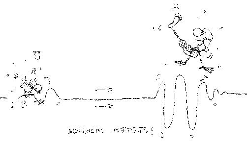
Figure 13. A nice representation of nonlocal effects.

Then, plugging (W.7) into (W.6), we obtain the equation in divergence form which was claimed in (3.7).

Appendix X Proof of (3.12)

First we observe that

(X.1) $$\int_{\mathbb{R}^{n}\setminus B_{1}}\frac{|u(x)-u(x-y)|}{|M(x,y)\,y|^{n+2s}}\,dy\leqslant\,{\rm const}\,\int_{\mathbb{R}^{n}\setminus B_{1}}\frac{dy}{|y|^{n+2s}}\leqslant\frac{\,{\rm const}\,}{s}.$$

Furthermore, for $y\in B_{1}$,

$$M(x,y)\,y=M(x,0)\,y+O(|y|^{2}).$$

Consequently,

$$|M(x,y)\,y|^{2}=|M(x,0)\,y|^{2}+O(|y|^{3})$$

and so, from the non-degeneracy of $M(\cdot,\cdot)$,

$$|M(x,y)\,y|^{-n-2s}=\big{(}|M(x,0)\,y|^{2}+O(|y|^{3})\big{)}^{-\frac{n+2s}{2}}$$

$$\qquad=|M(x,0)\,y|^{-n-2s}\big{(}1+O(|y|)\big{)}^{-\frac{n+2s}{2}}=|M(x,0)\,y|^{-n-2s}\big{(}1-O(|y|)\big{)}.$$

Using this and the expansion in (W.2), we see that, for $y\in B_{1}$,

$$\frac{u(x)-u(x-y)-\nabla u(x)\cdot y}{|M(x,y)\,y|^{n+2s}}$$

$$= |M(x,0)\,y|^{-n-2s}\big{(}1-O(|y|)\big{)}\left(-\frac{1}{2}D^{2}u(x)\,y\cdot y+O(|y|^{3})\right)$$

$$= |M(x,0)\,y|^{-n-2s}\left(-\frac{1}{2}D^{2}u(x)\,y\cdot y+O(|y|^{3})\right).$$

Thus, since, in the light of (3.11), we know that the map $y\mapsto\frac{\nabla u(x)\cdot y}{|M(x,y)\,y|^{n+2s}}$ is odd, we can write that

$$\int_{B_{1}}\frac{u(x)-u(x-y)}{|M(x,y)\,y|^{n+2s}}\,dy = \int_{B_{1}}\frac{u(x)-u(x-y)-\nabla u(x)\cdot y}{|M(x,y)\,y|^{n+2s}}\,dy$$

$$= -\frac{1}{2}\int_{B_{1}}\frac{D^{2}u(x)\,y\cdot y}{|M(x,0)\,y|^{n+2s}}\,dy+\frac{O(1)}{3-2s}$$

$$= -\frac{\,{\rm const}\,}{1-s}\int_{S^{n-1}}\frac{D^{2}u(x)\,\omega\cdot\omega}{|M(x,0)\,\omega|^{n+2s}}\,d{\mathcal{H}}^{n-1}_{\omega}+\frac{O(1)}{3-2s},$$

where the last identity follows by using (W.5) (with $\alpha:=0$). From this and (X.1) we obtain that

$$\lim_{s\nearrow 1}(1-s)\,\int_{\mathbb{R}^{n}}\frac{u(x)-u(x-y)}{|M(x,y)\,y|^{n+2s}}\,dy = \lim_{s\nearrow 1}(1-s)\,\int_{B_{1}}\frac{u(x)-u(x-y)}{|M(x,y)\,y|^{n+2s}}\,dy$$

$$= -\,{\rm const}\,\int_{S^{n-1}}\frac{D^{2}u(x)\,\omega\cdot\omega}{|M(x,0)\,\omega|^{n+2}}\,d{\mathcal{H}}^{n-1}_{\omega}$$

$$= -\,{\rm const}\,\sum_{i,j=1}^{n}\int_{S^{n-1}}\frac{\omega_{i}\omega_{j}}{|M(x,0)\,\omega|^{n+2}}\,d{\mathcal{H}}^{n-1}_{\omega}\,\partial^{2}_{ij}u(x),$$

which gives (3.12).

References

AbatangeloNicolaLarge $s$-harmonic functions and boundary blow-up solutions for the fractional laplacianDiscrete Contin. Dyn. Syst.352015125555–5607ISSN 1078-0947Review MathReviewsDocument@article{MR3393247, author = {Abatangelo, Nicola}, title = {Large $s$-harmonic functions and boundary blow-up solutions for the fractional Laplacian}, journal = {Discrete Contin. Dyn. Syst.}, volume = {35}, date = {2015}, number = {12}, pages = {5555–5607}, issn = {1078-0947}, review = {\MR{3393247}}, doi = {10.3934/dcds.2015.35.5555}} AbatangeloNicolaDupaigneLouisNonhomogeneous boundary conditions for the spectral fractional laplacianAnn. Inst. H. Poincaré Anal. Non Linéaire3420172439–467ISSN 0294-1449Review MathReviewsDocument@article{MR3610940, author = {Abatangelo, Nicola}, author = {Dupaigne, Louis}, title = {Nonhomogeneous boundary conditions for the spectral fractional Laplacian}, journal = {Ann. Inst. H. Poincar\'e Anal. Non Lin\'eaire}, volume = {34}, date = {2017}, number = {2}, pages = {439–467}, issn = {0294-1449}, review = {\MR{3610940}}, doi = {10.1016/j.anihpc.2016.02.001}} AbatangeloNicolaJarohsSvenSaldañaAlbertoPositive powers of the laplacian: from hypersingular integrals to boundary value problemsCommun. Pure Appl. Anal.1720183899–922ISSN 1534-0392Review MathReviewsDocument@article{AJS1, author = {Abatangelo, Nicola}, author = {Jarohs, Sven}, author = {Salda\~{n}a, Alberto}, title = {Positive powers of the Laplacian: from hypersingular integrals to boundary value problems}, journal = {Commun. Pure Appl. Anal.}, volume = {17}, date = {2018}, number = {3}, pages = {899–922}, issn = {1534-0392}, review = {\MR{3809107}}, doi = {10.3934/cpaa.2018045}} AbatangeloNicolaJarohsSvenSaldañaAlbertoGreen function and martin kernel for higher-order fractional laplacians in ballsNonlinear Anal.1752018173–190ISSN 0362-546XReview MathReviewsDocument@article{AJS2, author = {Abatangelo, Nicola}, author = {Jarohs, Sven}, author = {Salda\~{n}a, Alberto}, title = {Green function and Martin kernel for higher-order fractional Laplacians in balls}, journal = {Nonlinear Anal.}, volume = {175}, date = {2018}, pages = {173–190}, issn = {0362-546X}, review = {\MR{3830727}}, doi = {10.1016/j.na.2018.05.019}} AbatangeloNicolaJarohsSvenSaldañaAlbertoOn the loss of maximum principles for higher-order fractional laplaciansProc. Amer. Math. Soc.1462018114823–4835ISSN 0002-9939Review MathReviewsDocument@article{AJS3, author = {Abatangelo, Nicola}, author = {Jarohs, Sven}, author = {Salda\~{n}a, Alberto}, title = {On the loss of maximum principles for higher-order fractional Laplacians}, journal = {Proc. Amer. Math. Soc.}, volume = {146}, date = {2018}, number = {11}, pages = {4823–4835}, issn = {0002-9939}, review = {\MR{3856149}}, doi = {10.1090/proc/14165}} AffiliElisaDipierroSerenaValdinociEnricoDecay estimates in time for classical and anomalous diffusionarXiv e-prints2018arXiv1812.09451math.APhttps://ui.adsabs.harvard.edu/\#abs/2018arXiv181209451AProvided by the SAO/NASA Astrophysics Data System@article{AFFILI, author = {Affili, Elisa}, author = {Dipierro, Serena}, author = {Valdinoci, Enrico}, title = {Decay estimates in time for classical and anomalous diffusion}, journal = {arXiv e-prints}, date = {2018}, archiveprefix = {arXiv}, eprint = {1812.09451}, primaryclass = {math.AP}, adsurl = {https://ui.adsabs.harvard.edu/\#abs/2018arXiv181209451A}, adsnote = {Provided by the SAO/NASA Astrophysics Data System}} AllenMarkCaffarelliLuisVasseurAlexisA parabolic problem with a fractional time derivativeArch. Ration. Mech. Anal.22120162603–630ISSN 0003-9527Review MathReviewsDocument@article{MR3488533, author = {Allen, Mark}, author = {Caffarelli, Luis}, author = {Vasseur, Alexis}, title = {A parabolic problem with a fractional time derivative}, journal = {Arch. Ration. Mech. Anal.}, volume = {221}, date = {2016}, number = {2}, pages = {603–630}, issn = {0003-9527}, review = {\MR{3488533}}, doi = {10.1007/s00205-016-0969-z}} Andreu-VailloFuensantaMazónJosé M.RossiJulio D.Toledo-MeleroJ. JuliánNonlocal diffusion problemsMathematical Surveys and Monographs165American Mathematical Society, Providence, RI; Real Sociedad Matemática Española, Madrid2010xvi+256ISBN 978-0-8218-5230-9Review MathReviewsDocument@book{MR2722295, author = {Andreu-Vaillo, Fuensanta}, author = {Maz\'on, Jos\'e M.}, author = {Rossi, Julio D.}, author = {Toledo-Melero, J. Juli\'an}, title = {Nonlocal diffusion problems}, series = {Mathematical Surveys and Monographs}, volume = {165}, publisher = {American Mathematical Society, Providence, RI; Real Sociedad Matem\'atica Espa\~nola, Madrid}, date = {2010}, pages = {xvi+256}, isbn = {978-0-8218-5230-9}, review = {\MR{2722295}}, doi = {10.1090/surv/165}} ApplebaumDavidLévy processes and stochastic calculusCambridge Studies in Advanced Mathematics1162Cambridge University Press, Cambridge2009xxx+460ISBN 978-0-521-73865-1Review MathReviewsDocument@book{MR2512800, author = {Applebaum, David}, title = {L\'evy processes and stochastic calculus}, series = {Cambridge Studies in Advanced Mathematics}, volume = {116}, edition = {2}, publisher = {Cambridge University Press, Cambridge}, date = {2009}, pages = {xxx+460}, isbn = {978-0-521-73865-1}, review = {\MR{2512800}}, doi = {10.1017/CBO9780511809781}} ArkhincheevV. E.BaskinÉ. M.Anomalous diffusion and drift in a comb model of percolation clustersJ. Exp. Theor. Phys.731991161–165@article{comb, author = {Arkhincheev, V. E.}, author = {Baskin, \'E. M.}, title = {Anomalous diffusion and drift in a comb model of percolation clusters}, journal = {J. Exp. Theor. Phys.}, volume = {73}, date = {1991}, pages = {161–165}} BalakrishnanA. V.Fractional powers of closed operators and the semigroups generated by themPacific J. Math.101960419–437ISSN 0030-8730Review MathReviews@article{MR0115096, author = {Balakrishnan, A. V.}, title = {Fractional powers of closed operators and the semigroups generated by them}, journal = {Pacific J. Math.}, volume = {10}, date = {1960}, pages = {419–437}, issn = {0030-8730}, review = {\MR{0115096}}} BañuelosRodrigoBogdanKrzysztofLévy processes and fourier multipliersJ. Funct. Anal.25020071197–213ISSN 0022-1236Review MathReviewsDocument@article{MR2345912, author = {Ba\~nuelos, Rodrigo}, author = {Bogdan, Krzysztof}, title = {L\'evy processes and Fourier multipliers}, journal = {J. Funct. Anal.}, volume = {250}, date = {2007}, number = {1}, pages = {197–213}, issn = {0022-1236}, review = {\MR{2345912}}, doi = {10.1016/j.jfa.2007.05.013}} BarriosBegoñaPeralIreneoSoriaFernandoValdinociEnricoA widder’s type theorem for the heat equation with nonlocal diffusionArch. Ration. Mech. Anal.21320142629–650ISSN 0003-9527Review MathReviewsDocument@article{MR3211862, author = {Barrios, Bego\~na}, author = {Peral, Ireneo}, author = {Soria, Fernando}, author = {Valdinoci, Enrico}, title = {A Widder's type theorem for the heat equation with nonlocal diffusion}, journal = {Arch. Ration. Mech. Anal.}, volume = {213}, date = {2014}, number = {2}, pages = {629–650}, issn = {0003-9527}, review = {\MR{3211862}}, doi = {10.1007/s00205-014-0733-1}} BassRichard F.LevinDavid A.Harnack inequalities for jump processesPotential Anal.1720024375–388ISSN 0926-2601Review MathReviewsDocument@article{MR1918242, author = {Bass, Richard F.}, author = {Levin, David A.}, title = {Harnack inequalities for jump processes}, journal = {Potential Anal.}, volume = {17}, date = {2002}, number = {4}, pages = {375–388}, issn = {0926-2601}, review = {\MR{1918242}}, doi = {10.1023/A:1016378210944}} BendikovA.Asymptotic formulas for symmetric stable semigroupsExposition. Math.1219944381–384ISSN 0723-0869Review MathReviews@article{MR1297844, author = {Bendikov, A.}, title = {Asymptotic formulas for symmetric stable semigroups}, journal = {Exposition. Math.}, volume = {12}, date = {1994}, number = {4}, pages = {381–384}, issn = {0723-0869}, review = {\MR{1297844}}} BertoinJeanLévy processesCambridge Tracts in Mathematics121Cambridge University Press, Cambridge1996x+265ISBN 0-521-56243-0Review MathReviews@book{MR1406564, author = {Bertoin, Jean}, title = {L\'evy processes}, series = {Cambridge Tracts in Mathematics}, volume = {121}, publisher = {Cambridge University Press, Cambridge}, date = {1996}, pages = {x+265}, isbn = {0-521-56243-0}, review = {\MR{1406564}}} BlumenthalR. M.GetoorR. K.Some theorems on stable processesTrans. Amer. Math. Soc.951960263–273ISSN 0002-9947Review MathReviewsDocument@article{MR0119247, author = {Blumenthal, R. M.}, author = {Getoor, R. K.}, title = {Some theorems on stable processes}, journal = {Trans. Amer. Math. Soc.}, volume = {95}, date = {1960}, pages = {263–273}, issn = {0002-9947}, review = {\MR{0119247}}, doi = {10.2307/1993291}} BogdanKrzysztofByczkowskiTomaszPotential theory for the $\alpha$-stable schrödinger operator on bounded lipschitz domainsStudia Math.1331999153–92ISSN 0039-3223Review MathReviews@article{MR1671973, author = {Bogdan, Krzysztof}, author = {Byczkowski, Tomasz}, title = {Potential theory for the $\alpha$-stable Schr\"odinger operator on bounded Lipschitz domains}, journal = {Studia Math.}, volume = {133}, date = {1999}, number = {1}, pages = {53–92}, issn = {0039-3223}, review = {\MR{1671973}}} BogdanK.ŻakT.On kelvin transformationJ. Theoret. Probab.192006189–120ISSN 0894-9840Review MathReviews@article{MR2256481, author = {Bogdan, K.}, author = {\.Zak, T.}, title = {On Kelvin transformation}, journal = {J. Theoret. Probab.}, volume = {19}, date = {2006}, number = {1}, pages = {89–120}, issn = {0894-9840}, review = {\MR{2256481}}} BonforteMatteoFigalliAlessioVázquezJuan LuisSharp global estimates for local and nonlocal porous medium-type equations in bounded domainsAnal. PDE1120184945–982ISSN 2157-5045Review MathReviewsDocument@article{2016arXiv161009881B, author = {Bonforte, Matteo}, author = {Figalli, Alessio}, author = {V\'{a}zquez, Juan Luis}, title = {Sharp global estimates for local and nonlocal porous medium-type equations in bounded domains}, journal = {Anal. PDE}, volume = {11}, date = {2018}, number = {4}, pages = {945–982}, issn = {2157-5045}, review = {\MR{3749373}}, doi = {10.2140/apde.2018.11.945}} BrascoLorenzoMosconiSunraSquassinaMarcoOptimal decay of extremals for the fractional sobolev inequalityCalc. Var. Partial Differential Equations5520162Paper No. 23, 32ISSN 0944-2669Review MathReviewsDocument@article{MR3461371, author = {Brasco, Lorenzo}, author = {Mosconi, Sunra}, author = {Squassina, Marco}, title = {Optimal decay of extremals for the fractional Sobolev inequality}, journal = {Calc. Var. Partial Differential Equations}, volume = {55}, date = {2016}, number = {2}, pages = {Paper No. 23, 32}, issn = {0944-2669}, review = {\MR{3461371}}, doi = {10.1007/s00526-016-0958-y}} BucurClaudiaSome observations on the green function for the ball in the fractional laplace frameworkCommun. Pure Appl. Anal.1520162657–699ISSN 1534-0392Review MathReviewsDocument@article{MR3461641, author = {Bucur, Claudia}, title = {Some observations on the Green function for the ball in the fractional Laplace framework}, journal = {Commun. Pure Appl. Anal.}, volume = {15}, date = {2016}, number = {2}, pages = {657–699}, issn = {1534-0392}, review = {\MR{3461641}}, doi = {10.3934/cpaa.2016.15.657}} BucurClaudiaLocal density of caputo-stationary functions in the space of smooth functionsESAIM Control Optim. Calc. Var.23201741361–1380ISSN 1292-8119Review MathReviewsDocument@article{ESAIM, author = {Bucur, Claudia}, title = {Local density of Caputo-stationary functions in the space of smooth functions}, journal = {ESAIM Control Optim. Calc. Var.}, volume = {23}, date = {2017}, number = {4}, pages = {1361–1380}, issn = {1292-8119}, review = {\MR{3716924}}, doi = {10.1051/cocv/2016056}} BucurClaudiaLombardiniLucaValdinociEnricoComplete stickiness of nonlocal minimal surfaces for small values of the fractional parameterto appear on Ann. Inst. H. Poincaré Anal. Non LinéaireDocument@article{POICLA, author = {Bucur, Claudia}, author = {Lombardini, Luca}, author = {Valdinoci, Enrico}, title = {Complete stickiness of nonlocal minimal surfaces for small values of the fractional parameter}, journal = {to appear on Ann. Inst. H. Poincar\'e Anal. Non Lin\'eaire}, doi = {10.1016/j.anihpc.2018.08.003}} BucurClaudiaValdinociEnricoNonlocal diffusion and applicationsLecture Notes of the Unione Matematica Italiana20Springer, [Cham]; Unione Matematica Italiana, Bologna2016xii+155ISBN 978-3-319-28738-6ISBN 978-3-319-28739-3Review MathReviewsDocument@book{MR3469920, author = {Bucur, Claudia}, author = {Valdinoci, Enrico}, title = {Nonlocal diffusion and applications}, series = {Lecture Notes of the Unione Matematica Italiana}, volume = {20}, publisher = {Springer, [Cham]; Unione Matematica Italiana, Bologna}, date = {2016}, pages = {xii+155}, isbn = {978-3-319-28738-6}, isbn = {978-3-319-28739-3}, review = {\MR{3469920}}, doi = {10.1007/978-3-319-28739-3}} CabréXavierCozziMatteoA gradient estimate for nonlocal minimal graphsto appear on Duke Math. J.@article{DUCA, author = {Cabr\'e, Xavier}, author = {Cozzi, Matteo}, title = {A gradient estimate for nonlocal minimal graphs}, journal = {to appear on Duke Math. J.}} CabréXavierSireYannickNonlinear equations for fractional laplacians ii: existence, uniqueness, and qualitative properties of solutionsTrans. Amer. Math. Soc.36720152911–941ISSN 0002-9947Review MathReviewsDocument@article{MR3280032, author = {Cabr\'e, Xavier}, author = {Sire, Yannick}, title = {Nonlinear equations for fractional Laplacians II: Existence, uniqueness, and qualitative properties of solutions}, journal = {Trans. Amer. Math. Soc.}, volume = {367}, date = {2015}, number = {2}, pages = {911–941}, issn = {0002-9947}, review = {\MR{3280032}}, doi = {10.1090/S0002-9947-2014-05906-0}} CaffarelliL. A.Further regularity for the signorini problemComm. Partial Differential Equations4197991067–1075ISSN 0360-5302Review MathReviewsDocument@article{MR542512, author = {Caffarelli, L. A.}, title = {Further regularity for the Signorini problem}, journal = {Comm. Partial Differential Equations}, volume = {4}, date = {1979}, number = {9}, pages = {1067–1075}, issn = {0360-5302}, review = {\MR{542512}}, doi = {10.1080/03605307908820119}} CaffarelliLuisCharroFernandoOn a fractional monge-ampère operatorAnn. PDE120151Art. 4, 47ISSN 2199-2576Review MathReviews@article{MR3479063, author = {Caffarelli, Luis}, author = {Charro, Fernando}, title = {On a fractional Monge-Amp\`ere operator}, journal = {Ann. PDE}, volume = {1}, date = {2015}, number = {1}, pages = {Art. 4, 47}, issn = {2199-2576}, review = {\MR{3479063}}} CaffarelliLuisSilvestreLuisAn extension problem related to the fractional laplacianComm. Partial Differential Equations3220077-91245–1260ISSN 0360-5302Review MathReviewsDocument@article{MR2354493, author = {Caffarelli, Luis}, author = {Silvestre, Luis}, title = {An extension problem related to the fractional Laplacian}, journal = {Comm. Partial Differential Equations}, volume = {32}, date = {2007}, number = {7-9}, pages = {1245–1260}, issn = {0360-5302}, review = {\MR{2354493}}, doi = {10.1080/03605300600987306}} CaffarelliLuisSilvestreLuisRegularity theory for fully nonlinear integro-differential equationsComm. Pure Appl. Math.6220095597–638ISSN 0010-3640Review MathReviews@article{MR2494809, author = {Caffarelli, Luis}, author = {Silvestre, Luis}, title = {Regularity theory for fully nonlinear integro-differential equations}, journal = {Comm. Pure Appl. Math.}, volume = {62}, date = {2009}, number = {5}, pages = {597–638}, issn = {0010-3640}, review = {\MR{2494809}}} CaffarelliLuisSilvestreLuisHölder regularity for generalized master equations with rough kernelstitle={Advances in analysis: the legacy of Elias M. Stein}, series={Princeton Math. Ser.}, volume={50}, publisher={Princeton Univ. Press, Princeton, NJ}, 201463–83Review MathReviews@article{MR3329847, author = {Caffarelli, Luis}, author = {Silvestre, Luis}, title = {H\"older regularity for generalized master equations with rough kernels}, conference = {title={Advances in analysis: the legacy of Elias M. Stein}, }, book = {series={Princeton Math. Ser.}, volume={50}, publisher={Princeton Univ. Press, Princeton, NJ}, }, date = {2014}, pages = {63–83}, review = {\MR{3329847}}} CaffarelliLuisSoriaFernandoVázquezJuan LuisRegularity of solutions of the fractional porous medium flowJ. Eur. Math. Soc. (JEMS)15201351701–1746ISSN 1435-9855Review MathReviewsDocument@article{MR3082241, author = {Caffarelli, Luis}, author = {Soria, Fernando}, author = {V\'azquez, Juan Luis}, title = {Regularity of solutions of the fractional porous medium flow}, journal = {J. Eur. Math. Soc. (JEMS)}, volume = {15}, date = {2013}, number = {5}, pages = {1701–1746}, issn = {1435-9855}, review = {\MR{3082241}}, doi = {10.4171/JEMS/401}} CaffarelliLuis A.VázquezJuan LuisAsymptotic behaviour of a porous medium equation with fractional diffusionDiscrete Contin. Dyn. Syst.29201141393–1404ISSN 1078-0947Review MathReviews@article{MR2773189, author = {Caffarelli, Luis A.}, author = {V\'azquez, Juan Luis}, title = {Asymptotic behaviour of a porous medium equation with fractional diffusion}, journal = {Discrete Contin. Dyn. Syst.}, volume = {29}, date = {2011}, number = {4}, pages = {1393–1404}, issn = {1078-0947}, review = {\MR{2773189}}} CaputoMicheleLinear models of dissipation whose $Q$ is almost frequency independent. iiReprinted from Geophys. J. R. Astr. Soc. 13 (1967), no. 5, 529–539Fract. Calc. Appl. Anal.11200814–14ISSN 1311-0454Review MathReviews@article{MR2379269, author = {Caputo, Michele}, title = {Linear models of dissipation whose $Q$ is almost frequency independent. II}, note = {Reprinted from Geophys. J. R. Astr. Soc. {\bf 13} (1967), no. 5, 529–539}, journal = {Fract. Calc. Appl. Anal.}, volume = {11}, date = {2008}, number = {1}, pages = {4–14}, issn = {1311-0454}, review = {\MR{2379269}}} CarbottiAlessandroDipierroSerenaValdinociEnricoLocal density of caputo-stationary functions of any orderto appear on Complex Var. Elliptic Equ.Document@article{2018arXiv180904005C, author = {{Carbotti}, Alessandro}, author = {{Dipierro}, Serena}, author = {{Valdinoci}, Enrico}, title = {Local density of Caputo-stationary functions of any order}, journal = {to appear on Complex Var. Elliptic Equ.}, doi = {10.1080/17476933.2018.1544631}} CarbottiAlessandroDipierroSerenaValdinociEnricoLocal Density of Solutions to Fractional Equations series=Graduate Studies in MathematicsDe Gruyter, Berlin2019@book{2018arXiv181008448C, author = {{Carbotti}, Alessandro}, author = {{Dipierro}, Serena}, author = {{Valdinoci}, Enrico}, title = {{Local Density of Solutions to Fractional Equations} series={Graduate Studies in Mathematics}}, publisher = {De Gruyter, Berlin}, date = {2019}} CarmonaRenéMastersWen ChenSimonBarryRelativistic schrödinger operators: asymptotic behavior of the eigenfunctionsJ. Funct. Anal.9119901117–142ISSN 0022-1236Review MathReviewsDocument@article{MR1054115, author = {Carmona, Ren\'e}, author = {Masters, Wen Chen}, author = {Simon, Barry}, title = {Relativistic Schr\"odinger operators: asymptotic behavior of the eigenfunctions}, journal = {J. Funct. Anal.}, volume = {91}, date = {1990}, number = {1}, pages = {117–142}, issn = {0022-1236}, review = {\MR{1054115}}, doi = {10.1016/0022-1236(90)90049-Q}} CesaroniAnnalisaNovagaMatteoSymmetric self-shrinkers for the fractional mean curvature flowArXiv e-prints2018arXiv1812.01847math.APhttps://ui.adsabs.harvard.edu/\#abs/2018arXiv181201847CProvided by the SAO/NASA Astrophysics Data System@article{2018arXiv181201847C, author = {{Cesaroni}, Annalisa}, author = {{Novaga}, Matteo}, title = {Symmetric self-shrinkers for the fractional mean curvature flow}, journal = {ArXiv e-prints}, date = {2018}, archiveprefix = {arXiv}, eprint = {1812.01847}, primaryclass = {math.AP}, adsurl = {https://ui.adsabs.harvard.edu/\#abs/2018arXiv181201847C}, adsnote = {Provided by the SAO/NASA Astrophysics Data System}} CesaroniAnnalisaDipierroSerenaNovagaMatteoValdinociEnricoFattening and nonfattening phenomena for planar nonlocal curvature flowsto appear on Math. Ann.Document@article{FATTE, author = {{Cesaroni}, Annalisa}, author = {Dipierro, Serena}, author = {{Novaga}, Matteo}, author = {Valdinoci, Enrico}, title = {Fattening and nonfattening phenomena for planar nonlocal curvature flows}, journal = {to appear on Math. Ann.}, doi = {10.1007/s00208-018-1793-6}} Chang LaraHéctorDávilaGonzaloRegularity for solutions of non local parabolic equationsCalc. Var. Partial Differential Equations4920141-2139–172ISSN 0944-2669Review MathReviewsDocument@article{MR3148110, author = {Chang Lara, H\'ector}, author = {D\'avila, Gonzalo}, title = {Regularity for solutions of non local parabolic equations}, journal = {Calc. Var. Partial Differential Equations}, volume = {49}, date = {2014}, number = {1-2}, pages = {139–172}, issn = {0944-2669}, review = {\MR{3148110}}, doi = {10.1007/s00526-012-0576-2}} CintiEleonoraSerraJoaquimValdinociEnricoQuantitative flatness results and $BV$-estimates for stable nonlocal minimal surfacesto appear on J. Differential Geom.@article{BVSUP, author = {Cinti, Eleonora}, author = {Serra, Joaquim}, author = {Valdinoci, Enrico}, title = {Quantitative flatness results and $BV$-estimates for stable nonlocal minimal surfaces}, journal = {to appear on J. Differential Geom.}} CintiEleonoraSinestrariCarloValdinociEnricoNeckpinch singularities in fractional mean curvature flowsProc. Amer. Math. Soc.146201862637–2646ISSN 0002-9939Review MathReviewsDocument@article{SIN, author = {Cinti, Eleonora}, author = {Sinestrari, Carlo}, author = {Valdinoci, Enrico}, title = {Neckpinch singularities in fractional mean curvature flows}, journal = {Proc. Amer. Math. Soc.}, volume = {146}, date = {2018}, number = {6}, pages = {2637–2646}, issn = {0002-9939}, review = {\MR{3778164}}, doi = {10.1090/proc/14002}} CovilleJérômeHarnack type inequality for positive solution of some integral equationAnn. Mat. Pura Appl. (4)19120123503–528ISSN 0373-3114Review MathReviewsDocument@article{MR2958346, author = {Coville, J\'er\^ome}, title = {Harnack type inequality for positive solution of some integral equation}, journal = {Ann. Mat. Pura Appl. (4)}, volume = {191}, date = {2012}, number = {3}, pages = {503–528}, issn = {0373-3114}, review = {\MR{2958346}}, doi = {10.1007/s10231-011-0193-2}} CoxJohn C.The valuation of options for alternative stochastic processesJ. Finan. Econ.319761-2145–166Document@article{COX, author = {Cox, John C.}, title = {The valuation of options for alternative stochastic processes}, journal = {J. Finan. Econ.}, volume = {3}, date = {1976}, number = {1-2}, pages = {145–166}, doi = {10.1016/0304-405X(76)90023-4}} CozziMatteoValdinociEnricoOn the growth of nonlocal catenoidsto appear on Atti Accad. Naz. Lincei Rend. Lincei Mat. Appl.@article{2018arXiv181112141C, author = {{Cozzi}, Matteo}, author = {{Valdinoci}, Enrico}, title = {On the growth of nonlocal catenoids}, journal = {to appear on Atti Accad. Naz. Lincei Rend. Lincei Mat. Appl.}} DávilaJuandel PinoManuelWeiJunchengNonlocal $s$-minimal surfaces and lawson conesJ. Differential Geom.10920181111–175ISSN 0022-040XReview MathReviewsDocument@article{LAWSON, author = {D\'{a}vila, Juan}, author = {del Pino, Manuel}, author = {Wei, Juncheng}, title = {Nonlocal $s$-minimal surfaces and Lawson cones}, journal = {J. Differential Geom.}, volume = {109}, date = {2018}, number = {1}, pages = {111–175}, issn = {0022-040X}, review = {\MR{3798717}}, doi = {10.4310/jdg/1525399218}} DengC.-S.SchillingR. L.Exact asymptotic formulas for the heat kernels of space and time-fractional equationsArXiv e-printsarXiv1803.11435math.PR2018http://adsabs.harvard.edu/abs/2018arXiv180311435DProvided by the SAO/NASA Astrophysics Data System@article{2018arXiv180311435D, author = {Deng, C.-S.}, author = {Schilling, R.~L.}, title = {Exact Asymptotic Formulas for the Heat Kernels of Space and Time-Fractional Equations}, journal = {ArXiv e-prints}, archiveprefix = {arXiv}, eprint = {1803.11435}, primaryclass = {math.PR}, date = {2018}, adsurl = {http://adsabs.harvard.edu/abs/2018arXiv180311435D}, adsnote = {Provided by the SAO/NASA Astrophysics Data System}} de PabloArturoQuirósFernandoRodríguezAnaVázquezJuan LuisA fractional porous medium equationAdv. Math.226201121378–1409ISSN 0001-8708Review MathReviewsDocument@article{MR2737788, author = {de Pablo, Arturo}, author = {Quir\'os, Fernando}, author = {Rodr\'\i guez, Ana}, author = {V\'azquez, Juan Luis}, title = {A fractional porous medium equation}, journal = {Adv. Math.}, volume = {226}, date = {2011}, number = {2}, pages = {1378–1409}, issn = {0001-8708}, review = {\MR{2737788}}, doi = {10.1016/j.aim.2010.07.017}} Di NezzaEleonoraPalatucciGiampieroValdinociEnricoHitchhiker’s guide to the fractional sobolev spacesBull. Sci. Math.13620125521–573ISSN 0007-4497Review MathReviewsDocument@article{MR2944369, author = {Di Nezza, Eleonora}, author = {Palatucci, Giampiero}, author = {Valdinoci, Enrico}, title = {Hitchhiker's guide to the fractional Sobolev spaces}, journal = {Bull. Sci. Math.}, volume = {136}, date = {2012}, number = {5}, pages = {521–573}, issn = {0007-4497}, review = {\MR{2944369}}, doi = {10.1016/j.bulsci.2011.12.004}} DipierroSerenaGrunauHans-ChristophBoggio’s formula for fractional polyharmonic dirichlet problemsAnn. Mat. Pura Appl. (4)196201741327–1344ISSN 0373-3114Review MathReviewsDocument@article{GD, author = {Dipierro, Serena}, author = {Grunau, Hans-Christoph}, title = {Boggio's formula for fractional polyharmonic Dirichlet problems}, journal = {Ann. Mat. Pura Appl. (4)}, volume = {196}, date = {2017}, number = {4}, pages = {1327–1344}, issn = {0373-3114}, review = {\MR{3673669}}, doi = {10.1007/s10231-016-0618-z}} DipierroSerenaPalatucciGiampieroValdinociEnricoDislocation dynamics in crystals: a macroscopic theory in a fractional laplace settingComm. Math. Phys.333201521061–1105ISSN 0010-3616Review MathReviewsDocument@article{MR3296170, author = {Dipierro, Serena}, author = {Palatucci, Giampiero}, author = {Valdinoci, Enrico}, title = {Dislocation dynamics in crystals: a macroscopic theory in a fractional Laplace setting}, journal = {Comm. Math. Phys.}, volume = {333}, date = {2015}, number = {2}, pages = {1061–1105}, issn = {0010-3616}, review = {\MR{3296170}}, doi = {10.1007/s00220-014-2118-6}} DipierroSerenaRos-OtonXavierValdinociEnricoNonlocal problems with neumann boundary conditionsRev. Mat. Iberoam.3320172377–416ISSN 0213-2230Review MathReviewsDocument@article{MR3651008, author = {Dipierro, Serena}, author = {Ros-Oton, Xavier}, author = {Valdinoci, Enrico}, title = {Nonlocal problems with Neumann boundary conditions}, journal = {Rev. Mat. Iberoam.}, volume = {33}, date = {2017}, number = {2}, pages = {377–416}, issn = {0213-2230}, review = {\MR{3651008}}, doi = {10.4171/RMI/942}} DipierroSerenaSavinOvidiuValdinociEnricoGraph properties for nonlocal minimal surfacesCalc. Var. Partial Differential Equations5520164Paper No. 86, 25ISSN 0944-2669Review MathReviewsDocument@article{MR3516886, author = {Dipierro, Serena}, author = {Savin, Ovidiu}, author = {Valdinoci, Enrico}, title = {Graph properties for nonlocal minimal surfaces}, journal = {Calc. Var. Partial Differential Equations}, volume = {55}, date = {2016}, number = {4}, pages = {Paper No. 86, 25}, issn = {0944-2669}, review = {\MR{3516886}}, doi = {10.1007/s00526-016-1020-9}} DipierroSerenaSavinOvidiuValdinociEnricoAll functions are locally $s$-harmonic up to a small errorJ. Eur. Math. Soc. (JEMS)1920174957–966ISSN 1435-9855Review MathReviewsDocument@article{MR3626547, author = {Dipierro, Serena}, author = {Savin, Ovidiu}, author = {Valdinoci, Enrico}, title = {All functions are locally $s$-harmonic up to a small error}, journal = {J. Eur. Math. Soc. (JEMS)}, volume = {19}, date = {2017}, number = {4}, pages = {957–966}, issn = {1435-9855}, review = {\MR{3626547}}, doi = {10.4171/JEMS/684}} DipierroSerenaSavinOvidiuValdinociEnricoBoundary behavior of nonlocal minimal surfacesJ. Funct. Anal.272201751791–1851ISSN 0022-1236Review MathReviewsDocument@article{MR3596708, author = {Dipierro, Serena}, author = {Savin, Ovidiu}, author = {Valdinoci, Enrico}, title = {Boundary behavior of nonlocal minimal surfaces}, journal = {J. Funct. Anal.}, volume = {272}, date = {2017}, number = {5}, pages = {1791–1851}, issn = {0022-1236}, review = {\MR{3596708}}, doi = {10.1016/j.jfa.2016.11.016}} DipierroSerenaSavinOvidiuValdinociEnricoLocal approximation of arbitrary functions by solutions of nonlocal equationsto appear on J. Geom. Anal.Document@article{SCALOR, author = {Dipierro, Serena}, author = {Savin, Ovidiu}, author = {Valdinoci, Enrico}, title = {Local approximation of arbitrary functions by solutions of nonlocal equations}, journal = {to appear on J. Geom. Anal.}, doi = {10.1007/s12220-018-0045-z}} DipierroSerenaSavinOvidiuValdinociEnricoDefinition of fractional laplacian for functions with polynomial growthto appear on Rev. Mat. Iberoam.@article{POLYN, author = {Dipierro, Serena}, author = {Savin, Ovidiu}, author = {Valdinoci, Enrico}, title = {Definition of fractional Laplacian for functions with polynomial growth}, journal = {to appear on Rev. Mat. Iberoam.}} DipierroSerenaSerraJoaquimValdinociEnricoImprovement of flatness for nonlocal phase transitionsto appear on Amer. J. Math.@article{owduir375957973, author = {Dipierro, Serena}, author = {Serra, Joaquim}, author = {Valdinoci, Enrico}, title = {Improvement of flatness for nonlocal phase transitions}, journal = {to appear on Amer. J. Math.}} DipierroSerenaSoaveNicolaValdinociEnricoOn stable solutions of boundary reaction-diffusion equations and applications to nonlocal problems with neumann dataIndiana Univ. Math. J.6720181429–469ISSN 0022-2518Review MathReviewsDocument@article{SOA, author = {Dipierro, Serena}, author = {Soave, Nicola}, author = {Valdinoci, Enrico}, title = {On stable solutions of boundary reaction-diffusion equations and applications to nonlocal problems with Neumann data}, journal = {Indiana Univ. Math. J.}, volume = {67}, date = {2018}, number = {1}, pages = {429–469}, issn = {0022-2518}, review = {\MR{3776028}}, doi = {10.1512/iumj.2018.67.6282}} DipierroSerenaValdinociEnricoA simple mathematical model inspired by the purkinje cells: from delayed travelling waves to fractional diffusionBull. Math. Biol.80201871849–1870ISSN 0092-8240Review MathReviewsDocument@article{PuPOw2e3we, author = {Dipierro, Serena}, author = {Valdinoci, Enrico}, title = {A simple mathematical model inspired by the Purkinje cells: from delayed travelling waves to fractional diffusion}, journal = {Bull. Math. Biol.}, volume = {80}, date = {2018}, number = {7}, pages = {1849–1870}, issn = {0092-8240}, review = {\MR{3814763}}, doi = {10.1007/s11538-018-0437-z}} DydaBartłomiejFractional calculus for power functions and eigenvalues of the fractional laplacianFract. Calc. Appl. Anal.1520124536–555ISSN 1311-0454Review MathReviewsDocument@article{MR2974318, author = {Dyda, Bart\l omiej}, title = {Fractional calculus for power functions and eigenvalues of the fractional Laplacian}, journal = {Fract. Calc. Appl. Anal.}, volume = {15}, date = {2012}, number = {4}, pages = {536–555}, issn = {1311-0454}, review = {\MR{2974318}}, doi = {10.2478/s13540-012-0038-8}} EvansLawrence C.Partial differential equationsGraduate Studies in Mathematics19American Mathematical Society, Providence, RI1998xviii+662ISBN 0-8218-0772-2Review MathReviews@book{MR1625845, author = {Evans, Lawrence C.}, title = {Partial differential equations}, series = {Graduate Studies in Mathematics}, volume = {19}, publisher = {American Mathematical Society, Providence, RI}, date = {1998}, pages = {xviii+662}, isbn = {0-8218-0772-2}, review = {\MR{1625845}}} FallMouhamed MoustaphaWethTobiasNonexistence results for a class of fractional elliptic boundary value problemsJ. Funct. Anal.263201282205–2227ISSN 0022-1236Review MathReviewsDocument@article{MR2964681, author = {Fall, Mouhamed Moustapha}, author = {Weth, Tobias}, title = {Nonexistence results for a class of fractional elliptic boundary value problems}, journal = {J. Funct. Anal.}, volume = {263}, date = {2012}, number = {8}, pages = {2205–2227}, issn = {0022-1236}, review = {\MR{2964681}}, doi = {10.1016/j.jfa.2012.06.018}} FallMouhamed MoustaphaWethTobiasLiouville theorems for a general class of nonlocal operatorsPotential Anal.4520161187–200ISSN 0926-2601Review MathReviewsDocument@article{MR3511811, author = {Fall, Mouhamed Moustapha}, author = {Weth, Tobias}, title = {Liouville theorems for a general class of nonlocal operators}, journal = {Potential Anal.}, volume = {45}, date = {2016}, number = {1}, pages = {187–200}, issn = {0926-2601}, review = {\MR{3511811}}, doi = {10.1007/s11118-016-9546-1}} FarinaAlbertoValdinociEnricoThe state of the art for a conjecture of de giorgi and related problemstitle={Recent progress on reaction-diffusion systems and viscosity solutions}, publisher={World Sci. Publ., Hackensack, NJ}, 200974–96Review MathReviewsDocument@article{MR2528756, author = {Farina, Alberto}, author = {Valdinoci, Enrico}, title = {The state of the art for a conjecture of De Giorgi and related problems}, conference = {title={Recent progress on reaction-diffusion systems and viscosity solutions}, }, book = {publisher={World Sci. Publ., Hackensack, NJ}, }, date = {2009}, pages = {74–96}, review = {\MR{2528756}}, doi = {10.1142/9789812834744\_0004}} FelmerPatricioQuaasAlexanderBoundary blow up solutions for fractional elliptic equationsAsymptot. Anal.7820123123–144ISSN 0921-7134Review MathReviews@article{MR2985500, author = {Felmer, Patricio}, author = {Quaas, Alexander}, title = {Boundary blow up solutions for fractional elliptic equations}, journal = {Asymptot. Anal.}, volume = {78}, date = {2012}, number = {3}, pages = {123–144}, issn = {0921-7134}, review = {\MR{2985500}}} FigalliAlessioSerraJoaquimOn stable solutions for boundary reactions: a de giorgi-type result in dimension $4+1$submitted, preprint at arXiv:1705.027812017@article{FOFISEA, author = {{Figalli}, Alessio}, author = {Serra, Joaquim}, title = {On stable solutions for boundary reactions: a De Giorgi-type result in dimension $4+1$}, journal = {submitted, preprint at arXiv:1705.02781}, date = {2017}} FrankRupert L.LenzmannEnnoSilvestreLuisUniqueness of radial solutions for the fractional laplacianComm. Pure Appl. Math.69201691671–1726ISSN 0010-3640Review MathReviewsDocument@article{MR3530361, author = {Frank, Rupert L.}, author = {Lenzmann, Enno}, author = {Silvestre, Luis}, title = {Uniqueness of radial solutions for the fractional Laplacian}, journal = {Comm. Pure Appl. Math.}, volume = {69}, date = {2016}, number = {9}, pages = {1671–1726}, issn = {0010-3640}, review = {\MR{3530361}}, doi = {10.1002/cpa.21591}} GetoorR. K.First passage times for symmetric stable processes in spaceTrans. Amer. Math. Soc.101196175–90ISSN 0002-9947Review MathReviewsDocument@article{MR0137148, author = {Getoor, R. K.}, title = {First passage times for symmetric stable processes in space}, journal = {Trans. Amer. Math. Soc.}, volume = {101}, date = {1961}, pages = {75–90}, issn = {0002-9947}, review = {\MR{0137148}}, doi = {10.2307/1993412}} GhoshT.SaloM.UhlmannG.The calderón problem for the fractional schrödinger equationArXiv e-printsarXiv1609.09248math.AP2016http://adsabs.harvard.edu/abs/2016arXiv160909248GProvided by the SAO/NASA Astrophysics Data System@article{SALO1, author = {{Ghosh}, T.}, author = {{Salo}, M.}, author = {{Uhlmann}, G.}, title = {The Calder\'on problem for the fractional Schr\"odinger equation}, journal = {ArXiv e-prints}, archiveprefix = {arXiv}, eprint = {1609.09248}, primaryclass = {math.AP}, date = {2016}, adsurl = {http://adsabs.harvard.edu/abs/2016arXiv160909248G}, adsnote = {Provided by the SAO/NASA Astrophysics Data System}} GilbargDavidTrudingerNeil S.Elliptic partial differential equations of second orderClassics in MathematicsReprint of the 1998 editionSpringer-Verlag, Berlin2001xiv+517ISBN 3-540-41160-7Review MathReviews@book{MR1814364, author = {Gilbarg, David}, author = {Trudinger, Neil S.}, title = {Elliptic partial differential equations of second order}, series = {Classics in Mathematics}, note = {Reprint of the 1998 edition}, publisher = {Springer-Verlag, Berlin}, date = {2001}, pages = {xiv+517}, isbn = {3-540-41160-7}, review = {\MR{1814364}}} GiustiEnricoDirect methods in the calculus of variationsWorld Scientific Publishing Co., Inc., River Edge, NJ2003viii+403ISBN 981-238-043-4Review MathReviewsDocument@book{MR1962933, author = {Giusti, Enrico}, title = {Direct methods in the calculus of variations}, publisher = {World Scientific Publishing Co., Inc., River Edge, NJ}, date = {2003}, pages = {viii+403}, isbn = {981-238-043-4}, review = {\MR{1962933}}, doi = {10.1142/9789812795557}} HanQingLinFanghuaElliptic partial differential equationsCourant Lecture Notes in Mathematics12Courant Institute of Mathematical Sciences, New York; American Mathematical Society, Providence, RI2011x+147ISBN 978-0-8218-5313-9Review MathReviews@book{MR2777537, author = {Han, Qing}, author = {Lin, Fanghua}, title = {Elliptic partial differential equations}, series = {Courant Lecture Notes in Mathematics}, volume = {1}, edition = {2}, publisher = {Courant Institute of Mathematical Sciences, New York; American Mathematical Society, Providence, RI}, date = {2011}, pages = {x+147}, isbn = {978-0-8218-5313-9}, review = {\MR{2777537}}} JacobNielsPseudo-differential operators and markov processesMathematical Research94Akademie Verlag, Berlin1996207ISBN 3-05-501731-5Review MathReviews@book{MR1409607, author = {Jacob, Niels}, title = {Pseudo-differential operators and Markov processes}, series = {Mathematical Research}, volume = {94}, publisher = {Akademie Verlag, Berlin}, date = {1996}, pages = {207}, isbn = {3-05-501731-5}, review = {\MR{1409607}}} KaßmannMoritzHarnack-ungleichungen für nichtlokale differentialoperatoren und dirichlet-formenGermanBonner Mathematische Schriften [Bonn Mathematical Publications]336Dissertation, Rheinische Friedrich-Wilhelms-Universität Bonn, Bonn, 2000Universität Bonn, Mathematisches Institut, Bonn2001vi+91Review MathReviews@book{MR1941020, author = {Ka\ss mann, Moritz}, title = {Harnack-Ungleichungen f\"ur nichtlokale Differentialoperatoren und Dirichlet-Formen}, language = {German}, series = {Bonner Mathematische Schriften [Bonn Mathematical Publications]}, volume = {336}, note = {Dissertation, Rheinische Friedrich-Wilhelms-Universit\"at Bonn, Bonn, 2000}, publisher = {Universit\"at Bonn, Mathematisches Institut, Bonn}, date = {2001}, pages = {vi+91}, review = {\MR{1941020}}} KaßmannMoritzA new formulation of harnack’s inequality for nonlocal operatorsEnglish, with English and French summariesC. R. Math. Acad. Sci. Paris349201111-12637–640ISSN 1631-073XReview MathReviewsDocument@article{MR2817382, author = {Ka\ss mann, Moritz}, title = {A new formulation of Harnack's inequality for nonlocal operators}, language = {English, with English and French summaries}, journal = {C. R. Math. Acad. Sci. Paris}, volume = {349}, date = {2011}, number = {11-12}, pages = {637–640}, issn = {1631-073X}, review = {\MR{2817382}}, doi = {10.1016/j.crma.2011.04.014}} KaßmannMoritzJump processes and nonlocal operatorstitle={Recent developments in nonlocal theory}, publisher={De Gruyter, Berlin}, 2018274–302Review MathReviews@article{K201717, author = {Ka\ss mann, Moritz}, title = {Jump processes and nonlocal operators}, conference = {title={Recent developments in nonlocal theory}, }, book = {publisher={De Gruyter, Berlin}, }, date = {2018}, pages = {274–302}, review = {\MR{3824215}}} KolokoltsovVassiliSymmetric stable laws and stable-like jump-diffusionsProc. London Math. Soc. (3)8020003725–768ISSN 0024-6115Review MathReviewsDocument@article{MR1744782, author = {Kolokoltsov, Vassili}, title = {Symmetric stable laws and stable-like jump-diffusions}, journal = {Proc. London Math. Soc. (3)}, volume = {80}, date = {2000}, number = {3}, pages = {725–768}, issn = {0024-6115}, review = {\MR{1744782}}, doi = {10.1112/S0024611500012314}} KrylovN. V.On the paper “all functions are locally $s$-harmonic up to a small error” by dipierro, savin, and valdinociArXiv e-prints2018arXiv1810.07648math.APhttps://ui.adsabs.harvard.edu/\#abs/2018arXiv181007648KProvided by the SAO/NASA Astrophysics Data System@article{2018arXiv181007648K, author = {{Krylov}, N.~V.}, title = {On the paper ``All functions are locally $s$-harmonic up to a small error'' by Dipierro, Savin, and Valdinoci}, journal = {ArXiv e-prints}, date = {2018}, archiveprefix = {arXiv}, eprint = {1810.07648}, primaryclass = {math.AP}, adsurl = {https://ui.adsabs.harvard.edu/\#abs/2018arXiv181007648K}, adsnote = {Provided by the SAO/NASA Astrophysics Data System}} KuusiTuomoMingioneGiuseppeSireYannickNonlocal equations with measure dataComm. Math. Phys.337201531317–1368ISSN 0010-3616Review MathReviewsDocument@article{MR3339179, author = {Kuusi, Tuomo}, author = {Mingione, Giuseppe}, author = {Sire, Yannick}, title = {Nonlocal equations with measure data}, journal = {Comm. Math. Phys.}, volume = {337}, date = {2015}, number = {3}, pages = {1317–1368}, issn = {0010-3616}, review = {\MR{3339179}}, doi = {10.1007/s00220-015-2356-2}} KwaśnickiMateuszTen equivalent definitions of the fractional laplace operatorFract. Calc. Appl. Anal.20201717–51ISSN 1311-0454Review MathReviewsDocument@article{MR3613319, author = {Kwa\'snicki, Mateusz}, title = {Ten equivalent definitions of the fractional Laplace operator}, journal = {Fract. Calc. Appl. Anal.}, volume = {20}, date = {2017}, number = {1}, pages = {7–51}, issn = {1311-0454}, review = {\MR{3613319}}, doi = {10.1515/fca-2017-0002}} LandkofN. S.Foundations of modern potential theoryTranslated from the Russian by A. P. Doohovskoy; Die Grundlehren der mathematischen Wissenschaften, Band 180Springer-Verlag, New York-Heidelberg1972x+424Review MathReviews@book{MR0350027, author = {Landkof, N. S.}, title = {Foundations of modern potential theory}, note = {Translated from the Russian by A. P. Doohovskoy; Die Grundlehren der mathematischen Wissenschaften, Band 180}, publisher = {Springer-Verlag, New York-Heidelberg}, date = {1972}, pages = {x+424}, review = {\MR{0350027}}} MainardiFrancescoFractional calculus and waves in linear viscoelasticityAn introduction to mathematical modelsImperial College Press, London2010xx+347ISBN 978-1-84816-329-4ISBN 1-84816-329-0Review MathReviewsDocument@book{MR2676137, author = {Mainardi, Francesco}, title = {Fractional calculus and waves in linear viscoelasticity}, note = {An introduction to mathematical models}, publisher = {Imperial College Press, London}, date = {2010}, pages = {xx+347}, isbn = {978-1-84816-329-4}, isbn = {1-84816-329-0}, review = {\MR{2676137}}, doi = {10.1142/9781848163300}} MainardiFrancescoLuchkoYuriPagniniGianniThe fundamental solution of the space-time fractional diffusion equationFract. Calc. Appl. Anal.420012153–192ISSN 1311-0454Review MathReviews@article{MR1829592, author = {Mainardi, Francesco}, author = {Luchko, Yuri}, author = {Pagnini, Gianni}, title = {The fundamental solution of the space-time fractional diffusion equation}, journal = {Fract. Calc. Appl. Anal.}, volume = {4}, date = {2001}, number = {2}, pages = {153–192}, issn = {1311-0454}, review = {\MR{1829592}}} MainardiFrancescoParadisiPaoloGorenfloRudolfProbability distributions generated by fractional diffusion equationssubmitted, preprint at arXiv:0704.0320v12007@article{iqo0eiKAL, author = {Mainardi, Francesco}, author = {Paradisi, Paolo}, author = {Gorenflo, Rudolf}, title = {Probability distributions generated by fractional diffusion equations}, journal = {submitted, preprint at arXiv:0704.0320v1}, date = {2007}} MandelbrotBenoîtThe variation of certain speculative prices1963The Journal of Business36Link@article{MANDEL, author = {Mandelbrot, Beno\^\i t}, title = {The Variation of Certain Speculative Prices}, year = {1963}, journal = {The Journal of Business}, volume = {36}, url = {http://EconPapers.repec.org/RePEc:ucp:jnlbus:v:36:y:1963:p:394}} MazónJose ManuelRossiJulio D.ToledoJuliánThe heat content for nonlocal diffusion with non-singular kernelsAdv. Nonlinear Stud.1720172255–268ISSN 1536-1365Review MathReviewsDocument@article{MR3641640, author = {Maz\'on, Jose Manuel}, author = {Rossi, Julio D.}, author = {Toledo, Juli\'an}, title = {The Heat Content for Nonlocal Diffusion with Non-singular Kernels}, journal = {Adv. Nonlinear Stud.}, volume = {17}, date = {2017}, number = {2}, pages = {255–268}, issn = {1536-1365}, review = {\MR{3641640}}, doi = {10.1515/ans-2017-0005}} MetzlerRalfKlafterJosephThe restaurant at the end of the random walk: recent developments in the description of anomalous transport by fractional dynamicsJ. Phys. A37200431R161–R208ISSN 0305-4470Review MathReviewsDocument@article{MR2090004, author = {Metzler, Ralf}, author = {Klafter, Joseph}, title = {The restaurant at the end of the random walk: recent developments in the description of anomalous transport by fractional dynamics}, journal = {J. Phys. A}, volume = {37}, date = {2004}, number = {31}, pages = {R161–R208}, issn = {0305-4470}, review = {\MR{2090004}}, doi = {10.1088/0305-4470/37/31/R01}} MontefuscoEugenioPellacciBenedettaVerziniGianmariaFractional diffusion with neumann boundary conditions: the logistic equationDiscrete Contin. Dyn. Syst. Ser. B18201382175–2202ISSN 1531-3492Review MathReviewsDocument@article{MR3082317, author = {Montefusco, Eugenio}, author = {Pellacci, Benedetta}, author = {Verzini, Gianmaria}, title = {Fractional diffusion with Neumann boundary conditions: the logistic equation}, journal = {Discrete Contin. Dyn. Syst. Ser. B}, volume = {18}, date = {2013}, number = {8}, pages = {2175–2202}, issn = {1531-3492}, review = {\MR{3082317}}, doi = {10.3934/dcdsb.2013.18.2175}} MusinaRobertaNazarovAlexander I.On fractional laplaciansComm. Partial Differential Equations39201491780–1790ISSN 0360-5302Review MathReviewsDocument@article{MR3246044, author = {Musina, Roberta}, author = {Nazarov, Alexander I.}, title = {On fractional Laplacians}, journal = {Comm. Partial Differential Equations}, volume = {39}, date = {2014}, number = {9}, pages = {1780–1790}, issn = {0360-5302}, review = {\MR{3246044}}, doi = {10.1080/03605302.2013.864304}} PalatucciGiampieroSavinOvidiuValdinociEnricoLocal and global minimizers for a variational energy involving a fractional normAnn. Mat. Pura Appl. (4)19220134673–718ISSN 0373-3114Review MathReviewsDocument@article{MR3081641, author = {Palatucci, Giampiero}, author = {Savin, Ovidiu}, author = {Valdinoci, Enrico}, title = {Local and global minimizers for a variational energy involving a fractional norm}, journal = {Ann. Mat. Pura Appl. (4)}, volume = {192}, date = {2013}, number = {4}, pages = {673–718}, issn = {0373-3114}, review = {\MR{3081641}}, doi = {10.1007/s10231-011-0243-9}} ParetoVilfredoCours d’économie politiqueVol. I/IIF. Rouge, Lausanne1896vii+430, iii+425Link@book{PARETO, author = {Pareto, Vilfredo}, title = {Cours d'\'economie politique}, note = {Vol. I/II}, publisher = {F. Rouge, Lausanne}, date = {1896}, pages = {vii+430, iii+425}, url = {http://www.institutcoppet.org/2012/05/08/cours-deconomie-politique-1896-de-vilfredo-pareto}} PodlubnyIgorFractional differential equationsMathematics in Science and Engineering198An introduction to fractional derivatives, fractional differential equations, to methods of their solution and some of their applicationsAcademic Press, Inc., San Diego, CA1999xxiv+340ISBN 0-12-558840-2Review MathReviews@book{MR1658022, author = {Podlubny, Igor}, title = {Fractional differential equations}, series = {Mathematics in Science and Engineering}, volume = {198}, note = {An introduction to fractional derivatives, fractional differential equations, to methods of their solution and some of their applications}, publisher = {Academic Press, Inc., San Diego, CA}, date = {1999}, pages = {xxiv+340}, isbn = {0-12-558840-2}, review = {\MR{1658022}}} PólyaG.On the zeros of an integral function represented by Fourier’s integral1923Messenger52185–18849.0219.02@article{zbMATH02598269, author = {P\'olya, G.}, title = {On the zeros of an integral function represented by {F}ourier's integral}, date = {1923}, journal = {Messenger}, volume = {52}, pages = {185–188}, zbl = {49.0219.02}} RieszMarcelL’intégrale de riemann-liouville et le problème de cauchyFrenchActa Math.8119491–223ISSN 0001-5962Review MathReviews@article{MR0030102, author = {Riesz, Marcel}, title = {L'int\'egrale de Riemann-Liouville et le probl\`eme de Cauchy}, language = {French}, journal = {Acta Math.}, volume = {81}, date = {1949}, pages = {1–223}, issn = {0001-5962}, review = {\MR{0030102}}} Ros-OtonXavierSerraJoaquimThe dirichlet problem for the fractional laplacian: regularity up to the boundaryEnglish, with English and French summariesJ. Math. Pures Appl. (9)10120143275–302ISSN 0021-7824Review MathReviewsDocument@article{MR3168912, author = {Ros-Oton, Xavier}, author = {Serra, Joaquim}, title = {The Dirichlet problem for the fractional Laplacian: regularity up to the boundary}, language = {English, with English and French summaries}, journal = {J. Math. Pures Appl. (9)}, volume = {101}, date = {2014}, number = {3}, pages = {275–302}, issn = {0021-7824}, review = {\MR{3168912}}, doi = {10.1016/j.matpur.2013.06.003}} RudinWalterReal and complex analysisMcGraw-Hill Book Co., New York-Toronto, Ont.-London1966xi+412Review MathReviews@book{MR0210528, author = {Rudin, Walter}, title = {Real and complex analysis}, publisher = {McGraw-Hill Book Co., New York-Toronto, Ont.-London}, date = {1966}, pages = {xi+412}, review = {\MR{0210528}}} RülandA.SaloM.The fractional calderón problem: low regularity and stabilityArXiv e-printsarXiv1708.06294math.AP2017http://adsabs.harvard.edu/abs/2017arXiv170806294RProvided by the SAO/NASA Astrophysics Data System@article{SALO2, author = {{R{\"u}land}, A.}, author = {{Salo}, M.}, title = {The fractional Calder\'on problem: low regularity and stability}, journal = {ArXiv e-prints}, archiveprefix = {arXiv}, eprint = {1708.06294}, primaryclass = {math.AP}, date = {2017}, adsurl = {http://adsabs.harvard.edu/abs/2017arXiv170806294R}, adsnote = {Provided by the SAO/NASA Astrophysics Data System}} RülandA.SaloM.Quantitative approximation properties for the fractional heat equationArXiv e-printsarXiv1708.06300math.AP2017http://adsabs.harvard.edu/abs/2017arXiv170806300RProvided by the SAO/NASA Astrophysics Data System@article{SALO3, author = {{R{\"u}land}, A.}, author = {{Salo}, M.}, title = {Quantitative Approximation Properties for the Fractional Heat Equation}, journal = {ArXiv e-prints}, archiveprefix = {arXiv}, eprint = {1708.06300}, primaryclass = {math.AP}, year = {2017}, adsurl = {http://adsabs.harvard.edu/abs/2017arXiv170806300R}, adsnote = {Provided by the SAO/NASA Astrophysics Data System}} SakhnovichLev A.Levy processes, integral equations, statistical physics: connections and interactionsOperator Theory: Advances and Applications225Birkhäuser/Springer Basel AG, Basel2012x+245ISBN 978-3-0348-0355-7Review MathReviewsDocument@book{MR2963050, author = {Sakhnovich, Lev A.}, title = {Levy processes, integral equations, statistical physics: connections and interactions}, series = {Operator Theory: Advances and Applications}, volume = {225}, publisher = {Birkh\"auser/Springer Basel AG, Basel}, date = {2012}, pages = {x+245}, isbn = {978-3-0348-0355-7}, review = {\MR{2963050}}, doi = {10.1007/978-3-0348-0356-4}} Saloff-CosteLaurentThe heat kernel and its estimatestitle={Probabilistic approach to geometry}, series={Adv. Stud. Pure Math.}, volume={57}, publisher={Math. Soc. Japan, Tokyo}, 2010405–436Review MathReviews@article{MR2648271, author = {Saloff-Coste, Laurent}, title = {The heat kernel and its estimates}, conference = {title={Probabilistic approach to geometry}, }, book = {series={Adv. Stud. Pure Math.}, volume={57}, publisher={Math. Soc. Japan, Tokyo}, }, date = {2010}, pages = {405–436}, review = {\MR{2648271}}} SalsaSandroEquazioni a derivate parziali. Metodi, modelli e applicazioni.2nd ed.ISBN 978-88-470-1645-3/pbk; 978-3-642-03911-9/ebookxv + 6142010Milano: SpringerItalianDocument35-01 46Fxx@book{zbMATH05712796, author = {Sandro {Salsa}}, title = {{Equazioni a derivate parziali. {M}etodi, modelli e applicazioni.}}, edition = {2nd ed.}, isbn = {978-88-470-1645-3/pbk; 978-3-642-03911-9/ebook}, pages = {xv + 614}, year = {2010}, publisher = {Milano: Springer}, language = {Italian}, doi = {10.1007/978-3-642-03911-9}, msc2010 = {35-01 46Fxx}} SamkoStefan G.KilbasAnatoly A.MarichevOleg I.Fractional integrals and derivativesTheory and applications; Edited and with a foreword by S. M. Nikol$\prime$skiĭ; Translated from the 1987 Russian original; Revised by the authorsGordon and Breach Science Publishers, Yverdon1993xxxvi+976ISBN 2-88124-864-0Review MathReviews@book{MR1347689, author = {Samko, Stefan G.}, author = {Kilbas, Anatoly A.}, author = {Marichev, Oleg I.}, title = {Fractional integrals and derivatives}, note = {Theory and applications; Edited and with a foreword by S. M. Nikol$\prime$ski\u\i; Translated from the 1987 Russian original; Revised by the authors}, publisher = {Gordon and Breach Science Publishers, Yverdon}, date = {1993}, pages = {xxxvi+976}, isbn = {2-88124-864-0}, review = {\MR{1347689}}} SandevTrifceSchulzAlexanderKantzHolgerIominAlexanderHeterogeneous diffusion in comb and fractal grid structuresChaos Solitons Fractals1142018551–555ISSN 0960-0779Review MathReviewsDocument@article{MR3856678, author = {Sandev, Trifce}, author = {Schulz, Alexander}, author = {Kantz, Holger}, author = {Iomin, Alexander}, title = {Heterogeneous diffusion in comb and fractal grid structures}, journal = {Chaos Solitons Fractals}, volume = {114}, date = {2018}, pages = {551–555}, issn = {0960-0779}, review = {\MR{3856678}}, doi = {10.1016/j.chaos.2017.04.041}} ServadeiRaffaellaValdinociEnricoMountain pass solutions for non-local elliptic operatorsJ. Math. Anal. Appl.38920122887–898ISSN 0022-247XReview MathReviewsDocument@article{MR2879266, author = {Servadei, Raffaella}, author = {Valdinoci, Enrico}, title = {Mountain pass solutions for non-local elliptic operators}, journal = {J. Math. Anal. Appl.}, volume = {389}, date = {2012}, number = {2}, pages = {887–898}, issn = {0022-247X}, review = {\MR{2879266}}, doi = {10.1016/j.jmaa.2011.12.032}} ServadeiRaffaellaValdinociEnricoOn the spectrum of two different fractional operatorsProc. Roy. Soc. Edinburgh Sect. A14420144831–855ISSN 0308-2105Review MathReviewsDocument@article{MR3233760, author = {Servadei, Raffaella}, author = {Valdinoci, Enrico}, title = {On the spectrum of two different fractional operators}, journal = {Proc. Roy. Soc. Edinburgh Sect. A}, volume = {144}, date = {2014}, number = {4}, pages = {831–855}, issn = {0308-2105}, review = {\MR{3233760}}, doi = {10.1017/S0308210512001783}} SteinElias M.Singular integrals and differentiability properties of functionsPrinceton Mathematical Series, No. 30Princeton University Press, Princeton, N.J.1970xiv+290Review MathReviews@book{MR0290095, author = {Stein, Elias M.}, title = {Singular integrals and differentiability properties of functions}, series = {Princeton Mathematical Series, No. 30}, publisher = {Princeton University Press, Princeton, N.J.}, date = {1970}, pages = {xiv+290}, review = {\MR{0290095}}} StingaPablo RaúlTorreaJosé LuisExtension problem and harnack’s inequality for some fractional operatorsComm. Partial Differential Equations352010112092–2122ISSN 0360-5302Review MathReviewsDocument@article{MR2754080, author = {Stinga, Pablo Ra\'ul}, author = {Torrea, Jos\'e Luis}, title = {Extension problem and Harnack's inequality for some fractional operators}, journal = {Comm. Partial Differential Equations}, volume = {35}, date = {2010}, number = {11}, pages = {2092–2122}, issn = {0360-5302}, review = {\MR{2754080}}, doi = {10.1080/03605301003735680}} TolandJ. F.The peierls-nabarro and benjamin-ono equationsJ. Funct. Anal.14519971136–150ISSN 0022-1236Review MathReviewsDocument@article{MR1442163, author = {Toland, J. F.}, title = {The Peierls-Nabarro and Benjamin-Ono equations}, journal = {J. Funct. Anal.}, volume = {145}, date = {1997}, number = {1}, pages = {136–150}, issn = {0022-1236}, review = {\MR{1442163}}, doi = {10.1006/jfan.1996.3016}} ValdinociEnricoFrom the long jump random walk to the fractional laplacianBol. Soc. Esp. Mat. Apl. SeMA49200933–44ISSN 1575-9822Review MathReviews@article{MR2584076, author = {Valdinoci, Enrico}, title = {{F}rom the long jump random walk to the fractional Laplacian}, journal = {Bol. Soc. Esp. Mat. Apl. SeMA}, number = {49}, date = {2009}, pages = {33–44}, issn = {1575-9822}, review = {\MR{2584076}}} ValdinociEnricoAll functions are (locally) $s$-harmonic (up to a small error)—and applicationstitle={Partial differential equations and geometric measure theory}, series={Lecture Notes in Math.}, volume={2211}, publisher={Springer, Cham}, 2018197–214Review MathReviews@article{HB, author = {Valdinoci, Enrico}, title = {All functions are (locally) $s$-harmonic (up to a small error)—and applications}, conference = {title={Partial differential equations and geometric measure theory}, }, book = {series={Lecture Notes in Math.}, volume={2211}, publisher={Springer, Cham}, }, date = {2018}, pages = {197–214}, review = {\MR{3790948}}} VázquezJuan LuisRecent progress in the theory of nonlinear diffusion with fractional laplacian operatorsDiscrete Contin. Dyn. Syst. Ser. S720144857–885ISSN 1937-1632Review MathReviewsDocument@article{MR3177769, author = {V\'azquez, Juan Luis}, title = {Recent progress in the theory of nonlinear diffusion with fractional Laplacian operators}, journal = {Discrete Contin. Dyn. Syst. Ser. S}, volume = {7}, date = {2014}, number = {4}, pages = {857–885}, issn = {1937-1632}, review = {\MR{3177769}}, doi = {10.3934/dcdss.2014.7.857}} VázquezJuan LuisThe dirichlet problem for the fractional $p$-laplacian evolution equationJ. Differential Equations260201676038–6056ISSN 0022-0396Review MathReviewsDocument@article{MR3456825, author = {V\'azquez, Juan Luis}, title = {The Dirichlet problem for the fractional $p$-Laplacian evolution equation}, journal = {J. Differential Equations}, volume = {260}, date = {2016}, number = {7}, pages = {6038–6056}, issn = {0022-0396}, review = {\MR{3456825}}, doi = {10.1016/j.jde.2015.12.033}} VázquezJuan LuisThe mathematical theories of diffusion: nonlinear and fractional diffusiontitle={Nonlocal and nonlinear diffusions and interactions: new methods and directions}, series={Lecture Notes in Math.}, volume={2186}, publisher={Springer, Cham}, 2017205–278Review MathReviews@article{2017arXiv170608241V, author = {V\'{a}zquez, Juan Luis}, title = {The mathematical theories of diffusion: nonlinear and fractional diffusion}, conference = {title={Nonlocal and nonlinear diffusions and interactions: new methods and directions}, }, book = {series={Lecture Notes in Math.}, volume={2186}, publisher={Springer, Cham}, }, date = {2017}, pages = {205–278}, review = {\MR{3588125}}}