Measuring molecular abundances in comet C/2014 Q2 (Lovejoy) using the APEX telescope

Abstract

Comet composition provides critical information on the chemical and physical processes that took place during the formation of the Solar system. We report here on millimetre spectroscopic observations of the long-period bright comet C/2014 Q2 (Lovejoy) using the Atacama Pathfinder Experiment (APEX) band 1 receiver between 2015 January UT 16.948 and 18.120, when the comet was at heliocentric distance of $1.30\text{\,}\mathrm{a}\mathrm{u}$ and geocentric distance of $0.53\text{\,}\mathrm{a}\mathrm{u}$. Bright comets allow for sensitive observations of gaseous volatiles that sublimate in their coma. These observations allowed us to detect HCN, CH3OH (multiple transitions), H2CO and CO, and to measure precise molecular production rates. Additionally, sensitive upper limits were derived on the complex molecules acetaldehyde (CH3CHO) and formamide (NH2CHO) based on the average of the strongest lines in the targeted spectral range to improve the signal-to-noise ratio. Gas production rates are derived using a non-LTE molecular excitation calculation involving collisions with H2O and radiative pumping that becomes important in the outer coma due to solar radiation. We find a depletion of CO in C/2014 Q2 (Lovejoy) with a production rate relative to water of $2.0\text{\,}\mathrm{\char 37\relax}$, and relatively low abundances of $Q(\ce{HCN})/Q(\ce{H2O})$, $0.1\text{\,}\mathrm{\char 37\relax}$, and $Q(\ce{H2CO})/Q(\ce{H2O})$, $0.2\text{\,}\mathrm{\char 37\relax}$. In contrast the CH3OH relative abundance $Q(\ce{CH3OH})/Q(\ce{H2O})$, $2.2\text{\,}\mathrm{\char 37\relax}$, is close to the mean value observed in other comets. The measured production rates are consistent with values derived for this object from other facilities at similar wavelengths taking into account the difference in the fields of view. Based on the observed mixing ratios of organic molecules in four bright comets including C/2014 Q2, we find some support for atom addition reactions on cold dust being the origin of some of the molecules.

1 Introduction

Comets are small bodies composed of molecular ices and dust particles that spent most of their lifetime in the outer regions of the Solar system. Their nuclei contain pristine material which have not evolved much since the time of their formation in the early solar nebula. Therefore, characterizing the chemical composition of the coma can help to constrain the distribution of molecular material during the epoch of planet formation. In addition, studying the role of the volatile ice composition in the sublimation of material from the surface is important in the understanding of the processes involved in nucleus activity. Remote-sensing observations of cometary atmospheres at various wavelengths are an efficient tool for investigating the physical and chemical diversity of comets, and substantial efforts have been made in the last decades to develop a chemical classification of comets (e.g. A’Hearn et al., 1995; Bockelée-Morvan et al., 2004; Mumma & Charnley, 2011; Cochran et al., 2015; Dello Russo et al., 2016). These observations have revealed critical information about the composition of the primordial material in the solar nebula and the early formation stages of the Solar system.

Some of the observed molecules appear to be parent species sublimating isotropically from the nucleus, while others such as HNC and H2CO have been shown to have a distributed source based on spatially resolved observations using the Atacama Large Millimeter/submillimeter Array (ALMA; Cordiner et al., 2017). Possible production mechanisms for these molecules are gas-phase chemistry in extended coma or degradation of refractory organic material contained in the nucleus. To constrain the formation scenarios of daughter molecules using mapping observations of molecular distributions in cometary comae, a three-dimensional molecular excitation and radiative transfer model is required such as the one presented in Brinch & Hogerheijde (2010).

Comet C/2014 Q2 (Lovejoy) (hereafter referred to as C/2014 Q2) is a long-period comet with an orbital period $\approx 11\,000\text{\,}\mathrm{y}\mathrm{r}$, eccentricity of $0.998$ and inclination $80.\mathrm{°}3$. The comet was discovered by Terry Lovejoy on 2014 August 17 at a heliocentric distance of $2.63\text{\,}\mathrm{a}\mathrm{u}$ (Lovejoy et al., 2014). C/2014 Q2 originates from the Oort cloud and it was one of the most active comets that had a close approach to the Earth in the last two decades. The comet was visible to the naked eye around the time of its perihelion passage on 2015 January UT 30.06 at $1.29\text{\,}\mathrm{a}\mathrm{u}$ heliocentric distance, reaching apparent magnitude 4.

Thanks to the favourable apparition geometry, 21 different organic molecules outgassing from the nucleus were detected in C/2014 Q2 in the millimetre domain, including ethyl alcohol, C2H5OH, and the simple sugar glycolaldehyde, CH2OHCHO using the Institut de radioastronomie millimétrique (IRAM) $30\text{\,}\mathrm{m}$ telescope (Biver et al., 2015). The presence of complex organic molecules suggests that this object originates from the outskirts of the pre-solar nebula. The detection of HDO emission was accomplished in the millimetre range of wavelengths using the IRAM $30\text{\,}\mathrm{m}$ telescope (Biver et al., 2016) and by infrared spectroscopy with the Keck Observatory (Paganini et al., 2017), increasing the number of known HDO/H2O ratios in comets and confirming their diverse chemical composition.

Using the Atacama Pathfinder Experiment (APEX) telescope, we have obtained observations of several molecules to study the volatile composition in the coma of comet C/2014 Q2 near perihelion. Several molecules, namely HCN, H2CO, CO and CH3OH, were detected and sensitive upper limits on the abundance of complex molecules CH3CHO and NH2CHO were derived. Using a non-LTE excitation and radiative transfer code, we computed the production rates for the observed molecular lines, and compared them with observations from other facilities and typical ratios measured in comets.

In Section 2, the observations of volatile species and the reduction method are summarized. Section 3 presents the data analysis of the observations calculated with a model based on a non-LTE excitation and radiative transfer code including radiation trapping effects (Brinch & Hogerheijde, 2010; de Val-Borro et al., 2017b) derived from a previous one-dimensional implementation (Hogerheijde & van der Tak, 2000; de Val-Borro & Wilson, 2016). In Section 4 we explore different scenarios for the addition of CO molecules and heavy atoms on cold interstellar/nebular dust grains to form larger molecules. Finally, we summarize the results and discuss the main conclusions in Section 5.

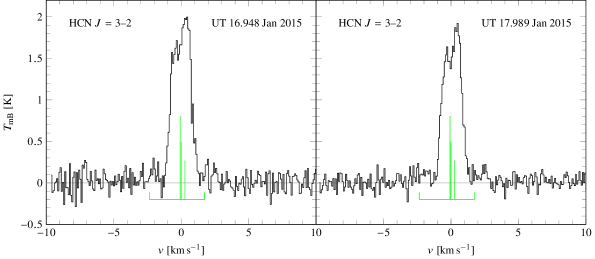
Figure 1: HCN J=3–2 line observed in the spectra of comet C/2014 Q2 (Lovejoy) with the XFFTS2 backend plotted in the cometocentric rest frame. The unresolved HCN hyperfine transitions are shown by the vertical lines.

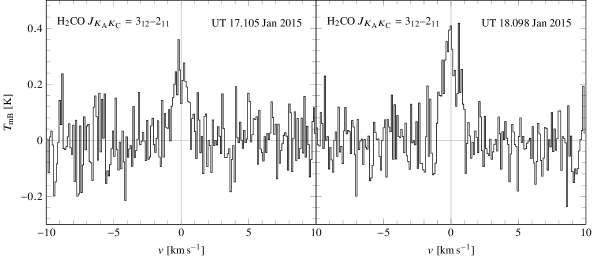
Figure 2: H2CO $\mathrm{J}_{K_{\mathrm{A}}K_{\mathrm{C}}}=3_{12}$–$2_{11}$ line observed in the spectra of comet C/2014 Q2 (Lovejoy) with the XFFTS2 backend plotted in the cometocentric rest frame.

2 Observations

We carried out high resolution observations of comet C/2014 Q2 using the $12\text{\,}\mathrm{m}$ single-dish APEX telescope located at $5100\text{\,}\mathrm{m}$ above sea level in the Atacama desert in northern Chile (Güsten et al., 2006). Our observing program was executed on two nights from UT 16.948 to 18.120 January 2015. The Swedish Heterodyne Facility Instrument (SHeFI; Vassilev et al., 2008) consists of four single-band superconductor–insulator–superconductor (SIS) heterodyne receivers equipped with several backends. We have used the APEX-1 receiver that operates in the $213\text{\,}\mathrm{GHz}275\text{\,}\mathrm{GHz}$ band for our observations in combination with the eXtended bandwidth Fast Fourier Transform Spectrometer (XFFTS) backend. XFFTS offers a high instantaneous bandwidth of $2.5\text{\,}\mathrm{GHz}$ and $32\,768$ channels with a $76.29\text{\,}\mathrm{kHz}$ spectral resolution. The full width at half-maximum (FWHM) of the APEX beam ranges from $23\text{\,}\mathrm{\SIUnitSymbolArcsecond}27\text{\,}\mathrm{\SIUnitSymbolArcsecond}$ at the considered frequencies, which correspond to distances of $10\,000\text{\,}\mathrm{km}12\,000\text{\,}\mathrm{km}$ at the distance of the comet. The line intensities for a given frequency and each of the backend groups in the XFFTS are calibrated with the recommended factors.

Observing conditions were favourable throughout the observing period. The precipitable water vapour over the interval of the observations remained between $3.0\text{\,}\mathrm{mm}3.7\text{\,}\mathrm{mm}$ on the night of 2015 January 16 and between $3.2\text{\,}\mathrm{mm}4.0\text{\,}\mathrm{mm}$ on 2015 January 17. Pointing and focus calibration observations were carried out on Mars and Jupiter because they were close to the comet during the course of our observations. We obtained flux density reference observations of bright standard sources for calibration purposes alternated with the comet observations on a regular basis. The observed sources were the Mira variables o Ceti, IK Tauri and R Doradus, the evolved carbon stars IRC +10216 and R Leporis, and the Orion Molecular Cloud Complex. We used the latest ephemeris provided by JPL’s HORIZONS Solar system service during the observations to track the position and relative motion of the comet with respect to the observer (Giorgini et al., 1996).

Due to the stability of the instrument and the good observing conditions at the APEX site, the calibration of the spectra did not pose special problems. We used the open-source pyspeckit spectroscopic package to read the data files downloaded from the APEX archive (Ginsburg & Mirocha, 2011). pyspeckit supports several file formats including recent versions of the CLASS file format.

Since APEX observations are provided in the Local Standard of Rest Kinematic (LSRK), frequency calibration is required to convert to the cometocentric frame in order to find out the Doppler shift of the observed lines with respect to the rest frequency. Converting velocities from the LSRK frame to the geocentric frame is an operation that depends on the position of the comet and the time of the observation. We adopted the value for the Standard Solar Motion as that used by the APEX staff: $20\text{\,}\mathrm{km}\text{\,}{\mathrm{s}}^{-1}$ towards $\alpha_{1900}=$$$, $\delta_{1900}=$$$ (D. Muders, private communication). Finally the position and velocity of the comet were calculated for each scan with $\approx 30\text{\,}\mathrm{s}$ integration using the callhorizons code to access the JPL HORIZONS ephemerides of comet C/2014 Q2.

Table 1: Observing log of comet C/2014 Q2 (Lovejoy) obtained with APEX.

Date (UT)	$r_{\mathrm{h}}$a	$\Delta$b	$\phi$c	Species	Int.d	Beam FWHM
mm/dd.ddd	(au)	(au)	($\mathrm{\SIUnitSymbolDegree}$)		($\mathrm{min}$)	($\mathrm{\SIUnitSymbolArcsecond}$)
1/16.948	1.3055	0.5281	$42\aas@@fstack{\circ}56$	HCN	$4\aas@@fstack{m}5$	$23\aas@@fstack{\prime\prime}5$
1/17.002	1.3054	0.5287	$42\aas@@fstack{\circ}61$	CH3OH	$22\aas@@fstack{m}5$	$25\aas@@fstack{\prime\prime}8$
1/17.078	1.3052	0.5296	$42\aas@@fstack{\circ}68$	CO	$12\aas@@fstack{m}4$	$27\aas@@fstack{\prime\prime}1$
1/17.105	1.3052	0.5299	$42\aas@@fstack{\circ}71$	H2CO	$3\aas@@fstack{m}5$	$27\aas@@fstack{\prime\prime}6$
1/17.115	1.3051	0.5300	$42\aas@@fstack{\circ}72$	CH3OH	$2\aas@@fstack{m}2$	$25\aas@@fstack{\prime\prime}8$
1/17.989	1.3032	0.5406	$43\aas@@fstack{\circ}46$	HCN	$7\aas@@fstack{m}1$	$23\aas@@fstack{\prime\prime}5$
1/18.030	1.3031	0.5411	$43\aas@@fstack{\circ}50$	CH3OH	$15\aas@@fstack{m}0$	$25\aas@@fstack{\prime\prime}8$
1/18.075	1.3030	0.5417	$43\aas@@fstack{\circ}54$	CO	$10\aas@@fstack{m}6$	$27\aas@@fstack{\prime\prime}1$
1/18.098	1.3030	0.5420	$43\aas@@fstack{\circ}55$	H2CO	$4\aas@@fstack{m}4$	$27\aas@@fstack{\prime\prime}6$
1/18.110	1.3030	0.5421	$43\aas@@fstack{\circ}56$	CH3OH	$2\aas@@fstack{m}6$	$25\aas@@fstack{\prime\prime}8$
1/18.120	1.3029	0.5423	$43\aas@@fstack{\circ}57$	HCN	$3\aas@@fstack{m}1$	$23\aas@@fstack{\prime\prime}5$

• Heliocentric distance.

• Geocentric distance.

• Solar phase angle.

• Total integration time.

We present the observing circumstances and total integration times for each molecule in Table 2. We detected four molecules (HCN, H2CO, CO and CH3OH) and obtained significant upper limits on the emission of the complex molecules acetaldehyde (CH3CHO) and formamide (NH2CHO) by averaging several lines shown in Table 2.

Table 2: Targeted NH2CHO and CH3CHO lines in comet C/2014 Q2 (Lovejoy). The rest-frame line frequencies are obtained from the JPL and CDMS catalogues.

Fig. 1 shows the HCN J = 3–2 transition observed in two different epochs in comet C/2014 Q2 after baseline removal. For this species, we used the line frequencies for the hyperfine structure components from the latest version of the Cologne Database for Molecular Spectroscopy (CDMS; Endres et al., 2016). We show the H2CO $\mathrm{J}_{K_{\mathrm{A}}K_{\mathrm{C}}}=3_{12}$–$2_{11}$ transition in Fig. 2. A marginal detection is obtained for the CO (J = 2–1) line in both the backend group 1 (4.6$\sigma$) and the backend group 2 (5.2$\sigma$) only on the second night of observations (January UT 18.075). In Fig. 3 we show an average of several of the individually resolved methanol lines that are observed simultaneously in one of the receiver settings. We show these CO spectra in Fig. 4. Several methanol transitions were observed simultaneously in the E-CH3OH and A-CH3OH ladders of levels with J = 5, including some that are blended with other transitions. Fig. 5 shows the CH3OH spectrum from January UT 18.042.

The HCN line is detected with high-signal-to-noise ratio (S/N) and is the only detected transition that is expected to be optically thick. However, the observed line asymmetry could be caused by either line-opacity effects in the foreground of the coma or anisotropic outgassing. Since emission lines from other molecules do not have enough S/N to resolve the line profile, we have averaged several of the methanol lines. The averaged line shows a significant redshift and asymmetry (Fig. 3) that seems similarly constructed as in the HCN J = 3–2 transition. The CH3OH emission is predicted to be optically thin. Thus the similarity in the HCN and CH3OH line shapes could be more likely explained by an asymmetric outgassing with preferential emanation from active regions in the nucleus.

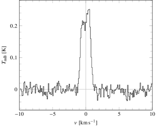
Figure 3: Averaged spectrum of CH3OH emission lines with frequencies $241.700\text{\,}\mathrm{GHz}241.767\text{\,}\mathrm{GHz}241.791\text{\,}\mathrm{GHz}241.879\text{\,}\mathrm{GHz}241.888\text{\,}\mathrm{GHz}$ in comet C/2014 Q2 (Lovejoy) obtained with the XFFTS2 backend.

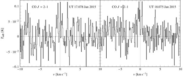
Figure 4: CO-averaged spectrum in comet C/2014 Q2 (Lovejoy) obtained with a $12.3\text{\,}\mathrm{min}$ (left-hand pannel) and $12.6\text{\,}\mathrm{min}$ (right-hand pannel) integration time using the XFFTS2 receiver.

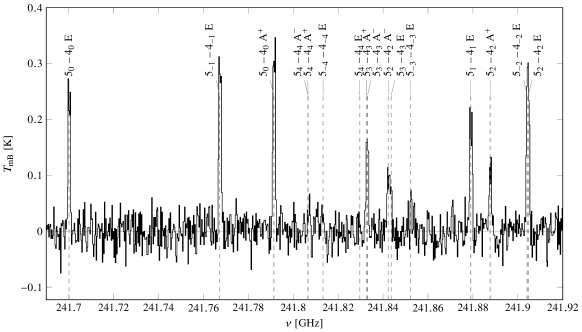
Figure 5: Spectrum of CH3OH emission in comet C/2014 Q2 (Lovejoy) obtained on 2015 January UT 18.042 with a $17.6\text{\,}\mathrm{min}$ total integration time using the XFFTS2 backend. The spectrum was resampled to a $300\text{\,}\mathrm{kHz}$ resolution per channel using a rectangular window function to increase the S/N ratio. CH3OH transitions are indicated by the dashed lines.

Table LABEL:tab:apex shows the line intensity for the transitions detected with 1$\sigma$ uncertainties as the average value of the intensities measured with the XFFTS1 and XFFTS2 backend. Since we did not measure a substantial variation in the production rates of the observed molecules, we have co-added observations of HCN and CH3OH obtained on the same night to increase the S/N of the line emission. Line areas were obtained by numerically integrating the signal over the fitted baseline and the statistical uncertainty in the integrated line intensity was calculated using the root mean square (rms) noise in the background after subtracting the fitted baseline. There is a good agreement between the intensities measured by the XFFTS1 and XFFTS2 backends with a variation $<10\text{\,}\mathrm{\char 37\relax}$ for detections with S/N $>5$. Line frequencies listed in Table LABEL:tab:apex were obtained from the latest online edition of the JPL molecular spectroscopy catalogue (Pickett et al., 1998).

• Variation in line intensity between the two XFFTS backends.

3 Results

3.1 Rotational temperatures

To derive an estimation of the coma kinetic temperature in our radiative transfer model, we calculate the CH3OH rotational temperature obtained in two different dates. Methanol rotational transitions appear in multiple lines at millimetre wavelengths that are well suited to estimate the rotational temperature and excitation conditions in the coma in the optically thin limit. The rotational levels of CH3OH listed in Table LABEL:tab:apex are described with three quantum numbers ($J_{K}\ T_{\mathrm{s}}$) following the notation by Mekhtiev et al. (1999), where J is the total angular momentum, $K$ its projection along the symmetry axis, and $T_{\mathrm{s}}$ is the torsional symmetry state (A⁺, A^-, E₁ or E₂), corresponding to different configurations of the nuclear spin states of the CH3 group. The difference between the E₁ and E₂ states is indicated by the sign of the quantum number $K$ with a positive sign corresponding to E₁ levels and a negative sign to E₂ levels. We have observed several CH3OH transitions around $242\text{\,}\mathrm{GHz}$ that sample rotational levels with quantum number $J=5$.

Assuming that the population distribution of the levels sampled by the emission lines is in local thermodynamical equilibrium (LTE), or described by a Boltzmann distribution characterized by a single temperature, the column density of the upper transition level within the beam, $\langle N_{\mathrm{u}}\rangle$, can be expressed as

$$\langle N_{\mathrm{u}}\rangle=\langle N\rangle\frac{g_{\mathrm{u}}}{Z(T_{\mathrm{rot}})}\exp\left(-\frac{E_{\mathrm{u}}}{k_{\mathrm{B}}T_{\mathrm{rot}}}\right),$$ (1)

where $g_{\mathrm{u}}$ is the degeneracy of the upper level, $Z$ denotes the rotational partition function, which is a function of temperature, $T_{\mathrm{rot}}$ is the rotational temperature, $E_{\mathrm{u}}$ is the energy of the upper state, $k_{\mathrm{B}}$ represents the Boltzmann constant and $\langle N\rangle$ is the total column density averaged over the beam. We use the rotational diagram technique described in detail in Bockelée-Morvan et al. (1994). This methods allows us to determine the rotational temperature, $T_{\mathrm{rot}}$, that describes the relative population of the CH3OH upper states of the observed transitions, by fitting all the transitions detected above the 3$\sigma$ detection limit with both backends.

In Fig. 6 we show the best-fitting of the rotational diagram for the CH3OH lines observed in comet C/2014 Q2 for two different epochs. From the relative intensities of the individual CH3OH lines between levels with quantum numbers J = 5–4 we obtain a rotational temperature of $53\pm 8.\text{\,}\mathrm{K}$ and a beam-averaged column density of $(1.5\pm 0.2)\text{\times}{10}^{11}\text{\,}{\mathrm{cm}}^{-2}$ for January UT 17.012, and $47\pm 6.\text{\,}\mathrm{K}$ and $(1.5\pm 0.3)\text{\times}{10}^{11}\text{\,}{\mathrm{cm}}^{-2}$ for January UT 18.042. We note that blended methanol lines were not included in the analysis. These values of the rotational temperature are comparable with those of other Oort-cloud comets observed at similar heliocentric distances but somewhat lower than other measurements in comet C/2014 Q2 (Biver et al., 2016; Paganini et al., 2017). Since observations obtained with the Keck and IRAM telescopes have a smaller field of view than APEX, they cover the collisional region of the coma which has higher rotational temperature than the outer regions of the coma encompassed in our observations.

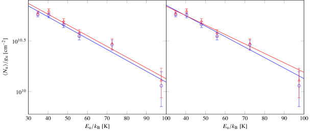
Figure 6: Rotation diagram for CH3OH lines in comet C/2014 Q2 (Lovejoy) including 1$\sigma$ uncertainties from observations obtained on January UT 17.012 (left-hand panel) and January UT 18.042 January (right-hand panel). The natural logarithm of the column density of the upper level divided by its degeneracy is plotted against the energy of the upper level for each transition. The red data points show measurements with the XFFTS1 backend and the blue data points were obtained using XFFTS2, excluding blended lines. The solid lines show the best linear fits to the lines detected with S/N greater than three with an averaged rotational temperature of $53\pm 8.\text{\,}\mathrm{K}$ for January UT 17.012 and $47\pm 6.\text{\,}\mathrm{K}$ for January UT 18.042.

The rotational temperatures derived from CH3OH multiplets are especially useful as they are intermediate between the gas kinetic temperature in the collisional region in the inner coma and the fluorescence equilibrium temperature in the outer parts of the coma (see e.g., Bockelée-Morvan et al., 2004; de Val-Borro et al., 2013; Biver et al., 2016). Using the non-LTE CH3OH model described in Section 3.2, the inferred rotational temperature can be compared to the prediction from the model for a gas kinetic temperature equal to the observed rotational temperature. Assuming a constant gas kinetic temperature of $53\text{\,}\mathrm{K}$, the rotational temperature derived from the CH3OH level population predicted by the model is $45\text{\,}\mathrm{K}$, in agreement with the measured rotational temperature within uncertainties.

3.2 Modelling of line emission

We adopt a radiative transfer method based on the non-LTE Line Modelling Engine code (LIME; Brinch & Hogerheijde, 2010) to derive the production rates that include collisions between neutrals and electrons and radiation trapping effects (see de Val-Borro et al., 2010, and references therein). The radiative pumping of the fundamental vibrational levels, which are induced by solar infrared radiation and subsequently decay to rotational levels in the ground vibrational state, is calculated using the Comet INfrared Excitation (CINE; de Val-Borro et al., 2017b) code. We used a one-dimensional spherically symmetric version of the code with a constant outflow velocity by following the description outlined in Bensch & Bergin (2004), which has been used to model water excitation to interpret cometary observations from the Herschel Space Observatory (see e.g. Bockelée-Morvan et al., 2010, 2012; de Val-Borro et al., 2012; O’Rourke et al., 2013).

We assume an isotropic gas density profile for parent molecules with constant outflow velocity for the gas released from the nucleus (Haser, 1957). Since the observed area covered by the APEX beam has a radius of about $10\,000\text{\,}\mathrm{km}$ at the comet, the assumption of isotropic outgassing is reasonable. The number density of molecules is by

$$n_{\mathrm{p}}(r)=\frac{Q}{4\pi r^{2}v_{\mathrm{exp}}}\,\exp\left(-\frac{r\beta}{v_{\mathrm{exp}}}\right),$$ (2)

where $Q$ is the molecular production rate, $v_{\mathrm{exp}}$ is the expansion velocity and $r$ is the nucleocentric distance. Volatiles that sublimate off the surface of the comet can be photodissociated when they are exposed to solar UV radiation; the photodissociation rate $\beta$ considers the dissociation and ionization of molecules by the radiation from the Sun and determines the spatial distribution of the species. The values of the photodissociation lifetimes for all the molecules are obtained from Crovisier (1994) except for NH2CHO that was extracted from Jackson (1976), and were multiplied by the factor $r_{\mathrm{h}}^{-2}$, where $r_{\mathrm{h}}$ is the heliocentric distance at the time of the observations.

To derive the H2CO production rate we use a coma density model for a daughter species based on the Haser model (Combi et al., 2004) given by

$$n_{\mathrm{d}}(r)=\frac{Q}{4\pi r^{2}v_{\mathrm{exp}}}\,\frac{\beta_{\mathrm{p}}}{\beta_{\mathrm{p}}-\beta_{\mathrm{d}}}\,\left(\exp\left(-\frac{r\beta_{\mathrm{d}}}{v_{\mathrm{exp}}}\right)-\exp\left(-\frac{r\beta_{\mathrm{p}}}{v_{\mathrm{exp}}}\right)\right),$$ (3)

where $\beta_{\mathrm{p}}$ and $\beta_{\mathrm{d}}$ denote the parent and daughter photodissociation rates, respectively. We adopt a parent species photodissociation rate of $\beta_{\mathrm{p}}=$1\text{\times}{10}^{-4}\text{\,}{\mathrm{s}}^{-1}$$. However, the H2CO parent source in cometary coma is currently subject to debate, and the retrieved H2CO production rate is very uncertain.

The derived production rate depends on the model input parameters and collisional excitation rates, as well as on the radiative transfer method that is used to calculate the level populations and synthetic spectrum. We use the molecular data for the observed species available from the Leiden Atomic and Molecular Database (LAMDA; Schöier et al., 2005), including energy levels, statistical weights and collisional rates. Since LAMDA contains collisional data from quantum calculations of each molecule with molecular hydrogen and the main collisional species in cometary coma is H2O, we have scaled the collision rates in the molecular data files by multiplying with the ratio of their molecular masses $m_{\ce{H2O}}/m_{\ce{H2}}$ using the astroquery affiliated package of astropy (Ginsburg et al., 2017). Given the APEX beam size of $~{}10000\text{\,}\mathrm{km}$ at the comet, the contribution of the radiative pumping of vibrational levels by solar radiation is not dominant on the production rates, but there is a noticeable effect on the population levels at distances of the order of the beam FWHM.

To derive molecular abundances of the observed species relative to water, the H2O production rates were obtained from Odin observations and measurements of the OH radical maser lines at $18\text{\,}\mathrm{cm}$ with the Nançay radio telescope (Biver et al., 2015, 2016). During the January 2015 12.8–16.8 observing period, an average water production rate of $(5.0\pm 0.2)\text{\times}{10}^{29}\text{\,}\mathrm{mol}\text{\,}{\mathrm{s}}^{-1}$ was measured. Based on Nançay and Odin observations, we adopt a value for $Q_{\ce{H2O}}$ of $6\text{\times}{10}^{29}\text{\,}\mathrm{mol}\text{\,}{\mathrm{s}}^{-1}$ for the period of the APEX observations. We assumed that the $A$ and $E$ forms of CH3OH are equally abundant in our calculation. As an estimate of the kinetic gas temperature in the coma we use the value of the rotational temperature derived in Section 3.1 from multiple CH3OH transitions observed simultaneously, $53\text{\,}\mathrm{K}$. We assume that the kinetic gas temperature and outgassing velocity are constant throughout the coma in our model. The outgassing velocity in the coma is obtained from the half width at half-maximum (HWHM) of a Gaussian fit to the CH3OH transitions detected with high S/N. The HWHM was further reduced by $15\text{\,}\mathrm{\char 37\relax}$ to take into account the increase in line width due to thermal Doppler broadening, resulting in a value of $0.8\text{\,}\mathrm{km}\text{\,}{\mathrm{s}}^{-1}$. This expansion velocity agrees with the value determined using the IRAM $30\text{\,}\mathrm{m}$ telescope (Biver et al., 2016).

Once the level populations are calculated for each grid point in the cometary model, the synthetic emission line profiles are obtained by ray tracing along straight lines of sight using LIME. Image cubes are produced for each transition in standard FITS format. The resulting line spectrum was obtained by convolution with the APEX beam at each frequency given in Table 2. The line intensity in the synthetic spectrum is then compared with the observed integrated intensities, and the model is varied accordingly using a different value of the production rate until there is good agreement.

Sensitive upper limits on acetaldehyde and formamide are calculated by averaging the strongest lines in the wavelength range covered by our observations, as predicted by our model. Table 2 shows the chosen emission lines covered by our observations in any of the receiver settings with either of the XFFTS backends. All the considered CH3CHO transitions are of the E form. We assume that the ratio of A and E forms is also the statistical equilibrium value to derive the production rate upper limit for CH3CHO. The upper limits to the averaged line intensities were obtained by integrating the flux over a width of $1.6\text{\,}\mathrm{km}\text{\,}{\mathrm{s}}^{-1}$ derived from the high-S/N methanol lines. Using a spherically symmetric Haser model, the resulting 3$\sigma$ upper limits are $6\text{\times}{10}^{26}\text{\,}\mathrm{mol}\text{\,}{\mathrm{s}}^{-1}{10}^{26}\text{\,}\mathrm{mol}\text{\,}{\mathrm{s}}^{-1}$ for CH3CHO and NH2CHO, respectively.

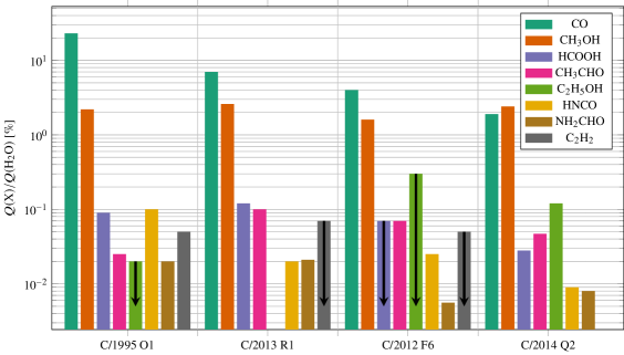
Figure 7: Observed mixing ratios relative to water in comets C/1995 O1 (Hale-Bopp), C/2013 R1 (Lovejoy), C/2012 F6 (Lemmon) and C/2014 Q2 (Lovejoy) from this work and from Dello Russo et al. (2001), Paganini et al. (2014a), Paganini et al. (2014b), Biver et al. (2014) and Biver et al. (2015). Upper limits are indicated by the black vertical arrows.

Table 4 summarizes the production rates and mixing ratios of the detected volatiles in C/2014 Q2 with respect to H2O and a comparison to other measurements using the IRAM $30\text{\,}\mathrm{m}$ telescope. Statistical uncertainties are 1$\sigma$ rms noise from the integrated intensities. We confirm that C/2014 Q2 is rather depleted in CO and has low HCN and H2CO abundances. The measured production rates are consistent with values derived for this object from other facilities at radio wavelengths (Biver et al., 2016; Wirström et al., 2016).

Table 4: Production rates in C/2014 Q2 (Lovejoy) with statistical uncertainties measured by APEX between 2015 January 16–18.

Molecule	$Q$	$Q/Q_{\ce{H2O}}$a	$Q/Q_{\ce{H2O}}$b	Range $Q/Q_{\ce{H2O}}$c
	($\mathrm{mol}\text{\,}{\mathrm{s}}^{-1}$)	($\mathrm{\char 37\relax}$)	($\mathrm{\char 37\relax}$)	Lower ($\mathrm{\char 37\relax}$)	Upper ($\mathrm{\char 37\relax}$)
HCN	$(6.1\pm 0.1)\text{\times}{10}^{26}$	$0.1$	$0.09$	$0.08$	$0.25$
CO	$(1.2\pm 0.3)\text{\times}{10}^{28}$	$2.0$	$1.8$	$2$	$33$
H2CO	$(1.3\pm 0.2)\text{\times}{10}^{27}$	$0.2$	$0.3$	$0.1$	$1.4$
CH3OH	$(1.3\pm 0.1)\text{\times}{10}^{28}$	$2.2$	$2.4$	$0.6$	$6$
CH3CHO	$<6\text{\times}{10}^{26}$	$<0.1$	$0.047$	$0.052$	$0.08$
NH2CHO	$<1\text{\times}{10}^{26}$	$<0.02$	$0.008$	$0.012$	$0.021$

• Abundances measured by APEX relative to water. An average H2O production rate of $(6.0\pm 0.6)\text{\times}{10}^{29}\text{\,}\mathrm{mol}\text{\,}{\mathrm{s}}^{-1}$ was obtained by interpolation of Odin observations during the period January 30 to February 3 and Nançay measurements on January 12–16 (Biver et al., 2015). CH3CHO and NH2CHO abundances are derived 3$\sigma$ upper limits.

• Relative abundances obtained by the $30\text{\,}\mathrm{m}$ IRAM telescope (Biver et al., 2015).

• Range of typical abundances measured in a sample of comets.

4 Discussion

Our upper limits on CH3CHO and NH2CHO are consistent with the mixing ratios measured in C/2014 Q2 by Biver et al. (2015). These molecules are amongst a suite of organic molecules found in comets: CH3OH (methanol), CH3CHO (acetaldehyde), C2H5OH (ethanol), HCOOH (formic acid), HNCO (isocyanic acid) and NH2CHO (formamide) that may share a common formation pathway from CO (e.g., Mumma & Charnley, 2011; Cochran et al., 2015). In this scenario CO molecules are frozen out on cold dust grains and hydrogen atom additions in CO ice produce the formyl radical from which larger molecules are built up by subsequent heavy atom additions and further H additions in the reaction sequences (e.g., Charnley & Rodgers, 2008; Herbst & van Dishoeck, 2009):

(4)

(5)

Most of these reactions have been demonstrated in the laboratory (e.g., Linnartz et al., 2015).

A wide range of CO mixing ratios has been measured in comets, with C/2014 Q2 having one of the lowest. By comparing the mixing ratios of complex organic molecules with their CO content, we can explore the feasibility of these molecules having had their precometary origin on cold interstellar/nebular dust grains (e.g., Disanti & Mumma, 2008). Fig. 7 summarizes the relative mixing ratios of eight organic molecules as measured in four comets which displayed a range of CO mixing ratios. Mixing ratios in comets C/1995 O1 (Hale-Bopp), C/2013 R1 (Lovejoy), C/2012 F6 (Lemmon) and C/2014 Q2 (Lovejoy) are from this work and from the compilations of Biver et al. (2014, 2015), except for C2H2 where values are taken from Dello Russo et al. (2001), Paganini et al. (2014a), and Paganini et al. (2014b). Fig. 7 shows that the CH3OH mixing ratio is constant and independent of the amount of CO present. Although C/2014 Q2 has the least CO its methanol ratio is one of the largest in the sample, with about $56\text{\,}\mathrm{\char 37\relax}$ of the original CO having been converted. This suggests that CH3OH formation is highly efficient, and is probably only limited by the availability of H atoms on the surface. High CO conversion efficiencies have been reported in laboratory studies. The mixing ratios of both HNCO and NH2CHO both increase with that of CO, although the decline of NH2CHO is less pronounced. For CH3CHO and C2H5OH the trend is puzzling and seems to be inconsistent with their formation in sequence LABEL:reaction:4. C/2013 R1 has the highest mixing ratios of CH3CHO but C/2014 Q2, with the lowest CO content ($Q(\ce{CO})/Q(\ce{H2O})=$1.9\text{\,}\mathrm{\char 37\relax}$$), is more enriched in CH3CHO than C/1995 O1 ($Q(\ce{CO})/Q(\ce{H2O})=$23\text{\,}\mathrm{\char 37\relax}$$). This suggests that CH3CHO and C2H5OH have alternative ice formation processes that are unconnected to CO. Hydrogenation and O atom addition sequences starting from C2H2 are possible (e.g., Charnley, 2004) but is unsupported by the trend of their mixing ratios with the existing C2H2 data. C/2014 Q2 does have the lowest HCOOH mixing ratio but a decline with CO ratio only appears at $Q(\ce{CO})/Q(\ce{H2O})\approx$7\text{\,}\mathrm{\char 37\relax}$$.

We conclude that there is some observational support for atom addition reactions on cold dust being the origin of some of these molecules. It is not clear why the extreme CO ratio of C/1995 O1 only leads to modest abundances of complex molecules (apart from HNCO) and why C/2013 R1 has the largest abundances. An important caveat to the above analysis is that we have not considered possible, and essentially unknowable, variations in the abundances of the heavy atoms (C, O, N) in the gas where the precometary ices formed. A larger statistical sample of similar cometary observations will be required to further test these ideas.

5 Conclusions

The chemical composition of the long-period very active comet C/2014 Q2 (Lovejoy) has been investigated using submillimetre spectroscopic molecular observations obtained with the $12\text{\,}\mathrm{m}$ APEX telescope. We have presented the results of our data analysis of the observations of HCN, H2CO, CO and CH3OH and derivation of their molecular abundances using a non-LTE molecular excitation method. Based on the average of the strongest lines in the wavelength range covered by our observations, we have also derived upper limits on the complex molecules acetaldehyde (CH3CHO) and formamide (NH2CHO).

We have presented a three-dimensional coma model that allows a detailed interpretation of cometary observations and computation of the production rates from the observed line transition intensities. We calculate the molecular excitation in the coma using the LIME code by Brinch & Hogerheijde (2010). This model includes collisional excitation of the rotational levels by water, spontaneous and induced emission, and radiation trapping effects. The radiative pumping of the fundamental vibrational levels induced by solar infrared radiation which subsequently decay to rotational levels in the ground vibrational state is calculated using the CINE code (de Val-Borro et al., 2017a). Although we have used an isotropic outgassing geometry to interpret our observations, the capability of the code to handle multidimensional geometries, e.g., collimated jets or distributed sources in the coma, will be useful for the interpretation of future comet observations carried out with ALMA.

Based on a spherically symmetric Haser model with constant outflow velocity, and assuming a constant kinetic gas temperature from observations of multiple CH3OH transitions in comet C/2014 Q2, we derive molecular production rates for HCN, H2CO, CO and CH3OH, and upper limits for CH3CHO and NH2CHO. The methanol rotational temperature of $53\pm 8.\text{\,}\mathrm{K}$ derived from multiple lines using the rotational diagram technique is lower and consistent within the accuracy of the detections with the value of $67\pm 15.\text{\,}\mathrm{K}$ for CH3OH determined by Biver et al. (2016). Our measurement is also lower than the H2O rotational temperature of $78\pm 1.\text{\,}\mathrm{K}$ retrieved by Paganini et al. (2017). This inconsistency in the derived rotational temperatures between infrared and radio measurements can be reconciled taking into account that observations with small beam size (infrared) sample a hotter region of the coma while observations with a larger beam (radio) include cooler material and thus exhibit a lower rotational temperature. We discussed the possible connection between the low CO mixing ratios and the relative abundances of complex molecules in C/2014 Q2 in comparison with other comets. Further observations of future cometary apparitions, similar to those presented here, will provide important information on chemical formation pathways and physical conditions in the protosolar molecular cloud core and/or the protosolar nebula (e.g., Mandt et al., 2015; Willacy et al., 2015).

Acknowledgements

This work was supported by NASA’s Planetary Astronomy Program. This publication is based on data acquired with the Atacama Pathfinder Experiment (APEX) telescope. APEX is a collaboration between the Max-Planck-Institut für Radioastronomie, the European Southern Observatory, and the Onsala Space Observatory. The APEX observations were conducted under the observing proposal O-094.F-9307(A). The authors would like to thank the referee, J. Crovisier, for giving valuable comments. We gratefully acknowledge the support of the APEX staff, in particular to Michael Olberg and Dirk Muders, for their assistance with data analysis.

References

- A’Hearn et al. (1995) A’Hearn M. F., Millis R. L., Schleicher D. G., Osip D. J., Birch P. V., 1995, Icarus, 118, 223
- Bensch & Bergin (2004) Bensch F., Bergin E. A., 2004, ApJ, 615, 531
- Biver et al. (2014) Biver N., et al., 2014, A&A, 566, L5
- Biver et al. (2015) Biver N., et al., 2015, Science Advances, 1, 1500863
- Biver et al. (2016) Biver N., et al., 2016, A&A, 589, A78
- Bockelée-Morvan et al. (1994) Bockelée-Morvan D., Crovisier J., Colom P., Despois D., 1994, A&A, 287, 647
- Bockelée-Morvan et al. (2004) Bockelée-Morvan D., Crovisier J., Mumma M. J., Weaver H. A., 2004, in Festou M. C., Keller H. U., Weaver H. A., eds, in Comets II. Univ. Arizona Press, pp 391–423
- Bockelée-Morvan et al. (2010) Bockelée-Morvan D., et al., 2010, A&A, 518, L149
- Bockelée-Morvan et al. (2012) Bockelée-Morvan D., et al., 2012, A&A, 544, L15
- Brinch & Hogerheijde (2010) Brinch C., Hogerheijde M. R., 2010, A&A, 523, A25
- Charnley (2004) Charnley S. B., 2004, Advances in Space Research, 33, 23
- Charnley & Rodgers (2008) Charnley S. B., Rodgers S. D., 2008, Space Sci. Rev., 138, 59
- Cochran et al. (2015) Cochran A. L., et al., 2015, Space Sci. Rev., 197, 9
- Combi et al. (2004) Combi M. R., Harris W. M., Smyth W. H., 2004, in Festou, M. C., Keller, H. U., & Weaver, H. A. ed., Comets II. Univ. Arizona Press, pp 523–552
- Cordiner et al. (2017) Cordiner M. A., et al., 2017, ApJ, 838, 147
- Crovisier (1994) Crovisier J., 1994, J. Geophys. Res., 99, 3777
- Dello Russo et al. (2001) Dello Russo N., Mumma M. J., DiSanti M. A., Magee-Sauer K., Novak R., 2001, Icarus, 153, 162
- Dello Russo et al. (2016) Dello Russo N., Kawakita H., Vervack R. J., Weaver H. A., 2016, Icarus, 278, 301
- Disanti & Mumma (2008) Disanti M. A., Mumma M. J., 2008, Space Sci. Rev., 138, 127
- Endres et al. (2016) Endres C. P., Schlemmer S., Schilke P., Stutzki J., Müller H. S. P., 2016, Journal of Molecular Spectroscopy, 327, 95
- Ginsburg & Mirocha (2011) Ginsburg A., Mirocha J., 2011, PySpecKit: Python Spectroscopic Toolkit (ascl:1109.001)
- Ginsburg et al. (2017) Ginsburg A., et al., 2017, astropy/astroquery: v0.3.6 with fixed license, doi:10.5281/zenodo.826911, https://doi.org/10.5281/zenodo.826911
- Giorgini et al. (1996) Giorgini J. D., et al., 1996, in AAS/Division for Planetary Sciences Meeting Abstracts #28. p. 1158
- Güsten et al. (2006) Güsten R., Nyman L. Å., Schilke P., Menten K., Cesarsky C., Booth R., 2006, A&A, 454, L13
- Haser (1957) Haser L., 1957, Bull. Soc. Roy. Sci. Liège, 43, 740
- Herbst & van Dishoeck (2009) Herbst E., van Dishoeck E. F., 2009, ARA&A, 47, 427
- Hogerheijde & van der Tak (2000) Hogerheijde M. R., van der Tak F. F. S., 2000, A&A, 362, 697
- Jackson (1976) Jackson W. M., 1976, NASA Special Publication, 393
- Linnartz et al. (2015) Linnartz H., Ioppolo S., Fedoseev G., 2015, International Reviews in Physical Chemistry, 34, 205
- Lovejoy et al. (2014) Lovejoy T., Jacques C., Pimentel E., Barros J., 2014, Central Bureau Electronic Telegrams, 3934
- Mandt et al. (2015) Mandt K. E., Mousis O., Bockelée-Morvan D., Russell C. T., 2015, Space Sci. Rev., 197, 5
- Mekhtiev et al. (1999) Mekhtiev M. A., Godfrey P. D., Hougen J. T., 1999, Journal of Molecular Spectroscopy, 194, 171
- Mumma & Charnley (2011) Mumma M. J., Charnley S. B., 2011, ARA&A, 49, 471
- O’Rourke et al. (2013) O’Rourke L., et al., 2013, ApJ, 774, L13
- Paganini et al. (2014a) Paganini L., et al., 2014a, AJ, 147, 15
- Paganini et al. (2014b) Paganini L., et al., 2014b, ApJ, 791, 122
- Paganini et al. (2017) Paganini L., Mumma M. J., Gibb E. L., Villanueva G. L., 2017, ApJ, 836, L25
- Pickett et al. (1998) Pickett H. M., Poynter R. L., Cohen E. A., Delitsky M. L., Pearson J. C., Müller H. S. P., 1998, J. Quant. Spectrosc. Radiative Transfer, 60, 883
- Schöier et al. (2005) Schöier F. L., van der Tak F. F. S., van Dishoeck E. F., Black J. H., 2005, A&A, 432, 369
- Vassilev et al. (2008) Vassilev V., et al., 2008, A&A, 490, 1157
- Willacy et al. (2015) Willacy K., et al., 2015, Space Sci. Rev., 197, 151
- Wirström et al. (2016) Wirström E. S., Lerner M. S., Källström P., Levinsson A., Olivefors A., Tegehall E., 2016, A&A, 588, A72
- de Val-Borro & Wilson (2016) de Val-Borro M., Wilson T. G., 2016, CRETE: Comet RadiativE Transfer and Excitation, Astrophysics Source Code Library (ascl:1612.009)
- de Val-Borro et al. (2010) de Val-Borro M., et al., 2010, A&A, 521, L50
- de Val-Borro et al. (2012) de Val-Borro M., et al., 2012, A&A, 546, L4
- de Val-Borro et al. (2013) de Val-Borro M., et al., 2013, A&A, 559, A48
- de Val-Borro et al. (2017a) de Val-Borro M., Cordiner M. A., Milam S. N., Charnley S. B., 2017a, CINE: Comet INfrared Excitation, Astrophysics Source Code Library (ascl:1708.002)
- de Val-Borro et al. (2017b) de Val-Borro M., Cordiner M. A., Milam S. N., Charnley S. B., 2017b, JOSS, 2017