Bell’s theorem in automata theory

Abstract

Bell’s theorem is reformulated and proved in the pure mathematical terms of automata theory, avoiding any physical or ontological notions. It is stated that no pair of finite probabilistic sequential machines can reproduce in its output the statistical results of the quantum-physical Bell test experiment if each machine is independent of the respective remote input.

Keywords: Bell’s theorem, Bell test experiment, Bell-CHSH inequality, probabilistic sequential machines, quantum sequential machines.

1 Introduction

Bell’s theorem (Bell, 1964) was praised as one of the most profound discoveries of science (Stapp, 1975). Even more than 50 years after its discovery there is a vivid discussion of its meaning and its impact in a plenty of scientific papers. And the thought experiment on which the theorem is based, the Bell test experiment, is performed each year in new variants (e.g., https://thebigbelltest.org).

Bell’s theorem states that “no physical theory which is realistic and also local in a specified sense can agree with all of the statistical implications of Quantum Mechanics” (Shimony, 2016). However, the meaning of this proposition is not easy to understand, neither its consequences for cryptographic protocols (e.g., Ekert, 1991).

In the following the theorem will be reformulated for automata theory in a pure mathematical way without any physical or ontological notions. For that purpose the arrangement of an ideal Bell test experiment is represented by a pair of automata, deterministic or probabilistic sequential machines, which produce an output after each input given by local operators or independent random generators. The theorem states that no such pair can reproduce the statistical results of the quantum-physical Bell test experiment in its output data if each machine is independent on the input of the respective remote machine, or loosely speaking: without data transmission between the remote sides.

After presenting a short sketch of the physical Bell test experiment, we will give a brief introduction to the theory of sequential machines and then prove the theorem.

2 Bell test experiment

The fundamental idea of the Bell test experiment has a long lasting history: Einstein, Podolsky, and Rosen (EPR 1935) developed a quantum-physical thought experiment that displayed strange non-local correlations between the results of remote measurements on a pair of particles, depending on the choice of the measured quantity. The setting of this thought experiment was simplified by Bohm (1951) and inspired Bell (1964) to his theorem. Experimentalists like Clauser, Horne, Shimony, and Holt (CHSH 1969) transformed Bell’s thought experiment into a real one, using photon pairs, with the first sufficient realization by Aspect et al. (1982).

For our purpose a coarse sketch of an ideal Bell test experiment without any physical details is sufficient.

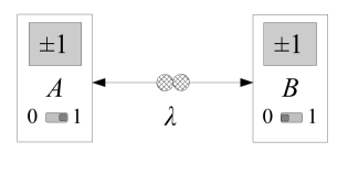
Figure 2.1: Bell test experiment

A single run of the experiment starts by sending a pair of particles $\lambda$ from a source, each particle in another direction, to the measurement devices $A$ and $B$ (fig. 2.1). Each measurement device has an input switch with two positions $0$, $1$, where local operators or independent random generators can select one of two different measurements to be performed. So on each side one of two possible quantities $A_{0}$, $A_{1}$, respectively $B_{0}$, $B_{1}$, is measured. The display of the apparatus shows the measurement result, which is in all cases $-1$ or $1$.

This arrangement enables the measurement of one of four possible pairs $(A_{0},B_{0})$, $(A_{0},B_{1})$, $(A_{1},B_{0})$, $(A_{1},B_{1})$ in each run of the experiment, from which the corresponding product $A_{0}B_{0}$, $A_{0}B_{1}$, $A_{1}B_{0}$, or $A_{1}B_{1}$ is computed, which has the value $-1$ or $1$. The procedure will be repeated with different random measurement selections. After several runs the mean values of the products $\overline{A_{0}B_{0}}$, $\overline{A_{0}B_{1}}$, $\overline{A_{1}B_{0}}$, $\overline{A_{1}B_{1}}$ are used to compute the following expression

$$\overline{A_{0}B_{0}}+\overline{A_{0}B_{1}}+\overline{A_{1}B_{0}}-\overline{A_{1}B_{1}}\textrm{,}$$

which in the long run should approximate the theoretical given expectation value

$$\bigl{\langle}E_{\mathrm{CHSH}}\bigr{\rangle}=\bigl{\langle}A_{0}B_{0}\bigr{\rangle}+\bigl{\langle}A_{0}B_{1}\bigr{\rangle}+\bigl{\langle}A_{1}B_{0}\bigr{\rangle}-\bigl{\langle}A_{1}B_{1}\bigr{\rangle}=\bigl{\langle}A_{0}B_{0}+A_{0}B_{1}+A_{1}B_{0}-A_{1}B_{1}\bigr{\rangle}\textrm{.}$$

In probability theory for any four random variables $A_{0}$, $A_{1}$, $B_{0}$, $B_{1}$ with the image $\{-1,1\}$ on an event space $(\Omega,\mathcal{A})$ the absolute value of this expectation value is bounded according the Bell-CHSH inequality (Clauser et al., 1969) by the value $2$ (cf. app. A), so for any probability measure $\mu$ on $(\Omega,\mathcal{A})$

$$\bigl{|}\bigl{\langle}E_{\mathrm{CHSH}}\bigr{\rangle}\bigr{|}\leq 2\textrm{.}$$

However, quantum theory predicts in some cases values above 2 (and below or equal $2\sqrt{2}$). That was confirmed by the measurement results of various quantum-physical Bell test experiments (e.g., Aspect et al. 1982). So the violation of the Bell-CHSH inequality is an experimental fact of quantum physics.

3 Probabilistic sequential machines

A sequential machine (SM) is an abstract automaton that after each input produces an output and may change its internal state. $I$, $O$, $S$ denote the sets of input symbols, output symbols (also called input and output alphabet) and states. A SM is called finite if all these sets $I$, $O$, $S$ are finite.

A deterministic SM (DSM) is defined by a quintuple $(I,O,S,s_{0},f)$ where $s_{0}\in S$ is the initial state and the deterministic machine function

$$f\colon I\times S\rightarrow O\times S,(i,s)\mapsto(o,t)=f(i,s)$$

determines the output $o$ and the new state $t$ after an input $i$ in state $s$. For a probabilistic SM the new state $t$ and the output symbol $o$ are randomly chosen after each input.

A finite probabilistic SM (FPSM) is defined by a quintuple $(I,O,S,p_{0},p)$ with finite $I$, $O$, $S$, an initial state distribution function

$$p_{0}\colon S\rightarrow[0,1],s\mapsto p_{0}(s)$$

with

$$\sum_{s\in S}p_{0}(s)=1,$$

and a probabilistic machine function

$$p\colon O\times S\times I\times S\rightarrow[0,1],(o,t,i,s)\mapsto p(o,t\mid i,s)\textrm{,}$$

which gives the probability to get the output $o$ and the new state $t$ after the input $i$ in state $s$, with

$$\sum_{o\in O}\sum_{t\in S}p(o,t\mid i,s)=1$$

for all $i\in I,s\in S$.

A FPSM $(I,O,S,p_{0},p)$ is deterministic if the image of the functions $p_{0}$ and $p$ is $\{0,1\}.$ In that case an equivalent finite DSM $(I,O,S,s_{0},f)$ is defined by the initial state $s_{0}\in S$ which is uniquely determined by $p_{0}(s_{0})=1$, and the function $f$ which is given by the set of pairs $((i,s)\mapsto(o,t))$ with $p(o,t\mid i,s)=1$.

4 Simulation of Bell test experiments with FPSMs

The theory of FPSMs is versatile enough to describe any simulation of the Bell test experiment with a computer or an electronic circuit. We start with a single FPSM for the simulation where the output is a pair $o=(A,B)\in O=\{-1,1\}^{2}$ that represents the measurement results. The input is given as a triple $i=(a,b,\lambda)\in I=\{0,1\}^{2}\times\varLambda$, where $a$ and $b$ represent the experimenters choices and $\lambda\in\varLambda$ some not further specified properties of the particle pair, which can be used like the internal states $S$ for a computational model of the experiment. The simulation FPSM is denoted by

$$M=(\{0,1\}^{2}\times\varLambda,\{-1,1\}^{2},S,p_{0},p)\textrm{.}$$

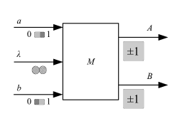
Figure 4.1: Simulation of the Bell test experiment with a FPSM

It is obvious that the FPSM simulation has less constraints then the original experiment: the outputs may not represent four measurable quantities $A_{0},A_{1},B_{0},B_{1}$. So we have to use a slightly more general notation.

4.1 Simulation protocol

In each run of the simulation the FPSM is prepared randomly to an initial state $s\in S$ according to the probability distribution $p_{0}$, and an input symbol $\lambda\in\varLambda$ is entered, randomly selected according to a probability distribution $p_{\varLambda}$. Furthermore the input symbols $a,b\in\{0,1\}$ are entered by the operators or automatically by independent random generators. Then the output symbols $A,B\in\{-1,1\}$ (and the new state $t\in S$) are given by the machine according to the probabilistic machine function $p$.

The product of the output symbols $A\cdot B$ is recorded by the operator together with the corresponding pair of input symbols $(a,b)$

$$\left.AB\right.\mid_{a,b}$$

After a series of runs (or multiple series for the different combinations of the values of $a$, $b$) the mean values of the recorded products for the different input symbols are computed

$$\overline{\left.AB\right.}\mid_{0,0}\textrm{, }\overline{\left.AB\right.}\mid_{0,1}\textrm{, }\overline{\left.AB\right.}\mid_{1,0}\textrm{, }\overline{\left.AB\right.}\mid_{1,1}\textrm{,}$$

as well as the Bell-CHSH expression

$$\overline{E}_{\mathrm{CHSH}}=\overline{\left.AB\right.}\mid_{0,0}+\overline{\left.AB\right.}\mid_{0,1}+\overline{\left.AB\right.}\mid_{1,0}-\overline{\left.AB\right.}\mid_{1,1}\textrm{.}$$

In the special case of a Bell test simulation this value should approximate in the long run the theoretical given expectation value of the Bell-CHSH expression

$$\bigl{\langle}E_{\textrm{CHSH}}\bigr{\rangle}=\bigl{\langle}A_{0}B_{0}\bigr{\rangle}+\bigl{\langle}A_{0}B_{1}\bigr{\rangle}+\bigl{\langle}A_{1}B_{0}\bigr{\rangle}-\bigl{\langle}A_{1}B_{1}\bigr{\rangle}\textrm{.}$$

But in general the corresponding theoretical expression for the PSM is a sum of conditional expectation values

$$\tilde{E}_{\mathrm{CHSH}}=\bigl{\langle}AB\bigr{\rangle}\mid_{0,0}+\bigl{\langle}AB\bigr{\rangle}\mid_{0,1}+\bigl{\langle}AB\bigr{\rangle}\mid_{1,0}-\bigl{\langle}AB\bigr{\rangle}\mid_{1,1}\textrm{,}$$

which can be computed by

$$\bigl{\langle}AB\bigr{\rangle}\mid_{a,b}=\sum_{A\in\{-1,1\}}\sum_{B\in\{-1,1\}}AB\cdot q(A,B|a,b)$$

with the conditional output probability to get the output $(A,B)$ after input $(a,b)$

$$q\left(A,B\mid a,b\right)=\sum_{\lambda\in\varLambda}\sum_{s\in S}\sum_{t\in S}p(A,B,t\mid a,b,\lambda,s)p_{\Lambda}(\lambda)p_{0}(s)\textrm{.}$$

Example 1.

The following table gives the probabilistic machine functions of several simple FPSMs for the simulation of the Bell test experiment.

	$q(A,B\mid a,b)=p(A,B,t\mid a,b,\lambda,s)$	$\bigl{\langle}AB\bigr{\rangle}|{}_{0,0}$	$\bigl{\langle}AB\bigr{\rangle}|_{0,1}$	$\bigl{\langle}AB\bigr{\rangle}|_{1,0}$	$\bigl{\langle}AB\bigr{\rangle}|_{1,1}$	$\tilde{E}_{\mathrm{CHSH}}$
$M_{1}$	$\frac{1}{4}$	$0$	$0$	$0$	$0$	$0$
$M_{2}$	$\delta_{A,1}\delta_{B,1}$	$1$	1	$1$	$1$	$2$
$M_{3}$	$\delta_{A,1}\delta_{B,1-2ab}$	$1$	1	$1$	$-1$	$4$
$M_{4}$	$\frac{1}{2}\delta_{A,1}\delta_{B,1-2ab}+\frac{1}{2}\delta_{A,-1}\delta_{B,2ab-1}$	$1$	1	$1$	$-1$	$4$
$M_{5}$	$\frac{2-\sqrt{2}}{8}+\frac{\sqrt{2}}{8}(2\delta_{A,B}+2ab-4ab\delta_{A,B})$	$\frac{\sqrt{2}}{2}$	$\frac{\sqrt{2}}{2}$	$\frac{\sqrt{2}}{2}$	$-\frac{\sqrt{2}}{2}$	$2\sqrt{2}$

Table 1: Probabilistic machine functions and expectations of the example FPSMs

There is no dependence on internal states or $\lambda$-input, so we assume $S=\{s_{0}\}$ with $p_{0}(s_{0})=1$ and $\varLambda=\{\lambda_{0}\}$ with $p_{\Lambda}(\lambda_{0})=1$. In this case the probabilistic machine function is equal to the conditional output probability $q(A,B\mid a,b)=p(A,B,t\mid a,b,\lambda,s)$ for all $\lambda\in\varLambda$; $s,t\in S$. $\delta_{x,y}$ is the Kronecker symbol and has the value $1$ if $x=y$ and $0$ otherwise.

The output of FPSM $M_{1}$ is evenly distributed and uncorrelated random, whereas $M_{2}$ gives the constant output $(1,1)$. FPSM $M_{3}$ modifies the constant output $1$ in the case that $a$ and $b$ have the value $1.$ FPSM $M_{4}$ is a mixture of $M_{3}$ and its negative counterpart and simulates a Popescu-Rohrlich box (PR box). FPSM $M_{5}$ is the simulation of a quantum-physical Bell test.

The FPSMs $M_{2}$ and $M_{3}$ are deterministic. The value of $\tilde{E}_{\textrm{CHSH}}$ indicates that the FPSMs $M_{3}$, $M_{4}$, $M_{5}$ violate the Bell-CHSH inequality.

The free web app https://bell.qlwi.de can be used to perform Bell test simulations with these FPSMs on any PC, tablet, or smartphone with an up-to-date internet browser.

4.2 Machine composition and stochastic independence of the machine functions

The example FPSM $M_{5}$ demonstrates that it is possible to simulate a Bell experiment with a FPSM and get the same statistical results as with a quantum-physical experiment.

However, to shed some light on Bell’s theorem the simulation has to be performed with a pair of two separated FPSMs, as sketched by the circuit diagram in fig. 4.2).

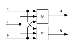
Figure 4.2: Simulation of the Bell test experiment with two FPSMs

Both FPSMs

$$M^{\mathfrak{a}}=(\{0,1\}^{2}\times\varLambda,\{-1,1\},S^{\mathfrak{a}},p_{0}^{\mathfrak{a}},p^{\mathfrak{a}})$$

$$M^{\mathfrak{b}}=(\{0,1\}^{2}\times\varLambda,\{-1,1\},S^{\mathfrak{b}},p_{0}^{\mathfrak{b}},p^{\mathfrak{b}})$$

receive the same input (this also ensures synchronization). But each one gives only one output $A\in\{-1,1\}$, respectively $B\in\{-1,1\}.$ The pair $(M^{\mathfrak{a}},M^{\mathfrak{b}})$ can be considered as a compound FPSM

$$M^{\mathfrak{ab}}=(\{0,1\}^{2}\times\varLambda,\{-1,1\}^{2},S^{\mathfrak{a}}\times S^{\mathfrak{b}},p_{0}^{\mathfrak{a}}p_{0}^{\mathfrak{b}},p^{\mathfrak{a}}p^{\mathfrak{b}})\textrm{,}$$

where the probabilistic machine function and the initial state distribution function are given as products of the corresponding functions of the components, which reflects the independence of the machines. For that reason not every FPSM can be replaced by a pair.

Example 2.

The FPSMs $M_{4}$ and $M_{5}$ of example 1 cannot be replaced by pair, but the FPSMs $M_{1}$, $M_{2}$, and $M_{3}$ can. If we assume $S^{\mathfrak{a}}=\{s_{0}^{\mathfrak{a}}\}$, $S^{\mathfrak{b}}=\{s_{0}^{\mathfrak{b}}\}$ and $s_{0}=(s_{0}^{\mathfrak{a}},s_{0}^{\mathfrak{b}})$ with $p_{0}^{\mathfrak{a}}(s_{0}^{\mathfrak{a}})=p_{0}^{\mathfrak{b}}(s_{0}^{\mathfrak{b}})=1$, then $M_{1}=(\{0,1\}^{2}\times\{\lambda_{0}\},\{-1,1\}^{2},\{s_{0}\},p_{1},1)$ can be replaced by a pair $(M_{1}^{\mathfrak{a}},M_{1}^{\mathfrak{b}})$ with the probabilistic machine functions $p_{1}^{\mathfrak{a}}=\frac{1}{2}$ and $p_{1}^{\mathfrak{b}}=\frac{1}{2}$ because $p_{1}=p_{1}^{\mathfrak{a}}p_{1}^{\mathfrak{b}}$. Similarly, $M_{2}$ can be replaced by $(M_{2}^{\mathfrak{a}},M_{2}^{\mathfrak{b}})$ with $p_{2}^{\mathfrak{a}}=\delta_{A,1}$ and $p_{2}^{\mathfrak{b}}=\delta_{B,1}$, and $M^{3}$ by $(M_{3}^{\mathfrak{a}},M_{3}^{\mathfrak{b}})$ with $p_{3}^{\mathfrak{a}}=\delta_{A,1}$ and $p_{3}^{\mathfrak{b}}=\delta_{B,1-2ab}$ .

4.3 Functional independence from the remote inputs and the Bell-CHSH inequality

Now we consider the case that the machine $M^{\mathfrak{a}}$ does not depend on input $b$ and the machine $M^{\mathfrak{b}}$ does not depend on input $a$. In this case the vertical connections can be removed from the circuit diagram (dotted lines in fig. 4.3).

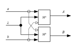
Figure 4.3: Simulation with two FPSMs without dependence on the remote inputs

Proposition.

If $p^{\mathfrak{a}}$ is not dependent on selection input $b$ and $p^{\mathfrak{b}}$ is not dependent on selection input $a$, i.e.,

$$p^{\mathfrak{a}}(A,t^{\mathfrak{a}}\mid a,b,\lambda,s^{\mathfrak{a}})=p^{\mathfrak{a}}(A,t^{\mathfrak{a}}\mid a,0,\lambda,s^{\mathfrak{a}})=p^{\mathfrak{a}}(A,t^{\mathfrak{a}}\mid a,1,\lambda,s^{\mathfrak{a}})$$

$$p^{\mathfrak{b}}(B,t^{\mathfrak{b}}\mid a,b,\lambda,s^{\mathfrak{b}})=p^{\mathfrak{b}}(B,t^{\mathfrak{b}}\mid 0,b,\lambda,s^{\mathfrak{b}})=p^{\mathfrak{b}}(B,t^{\mathfrak{b}}\mid 1,b,\lambda,s^{\mathfrak{b}})$$

for all $A,B\in\{-1,1\}$; $a,b\in\{0,1\}$; $\lambda\in\varLambda$;$s^{\mathfrak{a}},t^{\mathfrak{a}}\in S^{\mathfrak{a}};s^{\mathfrak{b}},t^{\mathfrak{b}}\in S^{\mathfrak{b}}$, then the Bell-CHSH expression will fulfill the Bell-CHSH inequality

$$\bigl{\langle}AB\bigr{\rangle}\mid_{0,0}+\bigl{\langle}AB\bigr{\rangle}\mid_{0,1}+\bigl{\langle}AB\bigr{\rangle}\mid_{1,0}-\bigl{\langle}AB\bigr{\rangle}\mid_{1,1}\;\leq\,2\textrm{.}$$

Proof.

For the conditional expectation we can write

$$\bigl{\langle}AB\bigr{\rangle}\mid_{a,b}=\sum_{\lambda\in\varLambda}\sum_{s^{\mathfrak{a}}\in S^{\mathfrak{a}}}\sum_{s^{\mathfrak{b}}\in S^{\mathfrak{b}}}p_{\Lambda}(\lambda)p_{0}^{\mathfrak{a}}(s^{\mathfrak{a}})p_{0}^{\mathfrak{b}}(s^{\mathfrak{b}})\bigl{\langle}AB\bigr{\rangle}_{a,b,\lambda,s^{\mathfrak{a}},s^{\mathfrak{b}}}$$

with

$$\bigl{\langle}AB\bigr{\rangle}_{a,b,\lambda,s^{\mathfrak{a}},s^{\mathfrak{b}}}=\sum_{A,B\in\{-1,1\}}\sum_{t^{\mathfrak{a}}\in S^{\mathfrak{a}}}\sum_{t^{\mathfrak{b}}\in S^{\mathfrak{b}}}AB\cdot p^{\mathfrak{a}}(A,t^{\mathfrak{a}}\mid a,0,\lambda,s^{\mathfrak{a}})p^{\mathfrak{b}}(B,t^{\mathfrak{b}}\mid 0,b,\lambda,s^{\mathfrak{b}})\textrm{,}$$

which can be interpreted as the output product expectation value for fixed $a,b\in\{0,1\}$; $\lambda\in\varLambda,s^{\mathfrak{a}}\in S^{\mathfrak{a}},s^{\mathfrak{b}}\in S^{\mathfrak{b}}$. Reordering gives

$$\bigl{\langle}AB\bigr{\rangle}_{a,b,\lambda,s^{\mathfrak{a}},s^{\mathfrak{b}}}=\bigl{\langle}A\bigr{\rangle}_{a,\lambda,s^{\mathfrak{a}}}\bigl{\langle}B\bigr{\rangle}_{b,\lambda,s^{\mathfrak{b}}}$$ (4.1)

with

$$\bigl{\langle}A\bigr{\rangle}_{a,\lambda,s^{\mathfrak{a}}}=\left(\sum_{A\in\{-1,1\}}\sum_{t^{\mathfrak{a}}\in S^{\mathfrak{a}}}A\cdot p^{\mathfrak{a}}(A,t^{\mathfrak{a}}\mid a,0,\lambda,s^{\mathfrak{a}})\right)\textrm{,}$$

$$\bigl{\langle}B\bigr{\rangle}_{b,\lambda,s^{\mathfrak{b}}}=\left(\sum_{B\in\{-1,1\}}\sum_{t^{\mathfrak{b}}\in S^{\mathfrak{b}}}B\cdot p^{\mathfrak{b}}(B,t^{\mathfrak{b}}\mid 0,b,\lambda,s^{\mathfrak{b}})\right)\textrm{.}$$

These expressions are the output expectation values of $M^{\mathfrak{a}}$ and $M^{\mathfrak{b}}$ with fixed $a,\lambda,s^{\mathfrak{a}}$, respectively $b,\lambda,s^{\mathfrak{b}},$ and lie in the interval $[-1,1]$. So (according Appendix A) the absolute value of the expression

$$E_{\lambda,s^{\mathfrak{a}},s^{\mathfrak{b}}}$$

$$=\bigl{\langle}A\bigr{\rangle}_{0,\lambda,s^{\mathfrak{a}}}\bigl{\langle}B\bigr{\rangle}_{0,\lambda,s^{\mathfrak{b}}}+\bigl{\langle}A\bigr{\rangle}_{0,\lambda,s^{\mathfrak{a}}}\bigl{\langle}B\bigr{\rangle}_{1,\lambda,s^{\mathfrak{b}}}+\bigl{\langle}A\bigr{\rangle}_{1,\lambda,s^{\mathfrak{a}}}\bigl{\langle}B\bigr{\rangle}_{0,\lambda,s^{\mathfrak{b}}}-\bigl{\langle}A\bigr{\rangle}_{1,\lambda,s^{\mathfrak{a}}}\bigl{\langle}B\bigr{\rangle}_{1,\lambda,s^{\mathfrak{b}}}$$ (4.2)

will be less or equal $2$ for all $\lambda\in\varLambda,s^{\mathfrak{a}}\in S^{\mathfrak{a}},s^{\mathfrak{b}}\in S^{\mathfrak{b}}$. Hence,

$$\bigl{\langle}AB\bigr{\rangle}\mid_{0,0}+\bigl{\langle}AB\bigr{\rangle}\mid_{0,1}+\bigl{\langle}AB\bigr{\rangle}\mid_{1,0}-\bigl{\langle}AB\bigr{\rangle}\mid_{1,1}$$

$$= \bigl{|}\sum_{\lambda\in\varLambda}\sum_{s^{\mathfrak{a}}\in S^{\mathfrak{a}}}\sum_{s^{\mathfrak{b}}\in S^{\mathfrak{b}}}E_{\lambda,s^{\mathfrak{a}},s^{\mathfrak{b}}}p_{\varLambda}(\lambda)p_{0}^{\mathfrak{a}}(s^{\mathfrak{a}})p_{0}^{\mathfrak{b}}(s^{\mathfrak{b}})\bigr{|}$$

$$\leq \sum_{\lambda\in\varLambda}\sum_{s^{\mathfrak{a}}\in S^{\mathfrak{a}}}\sum_{s^{\mathfrak{b}}\in S^{\mathfrak{b}}}\bigl{|}E_{\lambda,s^{\mathfrak{a}},s^{\mathfrak{b}}}\bigr{|}p_{\varLambda}(\lambda)p_{0}^{\mathfrak{a}}(s^{\mathfrak{a}})p_{0}^{\mathfrak{b}}(s^{\mathfrak{b}})$$

$$\leq \sum_{\lambda\in\varLambda}\sum_{s^{\mathfrak{a}}\in S^{\mathfrak{a}}}\sum_{s^{\mathfrak{b}}\in S^{\mathfrak{b}}}2p_{\varLambda}(\lambda)p_{0}^{\mathfrak{a}}(s^{\mathfrak{a}})p_{0}^{\mathfrak{b}}(s^{\mathfrak{b}})=2\textrm{.}$$

∎

Example 3.

The machine functions of the FPSM pairs $(M_{1}^{\mathfrak{a}},M_{1}^{\mathfrak{b}})$ and $(M_{2}^{\mathfrak{a}},M_{2}^{\mathfrak{b}})$ in example 2 are independent of both inputs. So they fulfill the Bell-CHSH inequality.

4.4 Bell’s theorem

The validity of the Bell-CHSH inequality is a logical consequence of the functional independence of $p^{\mathfrak{a}}$ from input $b$ and $p^{\mathfrak{b}}$ from input $a$. So the violation of this inequality implies that there is some functional dependence instead:

Proposition.

For any pair of FPSMs $(M^{\mathfrak{a}},M^{\mathfrak{b}})$, defined as above, which violates the Bell-CHSH inequality in the Bell test simulation, the machine $M^{\mathfrak{a}}$ (the probabilistic machine function $p^{\mathfrak{a}}$) depends on the selection input $b$ or the machine $M^{\mathfrak{b}}$ (the probabilistic machine function $p^{\mathfrak{b}}$) depends on selection input $a$.

In this case the circuit diagram has to contain at least one of the vertical connections (dotted lines in fig. 4.3).

Example 4.

The FPSM pair $(M_{3}^{\mathfrak{a}},M_{3}^{\mathfrak{b}})$ in example 2 violates the Bell-CHSH inequality. The machine function $p_{3}^{\mathfrak{b}}=\delta_{B,1-2ab}$ depends on the input $a$.

4.5 Notes

1. The expectation values in the RHS of (4.1) depend only of one selection input $a$, respectively $b$. This has the consequence that the expression (4.2) has only four variables, instead instead of eight. So the Bell-CHSH inequality is fulfilled.

2. The proof will work even if we replace the product $p_{0}^{\mathfrak{a}}(s^{\mathfrak{a}})p_{0}^{\mathfrak{b}}(s^{\mathfrak{b}})$ with a joint probability distribution function $p_{0}^{\mathfrak{ab}}(s^{\mathfrak{a}},s^{\mathfrak{b}})$ on $S^{\mathfrak{a}}\times S^{\mathfrak{b}}$, where the initial state distributions of the two machines may be not mutually independent (this could be achieved by preprocessing of some $\lambda$-input). Also in that case, the compound FPSM

   $$M^{\mathfrak{ab}}=(\{0,1\}^{2}\times\varLambda,\{-1,1\}^{2},S^{\mathfrak{a}}\times S^{\mathfrak{b}},p_{0}^{\mathfrak{ab}},p^{\mathfrak{a}}p^{\mathfrak{b}})\textrm{.}$$

   fulfills the Bell-CHSH inequality. This shows that there is a significant difference between the entanglement of quantum states (which can lead to a violation of the Bell-CHSH inequality in a similar situation, cf. app. B) and the ordinary correlation of machine states (which cannot).

3. With some additional measure theoretic assumptions the theorem can also be proven for infinite systems. But this is more relevant for physical theories then for automata theory.

5 Conclusion

The Bell theorem for finite probabilistic sequential machines shows that some data transmission between the separated machines is necessary to reproduce the statistical results of the quantum-physical Bell test experiment. The proof is simple and transparent.

It sheds some light on the physical Bell theorem if we add some ontological hypothesis, for example: any pair of locally separated physical systems can be replaced by a pair of such machines. Then a “spooky” information transmission over distances has to be assumed to explain the experimental results (see Gisin et al. 2008).

But the automata-theoretic version of the theorem has a value in itself. It sets some limits for networks of probabilistic sequential machines that are used for the description of communication devices. These limits can be exceeded by quantum devices (cf. app. B), which empowers quantum-cryptographic protocols (e.g., Ekert, 1991).

Appendix A Bell-CHSH inequality

Proposition.

Any four real numbers $A_{0},A_{1},B_{0},B_{1}\in[-1,1]$ fulfill the Bell-CHSH inequality

$$\bigl{|}A_{0}B_{0}+A_{0}B_{1}+A_{1}B_{0}-A_{1}B_{1}\bigr{|}\leq 2\textrm{.}$$ (A.1)

Proof.

The expression

$$A_{0}B_{0}+A_{0}B_{1}+A_{1}B_{0}-A_{1}B_{1}$$

is linear in each of the four variables. So its maximum and minimum are located on a corner of the hyper-cube $[-1,1]^{{}^{4}}$with $A_{0},A_{1},B_{0},B_{1}\in\{-1,1\}$. In this case for all 16 possible valuations the following equation is valid

$$A_{0}B_{0}+A_{0}B_{1}+A_{1}B_{0}-A_{1}B_{1}=A_{0}\left(B_{0}+B_{1}\right)+A_{1}\left(B_{0}-B_{1}\right)=\pm 2\textrm{.}$$

∎

Proposition.

Four random variables $A_{0},A_{1},B_{0},B_{1}\colon\varLambda\rightarrow[-1,1]$ on a measure space $(\varLambda,\Sigma)$ fulfill for any probability measure $\mu$ on $(\varLambda,\Sigma)$ the Bell-CHSH inequality

$$\bigl{|}\bigl{\langle}A_{0}B_{0}+A_{0}B_{1}+A_{1}B_{0}-A_{1}B_{1}\bigr{\rangle}_{\mu}\bigr{|}\leq 2$$

where $\bigl{\langle}\;\bigr{\rangle}_{\mu}$indicates the expectation value with the measure $\mu$.

Proof.

Let

$$C(\lambda)=A_{0}(\lambda)B_{0}(\lambda)+A_{0}(\lambda)B_{1}(\lambda)+A_{1}(\lambda)B_{0}(\lambda)-A_{1}(\lambda)B_{1}(\lambda)\textrm{.}$$

Then because of (A.1) $\left|C(\lambda)\right|\leq 2$ for all $\lambda\in\Lambda$ and

$$\bigl{|}\bigl{\langle}C\bigr{\rangle}_{\mu}\bigr{|}=\bigl{|}\intop_{\varLambda}C(\lambda)d\mu\bigr{|}\leq\intop_{\varLambda}\bigl{|}C(\lambda)\bigr{|}d\mu\leq\intop_{\varLambda}2d\mu=2\textrm{.}$$

∎

Appendix B Example of quantum sequential machines violating Bell-CHSH inequality

A quantum sequential machine can be defined in a similar way as a probabilistic one. The essential difference is the use of complex-valued amplitude functions instead of non-negative real-valued probability distribution functions. Calculations with these amplitudes are performed in very a similar way as with probabilities. At the end of the calculation the absolute (modulus) square of the resulting amplitude gives the probability.

We define a finite quantum SM (FQSM) as a quintuple $(I,O,S,\psi_{0},\varphi)$, where $I,O,S$ are finite sets of input symbols, output symbols and states,

$$\psi_{0}\colon S\rightarrow\mathbb{C},s\mapsto\psi_{0}(s)$$

is the initial state amplitude function with

$$\sum_{s\in S}\bigl{|}\psi_{0}(s)\bigr{|}^{2}=1\textrm{,}$$

and

$$\varphi\colon O\times S\times I\times S\rightarrow\mathbb{C},(o,t,i,s)\mapsto\varphi(o,t|i,s)$$

is the quantum machine function with

$$\sum_{o\in O}\sum_{t\in S}\bigl{|}\sum_{s\in S}\varphi(o,t|i,s)\psi_{0}(s)\bigr{|}^{2}=1$$

for all $i\in I,s\in S$.

The probability to get the output $o$ and the new state $t$ after the input $i$ in the initial state with amplitude $\psi_{0}$ is

$$\bigl{|}\sum_{s\in S}\varphi(o,t|i,s)\psi_{0}(s)\bigr{|}^{2}\textrm{.}$$

Example 5.

Our example is a pair $(Q^{\mathfrak{a}},Q^{\mathfrak{b}})$ of FQSMs that violates the Bell-CHSH inequality without dependence on the remote input if it is initialized with a non-product initial state amplitude function.

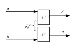
Figure B.1: Simulation of the Bell experiment with two FQSMs with entangled initial state amplitude function

Both machines have the input set $I=\{0,1\}$ and the output set $O=\{-1,1\}$. The state set is $S=\{0,1\}$—so both machines are essentially qubits. The FQSMs have the form

$$Q^{\mathfrak{a}}=(\{0,1\},\{-1,1\},\{0,1\},\psi_{0}^{\mathfrak{a}},\varphi^{\mathfrak{a}})\textrm{,}$$

$$Q^{\mathfrak{b}}=(\{0,1\},\{-1,1\},\{0,1\},\psi_{0}^{\mathfrak{b}},\varphi^{\mathfrak{b}}).$$

The quantum machine functions $\varphi^{\mathfrak{a}}$, $\varphi^{\mathfrak{b}}$ are (in table form):

$\varphi^{\mathfrak{a}}$	$a=0$, $s^{\mathfrak{a}}=0$	$a=0$, $s^{\mathfrak{a}}=1$	$a=1$, $s^{\mathfrak{a}}=0$	$a=1$, $s^{\mathfrak{a}}=1$
$t^{\mathfrak{a}}=0$, $A=-1$	$1$	$0$	$\frac{1}{\sqrt{2}}$	$\frac{1}{\sqrt{2}}$
$t^{\mathfrak{a}}=1$, $A=1$	0	1	$\frac{1}{\sqrt{2}}$	$-\frac{1}{\sqrt{2}}$

$\varphi^{\mathfrak{b}}$	$a=0$, $s^{\mathfrak{b}}=0$	$a=0$, $s^{\mathfrak{b}}=1$	$a=1$, $s^{\mathfrak{b}}=0$	$a=1$, $s^{\mathfrak{b}}=1$
$t^{\mathfrak{b}}=0$, $A=-1$	$-\frac{1}{\sqrt{4+2\sqrt{2}}}$	$\frac{1+\sqrt{2}}{\sqrt{4+2\sqrt{2}}}$	$\frac{1}{\sqrt{4+2\sqrt{2}}}$	$\frac{1+\sqrt{2}}{\sqrt{4+2\sqrt{2}}}$
$t^{\mathfrak{b}}=1$, $A=1$	$\frac{1+\sqrt{2}}{\sqrt{4+2\sqrt{2}}}$	$\frac{1}{\sqrt{4+2\sqrt{2}}}$	$-\frac{1+\sqrt{2}}{\sqrt{4+2\sqrt{2}}}$	$\frac{1}{\sqrt{4+2\sqrt{2}}}$

Both machines are Moore machines where the new state $t^{\mathfrak{a}}$, respectively $t^{\mathfrak{b}}$, determines the output (i.e., $A=2t^{\mathfrak{a}}-1$, $B=2t^{\mathfrak{b}}-1$). We omitted rows which contain zeros only (e.g., $t^{\mathfrak{a}}=0,$ $A=1$).

The conditional output expectation is

$$\bigl{\langle}AB\bigr{\rangle}\mid_{a,b}=\sum_{A\in\{-1,1\}}\sum_{B\in\{-1,1\}}AB\cdot q\left(A,B\mid a,b\right)$$

with the conditional probability to get the output $(A,B)$ after input $(a,b)$

$$q\left(A,B\mid a,b\right)=$$

$$\bigl{|}\sum_{s^{\mathfrak{a}}\in\{0,1\}}\sum_{s^{\mathfrak{b}}\in\{0,1\}}\sum_{t^{\mathfrak{a}}\in\{0,1\}}\sum_{t^{\mathfrak{b}}\in\{0,1\}}\varphi^{\mathfrak{a}}(A,t^{\mathfrak{a}}\mid a,s^{\mathfrak{a}})\varphi^{\mathfrak{b}}(B,t^{\mathfrak{b}}\mid b,s^{\mathfrak{b}})\psi_{0}^{\mathfrak{a}}(s^{\mathfrak{a}})\psi_{0}^{\mathfrak{b}}(s^{\mathfrak{b}})\bigr{|}^{2}\textrm{.}$$

However, to violate the Bell-CHSH inequality, the product $\psi_{0}^{\mathfrak{a}}(s^{\mathfrak{a}})\psi_{0}^{\mathfrak{b}}(s^{\mathfrak{b}})$ has to be replaced with a non-product (i.e., entangled) initial state amplitude function

$$\psi_{0}^{\mathfrak{ab}}(s^{\mathfrak{a}},s^{\mathfrak{b}})=\frac{1}{\sqrt{2}}(\delta_{s^{\mathfrak{a}},0}\delta_{s^{\mathfrak{b}},1}-\delta_{s^{\mathfrak{a}},1}\delta_{s^{\mathfrak{b}},0})\textrm{.}$$

In this case the compound FQSM

$$Q^{\mathfrak{ab}}=(\{0,1\}^{2},\{-1,1\}^{2},\{0,1\}^{2},\psi_{0}^{\mathfrak{ab}},\varphi^{\mathfrak{a}}\varphi^{\mathfrak{b}})$$

gives the following conditional output probability (in table form):

$q\left(A,B\mid a,b\right)$	$a,b=0,0$	$a,b=0,1$	$a,b=1,0$	$a,b=1,1$
$A,B=(-1,-1)$	$\frac{2+\sqrt{2}}{8}$	$\frac{2+\sqrt{2}}{8}$	$\frac{2+\sqrt{2}}{8}$	$\frac{2-\sqrt{2}}{8}$
$A,B=(-1,1)$	$\frac{2-\sqrt{2}}{8}$	$\frac{2-\sqrt{2}}{8}$	$\frac{2-\sqrt{2}}{8}$	$\frac{2+\sqrt{2}}{8}$
$A,B=(1,-1)$	$\frac{2-\sqrt{2}}{8}$	$\frac{2-\sqrt{2}}{8}$	$\frac{2-\sqrt{2}}{8}$	$\frac{2+\sqrt{2}}{8}$
$A,B=(1,1)$	$\frac{2+\sqrt{2}}{8}$	$\frac{2+\sqrt{2}}{8}$	$\frac{2+\sqrt{2}}{8}$	$\frac{2-\sqrt{2}}{8}$

This is identical with

$$q_{5}\left(A,B\mid a,b\right)=\frac{2-\sqrt{2}}{8}+\frac{\sqrt{2}}{8}(2\delta_{A,B}+2ab-4ab\delta_{A,B})$$

from FPSM $M_{5}$ in example 1 and gives the Tsirelson bound $2\sqrt{2}$ as expectation value of the Bell-CHSH expression.

References

• Aspect et al. [1982] A. Aspect, J. Dalibard, and G. Roger. Experimental test of Bell’s inequalities using time-varying analyzers. Phys. Rev. Lett., 49, 1982. doi: 10.1103/PhysRevLett.49.91.
• Bell [1964] J. S. Bell. On the Einstein-Podolsky-Rosen paradox. Physics, 1, 1964. doi: 10.1017/CBO9780511815676.004.
• Bell [1981] J. S. Bell. Bertlmann’s socks and the nature of reality. Journal de Physique, 42, 1981. doi: 10.1017/CBO9780511815676.018.
• Bohm [1951] D. Bohm. Quantum Theory. Prentice-Hall, Inc., 1951.
• Cirel’son [1980] B. S. Cirel’son. Quantum Generalizations of Bell’s Inequality. Lett. Math. Phys., 4, 1980. doi: 10.1007/BF00417500.
• Clauser et al. [1969] J. F. Clauser, M. A. Horne, A. Shimony, and R. A. Holt. Proposed experiment to test local hidden-variable theories. Phys. Rev. Lett., 23, 1969. doi: 10.1103/PhysRevLett.23.880.
• Einstein et al. [1935] A. Einstein, B. Podolsky, and N. Rosen. Can quantum-mechanical description of physical reality be considered complete? Phys. Rev., 47, 1935. doi: 10.1103/PhysRev.47.777.
• Ekert [1991] A. K. Ekert. Quantum cryptography based on Bell’s theorem. Phys. Rev. Lett., 67, 1991. doi: 10.1103/PhysRevLett.67.661.
• Gill [2014] R. Gill. Statistics, Causality and Bell’s Theorem. arXiv:1207.5103, 2014.
• Gisin et al. [2008] N. Gisin, D. Salart, A. Baas, C. Branciard, and H. Zbinden. Testing spooky action at a distance. Nature, 454, 2008. doi: 10.1038/nature07121.
• Salomaa [1969] A. Salomaa. Theory of Automata. Pergamon Press, Oxford, 1969.
• Say and Yakaryilmaz [2014] A. C. C. Say and A. Yakaryilmaz. Quantum finite automata: A modern introduction. LNCS 8808, arXiv:1406.4048v1[cs.FL], 2014.
• Shimony [2016] A. Shimony. Bell’s theorem. In E. N. Zalta, editor, The Stanford Encyclopedia of Philosophy. Metaphysics Research Lab, Stanford University, 2016. URL https://plato.stanford.edu/archives/win2016/entries/bell-theorem/.
• Stapp [1975] H. P. Stapp. Bell’s theorem and world process. Nuovo Cimento., 29B, 1975. doi: 10.1007/BF02728310.