Combined parametrization of $G_{En}$ and $\gamma^{\ast}N\to\Delta(1232)$
quadrupole form factors

Abstract

Models based on $SU(6)$ symmetry breaking and large $N_{c}$ limit provide relations between the pion cloud contributions to the $\gamma^{\ast}N\to\Delta(1232)$ quadrupole form factors, electric ($G_{E}$) and Coulomb ($G_{C}$), and the neutron electric form factor $G_{En}$, suggesting that those form factors are dominated by the same physical processes. Those relations are improved in order to satisfy a fundamental constraint between the electric and Coulomb quadrupole form factors in the long wavelength limit, when the photon three-momentum vanishes (Siegert’s theorem). Inspired by those relations, we study alternative parametrizations for the neutron electric form factor. The parameters of the new form are then determined by a combined fit to the $G_{En}$ and the $\gamma^{\ast}N\to\Delta(1232)$ quadrupole form factor data. We obtain a very good description of the $G_{E}$ and $G_{C}$ data when we combine the pion cloud contributions with small valence quark contributions to the $\gamma^{\ast}N\to\Delta(1232)$ quadrupole form factors. The best description of the data is obtained when the second momentum of $G_{En}$ is $r_{n}^{4}\simeq-0.4$ fm⁴. We conclude that the square radii associated with $G_{E}$ and $G_{C}$, $r_{E}^{2}$ and $r_{C}^{2}$, respectively, are large, revealing the long extension of the pion cloud. We conclude also that those square radii are related by $r_{E}^{2}-r_{C}^{2}=0.6\pm 0.2$ fm². The last result is mainly the consequence of the pion cloud effects and Siegert’s theorem.

1 Introduction

Among all the nucleon excitations the $\Delta(1232)$ plays a special rule, not only because it is a spin 3/2 system with the same quark content as the nucleon, but also because it is very well known experimentally NSTAR ; Pascalutsa07b ; Aznauryan12b . The electromagnetic transition between the nucleon ($N$) and the $\Delta(1232)$ is characterized by the magnetic dipole form factor ($G_{M}$) and two quadrupole form factors: the electric ($G_{E}$) and the Coulomb ($G_{C}$) form factors Jones73 . The magnetic dipole is the dominant form factor, as expected from the quark spin-flip transition Beg64 ; Becchi65 ; JDiaz07 ; NDelta ; Lattice ; OctetDecuplet1 ; OctetDecuplet2 ; Eichmann12 ; Segovia13 ; SAlepuz17 , while the quadrupole form factors are small, but non-zero NSTAR ; Pascalutsa07b ; Isgur82 ; Capstick90 ; NDeltaD ; LatticeD ; Siegert-ND ; Letter . The transition form factors are traditionally represented in terms of $Q^{2}=-q^{2}$, where $q$ is the $\gamma^{\ast}N\to\Delta(1232)$ momentum transfer, or photon momentum. Experimental data are available only in the region $Q^{2}\geq 0$.

The non-zero results for the quadrupole form factors are the consequence of asymmetries on the $\Delta(1232)$ structure, which implies the deviation of the $\Delta(1232)$ from a spherical shape Pascalutsa07b ; Becchi65 ; Capstick90 ; Glashow79 ; Bernstein03 ; Buchmann97a ; Krivoruchenko91 ; Buchmann00b ; Deformation ; Quadrupole1 ; Quadrupole2 . Estimates of the electric and Coulomb quadrupole form factors based on valence quark degrees of freedom can explain in general only a small fraction of the observed data Pascalutsa07b ; Becchi65 ; JDiaz07 ; Capstick90 ; Buchmann00b ; Tiator04 ; Kamalov99 ; Kamalov01 ; SatoLee . The strength, missing in quark models can be explained when we take into account the quark-antiquark effects in the form of meson cloud contributions Tiator04 ; Kamalov99 ; Kamalov01 ; SatoLee ; Pascalutsa07a ; QpionCloud1 ; QpionCloud2 ; NSTAR2017 .

Calculations based on non relativistic $SU(6)$ quark models with symmetry breaking and large $N_{c}$ limit show that the $\gamma^{\ast}N\to\Delta(1232)$ quadrupole form factors are dominated by pion cloud effects at small $Q^{2}$ ($Q^{2}<1$ GeV²) Pascalutsa07b ; Buchmann97a ; Pascalutsa07a ; Buchmann04 ; Grabmayr01 ; Buchmann09a ; Buchmann02 . Simple parametrizations of the pion cloud contributions to the quadrupole form factors $G_{E}$ and $G_{C}$, labeled as $G_{E}^{\pi}$ and $G_{C}^{\pi}$, respectively, have been derived using the large $N_{c}$ limit Pascalutsa07a , in close agreement with the empirical data Pascalutsa07a ; Blomberg16a . Those parametrizations relate $G_{E}^{\pi}$ and $G_{C}^{\pi}$ with the neutron electric form factor Pascalutsa07a ; Grabmayr01 ; Buchmann09a , and are discussed in sect. 2.

There are some limitations associated with the use of those pion cloud parametrizations: they underestimate the $Q^{2}<0.2$ GeV² data by about 10-20% Siegert-ND ; Letter ; Blomberg16a ; SiegertD , and they are in conflict with Siegert’s theorem, a fundamental constraint between the quadrupole form factors also known as the long wavelength limit Siegert-ND ; Letter ; Buchmann98 ; Drechsel2007 ; Tiator1 ; Tiator2 .

Siegert’s theorem states that at the pseudothreshold, when $Q^{2}=Q^{2}_{pt}\equiv-(M_{\Delta}-M)^{2}$, one has Jones73 ; Siegert-ND ; Letter ; SiegertD ; Siegert

$$G_{E}(Q_{pt}^{2})=\kappa G_{C}(Q^{2}_{pt}),$$ (1)

where $M$ and $M_{\Delta}$ are the nucleon and $\Delta(1232)$ masses, respectively, and $\kappa={\textstyle\frac{M_{\Delta}-M}{2M_{\Delta}}}$. The pseudothreshold is the point where the photon three-momentum ${\bf q}$, vanishes ($|{\bf q}|=0$), and the nucleon and the $\Delta(1232)$ are both at rest.

Concerning Siegert’s theorem, the problem can be sol-ved correcting the parametrization for $G_{E}^{\pi}$ with a term ${\cal O}(1/N_{c}^{2})$ at the pseudothreshold, as shown recently in Letter . Concerning the underestimation of the data associated with the quadrupole form factors $G_{E}$ and $G_{C}$, it can be partially solved with the addition of contributions to those form factors associated with the valence quarks. Although small, those contributions move the estimates based on the pion cloud effects in the direction of the measured data JDiaz07 ; LatticeD ; Siegert-ND ; Kamalov99 ; Kamalov01 .

In the previous picture, there is only a small setback, the combination of pion cloud and valence quark contributions is unable to describe the previous Coulomb quadrupole form factor data below 0.2 GeV² Siegert-ND . However, it has been shown recently that the previous extractions of $G_{C}$ data at low $Q^{2}$ ($Q^{2}<0.2$ GeV²) overestimate the actual values of the form factor Blomberg16a , and that the new results are in excellent agreement with the estimates based on the pion cloud parametrizations Letter .

The main motivation for this work is to check if there are parametrizations of $G_{En}$ which optimizes the description of the $G_{E}$ and $G_{C}$ data and provides at the same time an accurate description of the neutron electric form factor data. With this goal in mind, we perform a global fit of the functions $G_{En}$, $G_{E}^{\pi}$ and $G_{C}^{\pi}$, to the experimental form factor data, based on the pion cloud parametrization of the quadrupole form factors. An accurate description of the data indicates a correlation between the pion cloud effects in the neutron and in the $\gamma^{\ast}N\to\Delta(1232)$ transition Pascalutsa07a . In addition, a global fit, which includes the $G_{E}$ and $G_{C}$ data, can help to constrain the shape of $G_{En}$, since the neutron electric form factor data have in general large error bars.

The main focus of the present work is then on the parametrization of the function $G_{En}$. In the past, simplified parametrizations of $G_{En}$ with a small number of parameters have been used. Examples of these parametrizations, are, the Galster parametrization, and the Bertozzi parametrization, based on the differences of two poles, among others Galster71 ; Kelly02 ; Friedrich03 ; Bertozzi72 ; Platchkov90 ; Kaskulov04 ; Gentile11 . More sophisticated parametrizations, with a larger number of parameters have been derived based on dispersion relations and chiral perturbation theory Kaiser03 ; Belushkin07 ; Hammer04 ; Lorenz12 . For the purpose of the present work, however, it is preferable to use simple expressions with a small number of parameters. We propose then a parametrization of $G_{En}$ with three parameters.

The parametrizations of $G_{En}$ can also be analyzed in terms of first moments of the expansion of $G_{En}$ near $Q^{2}=0$, namely, the first ($r_{n}^{2}$), the second ($r_{n}^{4}$) and the third ($r_{n}^{6}$) moments. The explicit definitions are presented in sect. 3. In the present work, motivated by a previous study of the $\gamma^{\ast}N\to\Delta(1232)$ quadrupole form factors and their relations with Siegert’s theorem Siegert-ND , we consider a parametrization of $G_{En}$ based on rational functions. Those parametrizations have a simple form for low $Q^{2}$ and are also compatible with the expected falloff at large $Q^{2}$. Alternative parametrizations based on rational functions can be found in Siegert-ND ; ComptonScattering .

As mentioned above, the description of the $G_{E}$ and $G_{C}$ data can be improved when we include additional contributions associated with the valence quark component. Inspired by previous works, where the valence quark contributions are estimated based on the analysis of the results from lattice QCD Lattice ; LatticeD ; Siegert-ND , we include in the present study the valence quark contributions calculated with the covariant spectator quark model from LatticeD . The model under discussion is covariant and consistent with lattice QCD results NDelta ; LatticeD ; Nucleon . Since in lattice QCD simulations with large pion masses the meson contributions are suppressed, the physics associated with the valence quarks can be calibrated more accurately within the model uncertainties Lattice . An additional advantage in the use of a quark model framework is that the $G_{E}$ and $G_{C}$ form factors are identically zero at the pseudothreshold, as a consequence of the orthogonality between the nucleon and $\Delta(1232)$ states LatticeD ; Siegert-ND . This point is fundamental for the consistence of the present model with the constraints of Siegert’s theorem.

We conclude at the end, that the combination of the $G_{En}$, $G_{E}$ and $G_{C}$ data does help to improve the accuracy of the parametrization of $G_{En}$ (small errors associated with the parameters). The best description of the data is obtained when the second moment of $G_{En}$, $r_{n}^{4}$ is about $-0.38$ fm⁴. A consequence of this result is that the square radii associated with $G_{E}$ and $G_{C}$ ($r_{E}^{2}$ and $r_{C}^{2}$) are large, suggesting a long spacial extension of the pion cloud (or quark-antiquark distribution) for both form factors. We conclude also that, as a consequence of the pion cloud parametrizations of the $G_{E}$ and $G_{C}$ quadrupole form factors, one obtains $r_{E}^{2}-r_{C}^{2}=0.6\pm 0.2$ fm². The uncertainties of the estimates are also discussed.

This article is organized as follows: In the next section, we discuss the pion cloud parametrizations of the $\gamma^{\ast}N\to\Delta(1232)$ quadrupole form factors. In sect. 3, we discuss our parametrization of the neutron electric form factor. In sect. 4, we present the results of the global fit to the $G_{En}$, $G_{E}$ and $G_{C}$ data, and discuss the physical consequences of the results. The outlook and conclusions are presented in sect. 5.

2 Pion cloud parametrization of $G_{E}$ and $G_{C}$

The internal structure of the baryons can be described using a combination $SU(6)$ quark models with two-body exchange currents and the large $N_{c}$ limit Buchmann04 ; Grabmayr01 ; Buchmann09a . The $SU(6)$ symmetry breaking induces an asymmetric distribution of charge in the nucleon and $\Delta(1232)$ systems, which is responsible for the non-vanishment of the neutron electric form factor and for the non-zero results for the $\gamma^{\ast}N\to\Delta(1232)$ quadrupole moments Buchmann09a . Those results can be derived in the context of constituent quark models as the Isgur-Karl model Isgur81a ; IsgurRefs1 ; IsgurRefs2 , and others Pascalutsa07b ; Buchmann97a ; Grabmayr01 . More specifically, we can conclude, based on the $SU(6)$ symmetry breaking, that the $\gamma^{\ast}N\to\Delta(1232)$ quadrupole moments are proportional to the neutron electric square radius ($r_{n}^{2}$). Based on similar arguments, we can also relate the electric quadrupole moment of the $\Delta(1232)$ and other baryons, with the neutron electric square radius Buchmann97a ; Krivoruchenko91 ; Buchmann02 ; Dillon99 ; Buchmann02b ; Buchmann00a . From the large $N_{c}$ framework, we can conclude that when $Q^{2}=0$, one has ${\textstyle\frac{G_{E}}{G_{M}}}={\cal O}({\textstyle\frac{1}{N_{c}^{2}}})$ and $G_{E}={\textstyle\frac{M_{\Delta}^{2}-M^{2}}{4M_{\Delta}^{2}}}G_{C}$ Pascalutsa07b ; Jenkins02 .

The derivation of the pion cloud contribution to the $\gamma^{\ast}N\to\Delta(1232)$ quadrupole form factors are based on relations between the quadrupole moments and the neutron electric square radius, discussed above, and on the low-$Q^{2}$ expansion of the neutron electric form factor: $G_{En}\simeq-{\textstyle\frac{1}{6}}r_{n}^{2}Q^{2}$ Buchmann97a ; Pascalutsa07a ; Buchmann04 ; Grabmayr01 ; Buchmann09a ; Buchmann02 . One can then write

$$G_{E}^{\pi}(Q^{2})=\left(\frac{M}{M_{\Delta}}\right)^{3/2}\frac{M_{\Delta}^{2}-M^{2}}{2\sqrt{2}}\frac{\tilde{G}_{En}(Q^{2})}{1+\frac{Q^{2}}{2M_{\Delta}(M_{\Delta}-M)}},$$ (2)

$$G_{C}^{\pi}(Q^{2})=\left(\frac{M}{M_{\Delta}}\right)^{1/2}\sqrt{2}M_{\Delta}M\tilde{G}_{En}(Q^{2}),$$ (3)

where $\tilde{G}_{En}=G_{En}/Q^{2}$.

The interpretation of the previous relations as representative of the pion cloud contributions is a consequence of the connection between quadrupole form factors and $r_{n}^{2}$. Those relations have been derived in the framework of the constituent form factors with two-body exchange currents. The effects of those currents can be interpreted as pion/meson contributions since they include processes associated with pion exchange and quark-antiquark pairs Buchmann04 ; Grabmayr01 ; Buchmann09a ; Buchmann02 . This interpretation is also valid in the large $N_{c}$ limit, where the form factor $G_{E}$ and the product $\frac{|{\bf q}|}{2M_{\Delta}}G_{C}$ appear as higher orders in $1/N_{c}$ compared to $G_{M}$ Pascalutsa07a ; Jenkins02 .

For future discussions, it is worth noticing that the $SU(6)$/large$N_{c}$ estimates are based on non relativistic kinematics and therefore may ignore some high angular momentum state effects that emerge in a relativistic framework.

Indications of the dominance of the pion cloud contributions have been found also within the framework of the dynamical coupled-channel models, like the Sato-Lee and the DMT models JDiaz07 ; Kamalov99 ; Kamalov01 ; SatoLee ; Blomberg16a .

It is worth mentioning that eqs. (2)-(3) should not be strictly interpreted as pion cloud contributions, because the empirical parametrization of $G_{En}$ include all possible contributions, including also the effects of the valence quarks. We note, however, that in an exact $SU(6)$ model the contributions from the valence quarks associated with one-body currents vanishes Buchmann09a ; Dillon99 ; Lichtenberg78 ; Close89 . In a model where the $SU(6)$ symmetry is broken in first approximation, one can expect that the quark-antiquark contributions are the dominant effect in $G_{En}$ and $r_{n}^{2}$ Grabmayr01 ; Buchmann09a . Examples of models with meson cloud/sea quark dominance can be found in Buchmann00b ; Buchmann97a ; Buchmann91 ; Christov96 ; Lu98 . We conclude then that (2)-(3) can still be used to estimate the pion cloud contribution to the $\gamma^{\ast}N\to\Delta(1232)$ quadrupole form factors in the cases where the valence quark contributions are small.

We assume that eqs. (2)-(3) and in particular the analytic parametrizations of $G_{En}$ hold also for $Q^{2}<0$. This assumption is justified by the smooth behavior inferred for $G_{En}$ based on the empirical data, and also because the range of extrapolation is small, since $Q_{pt}^{2}\simeq-0.086$ GeV². In this range, the effects associated with the timelike pole structure, such as the effects of the $\rho$-pole ($Q^{2}\simeq-0.6$ GeV²), are attenuated, or can be represented in an effective form. In sect. 4.5 we show that $G_{En}$ is in fact dominated, near the pseudothreshold, by the first two terms of the expansion in $Q^{2}$. Note that the two pion production threshold $Q^{2}=-4m_{\pi}^{2}\simeq-0.076$ GeV², the point where the transition form factors become complex functions, is just a bit above the $\gamma^{\ast}N\to\Delta(1232)$ pseudothreshold. Since, according to chiral perturbation theory, the transition to the complex form factors is smooth Kaiser03 ; Belushkin07 , we can ignore the imaginary component of the form factors in first approximation, and treat the form factors in the timelike region as simple extrapolations of the analytic parametrizations derived in the spacelike region. Similar extrapolations to the timelike region can also be found in Drechsel2007 ; Tiator07 ; Tiator11 .

The relations (2)-(3) are derived in Letter and improve previous large $N_{c}$ relations Pascalutsa07a , in order to satisfy Siegert’s theorem exactly (1). The main difference between our analytic expressions for the functions $G_{E}^{\pi}$ and $G_{C}^{\pi}$ compared to the expressions derived in Pascalutsa07a , is in eq. (2), where we include a denominator in the factor $\tilde{G}_{En}$. This new factor corresponds to a relative correction ${\cal O}(1/N_{c}^{2})$, relative to the original derivation for $G_{E}^{\pi}$, at the pseudothreshold. Using the new form, one obtains at the pseudothreshold: $1+{\textstyle\frac{Q^{2}}{2M_{\Delta}(M_{\Delta}-M)}}={\textstyle\frac{M_{\Delta}+M}{2M_{\Delta}}}$, which lead directly to eq. (1). In a previous work Siegert-ND , an approximated expression was considered for $G_{E}^{\pi}$, where the error in the description of Siegert’s theorem is a term ${\cal O}(1/N_{c}^{4})$.

Previous studies of Siegert’s theorem based on quark models Capstick90 ; Buchmann98 ; Drechsel84 ; Weyrauch86 ; Bourdeau87 show that the theorem can be violated when the operators associated with the charge density, or the current density, are truncated in different orders, inducing a violation of the current conservation condition Buchmann98 . From those works, we can conclude that, a consistent calculation with current conservation, cannot be reduced to the photon coupling with the individual quarks (one-body currents), since the current is truncated. In those conditions, it is necessary the inclusion of higher-order terms such as two-body currents, in order to ensure current conservation and to be consistent with Siegert’s theorem Buchmann98 . The description of Siegert’s theorem, requires then the inclusion of processes beyond the impulse approximation (one-body currents) SiegertD ; Buchmann98 .

We recall at this point that eqs. (2)-(3) are the result of derivations valid at small $Q^{2}$ Pascalutsa07a . For very large values of $Q^{2}$, we expect the pion cloud contributions to be negligible in comparison to the valence quark contributions. Thus, one can assume that for large $Q^{2}$, the equations (2)-(3) are corrected according to $G_{E}^{\pi}\to G_{E}^{\pi}/(1+Q^{2}/\Lambda_{E}^{2})^{2}$ and $G_{C}^{\pi}\to G_{C}^{\pi}/(1+Q^{2}/\Lambda_{C}^{2})^{4}$, where $\Lambda_{E}$ and $\Lambda_{C}$ are large momentum cutoff parameters Letter . In those conditions, the form factors $G_{E}$ and $G_{C}$ are, at large $Q^{2}$, dominated by the valence quark contributions, as predicted by perturbative QCD, with falloffs $G_{E}\propto 1/Q^{4}$ and $G_{C}\propto 1/Q^{6}$ Carlson1 ; Carlson2 . The falloffs of the pion cloud components are then $G_{E}^{\pi}\propto 1/Q^{8}$ and $G_{C}^{\pi}\propto 1/Q^{10}$, where the extra factor ($1/Q^{4}$) takes into account the effect of the extra quark-antiquark pair associated with the pion cloud Carlson1 ; Carlson2 .

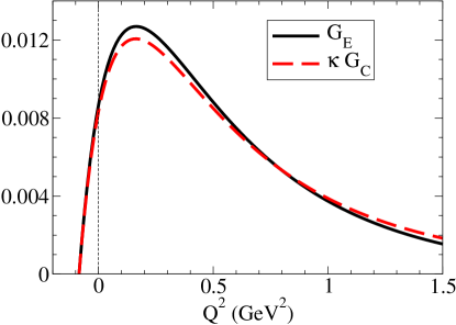
Figure 1: Valence quark contributions for $G_{E}$ and $G_{C}$ according to LatticeD . Recall that $\kappa={\textstyle\frac{M_{\Delta}-M}{2M_{\Delta}}}\simeq 0.12$.

Adding the valence quark contributions

The pion cloud contributions to the $\gamma^{\ast}N\to\Delta(1232)$ quadrupole form factors given by eqs. (2)-(3) should be complemented by valence quark contributions to the respective form factors. Calculations from quark models estimate that the valence quark contribution to the $\gamma^{\ast}N\to\Delta(1232)$ quadrupole form factors are an order of magnitude smaller than the data NSTAR ; JDiaz07 ; Capstick90 ; NDeltaD ; NSTAR2017 ; Stave08 . It is known, however, that small valence quark contributions to the quadrupole form factors can help to improve the description of the data LatticeD ; Siegert-ND .

The valence quark contributions to the $\gamma^{\ast}N\to\Delta(1232)$ quadrupole form factors are in general the result of high angular momentum components in the nucleon and/or $\Delta(1232)$ wave functions. The valence quark contributions to the quadrupole form factors vanish at the pseudothreshold, as a consequence of the orthogonality between the nucleon and $\Delta(1232)$ states, as discussed in Siegert-ND . In those conditions, the valence quark contributions to the quadru-pole form factors play no role in Siegert’s theorem, which depends exclusively on the pion cloud contributions. The parameterizations (2)-(3) then ensure that Siegert’s theorem is naturally satisfied.

In order to improve the description of the $\gamma^{\ast}N\to\Delta(1232)$ quadrupole form factors, we combine the pion cloud parametrizations (2)-(3) with the valence quark contributions (index B), using $G_{a}=G_{a}^{\rm B}+G_{a}^{\pi}$, for $a=E,C$. For the valence quark contributions we use in particular the quark model from LatticeD , since in this work the valence quark contributions are calculated using an extrapolation from the lattice QCD simulations in the quenched approximation with large pion masses Alexandrou08 . Recall that in lattice QCD simulations with large pion masses, the meson cloud effects are very small, and the physics associated with the valence quarks can be better calibrated Lattice ; LatticeD ; Omega . The free parameters of the model are two $D$-state admixture coefficients and three momentum scales associated with the radial structure of the $D$-states. All those parameters are determined accurately by the results from lattice QCD simulations LatticeD . The chi-square per degree of freedom associated with the fit of the model to the lattice QCD results is 0.58 for $G_{E}$ and $1.17$ for $G_{C}$. The number of degrees of freedom of the fit is 37 and the combined chi-square per degree of freedom is 0.76.

The model under discussion is covariant and can therefore be used to estimate the valence quark contributions in any range of $Q^{2}$ LatticeD ; Nucleon . The results of the valence quark contributions to the form factors $G_{E}$ and $G_{C}$ estimated by the model from LatticeD are presented in fig. 1. The available data near $Q^{2}=0$ is $G_{E}(0)=0.076\pm 0.015$ and $\kappa G_{C}(0.04\;\mbox{GeV}^{2})=0.075\pm 0.021$ Letter ; Blomberg16a ; PDG . Based on fig. 1, one can then conclude that the valence quarks contribute only for about 10% of the empirical data near $Q^{2}=0$. The theoretical uncertainties associated with the results from fig. 1 are discussed later on.

Estimates based on the Dyson-Schwinger formalism suggest that relativistic effects, in particular $P$-state contributions, can increase the magnitude of the valence quark contributions Eichmann12 ; Segovia13 . These results suggest that our estimates of the pion cloud contributions may be overestimated.

3 Parametrizations of $G_{En}$

The parametrizations of $G_{En}$ can be represented by an expansion near $Q^{2}=0$ in the form Grabmayr01 :

$$G_{En}(Q^{2})\simeq-{\textstyle\frac{1}{6}}r_{n}^{2}Q^{2}+{\textstyle\frac{1}{120}}r_{n}^{4}Q^{4}-{\textstyle\frac{1}{5040}}r_{n}^{6}Q^{6}+...,$$ (4)

where each term defines a momentum of the function $G_{En}$. In the previous equation, $r_{n}^{2}$ is the first moment, $r_{n}^{4}$ is the second moment, $r_{n}^{6}$ is the third moment, and so on. The first moment is well known experimentally: $r_{n}^{2}\simeq-0.116$ fm² PDG . The value of the second moment ($r_{n}^{4}$) controls the curvature of the function $G_{En}$ near $Q^{2}=0$. For $r_{n}^{4}$, we need, at the moment, to rely on models. A discussion about the possible values for $r_{n}^{4}$ can be found in Grabmayr01 . The third moment ($r_{n}^{6}$) is usually omitted in the discussions, it can be used to discriminate two close parametrizations.

For the discussion, it is important to present also the form of the most popular parametrization of $G_{En}$, the Galster parametrization Galster71 ; Kelly02 ; Platchkov90 :

$$G_{En}(Q^{2})=-\frac{1}{6}r_{n}^{2}\frac{Q^{2}}{1+d\,\tau_{\scriptscriptstyle N}}G_{D},$$ (5)

where $\tau_{\scriptscriptstyle N}=\frac{Q^{2}}{4M^{2}}$, $d$ is a free parameter, and $G_{D}$ is the nucleon dipole $G_{D}=1/(1+Q^{2}/\Lambda^{2})^{2}$ with $\Lambda^{2}=0.71$ GeV². Since $r_{n}^{2}$ is well determined experimentally, there are only two independent parameters in (5), counting $\Lambda$ as a parameter.

In the present work, we use the following form to para-metrize the function $\tilde{G}_{En}$:

$$\tilde{G}_{En}(Q^{2})=\frac{c_{0}(1+c_{2}Q^{2}+...+c_{k}Q^{2k-2})}{1+c_{1}Q^{2}+{\textstyle\frac{c_{1}^{2}}{2!}}Q^{4}+...+{\textstyle\frac{c_{1}^{k+2}}{(k+2)!}}Q^{2k+4}},$$ (6)

where $k=2,3,...$ is an integer and $c_{l}$ ($l=0,...,k$) are adjustable coefficients. The use of eq. (6) is motivated by the relation between the quadrupole form factors $G_{E}$ and $G_{C}$ and the neutron electric form factor $G_{En}$, and also by previous studies of Siegert’s theorem SiegertD . The parameterizations of the transition form factors are sometimes performed based on analytic forms that are valid only in a limited region of $Q^{2}$. Examples of those representations are the MAID parametrizations, based on polynomials and exponentials Drechsel2007 . Those representations have problems in the extension for the timelike region (large exponential effects) and in the large-$Q^{2}$ region where the form factors have very fast exponential falloffs, instead of power law falloffs predicted by perturbative QCD Carlson1 ; Carlson2 . Alternatively, the parametrizations based on rational functions can describe both the low- and large-$Q^{2}$ regions with the appropriate power law falloffs, and can also be extended to the timelike region. Depending on the resonance under study, the parameter $c_{1}$ can be chosen in order to avoid singularities above the pseudothreshold SiegertD . Note that for large $Q^{2}$, one has $\tilde{G}_{En}\propto 1/Q^{6}$, as expected from perturbative QCD arguments Carlson1 ; Carlson2 .

The form (6) was used in SiegertD to parametrize directly the $G_{C}$ data. A modified form with a different asymptotic falloff was also used to parametrize the $G_{E}$ data ($G_{E}\propto 1/Q^{4}$, for large $Q^{2}$). From eq. (6), one can derive the following relations for the first ($r_{n}^{2}$), the second ($r_{n}^{4}$), and the third ($r_{n}^{6}$) moments of $G_{En}$, as defined in eq. (4):

$$c_{0}=-\frac{1}{6}r_{n}^{2},$$

$$c_{0}(c_{2}-c_{1})=\frac{1}{120}r_{n}^{4},$$

$$\frac{1}{2}c_{0}\left[c_{1}(c_{1}-c_{2})+2c_{3}\right]=-\frac{1}{5040}r_{n}^{6}.$$ (7)

We fix the value of $r_{n}^{2}$ by the experimental value $r_{n}^{2}\simeq-0.116$ fm² (or $-2.98$ GeV^-2), due to its precision. Typical values for $r_{n}^{4}$ are in the range $r_{n}^{4}=-$(0.60–0.30) fm⁴ Grabmayr01 ; Platchkov90 ; Kaskulov04 . The third moment is discussed later.

The parametrization (6) has only $k$ independent coefficients: $c_{l}$ ($l=1,...,k$), because $c_{0}$ is fixed by the data. There are then $k$ adjustable parameters.

4 Combined fit of $G_{En}$, $G_{E}$ and $G_{C}$

In this section, we present the results of the global fit of eqs. (2), (3) and (6) to the $G_{En}$, $G_{E}$ and $G_{C}$ data, based on the chi-square minimization. Since the pion cloud expressions for $G_{E}$ and $G_{C}$ are derived at low $Q^{2}$ Pascalutsa07a , we restrict the fit of the quadrupole form factors to the $Q^{2}<1.5$ GeV² region. For $G_{En}$ we consider no restrictions in the data. The quality of the fits is measured by the chi-square value per degree of freedom (reduced chi-square) associated with the different data sets.

We start by discussing the data used in our fits and the explicit form used for $G_{En}$ (sects. 4.1 and 4.2). After that, we present the results for two different cases. First, we consider a simple model where we neglect the effect of the valence quark contributions (sect. 4.3). Next, we present the results of our best fit to the global data, including the valence quark contributions to the $\gamma^{\ast}N\to\Delta(1232)$ quadrupole form factors (sect. 4.4). Once determined our best fit to the global data we discuss the results for $G_{En}$ (sect. 4.5) and the results to the $\gamma^{\ast}N\to\Delta(1232)$ quadrupole form factors (sect. 4.6), including the values obtained for the electric and Coulomb quadrupole square radii (sect. 4.7). At the end, we debate some theoretical and experimental aspects related to the final results.

4.1 Data

In the present work, we consider the data for $G_{En}$ from Gentile11 ; Schiavilla01 . The data from Schiavilla01 are extracted from the analysis of the deuteron quadrupole form factor data, providing data at very low $Q^{2}$. Reference Gentile11 presents a compilation of the data from different double-polarization experiments Eden94 ; Passchier99 ; MainzR1 ; MainzR2 ; Bermuth03 ; JlabR2 ; JlabR3 ; JlabR4 ; Geis08 ; Riordan10 , which measure the ratio $G_{En}/G_{Mn}$, where $G_{Mn}$ is the neutron magnetic form factor. In total, we consider 35 data points for $G_{En}$.

Concerning the $\gamma^{\ast}N\to\Delta(1232)$ quadrupole form factor data, we consider a combination of the database from MokeevDatabase , the recent data from JLab/Hall A Blomberg16a , and the world average of the Particle Data Group for $Q^{2}=0$ PDG . The database from MokeevDatabase includes data from MAMI Stave08 , MIT-Bates MIT_data and JLab Jlab_data1 ; Jlab_data2 for finite $Q^{2}$. Comparatively to MokeevDatabase , we replace the $G_{C}$ data below 0.15 GeV² from Stave08 ; MIT_data , by the new data from Blomberg16a . This procedure was adopted because it was shown that there is a discrepancy between the new data and previous measurements from MAMI and MIT-Bates Stave08 ; MIT_data below 0.15 GeV², due to differences in the extraction procedure of the resonance amplitudes from the measured cross sections Blomberg16a . For the same reason, the MAMI data from Sparveris13 are not included. As for $G_{E}$, we combine the data from MokeevDatabase with the more recent data from JLab/Hall A Blomberg16a . Since we restrict the quadrupole form factor data to the region $Q^{2}<1.5$ GeV², the $G_{E}$ data is restricted to 15 data points and the $G_{C}$ data to 13 data points.

The data for $G_{E}$ and $G_{C}$ are converted from the results from Blomberg16a ; MokeevDatabase ; PDG . In the case of MokeevDatabase the form factors $G_{M}$, $G_{E}$ and $G_{C}$ are calculated from the helicity amplitudes $A_{1/2}$, $A_{3/2}$ and $S_{1/2}$ using standard relations Pascalutsa07b ; Aznauryan12b ; Drechsel2007 . For $Q^{2}=0$, we use the PDG data PDG for the electromagnetic ratios $R_{EM}\equiv-\frac{G_{E}}{G_{M}}$ and $R_{SM}\equiv-\frac{|{\bf q}|}{2M_{\Delta}}\frac{G_{C}}{G_{M}}$, combined with the experimental value of $G_{M}(0)$ Drechsel2007 (${\bf q}$ is the photon three-momentum in the $\Delta(1232)$ rest frame). As for the recent data from Blomberg16a for $R_{EM}$ and $R_{SM}$, we use the MAID2007 parametrization for $G_{M}$, since the helicity amplitudes are not available for all values of $Q^{2}$. The MAID2007 parametrization for $G_{M}$ can be expressed as $G_{M}=3\sqrt{1+\tau}(1+a_{1}Q^{2})e^{-a_{4}Q^{2}}$, where $\tau=\frac{Q^{2}}{(M_{\Delta}+M)^{2}}$, $a_{1}=0.01$ GeV^-2 and $a_{4}=0.23$ GeV^-2 Drechsel2007 . The MAID-2007 parametrization provides a very good description of the low-$Q^{2}$ data.

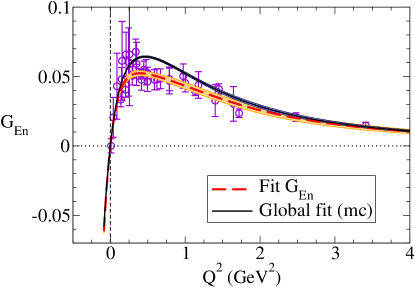
Figure 2: Neutron electric form factor. Results of the direct fit to the $G_{En}$ data (dashed line, thick band), and of the global fit without the valence quark contributions (thin band). The label “mc” stands for meson cloud. Data from Gentile11 ; Schiavilla01 .

       

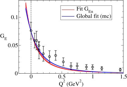
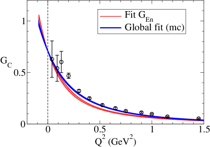
Figure 3: $\gamma^{\ast}N\to\Delta(1232)$ electric and Coulomb quadrupole form factors. Results of models with no valence quark contributions. Results of the direct fit to the $G_{En}$ data (red band), and the global fit (blue band). The label “mc” stands for meson cloud. Data for proton targets from Blomberg16a ; Stave08 ; PDG ; MIT_data ; Jlab_data1 ; Jlab_data2 .

4.2 Parametrization for $G_{En}$

In the calculation of the pion cloud contributions to $G_{E}$ and $G_{C}$, we use the parametrization of $G_{En}$ given by eq. (6), where we take $k=3$ (3 parameters). Compared to the Galster parametrization (5), we consider one additional parameter. Using eq. (6), we avoid an explicit dependence on the dipole factor $G_{D}$. This procedure may be more appropriated for the study of the $\gamma^{\ast}N\to\Delta(1232)$ transition form factors, since it avoids the connection with a scale associated exclusively with the nucleon Siegert-ND .

Fits based on parametrizations with larger values of $k$ ($k\geq 4$) lead to similar results at low $Q^{2}$, but increase the number of parameters. In addition, for $k\geq 5$, the higher order coefficients $c_{l}$ of the parametrizations are constrained mainly by the $Q^{2}>2$ GeV² data, which is restricted to 2 data points (2.48 GeV² and 3.41 GeV²). Those coefficients are therefore poorly constrained, and can lead to strong oscillations in the function $G_{En}$ for large $Q^{2}$, in conflict with the smooth falloff expected for large $Q^{2}$. Parametrizations of $G_{En}$ with $k\geq 5$ may be considered, once more information relative the function $G_{En}$ become available, such as, more and better distributed data at large $Q^{2}$.

Table 1: Parameters $c_{i}$ associated with the parametrization from eq. (6) for the case $k=3$. The brackets represent the uncertainty associated with the parameters. In the first row $\rho_{c_{i}c_{j}}$ represents the coefficient of correlation between $c_{i}$ and $c_{j}$. In the second row $\sigma_{c_{i}c_{j}}$ represent the covariance between $c_{i}$ and $c_{j}$.

	$c_{1}$ (GeV-2)	$c_{2}$ (GeV-2)	$c_{3}$ (GeV-4)	$\rho_{c_{1}c_{2}}$	$\rho_{c_{1}c_{3}}$	$\rho_{c_{2}c_{3}}$
				$\sigma_{c_{1}c_{2}}$ (GeV-4)	$\sigma_{c_{1}c_{3}}$ (GeV-6)	$\sigma_{c_{2}c_{3}}$ (GeV-6)
Fit $G_{En}$	3.39	$-0.750$	2.01	0.39	0.97	0.21
	(0.39)	(0.135)	(0.77)	(0.021)	(0.29)	(0.025)
Global fit	3.31	$-0.175$	1.71	0.84	0.97	0.69
(only meson cloud)	(0.19)	(0.113)	(0.34)	(0.019)	(0.063)	(0.026)
Global fit	3.28	$-0.954$	1.93	0.62	0.95	0.36
(total)	(0.17)	(0.077)	(0.26)	(0.0079)	(0.042)	(0.0073)
Fit $G_{En}$, $G_{E}$	3.47	$-0.744$	2.19	0.35	0.98	0.19
	(0.42)	(0.138)	(0.90)	(0.020)	(0.37)	(0.015)

4.3 Model with no valence quark contributions

In order to test whether the inclusion of the valence quark effects on the $\gamma^{\ast}N\to\Delta(1232)$ quadrupole form factors is really relevant for the description of the data, we consider first two fits where we ignore those effects.

We start with a direct fit to the $G_{En}$ data, ignoring the impact of the quadrupole form factor data. The parameters associated with the fit and the respective errors are presented in the first row of table 1. The coefficients of correlation between the parameters are also presented in the table and are discussed later. The reduced chi-square associated with the $G_{En}$ fit is 0.66, pronouncing the good quality of fit. The parameters of the global fit to the $G_{En}$, $G_{E}$ and $C_{C}$ data, using only the meson cloud term, and the corresponding errors are presented in the second row of table 1. The values of reduced chi-square associated with the different subsets and the combined chi-square per degree of freedom are presented in the second row of table 2.

From the chi-square values presented in the second row of table 2, one can anticipate that a fit that does not include additional contributions to the pion cloud parametri-zation lead to a very poor description of the $G_{C}$ data (reduced chi-square 6.7), as well as an imprecise description of the neutron electric form factor data (reduced chi-square 2.7) and the electric quadrupole form factor data (reduced chi-square 2.0).

The results of the two fits to the $G_{En}$, including the interval of variation associated with the uncertainties in the parameters are presented in fig. 2. The dashed line represent the result of the fit to the $G_{En}$ data and the uncertainties are represented by the thick band (orange). The thin band represents the result of the global fit (including the uncertainties). The range of the variation of $G_{En}$ is estimated using the propagation of errors associated with the coefficients $c_{i}$ according to the parametrization (6) with $k=3$ Errors-Taylor .

In fig. 2, we also present the results below $Q^{2}=0$ down to $Q^{2}=-(M_{\Delta}-M)^{2}\simeq-0.09$ GeV², which correspond to the pseudothreshold of the $\gamma^{\ast}N\to\Delta(1232)$ transition. As mentioned, the region below $Q^{2}=0$ is important for the study of the quadrupole form factors and to Siegert’s theorem Siegert-ND ; Letter .

The results for the quadrupole form factors, $G_{E}$ and $G_{C}$, are presented in fig. 3. In this case, the interval of variation is small (narrower bands).

The errors associated with the coefficients $c_{j}$ are determined based on standard relations that take into account the errors associated with the data and the sensibility of the parameters relative to the data. The last effect is estimated by $\left(\frac{\partial c_{j}}{\partial y_{i}}\right)$ where $y_{i}$ represent the $G_{En}$, $G_{E}$ or $G_{C}$ data Errors-Taylor ; NumericalRecipes . The available data suggest that the coefficients $c_{1}$, $c_{2}$ and $c_{3}$ are not really uncorrelated, since the coefficients of correlation between the parameters differ significantly from zero Errors-Taylor ; NumericalRecipes . The coefficients of correlation and the covariance functions are presented in the last three columns of table 1. Note in particular that the coefficient of correlation between $c_{1}$ and $c_{3}$, $\rho_{c_{1}c_{3}}$, is very close to one, indicating a strong correlation between the effect of those two coefficients. A consequence of the correlation between coefficients is that to estimate the range of variation of $G_{En}$ we cannot consider just the quadratic terms $\left(\frac{\partial G_{En}}{\partial c_{i}}\right)^{2}\sigma_{c_{i}}^{2}$ associated with $c_{1}$, $c_{2}$ and $c_{3}$, but that it is also necessary to consider the cross terms: $2\left(\frac{\partial G_{En}}{\partial c_{i}}\right)\left(\frac{\partial G_{En}}{\partial c_{j}}\right)\sigma_{c_{i}c_{j}}$, where $\sigma_{c_{i}c_{j}}$ is the covariance function between $c_{i}$ and $c_{j}$ Errors-Taylor . The narrow bands presented in the following figures are the consequence of the inclusion of the cross terms.

Table 2: Quality of the parametrizations measured in terms of chi-square per degree of freedom ($G_{En}$, $G_{E}$ and $G_{C}$). $\chi^{2}({\rm tot})$ is the total chi-square per degree of freedom. The results between brackets indicate the values associated with the sets not included in the fits.

	$\chi^{2}(G_{En})$	$\chi^{2}(G_{E})$	$\chi^{2}(G_{C})$	$\chi^{2}({\rm tot})$
Fit $G_{En}$	0.66	(2.70)	(26.5)
Global fit (mc)	2.65	2.03	6.73	2.94
Global fit	0.77	0.67	1.15	0.77
Fit $G_{En}$, $G_{E}$	0.66	0.63	(2.33)

One can now comment on the results of the fits. In fig. 2, we can notice that the direct fit to the data provide a much better description of the $G_{En}$ data (reduced chi-square 0.66) than the global fit restricted to the meson cloud term (reduced chi-square 2.65). In the last case the fit overestimates the $G_{En}$ data for $Q^{2}>0.25$ GeV². It is worth noticing that, although the combined fit reduces the errors associated with the parameters, and consequently the width of the bands associated with $G_{En}$, that does not imply that the data description is more accurate, as can be inferred from the reduced chi-square values.

As for the quadrupole form factors displayed in fig. 3, we can conclude that the combined fit (at blue) improves the description of the quadrupole form factor data compared to a fit that excludes those data (at red). The improvement is more significant for $G_{C}$. Both fits show a reasonable agreement with the data near $Q^{2}=0$. Focusing on the global fit, it is important to mention that the results are the consequence of the overestimated results for $G_{En}$, which enhance the values of $G_{E}$ and $G_{C}$ at low $Q^{2}$ in about 30%. We can also note that $G_{E}$ is poorly described for $Q^{2}>0.4$ GeV² and that the global fit of $G_{C}$ underestimates the data in the region $Q^{2}\approx 0.2$ GeV².

To summarize this first analysis, one can say that a global fit which neglects the valence quark contributions appears to give a reasonable description of the quadrupole form factor data at low $Q^{2}$. Those results, however, are a consequence of a rough description of the $G_{En}$ data.

4.4 Global fit (including the valence quark contributions)

We consider now a global fit to the data that take into account the contribution of the valence quarks on the quadrupole form factors $G_{E}$ and $G_{C}$. The inclusion of the valence quark term introduces additional uncertainties in the calculations, since there are now uncertainties associated with the quark model estimates of the functions $G_{a}^{\rm B}$ ($a=E,C$).

The simplest way of taking into account those uncertainties in the fit it is to modify the experimental standard deviation $\sigma_{i}$ associated with $G_{a}$ according to $\sigma_{i}^{2}\to\sigma_{i}^{2}+\sigma^{2}(G_{a}^{\rm B})$, in the chi-square calculation, where $\sigma(G_{a}^{\rm B})$ is the theoretical error associated with the result for $G_{a}^{\rm B}$. The previous modification is justified in the calculation of the factor $G_{a}-(G_{a}^{\rm B}+G_{a}^{\pi})$, when the errors are combined in quadrature. The main consequence of the previous procedure is the reduction of the impact of the $G_{E}$ and $G_{C}$ data in the global fit, since the contribution of each term is weighted by the factor $1/\sigma_{i}^{2}$. In those conditions the chi-square associated with the experimental data differ from the effective chi-square obtained when we include the quark model uncertainties (the model uncertainties reduce the chi-square values). The interpretation of the reduced chi-square values become less clear, then, since it is not restricted exclusively to the experimental data.

For the reasons mentioned above, we choose not to take into account explicitly the uncertainties associated with the quark model in the global fit to the data. Alternatively, we determined the chi-square taking into account the experimental errors and include the quark model uncertainties afterward in the representation of the results for $G_{E}$ and $G_{C}$. With this procedure, we preserve the usual interpretation of reduced chi-square based on the experimental data. The quark model uncertainties are taken into account later in the discussion of the results for the quadrupole form factors.

The parameters associated with the best fit to the $G_{En}$, $G_{E}$ and $G_{C}$ data, including the valence quark and meson cloud contributions on the quadrupole form factors are presented in the third row of table 1. The results for the reduced chi-square associated with the different sets of data are presented in the third row of table 2.

The chi-square values obtained in the global fit seems to suggest that all the data subsets ($G_{En}$, $G_{E}$ and $G_{C}$) are well described, since the reduced chi-square is smaller than the unit, or just a bit larger, in the case of $G_{C}$. One can then conclude that if the theoretical uncertainties are small, the inclusion of the valence quark contributions improves the global description of the data.

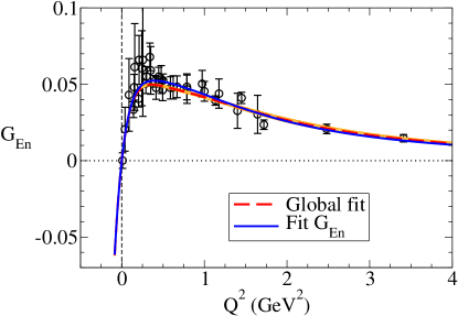
Figure 4: Neutron electric form factor. Best fit to the data (band and dashed line) compared with the direct fit and with the $G_{En}$ data (solid line). Data from Gentile11 ; Schiavilla01 .

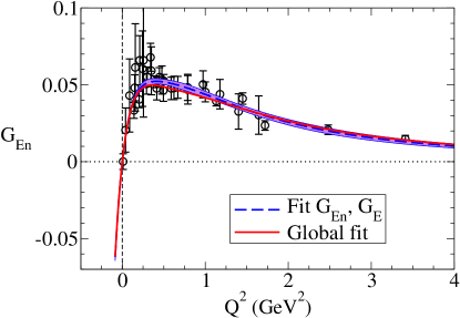
Figure 5: Neutron electric form factor. Best fit to the data (solid line) compared with the best fit to the $G_{En}$ and $G_{E}$ data (excluding the $G_{C}$ data). The bands represent the errors associated with the partial fit ($G_{En}$ and $G_{E}$). The errors associated with the global fit are not included for clarity (see fig. 2). Data from Gentile11 ; Schiavilla01 .

The numerical results for $G_{En}$ and for the quadrupole form factors $G_{E}$ and $G_{C}$ are discussed in the following subsections, including the uncertainties associated with the quark model from LatticeD . The relative uncertainties associated with the quark model can be determined numerically combining the lattice QCD results $G_{a}^{\rm latt}$ with the model estimate of that result in lattice $G_{a}^{\rm B}$. One conclude then that the errors associated with the functions $G_{E}^{\rm B}$ and $G_{C}^{\rm B}$ can be expressed as $\sigma(G_{E}^{\rm B})=0.45\,G_{E}^{\rm B}$ and $\sigma(G_{C}^{\rm B})=0.33\,G_{C}^{\rm B}$. The comparison of the results of the quark model with lattice QCD results is possible because the meson cloud effects are suppressed in lattice QCD simulations with large pion masses LatticeD . The lattice QCD results for $G_{E}$ and $G_{C}$ are calculated from the results for $G_{E}/G_{M}$ and $G_{C}/G_{M}$, which have uncertainties much larger than $G_{M}$. In total one has 21 points for $G_{E}$ and 21 points for $G_{C}$ for $m_{\pi}=411$, 490 and 593 MeV LatticeD ; Alexandrou08 .

4.5 Neutron electric form factor ($G_{En}$)

We now discuss the numerical results for $G_{En}$ presented in fig. 4 (solid line) in comparison with the data from Gentile11 ; Schiavilla01 .

The quality of the description of the $G_{En}$ data and the narrow band of variation can be observed in detail in fig. 4, where we include also the results of the single fit to the $G_{En}$ data, where we neglect the effect if the $G_{E}$ and $G_{C}$ data. In the last case, we omit the band of variation associated with the first model (fit $G_{En}$) for clarity. The comparison with the results from fig. 2 is sufficient to show that the errors associated with the function $G_{En}$ are reduced when we consider the global fit. Based on the results presented in the third row of table 1, one can conclude that the errors associated the parameters decrease compared to the previous fits, justifying the thin band of variation presented in the figure.

       

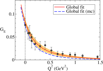
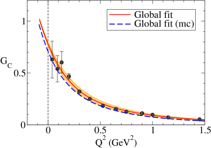
Figure 6: $\gamma^{\ast}N\to\Delta(1232)$ electric and Coulomb quadrupole form factors. Best global fit to the data (solid line, orange band). The result of the best fit without valence quark contributions is also presented (dashed line, “mc” stands for meson cloud) for comparison. Data for proton targets from Blomberg16a ; Stave08 ; PDG ; MIT_data ; Jlab_data1 ; Jlab_data2 .

The parametrization presented in fig. 4 correspond to the value

$$r_{n}^{4}=(-0.383\pm 0.012)\;\mbox{fm}^{4}.$$ (8)

This estimate is close to other estimates presented in the literature based on the Galster parametrization Grabmayr01 and similar parametrizations Kaskulov04 . For the purpose of the discussion, we note that a Galster parametrization that provides a good description of the $G_{En}$ data, associated with $d=2.8$ correspond to $r_{n}^{4}\simeq-0.30$ fm⁴ Siegert-ND ; Letter ; Buchmann04 .

It is also worth mentioning that in a parametrization that include the factor $G_{D}$, a significant contribution to $r_{n}^{4}$ comes from a term on $1/\Lambda^{2}$, where $\Lambda^{2}=0.71$ GeV². When we consider a Galster parametrization, the last contribution is about $-0.25$ fm⁴. It is then interesting to conclude that we obtain a result close to the Galster parametrizations, without including the factor $G_{D}$.

The comparison between the results for the third moment is even more compelling. We obtain almost the same result for $r_{n}^{6}$: $r_{n}^{6}=(-1.31\pm 0.12)$ fm⁶, using the parametri-zation with rational functions and $r_{n}^{6}\simeq-1.34$ fm⁶, using the Galster parametrization with $d=2.8$ Siegert-ND ; Letter ; Buchmann04 . We conclude then that the two paramerizations are distinguished near $Q^{2}=0$, within the uncertainties, basically by the value of the second moment ($r_{n}^{4}$).

In figs. 2 and 4, we can notice that the different parame-trizations have a very similar extension to the timelike region, including the pseudothreshold. Very similar results can also be obtained with the Galster parametrization. This effect is explained by the dominance of the first two terms (first and second moments) in the expansion of $G_{En}$ from (4) near the pseudothreshold.

In order to test the dependence of the fit on the data subsets, we perform also partial fits to the combination of the data $(G_{En},G_{E})$ and $(G_{En},G_{C})$. This way, we test which quadrupole set, $G_{E}$ or $G_{C}$, has more impact in the global fit, and we can also infer if those sets are compatible with the $G_{En}$ data. The result of the fit to the sets $(G_{En},G_{C})$ is represented in fig. 5 by the blue band. The global fit ($G_{En}$, $G_{E}$ and $G_{C}$) is represented by the solid line. The result of the combined fit for $(G_{En},G_{C})$ is almost undistinguished from the global fit (solid line), and it is not presented for clarity. The parameters associated with the partial fit $(G_{En},G_{E})$ are presented in the last row of table 1. Compared to the global fit, we notice the increasing errors associated with the parameters. The corresponding values for the reduced chi-square are presented in the last row of table 2. From the result for $\chi^{2}(G_{C})$ we can confirm that the quality of the description of the $G_{En}$ and $G_{E}$ is obtained at the expenses of a poorer description of the $G_{C}$ data.

In the literature, there is some debate whether there is a bump in the function $G_{En}$ near $Q^{2}=0.2$–0.3 GeV², or not Pascalutsa07a ; Friedrich03 . We conclude that the present accuracy of the data is insufficient for more definitive conclusions. Our best fit has a smooth behavior in the region under discussion. Nevertheless, larger values of $k$ can in principle generate a low-$Q^{2}$ bump, once one has more high $Q^{2}$ data to constrain the higher order coefficients.

When we take into account the theoretical uncertainties associated with the quark model the results for $G_{En}$ are only somewhat modified. The magnitude of $G_{En}$ is slightly enhanced near $Q^{2}=0.5$ GeV².

4.6 Quadrupole form factors ($G_{E}$, $G_{C}$)

The results of the best global fit to the $\gamma^{\ast}N\to\Delta(1232)$ quadrupole form factors (solid line) including the theoretical uncertainties (orange band) are presented in fig. 6, in comparison with the respective data. For comparison, we include also the previous fit where we ignore the valence quark contributions (dashed line).

Focusing first in the central values (solid line) we observe an excellent agreement with the data in the range $Q^{2}=0$–1.5 GeV², for both form factors. As mentioned before, the quality of the description is corroborated by the reduced chi-square values presented in table 2, 0.67 and 1.15 for $G_{E}$ and $G_{C}$, respectively. For this agreement contributes the larger error bars for the data below 0.2 GeV². The precision of the $Q^{2}<0.2$ GeV² data is comparable to the precision of most of the neutron electric form factor data. We note, however, that in the present case it is not sufficient to look for the chi-square values, because there are also uncertainties associated with the valence quark contributions.

The uncertainties displayed in fig. 6 are the combination of the pion cloud uncertainties associated with the $G_{En}$ parametrization and the uncertainties associated with the quark model. The main contribution comes from the quark model. The magnitude of the pion cloud uncertainties can be inferred from fig. 3. The uncertainties are very small at pseudothreshold because according to our estimate, the uncertainties associated with the valence quark contribution vanish and only the pion cloud component contributes (recall that $G_{E}^{\rm B}$ and $G_{C}^{\rm B}$ vanish at pseudothreshold).

The results from fig. 6 shows that there is a range of variation of $G_{E}^{\rm B}$ and $G_{C}^{\rm B}$ which give a better solution than models with no valence quark contributions. In the figure, we can notice that the model with no valence quark contributions (dashed line) is a bit below the lower limit of the estimate with valence quark contributions. One can then conclude that the inclusion of the bare contribution improves the description of the data.

The lower limit of the results for $G_{E}$ is obtained for a bare contribution of about $0.55\,G_{E}^{B}$, where $G_{E}^{B}$ is the estimate of the covariant spectator quark model. In this case, we cannot conclude much, since theoretical and experimental uncertainties are both large and compatible.

The improvement is more significant in the case of $G_{C}$ with a much narrower band of variation. In this case, the model uncertainties are about 33% of the model estimate $G_{C}^{B}$. One can notice in this case, that although the fit with no valence quark component (dashed line) is just a bit below the lower limit of the model estimate, the reduced chi-square values are very different (see table 2). The difference between those values is a consequence of the small error bars associated with the $Q^{2}>0.2$ GeV² data for $G_{C}$. One concludes, then that $G_{C}$ is more sensitive to the inclusion of the valence quark component.

The comparison of results of $G_{E}$ with $G_{C}$ corrected by the factor $\kappa$ is presented in fig. 7. For clarity, we omit the uncertainties associated with both form factors. In this representation, it is more explicit the connection between the two quadrupole form factors and the implications of Siegert’s theorem. The convergence of the results at the pseudothreshold ($Q^{2}\simeq-0.09$ GeV²), the consequence of Siegert’s theorem, is clearly displayed in the graph.

In comparison with the results from Letter , where $G_{En}$ is described by a Galster parametrization ($d=2.8$), we obtain slightly larger values for the quadrupole form factors at the pseudothreshold.

Based on the results of $G_{E}$ and $G_{C}$ at $Q^{2}=0$, one can test the accuracy of the large $N_{c}$ estimate $G_{E}={\textstyle\frac{M_{\Delta}^{2}-M^{2}}{4M_{\Delta}^{2}}}G_{C}$, apart ${\cal O}({\textstyle\frac{1}{N_{c}^{2}}})$ relative corrections Pascalutsa07a . The previous relation is equivalent to the identity $R_{EM}(0)=R_{SM}(0)$ Letter ; Pascalutsa07a . According to the results from figs. 6 and 7, one obtains $G_{E}(0)=0.083\pm 0.003$ and ${\textstyle\frac{M_{\Delta}^{2}-M^{2}}{4M_{\Delta}^{2}}}G_{C}(0)=0.082\pm 0.004$, in agreement with the large $N_{c}$ prediction, within the uncertainties.

4.7 Square radii $r_{E}^{2}$ and $r_{C}^{2}$

The difference of behavior between the two quadrupole form factors can be better understood when we look at the square radius associated with the quadrupole form factors $G_{E}$ and $G_{C}$, defined by Buchmann09a ; SiegertD ; Forest66

$$r_{a}^{2}=-\frac{14}{G_{a}(0)}\left.\frac{dG_{a}}{dQ^{2}}\right|_{Q^{2}=0}$$ (9)

where $a=E,C$. The numerical results for $r_{E}^{2}$ and $r_{C}^{2}$ for the parametrizations discussed here are presented in table 3.

If we ignore the effect of the valence quarks, one can calculate $r_{E}^{2}$ and $r_{C}^{2}$ very easily using eq. (2)-(3). One obtains then $r_{E}^{2}=\frac{7}{10}\frac{r_{n}^{4}}{r_{n}^{2}}+{\textstyle\frac{7}{M_{\Delta}(M_{\Delta}-M)}}$ and $r_{C}^{2}=\frac{7}{10}\frac{r_{n}^{4}}{r_{n}^{2}}$. We conclude then that $r_{E}^{2}-r_{C}^{2}$ is of order $N_{c}^{0}$, and it is not suppressed in the large $N_{c}$ limit. The relation for $r_{C}^{2}$ was derived previously in Buchmann09a , assuming the dominance of the pion cloud contribution. Using the result (8) for $r_{n}^{4}$, one obtains the estimates $r_{E}^{2}=3.06\pm 0.07$ fm² and $r_{C}^{2}=2.31\pm 0.07$ fm². The uncertainties in the previous results are the consequence of the results for $r_{n}^{4}$, affected by the errors associated with the parametrization $G_{En}$. Both estimates are about 10% larger than the results for the pion cloud contribution presented in table 3, and are therefore consistent with a 10% correction for both form factors near $Q^{2}=0$, due to the inclusion of the valence quark contributions, as discussed in sect. 2.

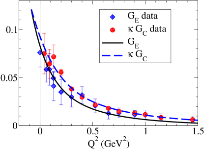
Figure 7: Results for the form factors $G_{E}$ and $G_{C}$. Recall that $\kappa={\textstyle\frac{M_{\Delta}-M}{2M_{\Delta}}}\simeq 0.12$. Data for proton targets from Blomberg16a ; Stave08 ; PDG ; MIT_data ; Jlab_data1 ; Jlab_data2 .

Combining the analytic expressions described previously for $r_{E}^{2}$ and $r_{C}^{2}$, one has $r_{E}^{2}-r_{C}^{2}={\textstyle\frac{7}{M_{\Delta}(M_{\Delta}-M)}}\simeq 0.75$ fm². Note that this result is independent of the general form used for the function $G_{En}$, and therefore independent of $r_{n}^{4}$.

The previous estimate differs from the result presented in table 3, mostly because of the valence quark effects are not taken into account as discussed above (10% reduction). Correcting the previous result with the valence quark effect, assuming the 10% correction, one obtains then $(r_{E}^{2}-r_{C}^{2})_{\pi}\simeq 0.68$ fm². The subindex was included to emphasize that the estimate concerns the pion cloud component. The previous estimate is still in disagreement with the result from table 3, in about $-0.04$ fm². In this discussion, we omit the uncertainties and focus on the results obtained with the central values presented in the table.

To understand the small difference of $-0.04$ fm², we need to look into the details of the calculation, and for the very small deviations from the 10% correction, assumed for the valence quark component. If we consider deviation of $\delta_{E}$ and $\delta_{C}$ from the 10% correction to the form factors $G_{E}$ and $G_{C}$, respectively, we conclude that the residual correction can be expressed as $0.9^{2}(\delta_{C}-\delta_{E})r_{E0}^{2}$, where the first factor accounts for the 10% correction in the normalizations, and $r_{E0}^{2}$ is the estimate of $r_{E}^{2}$ in a model with pion cloud dominance, mentioned above. Combining all effects with $r_{E0}^{2}\simeq 3.06$ fm², one obtain $0.9^{2}(\delta_{C}-\delta_{E})r_{E0}^{2}\simeq-0.04$ fm², which explain at last the result $(r_{E}^{2}-r_{C}^{2})_{\pi}\simeq 0.64$ fm². The last correction is then the consequence of the product of a very small factor by a large factor ($r_{E0}^{2}$).

The contributions from the valence quark component depend on the details of the quark model, and are therefore model dependent. Using the model described previously, we obtain $(r_{E}^{2}-r_{C}^{2})_{\rm B}\simeq-0.06$ fm², where B labels the bare contribution. Combining the two contributions, we obtain $r_{E}^{2}-r_{C}^{2}\simeq 0.58$ fm², as presented in table 3. When we take into account all the errors we obtain $r_{E}^{2}-r_{C}^{2}=0.58\pm 0.23$ fm² (see table 3).

Table 3: Contributions to the quadrupole square radius (bare and pion cloud): $r_{E}^{2}$, $r_{C}^{2}$ and difference $r_{E}^{2}-r_{C}^{2}$. The results between brackets indicate the uncertainties.

	$r_{E}^{2}$ (fm2)	$r_{C}^{2}$ (fm2)	$r_{E}^{2}-r_{C}^{2}$ (fm2)
B	$-0.410$	$-0.347$	$-0.063$
	$\;\;\;(0.169)$	$\;\;\;(0.107)$	$\;\;\;(0.200)$
$\pi$	$\;\;\;2.742$	$\;\;\;2.100$	$\;\;\;0.643$
	$\;\;\;(0.080)$	$\;\;\;(0.064)$	$\;\;\;(0.102)$
Total	$\;\;\;2.331$	$\;\;\;1.752$	$\;\;\;0.580$
	$\;\;\;(0.187)$	$\;\;\;(0.134)$	$\;\;\;(0.225)$

Smaller values for $r_{C}^{2}$ have been suggested by empirical parametrizations of the quadrupole form factor data consistent with Siegert’s theorem Siegert-ND ; SiegertD . We note, however, that those estimates are strongly affected by the $Q^{2}=0$–0.15 GeV² data for $G_{C}$, from Stave08 ; MIT_data ; Sparveris13 . Therefore, the conclusions based on those data have to be reviewed in light of the new data from Blomberg16a .

An important conclusion of the previous discussion is that in order to obtain a reliable estimate of $r_{E}^{2}$ and $r_{C}^{2}$ from the $G_{E}$ and $G_{C}$ data, we need more accurate measurements from $G_{E}$ and $G_{C}$ near $Q^{2}=0$.

Overall, we can conclude that the large values obtained for $r_{E}^{2}$ and $r_{C}^{2}$ are the outcome of the pion cloud dominance. The magnitudes of $r_{E}^{2}$ and $r_{C}^{2}$ around 2 fm² can be interpreted physically, as the result of the increment of the size of the constituent quarks due to the $q\bar{q}$ pair/pion cloud dressing Buchmann09a ; SiegertD . More specifically, those magnitudes can be understood looking at the pion Compton scattering wavelength, $r_{\pi}\approx 1/m_{\pi}$, which characterize the pion distribution inside the nucleon Buchmann09a . Numerically, the result $r_{E}^{2}\approx r_{C}^{2}\approx 2$ fm² is then the consequence of $r_{E}^{2}\approx r_{C}^{2}\approx r_{\pi}^{2}$. A more detailed discussion on this subject can be found in Buchmann09a .

Concerning the difference $r_{E}^{2}-r_{C}^{2}=0.6\pm 0.2$ fm², one can conclude that it is mainly a consequence of Siegert’s theorem, since the difference between $r_{E}^{2}$ and $r_{C}^{2}$ is the consequence of the extra factor included in the pion cloud parametrization $G_{E}^{\pi}$, in order to satisfy Siegert’s theorem.

4.8 General discussion

Once presented our final results for the neutron electric form factor and for $\gamma^{\ast}N\to\Delta(1232)$ quadrupole form factors, one can discuss some theoretical and experimental aspects related to the present results.

For the good agreement between the model and the data for the quadrupole form factors, displayed in figs. 6 and 7 contributes the valence quark component estimated with a covariant quark model. We stress that this part of the calculation is model dependent and it is then limited by some theoretical uncertainties. Those uncertainties are larger in the case of the electric form factor $G_{E}$. Alternative estimates of the valence quark contribution, with the same sign, can also improve the description of the quadrupole form factor data. An example is the bare para-metrization of the Sato-Lee model in the $Q^{2}>0$ region LatticeD ; SatoLee . Another example is the estimates based on the Dyson-Schwinger formalism, which are expected to be closer to the upper limit of the present calculation.

A test to the valence quark contributions can be performed in a near future with lattice QCD simulations in the range of $m_{\pi}=0.2$–0.3 GeV Alexandrou11 , a region close the physical point, but where hopefully the pion cloud contamination is small. The increase of the number of lattice QCD simulations and of the accuracy of those simulations can also help to improve the accuracy of the present quark model estimates.

Another relevant point of discussion is the accuracy of the data. The data associated with $G_{En}$ have in general large error bars, which difficult the derivation of an accurate parametrization. The $G_{E}$ and $G_{C}$ data below 0.15 GeV² are also affected by large error bars. In that region the experimental uncertainties are larger than the quark model uncertainties. For all those reasons it is not hard to find parametrizations that provides a good description of the overall data, including the low-$Q^{2}$ region (small chi-square). The inclusion of the $G_{E}$ and $G_{C}$ data provide, however, additional constraints to the function $G_{En}$, which help to pin down the shape of $G_{En}$.

Another important aspect of the present work is the sensitivity of the fits to the data, particularly in the region $Q^{2}=0$–0.2 GeV². This effect can be illustrated by the realization that the trend of the function $G_{C}$ changed with the more recent data Blomberg16a . A fit that includes the $G_{C}$ data from Stave08 ; MIT_data cannot describe the data with the same accuracy as a fit that include the more recent data Siegert-ND . In conclusion, new data for $G_{C}$ have also a significant impact on the solution for $G_{En}$.

To finish the present discussion, we note that we can also test the results of the functions $G_{E}$ and $G_{C}$ combining lattice QCD results with estimates based on expansions on the pion mass, derived from effective field theories Pascalutsa05 ; Gail06 ; Hilt18 . In these conditions the consistency between the results from lattice QCD and the experimental data can be checked, and therefore, the consistency between QCD and the real world.

5 Outlook and conclusions

In the present work, we derive a global parametrization of the neutron electric form factor and the $\gamma^{\ast}N\to\Delta(1232)$ quadrupole form factors, $G_{E}$ and $G_{C}$. To relate the pion cloud contribution to $G_{E}$ and $G_{C}$ with the neutron electric form factor we use improved relations derived in the large $N_{c}$ limit in order to verify Siegert’s theorem exactly.

The success of the global parametrization of $G_{En}$, $G_{E}$ and $G_{C}$ is an indication of the importance of the pion cloud in the neutron and in the $\gamma^{\ast}N\to\Delta(1232)$ transition. This correlation is suggested by the large $N_{c}$ limit, by the $SU(6)$ symmetry breaking, and by calculations based on non relativistic constituent quark models.

For the agreement between the model calculations and the empirical data for the $\gamma^{\ast}N\to\Delta(1232)$ quadrupole form factors also contribute the small valence quark components estimated by a covariant quark model, calibrated previously by the results of lattice QCD simulations. Although limited by some model uncertainties, the estimates of the valence quark contributions improve the description of the data compared to models with no bare contributions. Estimates of the valence quark effects based on other frameworks may also improve the description of the $\gamma^{\ast}N\to\Delta(1232)$ quadrupole form factors.

The global fit of the $G_{En}$, $G_{E}$ and $G_{C}$ data, based on rational functions, show that the overall data, and the $G_{En}$ data, in particular, is compatible with a smooth description of the neutron electric form factor with no pronounced bump at low $Q^{2}$. The best description of the data is obtained when we consider a parametrization of $G_{En}$ associated with $r_{n}^{4}=-0.38\pm 0.01$ fm⁴.

We conclude that the square radii associated with the quadrupole form factors $G_{E}$ and $G_{C}$ are large, as a consequence of the pion cloud effects (long extension of the pion cloud). We also conclude that the square radii, $r_{E}^{2}$ and $r_{C}^{2}$ are constrained by the relation $r_{E}^{2}-r_{C}^{2}=0.6\pm 0.2$ fm². The previous relation is a consequence of Siegert’s theorem and of the dominance of the pion cloud contributions on the quadrupole form factors $G_{E}$ and $G_{C}$.

The present parametrization of the neutron electric form factor is still derived from data with significant error bars below 0.2 GeV². Future experiments with more accurate data for $G_{En}$, and the $\gamma^{\ast}N\to\Delta(1232)$ quadrupole form factors can help to elucidate the shape of the function $G_{En}$ at low $Q^{2}$. Of particular interest are the upcoming results of the JLab 12-GeV upgrade NSTAR ; NSTAR2017 .

References

- (1) I. G. Aznauryan et al., Int. J. Mod. Phys. E 22, 1330015 (2013) [arXiv:1212.4891 [nucl-th]].
- (2) V. Pascalutsa, M. Vanderhaeghen and S. N. Yang, Phys. Rept. 437, 125 (2007) [hep-ph/0609004].
- (3) I. G. Aznauryan and V. D. Burkert, Prog. Part. Nucl. Phys. 67, 1 (2012) [arXiv:1109.1720 [hep-ph]].
- (4) H. F. Jones and M. D. Scadron, Annals Phys. 81, 1 (1973).
- (5) M. A. B. Beg, B. W. Lee and A. Pais, Phys. Rev. Lett. 13, 514 (1964).
- (6) C. Becchi and G. Morpurgo, Phys. Lett. 17, 352 (1965).
- (7) B. Julia-Diaz, T.-S. H. Lee, T. Sato and L. C. Smith, Phys. Rev. C 75, 015205 (2007) [nucl-th/0611033].
- (8) G. Ramalho, M. T. Peña and F. Gross, Eur. Phys. J. A 36, 329 (2008) [arXiv:0803.3034 [hep-ph]].
- (9) G. Ramalho and M. T. Peña, J. Phys. G 36, 115011 (2009) [arXiv:0812.0187 [hep-ph]].
- (10) G. Ramalho and K. Tsushima, Phys. Rev. D 87, 093011 (2013) [arXiv:1302.6889 [hep-ph]].
- (11) G. Ramalho and K. Tsushima, Phys. Rev. D 88, 053002 (2013) [arXiv:1307.6840 [hep-ph]].
- (12) G. Eichmann and D. Nicmorus, Phys. Rev. D 85, 093004 (2012) [arXiv:1112.2232 [hep-ph]].
- (13) J. Segovia, C. Chen, C. D. Roberts and S. Wan, Phys. Rev. C 88, 032201 (2013) [arXiv:1305.0292 [nucl-th]].
- (14) H. Sanchis-Alepuz, R. Alkofer and C. S. Fischer, Eur. Phys. J. A 54, 41 (2018) [arXiv:1707.08463 [hep-ph]].
- (15) N. Isgur, G. Karl and R. Koniuk, Phys. Rev. D 25, 2394 (1982).
- (16) S. Capstick and G. Karl, Phys. Rev. D 41, 2767 (1990).
- (17) G. Ramalho, M. T. Peña and F. Gross, Phys. Rev. D 78, 114017 (2008) [arXiv:0810.4126 [hep-ph]].
- (18) G. Ramalho and M. T. Peña, Phys. Rev. D 80, 013008 (2009) [arXiv:0901.4310 [hep-ph]].
- (19) G. Ramalho, Phys. Rev. D 94, 114001 (2016) [arXiv:1606.03042 [hep-ph]].
- (20) G. Ramalho, Eur. Phys. J. A 54, 75 (2018) [arXiv:1709.07412 [hep-ph]].
- (21) S. L. Glashow, Physica A 96, 27 (1979).
- (22) A. M. Bernstein, Eur. Phys. J. A 17, 349 (2003) [hep-ex/0212032].
- (23) A. J. Buchmann, E. Hernandez and A. Faessler, Phys. Rev. C 55, 448 (1997) [nucl-th/9610040].
- (24) M. I. Krivoruchenko and M. M. Giannini, Phys. Rev. D 43, 3763 (1991).
- (25) A. J. Buchmann and E. M. Henley, Phys. Rev. C 63, 015202 (2000) [arXiv:hep-ph/0101027].
- (26) G. Ramalho, M. T. Peña and A. Stadler, Phys. Rev. D 86, 093022 (2012) [arXiv:1207.4392 [nucl-th]].
- (27) G. Ramalho, M. T. Peña and F. Gross, Phys. Lett. B 678, 355 (2009) [arXiv:0902.4212 [hep-ph]].
- (28) G. Ramalho, M. T. Peña and F. Gross, Phys. Rev. D 81, 113011 (2010) [arXiv:1002.4170 [hep-ph]].
- (29) L. Tiator, D. Drechsel, S. Kamalov, M. M. Giannini, E. Santopinto and A. Vassallo, Eur. Phys. J. A 19, 55 (2004) [nucl-th/0310041].
- (30) S. S. Kamalov and S. N. Yang, Phys. Rev. Lett. 83, 4494 (1999) [nucl-th/9904072];
- (31) S. S. Kamalov, S. N. Yang, D. Drechsel, O. Hanstein and L. Tiator, Phys. Rev. C 64, 032201 (2001) [nucl-th/0006068].
- (32) T. Sato and T. S. H. Lee, Phys. Rev. C 63, 055201 (2001) [nucl-th/0010025].
- (33) V. Pascalutsa and M. Vanderhaeghen, Phys. Rev. D 76, 111501 (2007) [arXiv:0711.0147 [hep-ph]].
- (34) M. Fiolhais, B. Golli and S. Širca, Phys. Lett. B 373, 229 (1996) [hep-ph/9601379].
- (35) D. H. Lu, A. W. Thomas and A. G. Williams, Phys. Rev. C 55, 3108 (1997) [nucl-th/9612017].
- (36) G. Ramalho, Few Body Syst. 59, 92 (2018) [arXiv:1801.01476 [hep-ph]].
- (37) A. J. Buchmann, Phys. Rev. Lett. 93, 212301 (2004) [hep-ph/0412421].
- (38) P. Grabmayr and A. J. Buchmann, Phys. Rev. Lett. 86, 2237 (2001) [hep-ph/0104203].
- (39) A. J. Buchmann, Can. J. Phys. 87, 773 (2009) [arXiv:0910.4747 [physics.atom-ph]].
- (40) A. J. Buchmann, J. A. Hester and R. F. Lebed, Phys. Rev. D 66, 056002 (2002) [hep-ph/0205108].
- (41) A. Blomberg et al., Phys. Lett. B 760, 267 (2016) [arXiv:1509.00780 [nucl-ex]].
- (42) G. Ramalho, Phys. Rev. D 93, 113012 (2016) [arXiv:1602.03832 [hep-ph]].
- (43) A. J. Buchmann, E. Hernandez, U. Meyer and A. Faessler, Phys. Rev. C 58, 2478 (1998).
- (44) D. Drechsel, S. S. Kamalov and L. Tiator, Eur. Phys. J. A 34, 69 (2007) [arXiv:0710.0306 [nucl-th]].
- (45) L. Tiator and S. Kamalov, AIP Conf. Proc. 904, 191 (2007) [nucl-th/0610113].
- (46) L. Tiator, Few Body Syst. 57, 1087 (2016).
- (47) G. Ramalho, Phys. Lett. B 759, 126 (2016) [arXiv:1602.03444 [hep-ph]].
- (48) S. Galster, H. Klein, J. Moritz, K. H. Schmidt, D. Wegener and J. Bleckwenn, Nucl. Phys. B 32, 221 (1971).
- (49) J. J. Kelly, Phys. Rev. C 66, 065203 (2002) [hep-ph/0204239].
- (50) J. Friedrich and T. Walcher, Eur. Phys. J. A 17, 607 (2003) [hep-ph/0303054].
- (51) W. Bertozzi, J. Friar, J. Heisenberg and J. W. Negele, Phys. Lett. 41B, 408 (1972).
- (52) S. Platchkov et al., Nucl. Phys. A 510, 740 (1990).
- (53) M. M. Kaskulov and P. Grabmayr, Eur. Phys. J. A 19, 157 (2004) [nucl-th/0308015].
- (54) T. R. Gentile and C. B. Crawford, Phys. Rev. C 83, 055203 (2011).
- (55) N. Kaiser, Phys. Rev. C 68, 025202 (2003) [nucl-th/0302072].
- (56) M. A. Belushkin, H.-W. Hammer and U.-G. Meissner, Phys. Rev. C 75, 035202 (2007) [hep-ph/0608337].
- (57) H. W. Hammer and U. G. Meissner, Eur. Phys. J. A 20, 469 (2004) [hep-ph/0312081].
- (58) I. T. Lorenz, H.-W. Hammer and U. G. Meissner, Eur. Phys. J. A 48, 151 (2012) [arXiv:1205.6628 [hep-ph]].
- (59) G. Eichmann and G. Ramalho, Phys. Rev. D 98, 093007 (2018) [arXiv:1806.04579 [hep-ph]].
- (60) F. Gross, G. Ramalho and M. T. Peña, Phys. Rev. C 77, 015202 (2008) [nucl-th/0606029].
- (61) N. Isgur, G. Karl and D. W. L. Sprung, Phys. Rev. D 23, 163 (1981).
- (62) N. Isgur and G. Karl, Phys. Rev. D 19, 2653 (1979) Erratum: [Phys. Rev. D 23, 817 (1981)].
- (63) N. Isgur and G. Karl, Phys. Rev. D 20, 1191 (1979).
- (64) G. Dillon and G. Morpurgo, Phys. Lett. B 448, 107 (1999).
- (65) A. J. Buchmann and E. M. Henley, Phys. Rev. D 65, 073017 (2002).
- (66) A. J. Buchmann and R. F. Lebed, Phys. Rev. D 62, 096005 (2000) [hep-ph/0003167].
- (67) E. E. Jenkins, X. Ji and A. V. Manohar, Phys. Rev. Lett. 89, 242001 (2002) [hep-ph/0207092].
- (68) D. B. Lichtenberg, Unitary Symmetry and Elementary Particles, (Academic Press, New York, 1978).
- (69) F. E. Close, An Introduction to Quarks and Partons, (Academic Press, London 1979).
- (70) A. Buchmann, E. Hernandez and K. Yazaki, Phys. Lett. B 269, 35 (1991).
- (71) C. V. Christov, A. Blotz, H. C. Kim, P. Pobylitsa, T. Watabe, T. Meissner, E. Ruiz Arriola and K. Goeke, Prog. Part. Nucl. Phys. 37, 91 (1996) [hep-ph/9604441].
- (72) D. H. Lu, A. W. Thomas and A. G. Williams, Phys. Rev. C 57, 2628 (1998) [nucl-th/9706019].
- (73) L. Tiator and S. Kamalov, AIP Conf. Proc. 904, 191 (2007) [nucl-th/0610113].
- (74) L. Tiator, D. Drechsel, S. S. Kamalov and M. Vanderhaeghen, Eur. Phys. J. ST 198, 141 (2011).
- (75) D. Drechsel and M. M. Giannini, Phys. Lett. 143B, 329 (1984).
- (76) M. Weyrauch and H. J. Weber, Phys. Lett. B 171, 13 (1986) [Phys. Lett. B 181, 415 (1986)].
- (77) M. Bourdeau and N. C. Mukhopadhyay, Phys. Rev. Lett. 58, 976 (1987).
- (78) C. E. Carlson and N. C. Mukhopadhyay, Phys. Rev. Lett. 81, 2646 (1998) [hep-ph/9804356];
- (79) C. E. Carlson, Phys. Rev. D 34, 2704 (1986).
- (80) S. Stave et al. [A1 Collaboration], Phys. Rev. C 78, 025209 (2008) [arXiv:0803.2476 [hep-ex]].
- (81) C. Alexandrou, G. Koutsou, H. Neff, J. W. Negele, W. Schroers and A. Tsapalis, Phys. Rev. D 77, 085012 (2008) [arXiv:0710.4621 [hep-lat]].
- (82) G. Ramalho, K. Tsushima and F. Gross, Phys. Rev. D 80, 033004 (2009) [arXiv:0907.1060 [hep-ph]].
- (83) K. A. Olive et al. [Particle Data Group Collaboration], Chin. Phys. C 38, 090001 (2014).
- (84) R. Schiavilla and I. Sick, Phys. Rev. C 64, 041002 (2001) [arXiv:nucl-ex/0107004].
- (85) T. Eden et al., Phys. Rev. C 50, 1749 (1994).
- (86) I. Passchier et al., Phys. Rev. Lett. 82, 4988 (1999) [arXiv:nucl-ex/9907012].
- (87) C. Herberg et al., Eur. Phys. J. A 5, 131 (1999).
- (88) D. I. Glazier et al., Eur. Phys. J. A 24, 101 (2005) [arXiv:nucl-ex/0410026].
- (89) J. Bermuth et al., Phys. Lett. B 564, 199 (2003) [nucl-ex/0303015].
- (90) H. Zhu et al. [E93026 Collaboration], Phys. Rev. Lett. 87, 081801 (2001) [arXiv:nucl-ex/0105001];
- (91) R. Madey et al. [E93-038 Collaboration], Phys. Rev. Lett. 91, 122002 (2003) [arXiv:nucl-ex/0308007];
- (92) G. Warren et al. [Jefferson Lab E93-026 Collaboration], Phys. Rev. Lett. 92, 042301 (2004) [arXiv:nucl-ex/0308021].
- (93) E. Geis et al. [BLAST Collaboration], Phys. Rev. Lett. 101, 042501 (2008) [arXiv:0803.3827 [nucl-ex]].
- (94) S. Riordan et al., Phys. Rev. Lett. 105, 262302 (2010) [arXiv:1008.1738 [nucl-ex]].
- (95) V. I. Mokeev, https://userweb.jlab.org/~mokeev/resonance_electrocouplings/
- (96) N. F. Sparveris et al. [OOPS Collaboration], Phys. Rev. Lett. 94, 022003 (2005).
- (97) J. J. Kelly et al., Phys. Rev. C 75, 025201 (2007) [nucl-ex/0509004].
- (98) I. G. Aznauryan et al. [CLAS Collaboration], Phys. Rev. C 80, 055203 (2009) [arXiv:0909.2349 [nucl-ex]].
- (99) N. Sparveris et al., Eur. Phys. J. A 49, 136 (2013) [arXiv:1307.0751 [nucl-ex]].
- (100) J. R. Taylor, An introduction to the Error Analysis, ch. 9. University Science Books (1997).
- (101) W. H. Press, S. A. Teukolsky, W. T. Vetterling and B. P. Flannery, Numerical Recipes in FORTRAN: The Art of Scientific Computing, ch. 15. Press Syndicate of the University of Cambridge (1997).
- (102) T. De Forest, Jr. and J. D. Walecka, Adv. Phys. 15, 1 (1966).
- (103) C. Alexandrou, G. Koutsou, J. W. Negele, Y. Proestos and A. Tsapalis, Phys. Rev. D 83, 014501 (2011) [arXiv:1011.3233 [hep-lat]].
- (104) V. Pascalutsa and M. Vanderhaeghen, Phys. Rev. Lett. 95, 232001 (2005) [hep-ph/0508060].
- (105) T. A. Gail and T. R. Hemmert, Eur. Phys. J. A 28, 91 (2006) [nucl-th/0512082].
- (106) M. Hilt, T. Bauer, S. Scherer and L. Tiator, Phys. Rev. C 97, 035205 (2018) [arXiv:1712.08904 [nucl-th]].