Optimal designs for regression with spherical data

Abstract

In this paper optimal designs for regression problems with spherical predictors of arbitrary dimension are considered. Our work is motivated by applications in material sciences, where crystallographic textures such as the missorientation distribution or the grain boundary distribution (depending on a four dimensional spherical predictor) are represented by series of hyperspherical harmonics, which are estimated from experimental or simulated data.
For this type of estimation problems we explicitly determine optimal designs with respect to Kiefer s $\Phi_{p}$-criteria and a class of orthogonally invariant information criteria recently introduced in the literature. In particular, we show that the uniform distribution on the $m$-dimensional sphere is optimal and construct discrete and implementable designs with the same information matrices as the continuous optimal designs. Finally, we illustrate the advantages of the new designs for series estimation by hyperspherical harmonics, which are symmetric with respect to the first and second crystallographic point group.

AMS Subject Classification: Primary 62K05, Secondary 33C55
Keywords and Phrases: optimal design, hyperspherical harmonics, $\Phi_{p}$-optimality, Gauss quadrature, series estimation

1 Introduction

Regression problems with a predictor of spherical nature arise in various fields such as geology, crystallography, astronomy (cosmic microwave background radiation data), the calibration of electromagnetic motion-racking systems or the representation of spherical viruses [see Chapman et al., (1995), Zheng et al., (1995), Chang et al., (2000), Schaeben and van den Boogaart, (2003), Genovese et al., (2004), Shin et al., (2007) among many others] and their parametric and nonparametric estimation has found considerable attention in the literature.

Several methods for estimating a spherical regression function nonparameterically have been proposed in the literature. Di Marzio et al., (2009, 2014) investigate kernel type methods, while spherical splines have been considered by Wahba, (1981) and Alfed et al., (1996). A frequently used technique is that of series estimators based on spherical harmonics [see Abrial et al., (2008) for example], which - roughly speaking - generalise estimators of a regression function on the line based on Fourier series to data on the sphere. Alternative series estimators have been proposed by Narcowich et al., (2006), Baldi et al., (2009) and Monnier, (2011) who suggest to use spherical wavelets (needlets) in situations where better localisation properties are required. Most authors consider the $2$-dimensional sphere $\mathbb{S}_{3}$ in $\mathbb{R}^{3}$ as they are interested in the development of statistical methodology for concrete applications such as earth and planetary sciences.

On the other hand, regression models with spherical predictors with a dimension larger than three have also found considerable attention in the literature, mainly in physics, chemistry and material sciences. Here predictors on the unit sphere

$$\mathbb{S}_{m}=\{x\in\mathbb{R}^{m}:||x||_{2}=1\},$$

with $m>3$ and series expansions in terms of the so called hyperspherical harmonics are considered. These functions form an orthonormal system with respect to the uniform distribution on the sphere $\mathbb{S}_{m}$ and have been, for example, widely used to solve the Schroedinger equation by reducing the problem to a system of coupled ordinary differential equations in a single variable [see for example Avery and Wen, (1982) or Krivec, (1998) among many others]. Further applications in this field can be found in Meremianin, (2009), who proposed the use of hyperspherical harmonics for the representation of the wave function of the hydrogen atom in the momentum space. Similarly, Lombardi et al., (2016) suggested to represent the potential energy surfaces (PES) of atom-molecule or molecular dimers interactions in terms of a series of four-dimensional hyperspherical harmonics. Their method consists in fitting a certain number of points of the PES, previously determined, selected on the basis of geometrical and physical characteristics of the system. The resulting potential energy function is suitable to serve as a PES for molecular dynamics simulations. Hosseinbor et al., (2013) applied four-dimensional hyperspherical harmonics in medical imaging and estimated the coefficients in the corresponding series expansion via least squares methods to analyse brain subcortical structures. A further important application of series expansions appears in material sciences, where crystallographic textures as quaternion distributions are represented by means of series expansions based on (symmetrized) hyperspherical harmonics [see Bunge, (1993), Zheng et al., (1995), Mason and Schuh, (2008) and Mason, (2009) among many others].

It is well known that a carefully designed experiment can improve the statistical inference in regression analysis substantially, and numerous authors have considered the problem of constructing optimal designs for various regression models [see, for example, the monographs of Fedorov, (1972), Silvey, (1980) and Pukelsheim, (2006)]. On the other hand, despite of its importance, the problem of constructing optimal or efficient designs for least squares (or alternative) estimation of the coefficients in series expansions based on hyperspherical harmonics has not found much interest in the statistical literature, in particular if the dimension $m$ is large. The case $m=2$ corresponding to Fourier regression models has been discussed intensively [see Karlin and Studden, (1966), page 347, Lau and Studden, (1985), Kitsos et al., (1988) and Dette and Melas, (2003) among many others]. Furthermore, optimal designs for series estimators in terms of spherical harmonics (that is, for $m=3$) have been determined by Dette et al., (2005) and Dette and Wiens, (2009), however, to the best of our knowledge no results are available for hyperspherical harmonics if the dimension of the predictor is larger than $3$.

In the present paper we consider optimal design problems for regression models with a spherical predictor of dimension $m>3$ and explicitly determine optimal designs for series estimators in hyperspherical harmonic expansions. In Section 2 we introduce some basic facts about optimal design theory and hyperspherical harmonics, which will be required for the results presented in this paper. Analytic solutions of the optimal design problem are given in Section 3.1, where we determine optimal designs with respect to all Kiefer’s $\Phi_{p}$-criteria [see Kiefer, (1974)] as well as with respect to a class of optimality criteria recently introduced by Harman, (2004). As it turns out the approximate optimal designs are absolute continuous distributions on the sphere and thus cannot be directly implemented in practice. Therefore, in Section 3.2 we provide discrete designs with the same information matrices as the continuous optimal designs. To achieve this we construct new Gaussian quadrature formulas for integration on the sphere, which are of own interest. In Section 4 we investigate the performance of the optimal designs determined in Section 3.2 when they are used in typical applications in material sciences. Here energy functions are represented in terms of series of symmetrized hyperspherical harmonics which are obtained as well as defined as linear combinations of the hyperspherical harmonics such that the symmetry of a crystallographic point group is reflected in the energy function. It is demonstrated that the derived designs have very good efficiencies (for the first crystallographic point group the design is in fact $D$-optimal). Finally, a proof of a technical result can be found in Appendix A.
The results obtained in this paper provide a first step towards the solution of optimal design problems for regression models with spherical predictors if the dimension is $m>3$ and offer a deeper understanding of the general mathematical structure of hyperspherical harmonics, which so far were only considered in the cases $m=2$ and $m=3$.

2 Optimal designs and hyperspherical harmonics

2.1 Optimal design theory

We consider the linear regression model

$$E[Y|x]=f^{T}(x){\bm{c}}~{};~{}x\in{\cal X},$$ (2.1)

where $f^{T}(x)=(f_{1}(x),\ldots,f_{D}(x))$ is a vector of linearly independent regression functions, ${\bm{c}}\in\mathbb{R}^{D}$ is the vector of unknown parameters, $x$ denotes a real-valued covariate which varies in a compact design space, say ${\cal X}$ (which will be $\mathbb{S}_{m}$ in later sections), and different observations are assumed to be independent with the same variance, say $\sigma^{2}>0$. Following Kiefer, (1974) we define an approximate design as a probability measure $\xi$ on the set ${\cal X}$ (more precisely on its Borel field). If the design $\xi$ has finite support with masses $w_{i}$ at the points $x_{i}$ $(i=1,\dots,k)$ and $n$ observations can be made by the experimenter, this means that the quantities $w_{i}n$ are rounded to integers, say $n_{i}$, satisfying $\sum^{k}_{i=1}n_{i}=n$, and the experimenter takes $n_{i}$ observations at each location $x_{i}\>(i=1,\dots,k)$. The information matrix of the least squares estimator is defined by

$$M(\xi)=\int_{\cal X}f(x)f^{T}(x)d\xi(x),$$ (2.2)

[see Pukelsheim, (2006)] and measures the quality of the design $\xi$ as the matrix $\frac{\sigma^{2}}{n}M^{-1}(\xi)$ can be considered as an approximation of the covariance matrix $\sigma^{2}(X^{T}X)^{-1}$ of the least squares estimator in the corresponding linear model ${\bm{Y}}=X{\bm{c}}+\varepsilon$. Similarly, if the main interest is the estimation of $s$ linear combinations $K^{T}{\bm{c}}$, where $K\in\mathbb{R}^{D\times s}$ is a given matrix of rank $s\leq D$, the covariance matrix of the least squares estimator for these linear combinations is given by $\frac{\sigma^{2}}{n}(K^{T}(X^{T}X)^{-}K)$, where $(X^{T}X)^{-}$ denotes the generalized inverse of the matrix $X^{T}X$ and it is assumed that $\text{range}(K)\subset\text{range}(X^{T}X)$. The corresponding analogue of its inverse for an approximate design $\xi$ satisfying the range inclusion $\text{range}(K)\subset\text{range}(M(\xi))$ is given by (up to the constant $\frac{\sigma^{2}}{n}$)

$$C_{K}(\xi)=(K^{T}M^{-}(\xi)K)^{-1}~{}.$$ (2.3)

It follows from Pukelsheim, (2006), Section 8.3, that for each design $\xi$ there always exists a design $\bar{\xi}$ with at most $s(s+1)/2$ support points such that $C_{K}(\xi)=C_{K}(\bar{\xi})$. An optimal design maximises an appropriate functional of the matrix $M(\xi)$ and numerous criteria have been proposed in the literature to discriminate between competing designs [see Pukelsheim, (2006)]. Throughout this paper we consider Kiefer’s $\Phi_{p}$-criteria, which are defined for $-\infty\leq p<1$ as

$$\Phi_{p}(\xi)=(\text{tr}\big{\{}\big{(}C_{K}(\xi))^{p}\big{\}}\big{)}^{1/p}=(\text{tr}\big{\{}\big{(}K^{T}M^{-}(\xi)K)^{-p}\big{\}}\big{)}^{1/p}~{}.$$ (2.4)

Following Kiefer, (1974), a design $\xi^{*}$ is called $\Phi_{p}$-optimal for estimating the linear combinations $K^{T}{\bm{c}}$ if $\xi^{*}$ maximises the expression $\Phi_{p}(\xi)$ among all approximate designs $\xi$ for which $K^{T}{\bm{c}}$ is estimable, that is, $\text{range}(K)\subset\text{range}(M(\xi))$. This family of optimality criteria includes the well-known criteria of $D$-, $E$- and $A$-optimality corresponding to the cases $p=0$, $p=-\infty$ and $p=-1$, respectively.
Moreover, we consider a generalised version of the criterion of $E$-optimality introduced by Harman, (2004) [see also Filová et al., (2011)]. For the information matrix $M(\xi)$ let $\lambda(M(\xi))=(\lambda_{1}(M(\xi)),\ldots,\lambda_{D}(M(\xi)))^{T}$ be the vector of the eigenvalues of $M(\xi)$ in nondecreasing order. Then, for $s\in 1,\ldots,D$, we define $\Phi_{E_{s}}(\xi)$ by the sum of the $s$-th smallest eigenvalues of $M(\xi)$, that is,

$$\Phi_{E_{s}}(\xi)=\sum_{i=1}^{s}\lambda_{i}(M(\xi)).$$ (2.5)

For a fixed $s\in\{1,\ldots,D\}$ we call a design $\xi^{*}$ $\Phi_{E_{s}}$-optimal if it maximises the term $\Phi_{E_{s}}(\xi)$ among all approximate designs $\xi$.

In general, the determination of $\Phi_{p}$-optimal designs and of $\Phi_{E_{s}}$-optimal designs in an explicit form is a very difficult task and the corresponding optimal design problems have only been solved in rare circumstances [see for example Cheng, (1987), Dette and Studden, (1993), Pukelsheim, (2006), p.241, and Harman, (2004)]. In the following discussion we will explicitly determine $\Phi_{p}$-optimal designs for regression models which arise from a series expansion of a function on the $m$-dimensional sphere $\mathbb{S}_{m}$ in terms of hyperspherical harmonics. It turns out that the $\Phi_{p}$-optimal designs are also $\Phi_{E_{s}}$-optimal for an appropriate choice of $s$.
We introduce the hyperspherical harmonics next.

2.2 Hyperspherical harmonics

Assume that the design space is given by the $m$-dimensional sphere $\mathbb{S}_{m}=\{x\in\mathbb{R}^{m}:||x||_{2}=1\}$. The hyperspherical harmonics are functions of $m-1$ dimensionless variables, namely the hyperangles, which describe the points $x=(x_{1},\ldots,x_{m})^{T}\in\mathbb{S}_{m}$ on the hypersphere by the equations

$$x_{1}=\cos\theta_{1},$$ (2.6)

$$x_{2}=\sin\theta_{1}\cos\theta_{2},$$

$$x_{3}=\sin\theta_{1}\sin\theta_{2}\cos\theta_{3},$$

$$\vdots\quad\quad\quad\quad\quad\vdots$$

$$x_{m-1}=\sin\theta_{1}\ldots\sin\theta_{m-2}\cos\phi,$$

$$x_{m}=\sin\theta_{1}\ldots\sin\theta_{m-2}\sin\phi,$$

where $\theta_{i}\in[0,\pi]$ for all $i=1,\ldots,m-2$, $\phi\in[-\pi,\pi]$ [see, for example, Andrews et al., (1991) or Meremianin, (2009)]. As noted by Dokmanić and Petrinović, (2010), this choice of coordinates is not unique but rather a matter of convenience since it is a natural generalisation of the spherical polar coordinates in $\mathbb{R}^{3}$.
In the literature, hyperspherical harmonics are given explicitly in a complex form (see, for example, Vilenkin, (1968) and Avery and Wen, (1982)). Following the notation in Avery and Wen, (1982), they are defined as

$$\tilde{Y}_{\lambda,\boldsymbol{\mu_{m-3}},\pm\mu_{m-2}}(\boldsymbol{\theta_{m-2}},\phi)=\tilde{A}_{\lambda,\boldsymbol{\mu_{m-2}}}\prod_{i=1}^{m-2}{\left[C_{\mu_{i-1}-\mu_{i}}^{\mu_{i}+\frac{m-i-1}{}}(\cos\theta_{i})(\sin\theta_{i})^{\mu_{i}}\right]}e^{\pm i\mu_{m-2}\phi},$$

where $\boldsymbol{\theta_{m-2}}=(\theta_{1},\ldots,\theta_{m-2})$, $\boldsymbol{\mu_{k}}=(\mu_{1},\ldots,\mu_{k})$ for $k=m-2,m-3$, and

$$\tilde{A}_{\lambda,\boldsymbol{\mu_{m-2}}}=\frac{1}{\sqrt{2\pi}}\prod_{i=1}^{m-2}{\Big{[}\frac{2^{2\mu_{i}+m-i-3}(\mu_{i-1}-\mu_{i})!(2\mu_{i-1}+m-i-1)\Gamma^{2}(\mu_{i}+\frac{m-i-1}{2})}{\pi(\mu_{i-1}+\mu_{i}+m-i-2)!}\Big{]}^{1/2}},$$

is a normalising constant, $\lambda:=\mu_{0}\geq\mu_{1}\geq\mu_{2}\geq\ldots\geq\mu_{m-2}\geq 0$ are a set of integers and the functions

$$C_{\mu_{i-1}-\mu_{i}}^{\mu_{i}+\frac{m-i-1}{2}}\big{(}x\big{)},$$

are the Gegenbauer polynomials (of degree $\mu_{i-1}-\mu_{i}\in\mathbb{N}_{0}$ with parameter $\mu_{i}+\frac{m-i-1}{2}$), which are orthogonal with respect to the measure

$$(1-x^{2})^{\mu_{i}+(m-i-1)/2-1/2}I_{[-1,1]}(x)dx,$$

(here $I_{A}(x)$ denotes the indicator function of the set $A$). The complex hyperspherical functions are orthogonal to their corresponding complex conjugate and form an orthonormal basis of the space of square integrable functions with respect to the uniform distribution on the sphere

$$L^{2}(\mathbb{S}_{m})=\{f:\mathbb{S}_{m}\to\mathbb{C}\mid\int_{\mathbb{S}_{m}}|f(x)|^{2}dx<\infty\}.$$

In fact the constants $\tilde{A}_{\lambda,\boldsymbol{\mu_{m-2}}}$ are chosen based on this property [see, for example, Avery and Wen, (1982) for more details].

However, as mentioned in Mason and Schuh, (2008), expansions of real-valued functions on the sphere are easier to handle in terms of real hyperspherical harmonics which are obtained from the complex hyperspherical harmonics via the linear transformations

$$Y_{\lambda,\boldsymbol{\mu_{m-3}},\mu_{m-2}}(\boldsymbol{\theta_{m-2}},\phi) =\frac{(-1)^{\mu_{m-2}}[\tilde{Y}_{\lambda,\boldsymbol{\mu_{m-3}},\mu_{m-2}}+\tilde{Y}_{\lambda,\boldsymbol{\mu_{m-3}},-\mu_{m-2}}]}{\sqrt{2}}$$ (2.7)

$$=A_{\lambda,\boldsymbol{\mu_{m-3}}}\prod_{i=1}^{m-3}{\Big{[}C_{\mu_{i-1}-\mu_{i}}^{\mu_{i}+\frac{m-i-1}{2}}(\cos\theta_{i})(\sin\theta_{i})^{\mu_{i}}\Big{]}}$$

$$~{}~{}\times B_{\mu_{m-3},\mu_{m-2}}P_{\mu_{m-3}}^{\mu_{m-2}}(\cos\theta_{m-2})\cos(\mu_{m-2}\phi),$$

$$Y_{\lambda,\boldsymbol{\mu_{m-3}},-\mu_{m-2}}(\boldsymbol{\theta_{m-2}},\phi) =\frac{(-i)(-1)^{\mu_{m-2}}[\tilde{Y}_{\lambda,\boldsymbol{\mu_{m-3}},\mu_{m-2}}-\tilde{Y}_{\lambda,\boldsymbol{\mu_{m-3}},-\mu_{m-2}}]}{\sqrt{2}}$$

$$=A_{\lambda,\boldsymbol{\mu_{m-3}}}\prod_{i=1}^{m-3}{\left[C_{\mu_{i-1}-\mu_{i}}^{\mu_{i}+\frac{m-i-1}{2}}(\cos\theta_{i})(\sin\theta_{i})^{\mu_{i}}\right]}$$

$$~{}~{}\times B_{\mu_{m-3},\mu_{m-2}}P_{\mu_{m-3}}^{\mu_{m-2}}(\cos\theta_{m-2})\sin(\mu_{m-2}\phi),$$

$$Y_{\lambda,\boldsymbol{\mu_{m-3}},0}(\boldsymbol{\theta_{m-2}},\phi) =(-1)^{\mu_{m-2}}\tilde{Y}_{\lambda,\boldsymbol{\mu_{m-3}},0}$$

$$=A_{\lambda,\boldsymbol{\mu_{m-3}}}\prod_{i=1}^{m-3}{\left[C_{\mu_{i-1}-\mu_{i}}^{\mu_{i}+\frac{m-i-1}{2}}(\cos\theta_{i})(\sin\theta_{i})^{\mu_{i}}\right]}$$

$$~{}~{}\times\frac{B_{\mu_{m-3},0}}{\sqrt{2}}P_{\mu_{m-3}}^{0}(\cos\theta_{m-2}),$$

where

$$A_{\lambda,\boldsymbol{\mu_{m-3}}}=\prod_{i=1}^{m-3}{\Big{[}\frac{2^{2\mu_{i}+m-i-3}(\mu_{i-1}-\mu_{i})!(2\mu_{i-1}+m-i-1)\Gamma^{2}(\mu_{i}+\frac{m-i-1}{2})}{\pi(\mu_{i-1}+\mu_{i}+m-i-2)!}\Big{]}^{1/2}},$$ (2.8)

$$B_{\mu_{m-3},\mu_{m-2}}=\Big{[}\frac{2(2\mu_{m-3}+1)(\mu_{m-3}-\mu_{m-2})!}{4\pi(\mu_{m-3}+\mu_{m-2})!}\Big{]}^{1/2},$$ (2.9)

and $P_{\mu_{m-3}}^{\mu_{m-2}}(\cos\theta_{m-2})$ is the associated Legendre polynomial which can be expressed in terms of a Gegenbauer polynomial via

$$(-1)^{\mu_{m-2}}\frac{(2\mu_{m-2})!}{2^{\mu_{m-2}}(\mu_{m-2})!}(\sin\theta_{m-2})^{\mu_{m-2}}C_{\mu_{m-3}-\mu_{m-2}}^{\mu_{m-2}+\frac{1}{2}}(\cos\theta_{m-2})=P_{\mu_{m-3}}^{\mu_{m-2}}(\cos\theta_{m-2}).$$

It is easy to check that in the case of $\mathbb{R}^{3}$, the expressions in (2.7), (2.8) and (2.9) give the well known spherical harmonics involving only the associated Legendre polynomial [see Chapter 9 in Andrews et al., (1991) for more details].
The real hyperspherical harmonics defined in (2.7), (2.8) and (2.9) preserve the orthogonality properties of complex hyperspherical harmonics proven in Avery and Wen, (1982). In other words, the real hyperspherical harmonics form an orthonormal basis of the Hilbert space

$$L^{2}(\mathbb{S}_{m},d\Omega_{m})=\Big{\{}g:\mathbb{S}_{m}\to\mathbb{R}~{}|~{}\int|g(\boldsymbol{\theta_{m-2}},\phi)|^{2}d\Omega_{m}<\infty\Big{\}},$$

that is,

$$\int Y_{\lambda,\boldsymbol{\mu_{m-3}},\mu_{m-2}}(\boldsymbol{\theta_{m-2}},\phi)Y_{\lambda^{\prime},\boldsymbol{\mu_{m-3}}^{\prime},\mu_{m-2}^{\prime}}(\boldsymbol{\theta_{m-2}},\phi)\,d\Omega_{m}=\delta_{\lambda\lambda^{\prime}}\prod_{i=1}^{m-2}\delta_{\mu_{i}\mu_{i}^{\prime}},$$ (2.10)

where

$$d\Omega_{m}=(\sin\theta_{1})^{m-2}d\theta_{1}(\sin\theta_{2})^{m-3}d\theta_{2}\ldots(sin\theta_{m-2})d\theta_{m-2}d\phi,$$

is the element of solid angle.

We now consider the linear regression model (2.1), where the vector of regression functions is obtained by a truncated expansion of a function $g\in L^{2}(\mathbb{S}_{m},d\Omega_{m})$ of order, say, $d$ in terms of hyperspherical harmonics, that is,

$$\sum_{\lambda=0}^{d}\sum_{\mu_{1}=0}^{\lambda}\ldots\sum_{\mu_{m-2}=-\mu_{m-3}}^{\mu_{m-3}}c_{\lambda,\boldsymbol{\mu_{m-3}},\mu_{m-2}}Y_{\lambda,\boldsymbol{\mu_{m-3}},\mu_{m-2}}(\boldsymbol{\theta_{m-2}},\phi).$$

Consequently, we obtain form (2.1) (using the coordinates $\boldsymbol{\theta_{m-2}}=(\theta_{1},\ldots,\theta_{m-2})$, $\phi)$

$$E[Y|\boldsymbol{\theta_{m-2}},\phi]=f_{d}^{T}(\boldsymbol{\theta_{m-2}},\phi){\bm{c}},$$ (2.11)

where

$$f_{d}(\boldsymbol{\theta_{m-2}},\phi) = \big{(}Y_{0,0,\ldots,0}(\boldsymbol{\theta_{m-2}},\phi),Y_{1,0,\ldots,0}(\boldsymbol{\theta_{m-2}},\phi),Y_{1,1,0,\ldots,0}(\boldsymbol{\theta_{m-2}},\phi),$$

$$~{}~{}~{}~{}~{}~{}~{}~{}~{}~{}~{}~{}\ldots,Y_{1,1,\ldots,1,-1}(\boldsymbol{\theta_{m-2}},\phi),\ldots,Y_{d,d,\ldots,d}(\boldsymbol{\theta_{m-2}},\phi)\big{)}^{T},$$

is the vector of hyperspherical harmonics of order $d$ and the vector of parameters is given by

$${\bm{c}}=\left(c_{0,0,\ldots,0},c_{1,0,\ldots,0},c_{1,1,0,\ldots,0},\ldots,c_{1,1,\ldots,1,-1},\ldots,c_{d,d,\ldots,d}\right)^{T}.$$

Note that the dimension of the vectors $f_{d}$ and $c$ is

$$D:=\sum_{\lambda=0}^{d}\sum_{\mu_{1}=0}^{\lambda}\ldots\sum_{\mu_{m-3}=0}^{\mu_{m-4}}\sum_{\mu_{m-2}=-\mu_{m-3}}^{\mu_{m-3}}1\ =\ \sum_{\lambda=0}^{d}\frac{(m+2\lambda-2)(\lambda+m-3)!}{\lambda!(m-2)!},$$ (2.12)

where the expression for the sums over the $\mu_{i}$’s ($i=1,\ldots,m-2$) is obtained from Avery and Wen, (1982).

3 $\Phi_{p}$- and $\Phi_{E_{s}}$- optimal designs for hyperspherical harmonics

3.1 Optimal designs with a Lebesgue density

In this section we determine $\Phi_{p}$-optimal designs for estimating the parameters in a series expansion of a function defined on the unit sphere $\mathbb{S}_{m}$. The corresponding regression model is defined by (2.11) and as mentioned in Section 2.1 a $\Phi_{p}$-optimal (approximate) design maximises the criterion (2.4) in the class of all probability measures $\xi$ on the set $[0,\pi]^{m-2}\times[-\pi,\pi]$ satisfying the range inclusion $\text{range}(K)\subset\text{range}(M(\xi))$, where the information matrix $M(\xi)$ is given by

$$M(\xi)=\int_{-\pi}^{\pi}\int_{0}^{\pi}\ldots\int_{0}^{\pi}f_{d}(\boldsymbol{\theta_{m-2}},\phi)f_{d}^{T}(\boldsymbol{\theta_{m-2}},\phi)\,d\xi(\boldsymbol{\theta_{m-2}},\phi).$$

We are interested in finding a design that is efficient for the estimation of the Fourier coefficients corresponding to the $s(k)$ hyperspherical harmonics

$$Y_{k,0,\ldots,0},Y_{k,1,0,\ldots,0},\ldots,Y_{k,\ldots,k,-k},\ldots,Y_{k,\ldots,k,k},$$

where

$$s(k)=\frac{(m+2k-2)(k+m-3)!}{k!(m-2)!},$$ (3.1)

and $k\in\{0,\ldots,d\}$ denotes a given level of resolution. To relate this to the definition of the $\Phi_{p}$-optimality criteria, let $q\in\mathbb{N}_{0}$, $0\leq k_{0}<k_{1}<\ldots<k_{q}\leq d$ and $0_{k,l}$ be the $s(k)\times s(l)$ matrix with all entries equal to $0$. Define the matrix

$$K^{T}=(K_{j,l})_{j=0,\ldots,q}^{l=0,\ldots,d},$$ (3.2)

where

$$K_{j,l}=\begin{cases}0_{k_{j},l}&l\neq k_{j}\\ I_{s(k_{j})}&l=k_{j}\end{cases},$$ (3.3)

$I_{a}$ denotes the $a\times a$ identity and $0_{a,b}$ is an $a\times b$ matrix with all entries equal to $0$. Note that $K\in\mathbb{R}^{D\times s}$ where $D=\sum_{\lambda=0}^{d}s(\lambda)$ is defined in (2.12), and that $K^{T}{\bm{c}}\in\mathbb{R}^{s}$ defines a vector with

$$s=\sum_{j=0}^{q}s(k_{j})=\sum_{j=0}^{q}\frac{(m+2k_{j}-2)(k_{j}+m-3)!}{k_{j}!(m-2)!},$$ (3.4)

components, that is

$$\left\{c_{k_{j},\mu_{1},\ldots,\mu_{m-2}}|k_{j}\geq\mu_{1}\geq\ldots\geq\mu_{m-3};-\mu_{m-3}\leq\mu_{m-2}\leq\mu_{m-3};j=0,\ldots,q\right\},$$ (3.5)

($s\leq D$). The following theorem shows that the uniform distribution on the hypersphere is $\Phi_{E_{s}}$- and $\Phi_{p}$-optimal for estimating the parameters $K^{T}{\bm{c}}$ (for any $-\infty\leq p<1$) .

Theorem 3.1.

Let $p\in[-\infty,1)$, $0\leq k_{0}<k_{1}<\ldots<k_{q}\leq d$ be given indices and denote by $K\in\mathbb{R}^{D\times s}$ the matrix defined by (3.2) and (3.3). Consider the design given by the uniform distribution on the hypersphere, that is,

$$\xi^{*} = \xi^{*}(d\theta_{1},\ldots,d\theta_{m-2},d\phi)=\frac{d\Omega_{m}}{\tilde{\Omega}}$$

$$= \frac{1}{\tilde{\Omega}}(\sin\theta_{1})^{m-2}d\theta_{1}(\sin\theta_{2})^{m-3}d\theta_{2}\ldots(\sin\theta_{m-2})d\theta_{m-2}d\phi,$$

where $\tilde{\Omega}$ is a normalising constant given by

$$\tilde{\Omega}=\int_{-\pi}^{\pi}\int_{0}^{\pi}\ldots\int_{0}^{\pi}(\sin\theta_{1})^{m-2}d\theta_{1}(\sin\theta_{2})^{m-3}d\theta_{2}\ldots(sin\theta_{m-2})d\theta_{m-2}d\phi=\frac{N_{m}}{(m-2)!!},$$ (3.7)

$N_{m}=2(m-2)!!\pi^{m/2}/\Gamma(m/2)$ and the double factorial $n!!$ for $n\in\mathbb{N}$ is defined by

$$n!!=\begin{cases}\prod_{k=1}^{\tfrac{n}{2}}(2k)\quad&n\mbox{ is even}\\ \prod_{k=1}^{\tfrac{n+1}{2}}(2k-1)\quad&n\mbox{ is odd}\end{cases}.$$

• The information matrix of $\xi^{*}$ is given by $M(\xi^{*})=\frac{1}{\tilde{\Omega}}I_{D}$, where $D$ is defined in (2.12).

• The design $\xi^{*}$ is $\Phi_{p}$-optimal for estimating the linear combination $K^{T}{\bm{c}}$ in the regression model (2.11).

• Let $s=\sum_{i=0}^{q}s(k_{i})$ be the number of considered hyperspherical harmonics where $s(k_{i})$ is defined by (3.1). Then the design $\xi^{*}$ defined by (3.1) is also $\Phi_{E_{s}}$-optimal.

Proof.

We note that the explicit expression for the normalising constant $\tilde{\Omega}$ in (3.7) is given in equation (30) in Wen and Avery, (1985). Let $\xi^{*}$ denote the design corresponding to the density defined by (3.1) and (3.7). Then due to the orthonormality property of the real hyperspherical harmonics, given in equation (2.10), it follows that

$$M(\xi^{*})=\frac{1}{\tilde{\Omega}}I_{D},$$ (3.8)

where $\tilde{\Omega}$ is defined in equation (3.7). This proves part (i) of the Theorem.
For a proof of (ii) let $p>-\infty$. According to the general equivalence theorem in Pukelsheim, (2006), Section 7.20, the measure $\xi^{*}$ is $\Phi_{p}$-optimal if and only if the inequality

$$f_{d}^{T}(\boldsymbol{\theta_{m-2}},\phi)\tilde{\Omega}K\Big{(}K^{T}\tilde{\Omega}K\Big{)}^{-p-1}K^{T}\tilde{\Omega}f_{d}(\boldsymbol{\theta_{m-2}},\phi)\leq\text{tr}\Big{\{}\Big{(}K^{T}\tilde{\Omega}K\Big{)}^{-p}\Big{\}},$$ (3.9)

holds for all $\boldsymbol{\theta_{m-2}}\in[0,\pi]^{m-2}$ and $\phi\in[-\pi,\pi]$.

From the definition of the matrix $K$ given in equations (3.2) and (3.3) we have that $K^{T}K=I_{s}$ where $s=\sum_{j=0}^{q}s(k_{j})$ and $s(k_{j})$ is given in (3.1). Therefore, condition (3.9) reduces to

$$s\geq\sum_{j=0}^{q}\sum_{\mu_{1}=0}^{k_{j}}\ldots\sum_{\mu_{m-3}=0}^{\mu_{m-4}}\sum_{\mu_{m-2}=-\mu_{m-3}}^{\mu_{m-3}}\tilde{\Omega}\big{(}Y_{k_{j},\boldsymbol{\mu_{m-3}},\mu_{m-2}}(\boldsymbol{\theta_{m-2}},\phi)\big{)}^{2}.$$ (3.10)

Now the right-hand side can be simplified observing the sum rule for real hyperspherical harmonics, that is

$$\sum_{\mu_{1}=0}^{\lambda}\ldots\sum_{\mu_{m-2}=-\mu_{m-3}}^{\mu_{m-3}}\Big{(}Y_{\lambda,\boldsymbol{\mu_{m-3}},\mu_{m-2}}(\boldsymbol{\theta_{m-2}},\phi)\Big{)}^{2}=\frac{(m+2\lambda-2)(m-4)!!(\lambda+m-3)!}{N_{m}\lambda!(m-3)!},$$ (3.11)

where the constant $N_{m}$ is given by

$$N_{m}=\frac{2(m-2)!!\pi^{m/2}}{\Gamma\left(\frac{m}{2}\right)}=\begin{cases}(2\pi)^{m/2}&\quad\text{$m$ is even}\\ 2(2\pi)^{(m-2)/2}&\quad\text{$m$ is odd}\end{cases},$$ (3.12)

(see Avery and Wen, (1982)). Therefore, the right-hand side of (3.10) becomes

$$\sum_{j=0}^{q}\frac{N_{m}}{(m-2)!!}\frac{(m+2k_{j}-2)(m-4)!!(k_{j}+m-3)!}{N_{m}k_{j}!(m-3)!}=\sum_{j=0}^{q}\frac{(m+2k_{j}-2)(k_{j}+m-3)!}{k_{j}!(m-2)!}=s,$$

where the last equality follows from the definition of $s$ in (3.4). Consequently, the right-hand side and left-hand side of (3.10) coincide, which proves that the design $\xi^{*}$ corresponding to the density defined by (3.1) and (3.7) is $\Phi_{p}$-optimal for any $p\in(-\infty,1)$ and any matrix $K$ of the form (3.2) and (3.3). The remaining case $p=-\infty$ follows from Lemma 8.15 in Pukelsheim, (2006), which completes the proof of part (ii).
For a proof of part (iii) let $\mbox{diag}({\gamma_{1},\ldots,\gamma_{D}})$ denote a diagonal matrix with entries $\gamma_{1},\ldots,\gamma_{D}$ and let

$$\partial\Phi_{E_{s}}(\xi^{*})=\Big{\{}\mbox{diag}({\gamma_{1},\ldots,\gamma_{D}})\in\mathbb{R}^{D\times D}\Big{|}~{}\gamma_{1},\ldots,\gamma_{D}\in[0,1],\sum_{k=1}^{D}\gamma_{k}=s\big{\}},$$ (3.13)

denote the subgradient of $\Phi_{E_{s}}$. Then it follows from Theorem 4 of Harman, (2004), that the design $\xi^{*}$ is $\Phi_{E_{s}}$-optimal if and only if there exists a matrix $\Gamma\in\partial\Phi_{E_{s}}(\xi^{*})$ such that the inequality

$$f_{d}^{T}(\boldsymbol{\theta_{m-2}},\phi)\Gamma f_{d}(\boldsymbol{\theta_{m-2}},\phi)\leq\sum_{k=1}^{s}\lambda_{k}(M(\xi^{*})),$$ (3.14)

holds for all $\boldsymbol{\theta_{m-2}}\in[0,\pi]^{m-2}$ and $\phi\in[-\pi,\pi]$.
We now set $\Gamma=KK^{T}$ where $K$ is defined by the equations (3.2) and (3.3). Therefore $\Gamma$ is a diagonal matrix with entries $0$ or $1$, and

$$\text{tr}(\Gamma)=\mbox{tr}(KK^{T})=\mbox{tr}(K^{T}K)=\text{tr}(I_{s})=s,$$

that is, the matrix $\Gamma$ is contained in the subgradient $\partial\Phi_{E_{s}}(\xi^{*})$. Using this matrix in (3.14) the left-hand side of the inequality reduces to

$$f_{d}^{T}(\boldsymbol{\theta_{m-2}},\phi)\Gamma f_{d}(\boldsymbol{\theta_{m-2}},\phi)=\sum_{j=0}^{q}\sum_{\mu_{1}=0}^{k_{j}}\ldots\sum_{\mu_{m-3}=0}^{\mu_{m-4}}\sum_{\mu_{m-2}=-\mu_{m-3}}^{\mu_{m-3}}\big{(}Y_{k_{j},\boldsymbol{\mu_{m-3}},\mu_{m-2}}(\boldsymbol{\theta_{m-2}},\phi)\big{)}^{2},$$

and part (i) yields for the right hand side of the inequality

$$\sum_{k=1}^{s}\lambda_{k}(M(\xi^{*}))=\tfrac{s}{\tilde{\Omega}},$$

where $\tilde{\Omega}$ is defined by (3.7). Consequently, the inequality (3.14) is equivalent to (3.10), which has been proved in the proof of part (ii). This completes the proof of Theorem 3.1. ∎

3.2 Discrete $\Phi_{p}$- and $\Phi_{E_{s}}$- optimal designs

While the result of the previous section provides a very elegant solution to the $\Phi_{p}$-optimal design problem from a mathematical point of view, the derived designs $\xi^{*}$ cannot be directly implemented as the optimal probability measure is absolute continuous. In practice, if $n\in\mathbb{N}$ observations are available to estimate the parameters in the linear regression model (2.11), one has to specify a number, say $k$, of different points $(\boldsymbol{\theta_{m-2}^{1}},\phi^{1}),\ldots,(\boldsymbol{\theta_{m-2}^{k}},\phi^{k})\in[0,\pi]^{m-2}\times[-\pi,\pi]$ defining by (2.6) the locations on the sphere where observations should be taken, and relative frequencies $n_{j}/n$ defining the proportion of observations taken at each point $(\sum_{j=1}^{k}n_{j}=n$). The maximisation of the function (2.4) in the class of all measures of this type yields a non-linear and non-convex discrete optimisation problem, which is usually intractable.

Therefore, for the construction of optimal or (at least) efficient designs we proceed as follows. Due to Caratheodory’s theorem [see, for example, Silvey, (1980)] there always exists a probability measure $\xi$ on the set $[0,\pi]^{m-2}\times[-\pi,\pi]$ with at most $D(D+1)/2$ support points such that the information matrices of $\xi$ and $\xi^{*}$ coincide, that is,

$$M(\xi)=M(\xi^{*})=\frac{1}{\tilde{\Omega}}I_{D}.$$ (3.15)

We now identify such a design $\xi$ assigning at the points $\{(\boldsymbol{\theta_{m-2}^{j}},\phi^{j})\}_{j=1}^{k}$ the weights $\{\boldsymbol{\omega^{j}}\}_{j=1}^{k}=\{(\omega_{1}^{j},\omega_{2}^{j},\ldots,\omega_{m-2}^{j},\omega_{\phi}^{j})\}_{j=1}^{k}$ such that the identity (3.15) is satisfied, where we simultaneously try to keep the number $k$ of support points “small”. The numbers $n_{j}$ specifying the numbers of repetitions at the different experimental conditions in the concrete experiment are finally obtained by rounding the numbers $n\boldsymbol{\omega^{j}}$ to integers [see, for example, Pukelsheim and Rieder, (1992)]. We begin with an auxiliary result about Gauss quadrature which is of independent interest and is proven in the appendix.

Lemma 3.1.

Let $a$ be a positive and integrable weight function on the interval $[-1,1]$ with $\tilde{a}=\int_{-1}^{1}a(x)\,dx,$ and let $-1\leq x_{1}<x_{2}<\ldots<x_{r}\leq 1$ denote $r\in\mathbb{N}$ points with corresponding positive weights $\omega_{1},\ldots,\omega_{r}$ ($\sum_{j=1}^{r}\omega_{j}=1$). Then the points $x_{i}$ and weights $\omega_{i}$ generate a quadrature formula of degree $z\geq r$, that is

$$\int_{-1}^{1}a(x)x^{\ell}\,dx=\tilde{a}\sum_{j=1}^{r}\omega_{j}x_{j}^{\ell},\qquad\ell=0,\ldots,z,$$ (3.16)

if and only if the following two conditions are satisfied:

1. The polynomial $V_{r}(x)=\prod_{j=1}^{r}(x-x_{j})$ is orthogonal with respect to the weight function $a(x)$ to all polynomials of degree $z-r$, that is,

   $$\int_{-1}^{1}V_{r}(x)a(x)x^{\ell}\,dx=0,\qquad\ell=0,\ldots,z-r.$$ (3.17)

2. The weights $\omega_{j}$ are given by

   $$\omega_{j}=\frac{1}{\tilde{a}}\int_{-1}^{1}a(x)\ell_{j}(x)\,dx\quad j=1,\ldots,r,$$ (3.18)

   where $\ell_{j}(x)=\prod_{k=1,k\neq j}^{r}\frac{x-x_{k}}{x_{k}-x_{j}}$ denotes the $j$th Lagrange interpolation polynomial with nodes $x_{1},\ldots,x_{r}$.

In the following, we use Lemma 3.1 for $z=2d$ and the weight function

$$a(x)=(1-x^{2})^{{(m-i-2)}/{2}}.$$

Note that the Gegenbauer polynomials $C_{r}^{(m-i-1)/2}(x)$ are orthogonal with respect to the weight function $a(x)=(1-x^{2})^{{(m-i-2)}/{2}}$ on the interval $[-1,1]$ [see Andrews et al., (1991), p. 302]. Hence the $r$ roots of $C_{r}^{(m-i-1)/2}(x)$ have multiplicity $1$, are real and located in the interval $(-1,1)$. As condition (3.17) is satisfied for $a(x)=(1-x^{2})^{{(m-i-2)}/{2}}$, they define together with the corresponding (positive) weights in (3.18) a Gaussian quadrature formula. Therefore, it follows that for any $r\in\{d+1,\ldots,2d\}$ there exists at least one quadrature formula $\{x_{i}^{j},\omega_{i}^{j}\}_{j=1}^{r}$ for every $i=1,\ldots,m-2$, such that (3.16) holds with $a(x)=(1-x^{2})^{{(m-i-2)}/{2}}$. We consider quadrature formulas of this type and define the designs

$$\zeta_{i}=\begin{pmatrix}\theta_{1}^{i}&\ldots&\theta_{r}^{i}\\ \omega_{1}^{i}&\ldots&\omega_{r}^{i}\end{pmatrix},$$ (3.19)

on $[0,\pi]$, where

$$\theta_{j}^{i}=\arccos x_{j}^{i}\qquad i=1,\ldots,m-2;\quad j=1,\ldots,r.$$ (3.20)

Similarly we define for any $t\in\mathbb{N}$ and any $\beta\in(-\frac{t+1}{t}\pi,-\pi]$ a design $\nu=\nu(\beta,t)$ on the interval $[-\pi,\pi]$ by

$$\nu=\nu(\beta,t)=\begin{pmatrix}\phi^{1}&\ldots&\phi^{t}\\ \frac{1}{t}&\ldots&\frac{1}{t}\end{pmatrix},$$ (3.21)

where the points $\phi^{j}$ are given by

$$\phi^{j}=\beta+\frac{2\pi j}{t},\qquad j=1,\ldots,t.$$ (3.22)

The following theorem shows that designs of the form

$$\zeta_{1}\otimes\ldots\otimes\zeta_{m-2}\otimes\nu,$$ (3.23)

are $\Phi_{p}$- as well as $\Phi_{E_{s}}$-optimal designs.

Theorem 3.2.

Let $p\in[-\infty,1)$, $0\leq k_{0}<k_{1}<\ldots<k_{q}\leq d$ and $K$ be a matrix defined by (3.2) and (3.3). For any $t\geq 2d+1$ and any $r\in\{d+1,\ldots,2d\}$, the design $\zeta_{1}\otimes\ldots\otimes\zeta_{m-2}\otimes\nu$ defined in (3.23) is $\Phi_{p}$-optimal for estimating the coefficients $K^{T}{\bm{c}}$.
Moreover, if $s=\sum_{i=0}^{q}s(k_{j})$ is the number of considered hyperspherical harmonics defined in (3.4), then for any $t\geq 2d+1$ and any $r\in\{d+1,\ldots,2d\}$, the design $\zeta_{1}\otimes\ldots\otimes\zeta_{m-2}\otimes\nu$ defined in (3.23) is $\Phi_{E_{s}}$-optimal.

Proof.

The assertion can be established by showing the identity

$$M(\zeta_{1}\otimes\ldots\otimes\zeta_{m-2}\otimes\nu)=\frac{1}{\tilde{\Omega}}I_{D},$$ (3.24)

where the dimension $D$ is defined in (2.12). Let

$$\psi(\phi) =(\psi_{-d}(\phi),\psi_{-d+1}(\phi),\ldots,\psi_{d}(\phi))^{T}$$

$$=(\sqrt{2}\sin(d\phi),\dots,\sqrt{2}\sin(\phi),1,\sqrt{2}\cos(\phi),\ldots,\sqrt{2}\cos(d\phi))^{T}.$$

Then the real hyperspherical harmonics defined in (2.7), (2.8) and (2.9) can be rewritten as

$$Y_{\lambda,\boldsymbol{\mu_{m-3}},\mu_{m-2}}(\boldsymbol{\theta_{m-2}},\phi) = \prod_{i=1}^{m-3}\tilde{\gamma}_{\mu_{i-1},\mu_{i}}\prod_{i=1}^{m-3}\Big{[}C_{\mu_{i-1}-\mu_{i}}^{\mu_{i}+\frac{m-i-1}{2}}(\cos\theta_{i})(\sin\theta_{i})^{\mu_{i}}\Big{]}$$

$$\times\gamma_{\mu_{m-3},\mu_{m-2}}P_{\mu_{m-3}}^{|\mu_{m-2}|}(\cos\theta_{m-2})\psi_{\mu_{m-2}}(\phi),$$

where the constants $\tilde{\gamma}_{\mu_{i-1},\mu_{i}}$ and $\gamma_{\mu_{m-3},\mu_{m-2}}$ are defined by

$$\tilde{\gamma}_{\mu_{i-1},\mu_{i}}=\Big{[}\frac{2^{2\mu_{i}+m-i-3}(\mu_{i-1}-\mu_{i})!(2\mu_{i-1}+m-i-1)\Gamma^{2}(\mu_{i}+\frac{m-i-1}{2})}{\pi(\mu_{i-1}+\mu_{i}+m-i-2)!}\Big{]}^{1/2},$$

and

$$\gamma_{\mu_{m-3},\mu_{m-2}}=\Big{[}\frac{(2\mu_{m-3}+1)(\mu_{m-3}-|\mu_{m-2}|)!}{4\pi(\mu_{m-3}+|\mu_{m-2}|)!}\Big{]}^{1/2}.$$

Therefore, the identity (3.24) is equivalent to the system of equations

$$\int Y_{\lambda,\boldsymbol{\mu_{m-3}},\mu_{m-2}}(\boldsymbol{\theta_{m-2}},\phi)Y_{\lambda^{\prime},\boldsymbol{\mu_{m-3}}^{\prime},\mu_{m-2}^{\prime}}(\boldsymbol{\theta_{m-2}},\phi)\,d(\zeta_{1}\otimes\ldots\otimes\zeta_{m-2})(\boldsymbol{\theta_{m-2}})\,d\nu(\phi)$$

$$=\prod_{i=1}^{m-3}\tilde{\gamma}_{\mu_{i-1},\mu_{i}}\prod_{i=1}^{m-3}\tilde{\gamma}_{\mu_{i-1}^{\prime},\mu_{i}^{\prime}}\gamma_{\mu_{m-3},\mu_{m-2}}\gamma_{\mu_{m-3}^{\prime},\mu_{m-2}^{\prime}}$$

$$\times\int_{-\pi}^{\pi}\int_{0}^{\pi}\ldots\int_{0}^{\pi}\prod_{i=1}^{m-3}\Big{[}C_{\mu_{i-1}-\mu_{i}}^{\mu_{i}+\frac{m-i-1}{2}}(\cos\theta_{i})(\sin\theta_{i})^{\mu_{i}}\Big{]}P_{\mu_{m-3}}^{|\mu_{m-2}|}(\cos\theta_{m-2})\psi_{\mu_{m-2}}(\phi)$$

$$\prod_{i=1}^{m-3}\Big{[}C_{\mu_{i-1}^{\prime}-\mu_{i}^{\prime}}^{\mu_{i}^{\prime}+\frac{m-i-1}{2}}(\cos\theta_{i})(\sin\theta_{i})^{\mu_{i}^{\prime}}\Big{]}P_{\mu_{m-3}^{\prime}}^{|\mu_{m-2}^{\prime}|}(\cos\theta_{m-2})\psi_{\mu_{m-2}^{\prime}}(\phi)\,d\zeta_{1}(\theta_{1})\ldots\,d\zeta_{m-2}(\theta_{m-2})\,d\nu(\phi)$$

$$=\frac{1}{\tilde{\Omega}}\delta_{\lambda\lambda^{\prime}}\delta_{\mu_{1}\mu_{1}^{\prime}}\ldots\delta_{\mu_{m-2}\mu_{m-2}^{\prime}},$$

where

$$\lambda,\lambda^{\prime} =0,\ldots,d;~{}\mu_{1}=0,\ldots,\lambda;~{}\ldots~{};~{}\mu_{m-3}=0,\ldots,\mu_{m-4};~{}\mu_{m-2}=-\mu_{m-3},\ldots,\mu_{m-3};$$

$$\mu_{1}^{\prime} =0,\ldots,\lambda^{\prime}~{};\ldots~{};~{}\mu_{m-3}^{\prime}=0,\ldots,\mu_{m-4}^{\prime};~{}\mu_{m-2}^{\prime}=-\mu_{m-3}^{\prime},\ldots,\mu_{m-3}^{\prime}.$$

Note that

$$\tilde{\Omega} =2\pi\prod_{i=1}^{m-2}\int_{0}^{\pi}(\sin\theta_{i})^{m-i-1}\,d\theta_{i}=2\pi\prod_{i=1}^{m-2}\int_{-1}^{1}(1-x^{2})^{\frac{m-i-2}{2}}\,dx,$$

and that $a(x)=(1-x^{2})^{\frac{m-i-2}{2}}$ is the weight function defining each of the quadrature formulas for $i=1,\ldots,m-2$.

Consequently, by Fubini’s theorem the system above is satisfied if the following equations hold

$$\int_{-\pi}^{\pi}\psi_{\mu_{m-2}}(\phi)\psi_{\mu_{m-2}^{\prime}}(\phi)\,d\nu(\phi)=\delta_{\mu_{m-2}\mu_{m-2}^{\prime}},$$ (3.25)

($\mu_{m-2},\mu_{m-2}^{\prime}=-d,\ldots,d$)

$$\gamma_{\mu_{m-3},\mu_{m-2}}\gamma_{\mu_{m-3}^{\prime},\mu_{m-2}^{\prime}}\int_{0}^{\pi}P_{\mu_{m-3}}^{|\mu_{m-2}|}(\cos\theta_{m-2})P_{\mu_{m-3}^{\prime}}^{|\mu_{m-2}^{\prime}|}(\cos\theta_{m-2})\,d\zeta_{m-2}(\theta_{m-2})$$

$$=\frac{1}{2\pi\int_{-1}^{1}1\,dx}\delta_{\mu_{m-3}\mu_{m-3}^{\prime}}\delta_{\mu_{m-2}\mu_{m-2}^{\prime}},$$ (3.26)

($\mu_{m-3},\mu_{m-3}^{\prime}=0,\ldots,d;\mu_{m-2}=0,\ldots,\mu_{m-3};\mu_{m-2}^{\prime}=0,\ldots,\mu_{m-3}^{\prime}$) and for each $i=1,\ldots,m-3$

$$\tilde{\gamma}_{\mu_{i-1},\mu_{i}}\tilde{\gamma}_{\mu_{i-1}^{\prime},\mu_{i}^{\prime}}\int_{0}^{\pi}C_{\mu_{i-1}-\mu_{i}}^{\mu_{i}+\frac{m-i-1}{2}}(\cos\theta_{i})(\sin\theta_{i})^{\mu_{i}}C_{\mu_{i-1}^{\prime}-\mu_{i}^{\prime}}^{\mu_{i}^{\prime}+\frac{m-i-1}{2}}(\cos\theta_{i})(\sin\theta_{i})^{\mu_{i}^{\prime}}\,d\zeta_{i}(\theta_{i})$$

$$=\frac{1}{\int_{-1}^{1}(1-x^{2})^{\frac{m-i-2}{2}}\,dx}\delta_{\mu_{i-1}\mu_{i-1}^{\prime}}\delta_{\mu_{i}\mu_{i}^{\prime}},$$ (3.27)

($\mu_{i-1},\mu_{i-1}^{\prime}=0,\ldots,d;\mu_{i}=0,\ldots,\mu_{i-1};\mu_{i}^{\prime}=0,\ldots,\mu_{i-1}^{\prime}$).

It is well known [see Pukelsheim, (2006)] that equation (3.25) is satisfied for measures of the form (3.21). Hence in what follows we can restrict ourselves to the case $\mu_{m-2}=\mu_{m-2}^{\prime}$.

Now the integrand in equation (3.2) is a polynomial of degree $\mu_{m-3}+\mu_{m-3}^{\prime}\leq 2d$. Furthermore, since $\zeta_{m-2}$ corresponds to a quadrature formula for $a(x)=1$ that integrates polynomials of degree $2d$ exactly, we have from Lemma 3.1 for $z=2d$ and $a(x)=1$ that

$$\int_{0}^{\pi}P_{\mu_{m-3}}^{|\mu_{m-2}|}(\cos\theta_{m-2})P_{\mu_{m-3}^{\prime}}^{|\mu_{m-2}^{\prime}|}(\cos\theta_{m-2})\,d\zeta_{m-2}(\theta_{m-2})$$

$$=\sum_{j=1}^{r}\omega_{m-2}^{j}P_{\mu_{m-3}}^{|\mu_{m-2}|}(x_{m-2}^{j})P_{\mu_{m-3}^{\prime}}^{|\mu_{m-2}|}(x_{m-2}^{j})=\frac{1}{2}\int_{-1}^{1}P_{\mu_{m-3}}^{|\mu_{m-2}|}(x)P_{\mu_{m-3}^{\prime}}^{|\mu_{m-2}|}(x)\,dx.$$

From Andrews et al., (1991) p.457 we have that

$$\int_{-1}^{1}\left[P_{\mu_{m-3}}^{|\mu_{m-2}|}(x)\right]^{2}\,dx=\frac{2(\mu_{m-3}+|\mu_{m-2}|)!}{(2\mu_{m-3}+1)(\mu_{m-3}-|\mu_{m-2}|)!}=\frac{2}{4\pi\gamma_{\mu_{m-3},\mu_{m-2}}\gamma_{\mu_{m-3},\mu_{m-2}}}.$$

Therefore,

$$\int_{0}^{\pi}P_{\mu_{m-3}}^{|\mu_{m-2}|}(\cos\theta_{m-2})P_{\mu_{m-3}^{\prime}}^{|\mu_{m-2}^{\prime}|}(\cos\theta_{m-2})\,d\zeta_{m-2}(\theta_{m-2})=\frac{1}{4\pi}\frac{\delta_{\mu_{m-3}\mu_{m-3}^{\prime}}}{\gamma_{\mu_{m-3},\mu_{m-2}}\gamma_{\mu_{m-3}^{\prime},\mu_{m-2}}},$$

since associated Legendre polynomials are orthogonal on $[-1,1]$. This implies equation (3.2) and in what follows we can restrict ourselves to the case $\mu_{m-3}=\mu_{m-3}^{\prime}$.

For establishing the system of equations (3.2), we begin with establishing the equation for $i=m-3$, that is,

$$\tilde{\gamma}_{\mu_{m-4},\mu_{m-3}}\tilde{\gamma}_{\mu_{m-4}^{\prime},\mu_{m-3}}\int_{0}^{\pi}C_{\mu_{m-4}-\mu_{m-3}}^{\mu_{m-3}+1}(\cos\theta_{m-3})(\sin\theta_{m-3})^{\mu_{m-3}}C_{\mu_{m-4}^{\prime}-\mu_{m-3}}^{\mu_{m-3}+1}(\cos\theta_{m-3})$$

$$(\sin\theta_{m-3})^{\mu_{m-3}}\,d\zeta_{m-3}(\theta_{m-3})=\frac{1}{\int_{-1}^{1}(1-x^{2})^{\frac{1}{2}}\,dx}\delta_{\mu_{m-4}\mu_{m-4}^{\prime}}.$$ (3.28)

The integrand is a polynomial of degree $2\mu_{m-3}+\mu_{m-4}-\mu_{m-3}+\mu_{m-4}^{\prime}-\mu_{m-3}=\mu_{m-4}+\mu_{m-4}^{\prime}\leq 2d$. Also since $\zeta_{m-3}$ corresponds to a quadrature formula for $a(x)=\sqrt{1-x^{2}}$ that integrates polynomials of degree $2d$ exactly, it follows from Lemma 3.1 for $z=2d$ and $a(x)=\sqrt{1-x^{2}}$ that

$$\int_{0}^{\pi}(\sin\theta_{m-3})^{2\mu_{m-3}}C_{\mu_{m-4}-\mu_{m-3}}^{\mu_{m-3}+1}(\cos\theta_{m-3})C_{\mu_{m-4}^{\prime}-\mu_{m-3}}^{\mu_{m-3}+1}(\cos\theta_{m-3})\,d\zeta_{m-3}(\theta_{m-3})$$

$$=\sum_{j=1}^{r}\omega_{m-3}^{j}(1-(x_{m-3}^{j})^{2})^{\mu_{m-3}}C_{\mu_{m-4}-\mu_{m-3}}^{\mu_{m-3}+1}(x_{m-3}^{j})C_{\mu_{m-4}^{\prime}-\mu_{m-3}}^{\mu_{m-3}+1}(x_{m-3}^{j})$$

$$=\frac{1}{\int_{-1}^{1}\sqrt{1-x^{2}}\,dx}\int_{-1}^{1}\sqrt{1-x^{2}}(1-x^{2})^{\mu_{m-3}}C_{\mu_{m-4}-\mu_{m-3}}^{\mu_{m-3}+1}(x)C_{\mu_{m-4}^{\prime}-\mu_{m-3}}^{\mu_{m-3}+1}(x)\,dx$$

$$=\frac{1}{\pi/2}\int_{-1}^{1}(1-x^{2})^{\mu_{m-3}+\frac{1}{2}}C_{\mu_{m-4}-\mu_{m-3}}^{\mu_{m-3}+1}(x)C_{\mu_{m-4}^{\prime}-\mu_{m-3}}^{\mu_{m-3}+1}(x)\,dx.$$

From Andrews et al., (1991), Corollary 6.8.4, we have that

$$\int_{-1}^{1}(1-x^{2})^{\mu_{m-3}+\frac{1}{2}}\left[C_{\mu_{m-4}-\mu_{m-3}}^{\mu_{m-3}+1}(x)\right]^{2}\,dx$$

$$=\frac{\pi}{2}\frac{(\mu_{m-4}+\mu_{m-3}+1)!}{2^{2\mu_{m-3}}(\mu_{m-3}!)^{2}(\mu_{m-4}+1)(\mu_{m-4}-\mu_{m-3})!}=\frac{1}{\tilde{\gamma}_{\mu_{m-4},\mu_{m-3}}\tilde{\gamma}_{\mu_{m-4},\mu_{m-3}}}.$$

Therefore,

$$\int_{0}^{\pi}(\sin\theta_{m-3})^{2\mu_{m-3}}C_{\mu_{m-4}-\mu_{m-3}}^{\mu_{m-3}+1}(\cos\theta_{m-3})C_{\mu_{m-4}^{\prime}-\mu_{m-3}}^{\mu_{m-3}+1}(\cos\theta_{m-3})\,d\zeta_{m-3}(\theta_{m-3})$$

$$=\frac{2}{\pi}\frac{\delta_{\mu_{m-4}\mu_{m-4}^{\prime}}}{\tilde{\gamma}_{\mu_{m-4},\mu_{m-3}}\tilde{\gamma}_{\mu_{m-4}^{\prime},\mu_{m-3}}}$$

since Gegenbauer polynomials $C_{\mu_{m-4}-\mu_{m-3}}^{\mu_{m-3}+1}(x)$ are orthogonal with respect to $(1-x^{2})^{\mu_{m-3}+1/2}$ on the interval $[-1,1]$. This implies (3.2) and in what follows we can restrict ourselves to the case $\mu_{m-4}=\mu_{m-4}^{\prime}$.

It remains to show that if (3.2) holds for $i=k+1$, that is, if

$$\tilde{\gamma}_{\mu_{k},\mu_{k+1}}\tilde{\gamma}_{\mu_{k}^{\prime},\mu_{k+1}^{\prime}}\int_{0}^{\pi}C_{\mu_{k}-\mu_{k+1}}^{\mu_{k+1}+\frac{m-k-2}{2}}(\cos\theta_{k+1})(\sin\theta_{k+1})^{\mu_{k+1}}C_{\mu_{k}^{\prime}-\mu_{k+1}^{\prime}}^{\mu_{k+1}^{\prime}+\frac{m-k-2}{2}}(\cos\theta_{k+1})$$

$$(\sin\theta_{k+1})^{\mu_{k+1}^{\prime}}\,d\zeta_{k+1}(\theta_{k+1})=\frac{1}{\int_{-1}^{1}(1-x^{2})^{\frac{m-k-3}{2}}\,dx}\delta_{\mu_{k}\mu_{k}^{\prime}}\delta_{\mu_{k+1}\mu_{k+1}^{\prime}},$$ (3.29)

then (3.2) holds for $i=k$, that is,

$$\tilde{\gamma}_{\mu_{k-1},\mu_{k}}\tilde{\gamma}_{\mu_{k-1}^{\prime},\mu_{k}^{\prime}}\int_{0}^{\pi}C_{\mu_{k-1}-\mu_{k}}^{\mu_{k}+\frac{m-k-1}{2}}(\cos\theta_{k})(\sin\theta_{k})^{\mu_{k}}C_{\mu_{k-1}^{\prime}-\mu_{k}^{\prime}}^{\mu_{k}^{\prime}+\frac{m-k-1}{2}}(\cos\theta_{k})$$

$$(\sin\theta_{k})^{\mu_{k}^{\prime}}\,d\zeta_{k}(\theta_{k})=\frac{1}{\int_{-1}^{1}(1-x^{2})^{\frac{m-k-2}{2}}\,dx}\delta_{\mu_{k-1}\mu_{k-1}^{\prime}}\delta_{\mu_{k}\mu_{k}^{\prime}}.$$ (3.30)

Note that we use somewhat a “backward induction step” since $\mu_{k}\geq\mu_{k+1}$.

Now since (3.2) holds, for proving (3.2) we can restrict ourselves to the case $\mu_{k}=\mu_{k}^{\prime}$. The integrand in (3.2) is a polynomial of degree $2\mu_{k}+\mu_{k-1}-\mu_{k}+\mu_{k-1}^{\prime}-\mu_{k}=\mu_{k-1}+\mu_{k-1}^{\prime}\leq 2d$. Furthermore, since $\zeta_{k}$ corresponds to a quadrature formula for $a(x)=(1-x^{2})^{\frac{m-k-2}{2}}$ that integrates polynomials of degree $2d$ exactly, we have from Lemma 3.1 for $z=2d$ and $a(x)=(1-x^{2})^{\frac{m-k-2}{2}}$ that

$$\int_{0}^{\pi}(\sin\theta_{k})^{2\mu_{k}}C_{\mu_{k-1}-\mu_{k}}^{\mu_{k}+\frac{m-k-1}{2}}(\cos\theta_{k})C_{\mu_{k-1}^{\prime}-\mu_{k}}^{\mu_{k}+\frac{m-k-1}{2}}(\cos\theta_{k})\,d\zeta_{k}(\theta_{k})$$

$$=\sum_{j=1}^{r}\omega_{j}^{k}(1-(x_{k}^{k})^{2})^{\mu_{k}}C_{\mu_{k-1}-\mu_{k}}^{\mu_{k}+\frac{m-k-1}{2}}(x_{j}^{k})C_{\mu_{k-1}^{\prime}-\mu_{k}}^{\mu_{k}+\frac{m-k-1}{2}}(x_{j}^{k})$$

$$=\frac{1}{\int_{-1}^{1}(1-x^{2})^{\frac{m-k-2}{2}}\,dx}\int_{-1}^{1}(1-x^{2})^{\mu_{k}+\frac{m-k-2}{2}}C_{\mu_{k-1}-\mu_{k}}^{\mu_{k}+\frac{m-k-1}{2}}(x)C_{\mu_{k-1}^{\prime}-\mu_{k}}^{\mu_{k}+\frac{m-k-1}{2}}(x)\,dx$$

$$=\frac{1}{\int_{-1}^{1}(1-x^{2})^{\frac{m-k-2}{2}}\,dx}\frac{\delta_{\mu_{k-1}\mu_{k-1}^{\prime}}}{\tilde{\gamma}_{\mu_{k-1},\mu_{k}}\tilde{\gamma}_{\mu_{k-1}^{\prime},\mu_{k}}},$$

since Gegenbauer polynomials $C_{\mu_{k-1}-\mu_{k}}^{\mu_{k}+\frac{m-k-1}{2}}(x)$ are orthogonal with respect to $(1-x^{2})^{\mu_{k}+\frac{m-k-2}{2}}$ on interval $[-1,1]$ and

$$\int_{-1}^{1}(1-x^{2})^{\mu_{k}+\frac{m-k-2}{2}}\Big{[}C_{\mu_{k-1}-\mu_{k}}^{\mu_{k}+\frac{m-k-1}{2}}(x)\Big{]}^{2}\,dx$$

$$=\frac{\pi(\mu_{k-1}+\mu_{k}+m-k-2)!}{2^{2\mu_{k}+m-k-3}(\mu_{k-1}-\mu_{k})!(2\mu_{k-1}+m-k-1)\Gamma^{2}\left(\mu_{k}+\frac{m-k-1}{2}\right)}=\frac{1}{\tilde{\gamma}_{\mu_{k-1},\mu_{k}}\tilde{\gamma}_{\mu_{k-1},\mu_{k}}}.$$

[see again Andrews et al., (1991) Corollary 6.8.4]. This implies (3.2) and by induction the system of equations (3.2) is established which completes the proof of the theorem. ∎

Example 3.1.

To illustrate our approach we consider the dimension $m=4$ and a series expansion of order $d=4$. By Theorem 3.2 with $r=d+1=5$ we have to consider the weight functions

$$a_{1}(x)=(1-x^{2})^{1/2}\ ,\quad a_{2}(x)=1.$$

The corresponding Gegenbauer polynomials are given by

$$C_{5}^{1}(x)=32x^{5}-32x^{3}+6x\ ,\quad C^{1/2}_{5}(x)=\frac{1}{8}(63x^{5}-70x^{3}+15x)\ ,$$

and we obtain the following discrete optimal design $\zeta^{*}_{1}\otimes\zeta^{*}_{2}\otimes\nu^{*}$ given by

$$\begin{split}\zeta^{*}_{1}&=\begin{pmatrix}\tfrac{\pi}{6}&\tfrac{\pi}{3}&\tfrac{\pi}{2}&\tfrac{2\pi}{3}&\tfrac{5\pi}{6}\\ \tfrac{1}{12}&\tfrac{1}{4}&\tfrac{1}{3}&\tfrac{1}{4}&\tfrac{1}{12}\end{pmatrix},\\ \zeta^{*}_{2}&=\begin{pmatrix}\arccos(x_{2})&\arccos(x_{1})&\tfrac{\pi}{2}&\arccos(-x_{1})&\arccos(-x_{2})\\ \tfrac{322-13\sqrt{70}}{1800}&\tfrac{322+13\sqrt{70}}{1800}&\tfrac{64}{225}&\tfrac{322+13\sqrt{70}}{1800}&\tfrac{322-13\sqrt{70}}{1800}\end{pmatrix},\\ \nu^{*}&=\begin{pmatrix}-\tfrac{7}{9}\pi&-\tfrac{5}{9}\pi&-\tfrac{3}{9}\pi&-\tfrac{1}{9}\pi&\tfrac{1}{9}\pi&\tfrac{3}{9}\pi&\tfrac{5}{9}\pi&\tfrac{7}{9}\pi&\pi\\ \tfrac{1}{9}&\tfrac{1}{9}&\tfrac{1}{9}&\tfrac{1}{9}&\tfrac{1}{9}&\tfrac{1}{9}&\tfrac{1}{9}&\tfrac{1}{9}&\tfrac{1}{9}\end{pmatrix},\end{split}$$ (3.31)

where $x_{1}=\tfrac{1}{3}\sqrt{\frac{1}{7}(35-2\sqrt{70})}$ and $x_{2}=\tfrac{1}{3}\sqrt{\tfrac{1}{7}(35+2\sqrt{70})}$. By Theorem 3.2 this design is $\Phi_{p}$- and $\Phi_{E_{s}}$-optimal.
We now compare the optimal design $\zeta^{*}_{1}\otimes\zeta^{*}_{2}\otimes\nu^{*}$ with two uniform designs $\hat{\zeta}_{1}\otimes\hat{\zeta}_{2}\otimes\hat{\nu}$ and $\tilde{\zeta}_{1}\otimes\tilde{\zeta}_{2}\otimes\tilde{\nu}$, where the marginal distributions of these designs are given by

$$\begin{split}\hat{\zeta}_{1}=\begin{pmatrix}0&\tfrac{\pi}{4}&\tfrac{\pi}{2}&\tfrac{3\pi}{4}&\pi\\ \tfrac{1}{5}&\tfrac{1}{5}&\tfrac{1}{5}&\tfrac{1}{5}&\tfrac{1}{5}\end{pmatrix},\hat{\zeta}_{2}=\begin{pmatrix}0&\tfrac{\pi}{4}&\tfrac{\pi}{2}&\tfrac{3\pi}{4}&\pi\\ \tfrac{1}{5}&\tfrac{1}{5}&\tfrac{1}{5}&\tfrac{1}{5}&\tfrac{1}{5}\end{pmatrix},\hat{\nu}=\nu^{*},\end{split}$$ (3.32)

and

$$\begin{split}\tilde{\zeta}_{1}&=\begin{pmatrix}\tfrac{\pi}{6}&\tfrac{\pi}{3}&\tfrac{\pi}{2}&\tfrac{2\pi}{3}&\tfrac{5\pi}{6}\\ \tfrac{1}{5}&\tfrac{1}{5}&\tfrac{1}{5}&\tfrac{1}{5}&\tfrac{1}{5}\end{pmatrix},\\ \tilde{\zeta}_{2}&=\begin{pmatrix}\arccos(x_{2})&\arccos(x_{1})&\tfrac{\pi}{2}&\arccos(-x_{1})&\arccos(-x_{2})\\ \tfrac{1}{5}&\tfrac{1}{5}&\tfrac{1}{5}&\tfrac{1}{5}&\tfrac{1}{5}\end{pmatrix},\tilde{\nu}=\nu^{*},\end{split}$$ (3.33)

respectively. Note that the design $\hat{\zeta}_{1}\otimes\hat{\zeta}_{2}\otimes\hat{\nu}$ defined by (3.32) corresponds to a uniform distribution on a grid in $[0,\pi]\times[0,\pi]\times[-\pi,\pi]$, while the design $\tilde{\zeta}_{1}\otimes\tilde{\zeta}_{2}\otimes\tilde{\nu}$ in (3.33) is an equidistant version of the optimal design $\zeta^{*}_{1}\otimes\zeta^{*}_{2}\otimes\nu^{*}$. In particular, it uses the same support points as the optimal design.

To compare the uniform designs with the optimal design $\zeta^{*}_{1}\otimes\zeta^{*}_{2}\otimes\nu^{*}$ obtained by Theorem 3.2 we consider the efficiency

$$\mbox{eff}(\zeta_{1}\otimes\zeta_{2}\otimes\nu)=\frac{\Phi(\zeta_{1}\otimes\zeta_{2}\otimes\nu)}{\Phi(\zeta^{*}_{1}\otimes\zeta^{*}_{2}\otimes\nu^{*})},$$

where $\Phi$ is either the $D$-, $E$- or $\Phi_{E_{s}}$-optimality criterion.

We focus on the estimation of $K^{T}{\boldsymbol{c}}$ where we fix $q=1$, $k_{0}=0$ and $k_{1}=4$ and $K$ is a block matrix of the form (3.2) with appropriate blocks given by (3.3). For the case of $\Phi_{E_{s}}$-optimality we set $s=s(k_{0})+s(k_{1})=26$. The $D$-, $E$- and $\Phi_{E_{s}}$-efficiencies of the designs $\hat{\zeta}_{1}\otimes\hat{\zeta}_{2}\otimes\hat{\nu}$ and $\tilde{\zeta}_{1}\otimes\tilde{\zeta}_{2}\otimes\tilde{\nu}$ are presented in Table 1.
For the modified optimal design $\tilde{\zeta}_{1}\otimes\tilde{\zeta}_{2}\otimes\tilde{\nu}$ (with the same support points as the optimal design) we observe a good $D$-efficiency, however the $\Phi_{E_{s}}$- and the $E$-efficiencies are substantially smaller ($54.58\%$ and $49.56\%$, repectively). The uniform design $\hat{\zeta}_{1}\otimes\hat{\zeta}_{2}\otimes\hat{\nu}$ performs worse with respect to the all considered criteria which shows that this uniform design is inefficient in applications.

	$D$-efficiency	$E$-efficiency	$\Phi_{E_{s}}$-efficiency
$\hat{\zeta}_{1}\otimes\hat{\zeta}_{2}\otimes\hat{\nu}$	40.64	3.18	11.27
$\tilde{\zeta}_{1}\otimes\tilde{\zeta}_{2}\otimes\tilde{\nu}$	91.05	49.56	54.58

Table 1: Efficiencies (in %) for the the uniform designs $\hat{\zeta}_{1}\otimes\hat{\zeta}_{2}\otimes\hat{\nu}$ and $\tilde{\zeta}_{1}\otimes\tilde{\zeta}_{2}\otimes\tilde{\nu}$ defined in (3.32) and (3.33).

4 Symmetrized hyperspherical harmonics

In the previous example we have already shown that the use of the optimal designs yields a substantially more accurate statistical inference in series estimation with hyperspherical harmonics. In this section we consider a typical application of these functions (more precisely of linear combinations of hyperspherical harmonics) in material sciences and demonstrate some advantages of the new designs in this context. Due to space limitations we are not able to provide the complete background on the representations of crystallographic texture however, we explain the main ideas and refer to Bunge, (1993), Mason and Schuh, (2008) and Patala et al., (2012) for further explanation. Some helpful background with more details can also be found in the monograph of Marinucci and Peccati, (2011).

Example 4.1.

We begin with a brief discussion of the case $m=2$ which - although not relevant for applications in material sciences - is very helpful for understanding the main idea behind the construction of symmetrized hyperspherical harmonics. In this case the Fourier basis

$$\Big{\{}\dfrac{1}{\sqrt{2}},\cos(x),\sin(x),\cos(2x),\sin(2x),\;\ldots\Big{\}},$$

is a complete orthonormal system in the Hilbert space ${L}^{2}([0,2\pi))$ with the common inner product $\langle f,g\rangle=\dfrac{1}{\pi}\int_{0}^{2\pi}f(x)g(x)dx~{}.$ The aim is now to construct an orthonormal basis for the subspace of functions in ${L}^{2}([0,2\pi))$, which are invariant with respect to the rotation group $\{R_{0},R_{\pi/2},R_{\pi},R_{3\pi/2}\}$ defined by

$$R_{a}:\begin{cases}&[0,2\pi)\to[0,2\pi)\\ &x\mapsto x+a\mod(2\pi)\end{cases}~{}~{}~{}(a\in\{0,\pi/2,\pi,3/2\pi\}),$$ (4.1)

that is $f(\cdot)=f(R_{a}^{-1}(\cdot))$ (or equivalently $f(\cdot)=f(R_{a}(\cdot))$) for all $a\in\{0,\pi/2,\pi,3/2\pi\}$. For this purpose consider the trigonometric polynomial

$$f(x) =\dfrac{a_{0}}{\sqrt{2}}+\sum_{k=1}^{\infty}a_{k}\cos(kx)+b_{k}\sin(kx)=\sum_{k=0}^{\infty}c_{k}^{T}\cdot Y_{k}(x)~{},$$ (4.2)

where the vectors $c_{k}$ and $Y_{k}(x)$ are defined by

$$c_{k}=(a_{k},b_{k})^{T}\quad\text{and}\quad Y_{k}(x)=\begin{cases}(1/\sqrt{2},0)^{T}\quad\quad\quad\quad\quad\ k=0,\\ (\cos(kx),\sin(kx))^{T}\quad\text{otherwise}~{}\end{cases},$$

respectively, and assume that the function $f$ is invariant with respect to the rotation group $\{R_{0},R_{\pi/2},R_{\pi},R_{3\pi/2}\}$, that is,

$$\sum_{k=0}^{\infty}c_{k}^{T}\cdot Y_{k}(x)=f(x)=f(R_{a}(x))=\sum_{k=0}^{\infty}c_{k}^{T}\cdot Y_{k}(R_{a}(x))=\sum_{k=0}^{\infty}c_{k}^{T}\cdot D_{k}(a)\cdot Y_{k}(x),$$

where the matrices $D_{k}$ are defined by

$$D_{k}(a)=\begin{pmatrix}\cos(ka)&-\sin(ka)\\ \sin(ka)&\cos(ka)\end{pmatrix}~{},$$

where we have used the addition formulas for the trigonometric functions. This means that $f$ is invariant under $R_{a}$ if and only if $c_{k}$ is an eigenvector for the eigenvalue $1$ of $D_{k}(a)^{T}$. Because $\{R_{0},R_{\pi/2},R_{\pi},R_{3\pi/2}\}$ is generated by $R_{\pi/2}$, it suffices to consider the case $a=\pi/2$. It is now easy to see that only the matrices $D_{4\ell}(\pi/2)^{T}=I_{2}$ have the eigenvalue $1$, which is of multiplicity $2$ with corresponding eigenvectors $c_{4\ell}=(\beta,0)^{T}$, $\tilde{c}_{4\ell}=(0,\gamma)^{T}$ ($\beta,\gamma\in\mathbb{R}\setminus\{0\}$). Consequently, a complete orthonormal basis of the subset of all functions in $L^{2}([0,2\pi))$, which are invariant with respect to the rotation group $\{R_{0},R_{\pi/2},R_{\pi},R_{3\pi/2}\}$, is obtained by choosing $\beta=\gamma=1$, which yields the linear combinations $\{c_{4\ell}^{T}Y_{4\ell}(x),\tilde{c}_{4\ell}^{T}Y_{4\ell}(x)\}_{\ell=0,1,\ldots}$ given by

$$\Big{\{}\dfrac{1}{\sqrt{2}},\;\cos(4x),\;\sin(4x),\;\cos(8x),\;\sin(8x),\dots\Big{\}}.$$

In applications in material sciences the dimension is $m=4$ and the groups under consideration are much more complicated and induce crystal symmetries. For example, Mason and Schuh, (2008) define representations of crystallographic textures as quaternion distributions (this corresponds to the case $m=4$ in our notation) by series expansions in terms of hyperspherical harmonics to reflect sample and crystal symmetries such that the resulting expansions are more efficient. For this purpose they define the symmetrized hyperspherical harmonics as specific linear combinations of real hyperspherical harmonics which remain invariant under rotations corresponding to the simultaneous application of a crystal symmetry and sample symmetry operation. The exact definition of the symmetrized hyperspherical harmonics is complicated and requires sophisticated arguments from representation theory [see Sections 2 - 4 in Mason and Schuh, (2008)], but - in principle - it follows essentially the same arguments as described in Example 4.1.
More precisely, the groups induced by the crystal symmetry, sample symmetry operation and the level of resolution $\lambda$, define $N(\lambda)$ symmetrized hyperspherical harmonics of the form

$$\accentset{\therefore}{Z}_{\lambda}^{\eta}(\theta_{1},\theta_{2},\phi)=\sum_{\mu_{1}=0}^{\lambda}\sum_{\mu_{2}=-\mu_{1}}^{\mu_{1}}{\alpha}^{\eta}_{\lambda,\mu_{1},\mu_{2}}Y_{\lambda,\mu_{1},\mu_{2}}(\theta_{1},\theta_{2},\phi),\quad\eta=1,\ldots,N(\lambda)\ ,$$ (4.3)

where the coefficients ${\alpha}^{\eta}_{\lambda,\mu_{1},\mu_{2}}$ are well defined and can be determined form the symmetry properties. A list of the first at least $30$ symmetrized hyperspherical harmonics polynomials for the different $11$ point groups can be found in the online supplement of Mason and Schuh, (2008). If the coefficients are standardized appropriately, the symmetrized hyperspherical harmonics also form a complete orthonormal system, that is,

$$\int_{-\pi}^{\pi}\int_{0}^{\pi}\int_{0}^{\pi}\accentset{\therefore}{Z}_{\lambda}^{\eta}(\theta_{1},\theta_{2},\phi)\accentset{\therefore}{Z}_{\lambda^{\prime}}^{\eta^{\prime}}(\theta_{1},\theta_{2},\phi)\sin^{2}\theta_{1}\sin\theta_{1}d\theta_{1}d\theta_{2}d\phi=\delta_{\lambda\lambda^{\prime}}\delta_{\eta\eta^{\prime}}~{}.$$

Moreover, any square integrable function $g$ that satisfies the same requirement of crystal and sample symmetry can be uniquely represented as a linear combination of these symmetrized hyperspherical harmonics in the form

$$g(\theta_{1},\theta_{2},\phi)=\sum_{\lambda=0,2,\ldots,\infty}\sum_{\eta=1}^{N(\lambda)}c_{\lambda,\eta}\accentset{\therefore}{Z}_{\lambda}^{\eta}(\theta_{1},\theta_{2},\phi).$$ (4.4)

Patala et al., (2012) obtained estimates of the missorientation distribution function by fitting experimentally measured missorientation data to a linear combination of symmetrized hyperspherical harmonics, while Patala and Schuh, (2013) used truncated series to obtain estimates of the grain boundary distribution from simulated data As these experiments are very expensive and the simulations are very time consuming it is of particular importance to obtain good designs for the estimation by series of hypershperical harmonics. Therefore, we now consider the linear regression model (2.1) where the vector of regression functions is obtained by the truncated expansion of the function $g$ of order $d$, that is,

$$\sum_{\lambda=0,2,\ldots,d}\sum_{\eta=1}^{N(\lambda)}c_{\lambda,\eta}\accentset{\therefore}{Z}_{\lambda}^{\eta}(\theta_{1},\theta_{2},\phi),$$ (4.5)

and investigate the performance of the designs determined in Section 3 in models of the form (4.5). Due to space restrictions we concentrate on the case $d=4$ and on the symmetrized hyperspherical harmonics for samples with orthorhombic symmetry and crystal symmetry corresponding to the crystallographic point groups $1$ and $2$. Similar results for expansions of higher order and different crystallographic point groups can be obtained following along the same lines.
For the crystallographic point group $1$ there are $11$ symmetrized hyperspherical harmonics up to order $d=4$ which can be obtained from the online supplement of Mason and Schuh, (2008) and are given by

$$\begin{split}&\accentset{\therefore}{Z}_{0}^{1}=Y_{0,0,0}\\ &\accentset{\therefore}{Z}_{4}^{1}=\sqrt{\tfrac{2}{5}}\quad Y_{4,0,0}+\sqrt{\tfrac{7}{20}}\quad Y_{4,4,0}+\sqrt{\tfrac{1}{4}}\quad Y_{4,4,4}\\ &\accentset{\therefore}{Z}_{4}^{2}=\sqrt{\tfrac{2}{5}}\quad Y_{4,1,0}-\sqrt{\tfrac{1}{10}}\quad Y_{4,3,0}-\sqrt{\tfrac{1}{2}}\quad Y_{4,4,-4}\\ &\accentset{\therefore}{Z}_{4}^{3}=\sqrt{\tfrac{2}{5}}\quad Y_{4,1,1}+\sqrt{\tfrac{3}{80}}\quad Y_{4,3,1}-\sqrt{\tfrac{1}{16}}\quad Y_{4,3,3}+\sqrt{\tfrac{7}{16}}\quad Y_{4,4,-1}+\sqrt{\tfrac{1}{16}}\quad Y_{4,4,-3}\\ &\accentset{\therefore}{Z}_{4}^{4}=\sqrt{\tfrac{2}{5}}\quad Y_{4,1,-1}+\sqrt{\tfrac{3}{80}}\quad Y_{4,3,-1}+\sqrt{\tfrac{1}{16}}\quad Y_{4,3,-3}-\sqrt{\tfrac{7}{16}}\quad Y_{4,4,1}+\sqrt{\tfrac{1}{16}}\quad Y_{4,4,3}\\ &\accentset{\therefore}{Z}_{4}^{5}=\sqrt{\tfrac{4}{7}}\quad Y_{4,2,0}+\sqrt{\tfrac{5}{28}}\quad Y_{4,4,0}-\sqrt{\tfrac{1}{4}}\quad Y_{4,4,4}\\ &\accentset{\therefore}{Z}_{4}^{6}=\sqrt{\tfrac{2}{7}}\quad Y_{4,2,1}-\sqrt{\tfrac{5}{16}}\quad Y_{4,3,-1}+\sqrt{\tfrac{3}{16}}\quad Y_{4,3,-3}+\sqrt{\tfrac{3}{112}}\quad Y_{4,4,1}+\sqrt{\tfrac{3}{16}}Y_{4,4,3}\\ &\accentset{\therefore}{Z}_{4}^{7}=\sqrt{\tfrac{2}{7}}\quad Y_{4,2,-1}+\sqrt{\tfrac{5}{16}}\quad Y_{4,3,1}+\sqrt{\tfrac{3}{16}}\quad Y_{4,3,3}+\sqrt{\tfrac{3}{112}}\quad Y_{4,4,-1}-\sqrt{\tfrac{3}{16}}Y_{4,4,-3}\\ &\accentset{\therefore}{Z}_{4}^{8}=\sqrt{\tfrac{4}{7}}\quad Y_{4,2,2}-\sqrt{\tfrac{3}{7}}\quad Y_{4,4,2}\\ &\accentset{\therefore}{Z}_{4}^{9}=\sqrt{\tfrac{2}{7}}\quad Y_{4,2,-2}-\sqrt{\tfrac{1}{2}}\quad Y_{4,3,2}-\sqrt{\tfrac{3}{14}}\quad Y_{4,4,-2}\\ &\accentset{\therefore}{Z}_{4}^{10}=Y_{4,3,-2}.\end{split}$$ (4.6)

Note that the $26$ functions $(Y_{0,0,0},Y_{4,0,0},\ldots,Y_{4,3,3},Y_{4,4,-4},\ldots,Y_{4,4,4})^{T}$ define $11$ symmetrized hyperspherical harmonics. Consequently, considering the symmetries of the crystallographic group $1$ the vector of regression functions in model (2.1) is of the form

$$f_{1}^{T}=(\accentset{\therefore}{Z}_{0}^{1},\accentset{\therefore}{Z}_{4}^{1},\ldots,\accentset{\therefore}{Z}_{4}^{10})^{T}.$$ (4.7)

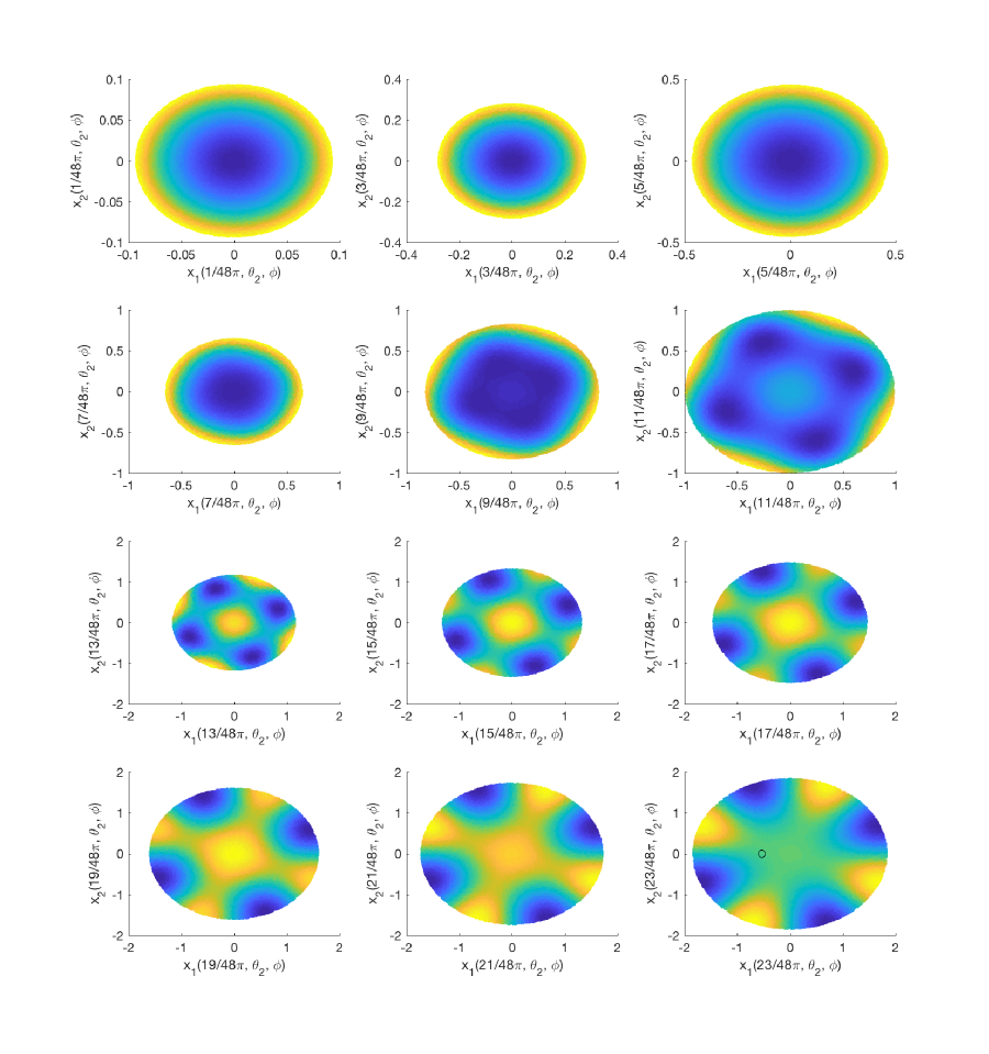
Figure 1: Visualization of the symmetrized hyperspherical harmonic $\accentset{\therefore}{Z}_{4}^{2}$ of the crystallograhic point group $1$ using the projection of the hyperangles onto the two-dimensional disk given by (4.8). For each panel, $\theta_{1}$ is fixed to a value in $\{\tfrac{1}{48}\pi,\tfrac{3}{48}\pi,\ldots,\tfrac{11}{48}\pi\}$, while $(\theta_{2},\phi)$ vary in $[0,\tfrac{\pi}{2}]\times[-\pi,\pi]$.

To illustrate the symmetries induced by the crystallographic group in the symmetrized hyperspherical harmonics we use a visualization described by Mason and Schuh, (2008). For a fixed hyperangle $(\theta_{1},\theta_{2},\phi)$, the functional value of $\accentset{\therefore}{Z}_{4}^{j}(\theta_{1},\theta_{2},\phi)$ is presented by using a projection of the hyperangle to an appropriate two-dimensional disk. More precisely, we project the hyperangle $(\theta_{1},\theta_{2},\phi)$ onto a two-dimensional disk by

$$P(\theta_{1},\theta_{2},\phi)=\begin{pmatrix}x_{1}(\theta_{1},\theta_{2},\phi)\\ x_{2}(\theta_{1},\theta_{2},\phi)\end{pmatrix}=\begin{pmatrix}R(\theta_{1},\theta_{2})\cos(\phi)\\ R(\theta_{1},\theta_{2})\sin(\phi)\end{pmatrix}\ ,$$ (4.8)

where the function $R(\theta_{1},\theta_{2})$ is given by

$$R(\theta_{1},\theta_{2})=(3/2)^{1/3}(\theta_{1}-\sin(\theta_{1})\cos(\theta_{1}))^{1/3}\sqrt{2(1-|\cos(\theta_{2})|)}.$$

For instance the angle $(\theta_{1},\theta_{2},\phi)=(\tfrac{11}{48}\pi,\tfrac{\pi}{4},\pi)$ is projected onto the point $(x_{1},x_{2})=(-0.5323,0)$. In Figure 1 we display the value (represented by an appropriate color) of the symmetrized harmonic $\accentset{\therefore}{Z}_{4}^{2}$ of the crystallographic group $1$ as a function of the coordinates $(x_{1}(\theta_{1},\theta_{2},\phi),x_{2}(\theta_{1},\theta_{2},\phi))$. In each of the twelve panels of Figure 1, $\theta_{1}$ is fixed to one of the values $\tfrac{1}{48}\pi,\tfrac{3}{48}\pi,\ldots,\tfrac{11}{48}\pi$, while the angles $\theta_{2}$ and $\phi$ vary between $[0,\pi/2]$ and $[-\pi,\pi]$, respectively. For instance, the value of $\accentset{\therefore}{Z}_{4}^{j}(\theta_{1},\theta_{2},\phi)$ at the hyperangle $(\theta_{1},\theta_{2},\phi)=(\tfrac{11}{48}\pi,\tfrac{\pi}{4},\pi)$ is presented in the bottom right panel in a light green color (see the black circle in the bottom right panel of Figure 1).

We now investigate the efficiency of the optimal design for the estimation of the coefficients in the regression model (2.1) with the hyperspherical harmonics up to order $d=4$, that is, the vector of regression functions is given by

$$f^{T}=(Y_{0,0,0},Y_{1,0,0},\ldots,Y_{1,1,1},\ldots,Y_{4,4,-4},\ldots,Y_{4,4,4})^{T}.$$

The optimal design for this model has been determined in Example 3.1 and a tedious calculation shows that the design $\zeta_{1}^{*}\otimes\zeta_{2}^{*}\otimes\nu^{*}$ defined in (3.31) satisfies the general equivalence theorem in Section 7.20 of Pukelsheim, (2006). Consequently, this design is also $\Phi_{p}$-optimal in the regression model (2.1), where the vector of regression functions is given by the symmetrized hyperspherical harmonics defined in (4.7), which correspond to the crystallographic point group $1$.
For the crystallographic point group $2$ there are $7$ symmetrized hyperspherical harmonics up to order $d=4$ consisting of a subset of the functions given in (4.6). These symmetrized hyperspherical harmonics define a linear regression model of the form (2.1), where the vector of regression functions $f_{2}$ is given by

$$f_{2}^{T}=(\accentset{\therefore}{Z}_{0}^{1},\accentset{\therefore}{Z}_{4}^{1},\accentset{\therefore}{Z}_{4}^{2},\accentset{\therefore}{Z}_{4}^{5},\accentset{\therefore}{Z}_{4}^{8},\accentset{\therefore}{Z}_{4}^{9},\accentset{\therefore}{Z}_{4}^{10})^{T}.$$ (4.9)

In the case of the crystallographic point group $2$ the design $\zeta_{1}^{*}\otimes\zeta_{2}^{*}\otimes\nu^{*}$ defined by (3.31) is not $\Phi_{p}$-optimal. However, using particle swarm optimization [see Clerc, (2006) for details] we determined the $D$-efficiency of the design $\zeta_{1}^{*}\otimes\zeta_{2}^{*}\otimes\nu^{*}$ numerically which is given by $81\%$. We also investigate the performance of the designs $\hat{\zeta}_{1}\otimes\hat{\zeta}_{2}\otimes\hat{\nu}$ and $\tilde{\zeta}_{1}\otimes\tilde{\zeta}_{2}\otimes\tilde{\nu}$ defined in equation (3.32) and (3.33) of Example 3.1. The $D$-efficiencies of these two designs are given by $59.38\%$ and $74.59\%$, respectively. Recall that the latter design uses the same support points as the optimal design. Our calculations show that the design $\zeta_{1}^{*}\otimes\zeta_{2}^{*}\otimes\nu^{*}$ in (3.31) provides reasonable efficiencies for estimating the coefficients in the regression model (2.1) with symmetrized hyperspherical harmonics with respect to the crystallographic point group $2$, whereas the uniform design $\hat{\zeta}_{1}\otimes\hat{\zeta}_{2}\otimes\hat{\nu}$ should not be used in this case.

Appendix A A Technical Result

A.1 Proof of Lemma 3.1

Assume that conditions (A) and (B) are satisfied and let $Q(x)$ be an arbitrary polynomial of degree z. The polynomial $Q$ can be represented in the form

$$Q(x)=P(x)V_{r}(x)+R(x),$$

where $V_{r}(x)=\prod_{j=1}^{r}(x-x_{j})$ is of degree $r$, the polynomial $P(x)$ is of degree $z-r$ and the polynomial $R(x)$ is of degree less than $r$. Since $x_{1},\ldots,x_{r}$ are the zeros of $V_{r}(x)$ we have that $Q(x_{j})=R(x_{j})$ for all $j=1,\ldots,r$ and furthermore, because the degree of $R(x)$ is at most $r-1$, it can be represented as

$$R(x)=\sum_{j=1}^{r}\ell_{j}(x)R(x_{j}).$$

Then from conditions (A) and (B) we obtain that

$$\int_{-1}^{1}a(x)Q(x)\,dx =\int_{-1}^{1}a(x)R(x)\,dx=\sum_{j=1}^{r}R(x_{j})\int_{-1}^{1}a(x)\ell_{j}(x)\,dx$$

$$=\sum_{j=1}^{r}R(x_{j})\tilde{a}\omega_{j}=\tilde{a}\sum_{j=1}^{r}\omega_{j}Q(x_{j}).$$

Using $Q(x)=x^{\ell}$, $\ell=0,\ldots,z$ yields the identities in (3.16) and for $\ell=0$ we obtain the expression $\tilde{a}=\int_{-1}^{1}a(x)\,dx$.

Now assume that (3.16) is valid. For $\ell=0,\ldots,z-r$ we have that

$$\int_{-1}^{1}V_{r}(x)a(x)x^{\ell}\,dx=\tilde{a}\sum_{j=1}^{r}\omega_{j}V_{r}(x_{j})x_{j}^{\ell}=0,$$

which gives condition (A). By noting that $\ell_{j}(x_{k})=\delta_{jk}$ we get that

$$\frac{1}{\tilde{a}}\int_{-1}^{1}a(x)\ell_{j}(x)\,dx=\sum_{k=1}^{r}\omega_{k}\ell_{j}(x_{k})=\sum_{k=1}^{r}\omega_{k}\delta_{jk}=\omega_{j},$$

which gives condition (B).

References

- Abrial et al., (2008) Abrial, P., Moudden, Y., Starck, J.-L., Fadili, J., Delabrouille, J., and Nguyen, M. K. (2008). CMB data analysis and sparsity. Statistical Methodology, 5(4):289–298.
- Alfed et al., (1996) Alfed, P., Neamtu, M., and Schumaker, L. L. (1996). Fitting scattered data on sphere-like surfaces using spherical splines. Journal of Computational and Applied Mathematics, 73(1-2):5–43.
- Andrews et al., (1991) Andrews, G., Askey, R., and Roy, R. (1991). Special Functions. Cambrdge Univ. Press.
- Avery and Wen, (1982) Avery, J. and Wen, Z.-Y. (1982). Angular integrations in -dimensional spaces and hyperspherical harmonics. International Journal of Quantum Chemistry, 22:717–738.
- Baldi et al., (2009) Baldi, P., Kerkyacharian, G., Marinucci, D., and Picard, D. (2009). Asymptotics for spherical needlets. Annals of Statistics, 37(3):1150–1171.
- Bunge, (1993) Bunge, H. J. (1993). Texture Analysis in Material Science: Mathematical Methods, 1st. ed. Cuvillier Verlag, Göttingen.
- Chang et al., (2000) Chang, T., Ko, D., Royer, J.-Y., and Lu, J. (2000). Regression techniques in plate tectonics. Statistical Science, 15(4):342–356.
- Chapman et al., (1995) Chapman, G. R., Chen, C., and Kim, P. T. (1995). Assessing geometric integrity through spherical regression techniques. Statistica Sinica, 5:173–220.
- Cheng, (1987) Cheng, C. S. (1987). An application of the Kiefer-Wolfowitz equivalence theorem to a problem in Hadamard transform optics. Annals of Statistics, 15(4):1593–1603.
- Clerc, (2006) Clerc, M. (2006). Particle Swarm Optimization. Iste Publishing Company, London.
- Dette and Melas, (2003) Dette, H. and Melas, V. B. (2003). Optimal designs for estimating individual coefficients in Fourier regression models. Annals of Statistics, 31(5):1669–1692.
- Dette et al., (2005) Dette, H., Melas, V. B., and Pepelyshev, A. (2005). Optimal designs for 3D shape analysis with spherical harmonic descriptors. Annals of Statistics, 33:2758–2788.
- Dette and Studden, (1993) Dette, H. and Studden, W. J. (1993). Geometry of -optimality. Annals of Statistics, 21(1):416–433.
- Dette and Wiens, (2009) Dette, H. and Wiens, D. P. (2009). Robust designs for 3D shape analysis with spherical harmonic descriptors. Statistica Sinica, 19:83–102.
- Di Marzio et al., (2009) Di Marzio, M., Panzera, A., and Taylor, C. C. (2009). Local polynomial regression for circular predictors. Statistics & Probability Letters, 79(1):2066–2075.
- Di Marzio et al., (2014) Di Marzio, M., Panzera, A., and Taylor, C. C. (2014). Nonparametric regression for spherical data. Journal of the American Statistical Association, 109(506):748–763.
- Dokmanić and Petrinović, (2010) Dokmanić, I. and Petrinović, D. (2010). Convolution on the n-sphere with application to PDF modeling. IEEE Transactions on Signal Processing, 58(3):1157–1170.
- Fedorov, (1972) Fedorov, V. V. (1972). Theory of Optimal Experiments. Academic Press, New York.
- Filová et al., (2011) Filová, L., Harman, R., and Klein, T. (2011). Approximate e-optimal designs for the model of spring balance weighing with a constant bias. Journal of Statistical Planning and Inference, 141(7):2480 – 2488.
- Genovese et al., (2004) Genovese, C. R., Miller, C. J., Nichol, R. C., Arjunwadkar, M., and Wasserman, L. (2004). Nonparametric inference for the cosmic microwave background. Statistical Science, 19(2):308–321.
- Harman, (2004) Harman, R. (2004). Minimal efficiency of designs under the class of orthogonally invariant information criteria. Metrika, 60(2):137–153.
- Hosseinbor et al., (2013) Hosseinbor, A. P., Chung, M. K., Schaefer, S. M., van Reekum, C. M., Peschke-Schmitz, L., Sutterer, M., Alexander, A. L., and Davidson, R. J. (2013). D hyperspherical harmonic (HyperSPHARM) representation of multiple disconnected brain subcortical structures. Medical Image Computing and Computer-Assisted Intervention, 16:598–605.
- Karlin and Studden, (1966) Karlin, S. and Studden, W. J. (1966). Tchebysheff Systems: With Application in Analysis and Statistics. Wiley, New York.
- Kiefer, (1974) Kiefer, J. (1974). General equivalence theory for optimum designs (approximate theory). The Annals of Statistics, 2(5):849–879.
- Kitsos et al., (1988) Kitsos, C. P., Titterington, D. M., and Torsney, B. (1988). An optimal design problem in rhythmometry. Biometrics, 44:657–671.
- Krivec, (1998) Krivec, R. (1998). Hyperspherical-harmonics methods for few-body problems. Few-Body Systems, 25:199–238.
- Lau and Studden, (1985) Lau, T.-S. and Studden, W. J. (1985). Optimal designs for trigonometric and polynomial regression using canonical moments. Annals of Statistics, 13(1):383–394.
- Lombardi et al., (2016) Lombardi, A., Palazzetti, F., Aquilanti, V., Grossi, G., Albernaz, A. F., Barreto, P. R. P., and Cruz, A. C. P. S. (2016). Spherical and hyperspherical harmonic representation of van der Waals aggregates. International Conference of Computational Methods in Sciences and Engineering, 1790(1):020005.
- Marinucci and Peccati, (2011) Marinucci, D. and Peccati, G. (2011). Random Fields on the Sphere: Representation, Limit Theorems and Cosmological Applications. London Mathematical Society Lecture Note Series. Cambridge University Press.
- Mason, (2009) Mason, J. K. (2009). The relationship of the hyperspherical harmonics to , and orientation distribution functions. Acta Crystallographica Sec. A., 65:259–266.
- Mason and Schuh, (2008) Mason, J. K. and Schuh, C. A. (2008). Hyperspherical harmonics for the representation of crystallographic texture. Acta Materialia, 56(20):6141–6155.
- Meremianin, (2009) Meremianin, A. V. (2009). Hyperspherical harmonics with arbitrary arguments. Journal of Mathematical Physics, 50(1):013526.
- Monnier, (2011) Monnier, J.-B. (2011). Nonparametric regression on the hyper-sphere with uniform design. TEST, 20(2):412–446.
- Narcowich et al., (2006) Narcowich, F. J., Petrushev, P., and Ward, J. D. (2006). Localized tight frames on spheres. SIAM Journal on Mathematical Analysis, 38:574–594.
- Patala et al., (2012) Patala, S., Mason, J. K., and Schuh, C. A. (2012). Improved representations of misorientation information for grain boundary science and engineering. Progress in Materials Science, 57(8):1383 – 1425.
- Patala and Schuh, (2013) Patala, S. and Schuh, C. A. (2013). Representation of single-axis grain boundary functions. Acta Materialia, 61(8):3068 – 3081.
- Pukelsheim, (2006) Pukelsheim, F. (2006). Optimal Design of Experiments. SIAM, Philadelphia.
- Pukelsheim and Rieder, (1992) Pukelsheim, F. and Rieder, S. (1992). Efficient rounding of approximate designs. Biometrika, 79:763–770.
- Schaeben and van den Boogaart, (2003) Schaeben, H. and van den Boogaart, K. G. (2003). Spherical harmonics in texture analysis. Tectonophysics, 370:253–268.
- Shin et al., (2007) Shin, H. H., Takahara, G. K., and Murdoch, D. J. (2007). Optimal designs for calibration of orientations. Canadian Journal of Statistics, 35(3):365–380.
- Silvey, (1980) Silvey, S. D. (1980). Optimal design. Chapman and Hall, London, London-New York.
- Vilenkin, (1968) Vilenkin, N. J. (1968). Special Functions and the Theory of Group Representations, volume 22. Translations of Mathematical Monographs, American Mathematical Society, Providence, RI.
- Wahba, (1981) Wahba, G. (1981). Spline interpolation and smoothing on the sphere. SIAM Journal on Scientific and Statistical Computing, 2(1):5–16.
- Wen and Avery, (1985) Wen, Z.-Y. and Avery, J. (1985). Some properties of hyperspherical harmonics. Math. Phys., 29:396–403.
- Zheng et al., (1995) Zheng, A., Doerschuk, P. C., and Johnson, J. E. (1995). Determination of three-dimensional low-resolution viral structure from solution x-ray scattering data. Biophysical Journal, 69(2):619–639.