Jeans type instability of a complex self-interacting scalar field in general relativity

Abstract

We study the gravitational instability of a general relativistic complex scalar field with a quartic self-interaction in an infinite homogeneous static background. This quantum relativistic Jeans problem provides a simplified framework to study the formation of the large-scale structures of the Universe in the case where dark matter is made of a scalar field. The scalar field may represent the wave function of a relativistic self-gravitating Bose-Einstein condensate. Exact analytical expressions for the dispersion relation and Jeans length $\lambda_{J}$ are obtained from a hydrodynamical representation of the Klein-Gordon-Einstein equations [Suárez and Chavanis, Phys. Rev. D 92, 023510 (2015)]. We compare our results with those previously obtained with a simplified relativistic model [Khlopov, Malomed and Y. B. Zeldovich, Mon. Not. R. astr. Soc. 215, 575 (1985)]. When relativistic effects are fully accounted for, we find that the perturbations are stabilized at very large scales of the order of the Hubble length $\lambda_{H}$. Numerical applications are made for ultralight bosons without self-interaction (fuzzy dark matter), for bosons with a repulsive self-interaction, and for bosons with an attractive self-interaction (QCD axions and ultralight axions). We show that the Jeans instability is inhibited in the ultrarelativistic regime (early Universe and radiationlike era) because the Jeans length is of the order of the Hubble length ($\lambda_{J}\sim\lambda_{H}$), except when the self-interaction of the bosons is attractive. By contrast, structure formation can take place in the nonrelativistic regime (matterlike era) for $\lambda_{J}\leq\lambda\leq\lambda_{H}$. Since the scalar field has a nonzero Jeans length due to its quantum nature (Heisenberg uncertainty principle or quantum pressure due to the self-interaction of the bosons), it appears that the wave properties of the scalar field can stabilize gravitational collapse at small scales, providing halo cores and suppressing small-scale linear power. This may solve the CDM crisis such as the cusp problem and the missing satellite problem. We also compare our results with those obtained in the case where dark matter is made of fermions instead of bosons.

I Introduction: A brief review

The formation of the large-scale structures of the Universe is an important problem of cosmology. In order to explain the evolution of cosmic structures, one must understand the mechanism that translates the almost homogeneous and isotropic early Universe revealed by the cosmic microwave background (CMB) radiation to the greatly clustered Universe observed today.

The clumping of matter resulting from the gravitational attraction acting on an initially uniform medium was first suggested by Newton in 1692 in a famous letter to the Reverend Dr. Bentley newton . He wrote: “But if the matter was evenly disposed throughout an infinite space, it could never convene into one mass; but some of it would convene into one mass and some into another, so as to make an infinite number of great masses, scattered at great distances from one to another throughout all that infinite space. And thus might the sun and fixt stars be formed, supposing the matter were of a lucid nature.”

The first serious theory of galaxy formation was proposed by Jeans in 1902 in a paper entitled “The Stability of a Spherical Nebula” jeans1902 . He supposed the Universe to be filled with a fluid with mass density $\rho$, pressure $P$ and velocity ${\bf v}$, and used classical hydrodynamic equations within the framework of Newtonian gravity. In the last part of his paper, he studied the gravitational instability of an infinite and spatially uniform gas and treated the question of the formation of self-gravitating objects by means of the interplay between the gravitational attraction and the pressure forces acting on a mass of gas. By linearizing the fluid equations about a static homogeneous state and decomposing the perturbations in Fourier modes of the form $\delta\rho({\bf r},t)\sim{\rm exp}[i({\bf k}\cdot{\bf r}-\omega t)]$, he obtained the dispersion relation

$$\omega^{2}=c_{s}^{2}k^{2}-4\pi G\rho,$$ (1)

where $c_{s}^{2}=P^{\prime}(\rho)$ is the square of the speed of sound in the medium. This equation exhibits a characteristic wavenumber

$$k_{J}=\left(\frac{4\pi G\rho}{c_{s}^{2}}\right)^{1/2}$$ (2)

called the Jeans wavenumber. The Jeans length $\lambda_{J}=2\pi/k_{J}$ gives an estimate of the minimum size of the objects that can undergo gravitational collapse. Perturbations for which the wavelength $\lambda$ is larger than the Jeans length $\lambda_{J}$ (i.e. $\lambda>\lambda_{J}$ or $k<k_{J}$) can grow by gravitational instability to form the structures observed in the Universe. According to Jeans’ study, the perturbations grow exponentially rapidly with a growth rate $\sigma(k)=\sqrt{-\omega(k)^{2}}$ where $\omega(k)$ is given by Eq. (1). The maximum growth rate

$$\sigma_{\rm max}=\sqrt{4\pi G\rho}$$ (3)

corresponds to a wavenumber

$$k_{*}=0\qquad{\rm i.e.}\qquad\lambda_{*}\rightarrow+\infty.$$ (4)

On the other hand, perturbations for which the wavelength $\lambda$ is smaller than the Jeans length $\lambda_{J}$ (i.e. $\lambda<\lambda_{J}$ or $k>k_{J}$) oscillate with a pulsation $\omega(k)$ like gravity-modified sound waves. Therefore, structure formation is suppressed on scales smaller than the Jeans length, and allowed on larger scales. The Jeans length $\lambda_{J}$ and the corresponding Jeans mass

$$M_{J}=\frac{4}{3}\pi\rho\left(\frac{\lambda_{J}}{2}\right)^{3}$$ (5)

determine the minimum size and the minimum mass above which a perturbation is amplified by self-gravity (they correspond to the condition of marginal stability $\omega=0$).

The Jeans study jeans1902 ; jeansbook has been extended in several directions. It can be applied to star formation in clouds of interstellar gas and to galaxy formation. The effect of a uniform rotation and a uniform magnetic field on the Jeans criterion has been treated by Chandrasekhar chandramagn ; chandramagnbook . The generalization of the Jeans criterion to infinite uniform rotating collisionless stellar systems described by the Vlasov equation has been treated by Lynden-Bell lbjeans . The computation of the Jeans length is the standard starting point for studying gravitational collapse. Even though today processes of stellar formation and galaxy formation are known with precision, the Jeans theory remains a good first approximation and has some pedagogical virtue. We refer to chavanisjeans for a review of the Jeans instability problem for collisional gaseous systems described by the Euler-Poisson equations and for collisionless stellar systems described by the Vlasov-Poisson equations.

The Jeans stability analysis encounters several problems. Firstly, the background state that is slightly perturbed in Jeans’ analysis, namely an infinite homogeneous distribution of matter, is not a steady state of the hydrodynamic equations. Therefore, the problem is mathematically ill-posed at the start even though the linearized equations for the perturbations make sense. This is what Binney and Tremaine bt call the “Jeans swindle”. Secondly, the results of Eqs. (3) and (4) suggest that there is no upper limit to the Jeans instability since the maximum growth rate is achieved for $\lambda_{*}\rightarrow+\infty$. Thirdly, as noted by Weinberg weinbergbook , the Jeans analysis is not rigorously applicable to the formation of galaxies in an expanding Universe because Jeans assumed a static medium whereas the rate of expansion of the Universe with a scale factor $a(t)$ is given by the Hubble parameter

$$H=\frac{\dot{a}}{a}=\left(\frac{8\pi G\rho}{3}\right)^{1/2}$$ (6)

which is of the same order as the maximum growth rate given by Eq. (3). Therefore, we cannot assume that the Universe is static, or even quasistatic, when doing the Jeans analysis. A last limitation of the original Jeans stability analysis is that it applies to nonrelativistic systems described by Newtonian gravity while the evolution of the Universe is fundamentally relativistic even though the Newtonian approximation is relevant in most situations of astrophysical interest.

The first satisfactory theory of the instabilities in an expanding Universe was given by Lifshitz lifshitz in 1946 using general relativity. He showed that disturbances at wavelengths above $\lambda_{J}$ grow, not exponentially, but like a power of $t$. Taking into account the expansion of the Universe is the correct manner to avoid the Jeans swindle. It leads, however, to different results. A nonrelativistic treatment of the instabilities in an expanding Universe was given by Bonnor bonnor in 1957 using a Newtonian world-model. He obtained the equation

$$\frac{d^{2}\delta_{k}}{dt^{2}}+2H\frac{d\delta_{k}}{dt}+\biggl{(}\frac{c_{s}^{2}}{a^{2}}k^{2}-{4\pi G\rho_{b}}\biggr{)}\delta_{k}=0,$$ (7)

where $\delta=\delta\rho/\rho$ is the density contrast and $k$ denotes here the comoving wavenumber (sometimes noted $k^{c}$). For a static Universe, one recovers the Jeans dispersion relation of Eq. (1) by setting $a={\rm cte}$ and introducing the physical wavenumber $k=k^{c}/a$. Equation (7) is the fundamental differential equation that governs the growth or decay of gravitational condensations in an expanding Universe. The case of collisionless stellar systems described by the Vlasov equation in an expanding Universe has been treated by Gilbert gilbert in Newtonian gravity. Further developments of these works for nonrelativistic and relativistic fluids, and for collisionless stellar systems, can be found in the books of Weinberg weinbergbook , Peebles peeblesbook , and Padmanabhan paddy .

In the previous studies, the Universe is treated as a classical fluid so that the Planck constant $\hbar$ does not appear in the equations. However, at very high energies, a standard hydrodynamical description of matter is not valid anymore. Rather, we expect that matter will be described in terms of quantum fields. In many particle physics models, scalar fields (SF) are introduced. Their role is to break high energy symmetries and to give mass to the particles by the mechanism of spontaneous symmetry breaking goldstone ; higgs ; weinbergmass . These SFs are described by the Klein-Gordon-Einstein (KGE) equations. A SF can be self-interacting, and this self-interaction is described by a potential $V(\varphi)$ coleman ; weinberg . It was soon realized that due to the potential $V(\varphi)$, SFs can play an important role in cosmology. In particular, if $\varphi$ is homogeneous in space, and trapped in a local minimum of the potential, the scale factor of the Universe expands exponentially rapidly. This leads to a primordial de Sitter era corresponding to what has been called inflation starobinsky ; guth ; linde1 ; hm ; as ; astw ; linde2 ; hawking ; linde3 . A detailed treatment of the evolution of a SF in the early Universe is performed in belinsky ; piran . It is shown that a real SF undergoes a stiff matter era followed by an inflation era which is an attractor of the KGE equations. Finally, it oscillates about the minimum of the potential and behaves in average as radiation and, later, as pressureless matter.

After the discovery of the acceleration of the Universe riess1 ; perlmutter ; riess2 , SFs were introduced as dark energy (DE) models. This led to the concepts of quintessence quintessence , Chaplygin gas model chaplygin , tachyons tachyon , phantom fields phantom , Galileon model galileon , polytropic polytropic , quadratic quadratic and logotropic logotropic models etc.

SFs have also been introduced in the context of dark matter (DM) to solve the cold dark matter (CDM) small-scale crisis such as the cusp problem burkert ; cusp , missing satellite problem miss1 ; miss2 , and too big to fail problem tbtf . Indeed, the wave properties of the SF can stabilize gravitational collapse, providing halo cores and suppressing small-scale structures (or linear power). Current works in particle physics and cosmology have suggested different kinds of SF candidates for a solution to the DM problem. Although these SFs have not yet been detected they are important DM candidates. They could undergo Jeans instability and form boson stars and/or DM halos as detailed below.

One possible DM candidate in cosmology is the axion preskill ; abbott ; dine ; turner1 ; davis . Unlike the Higgs boson, axions are sufficiently long-lived to coalesce into DM halos which constitute the seeds of galaxy formation. Axions are hypothetical pseudo-Nambu-Goldstone bosons of the Peccei-Quinn pq phase transition associated with a $U(1)$ symmetry that solves the strong charge parity (CP) problem of quantum chromodynamics (QCD). Axions also appear in string theory witten leading to the notion of string axiverse axiverse . The QCD axion is a spin-$0$ particle with a very small mass $m=10^{-4}\,{\rm eV}/c^{2}$ and an extremely weak self-interaction $a_{s}=-5.8\times 10^{-53}\,{\rm m}$ (where $a_{s}$ is the scattering length) arising from nonperturbative effects in QCD. Axions are extremely nonrelativistic and have huge occupation numbers, so they can be described by a classical field. Axionic dark matter can form a Bose-Einstein condensate (BEC) during the radiation-dominated era. Axions can thus be described by a relativistic quantum field theory with a real scalar field $\varphi$ whose evolution is governed by the KGE equations. In the nonrelativistic limit, they can be described by an effective field theory with a complex scalar field $\psi$ whose evolution is governed by the Gross-Pitaevskii-Poisson (GPP) equations. In that case, the SF describes the wave function of the BEC. One particularity of the axion is to have an attractive self-interaction ($a_{s}<0$).

The evolution of a Universe dominated by a cosmological SF that could represent an axion field was studied by Turner turner . He considered a real self-interacting SF described by the KGE equations with a potential of the form $V(\varphi)=a\varphi^{n}$ in an isotropic and homogeneous cosmology. He showed that the SF experiences damped oscillations but that, in average, it is equivalent to a perfect fluid with an equation of state $P=[(n-2)/(n+2)]\epsilon$. For $n=2$, the SF behaves as pressureless matter ($P=0$), and for $n=4$ it behaves as radiation ($P=\epsilon/3$) when the self-interaction is repulsive. Turner turner also mentioned the possibility of a stiff equation of state ($P=\epsilon$). The formation of structures in an axion-dominated Universe was investigated by Hogan and Rees hr and Kolb and Tkachev kt ; kt2 . They found very dense structures that they called “axion miniclusters” or “axitons”. These axitons have a mass $M_{\rm axiton}\sim 10^{-12}\,M_{\odot}$ and a radius $R_{\rm axiton}\sim 1\,R_{\odot}\sim 10^{9}\,{\rm m}$. These pseudosoliton configurations form in the very early Universe due to the attractive self-interaction of the axions. In their work, self-gravity is neglected. Kolb and Tkachev kt ; kt2 mentioned the possibility to form boson stars by Jeans instability through Bose-Einstein relaxation in the gravitationally bound clumps of axions. In other words, axitons are expected to collapse and form boson stars when self-gravity becomes important. Kolb and Tkachev kt ; kt2 considered ordinary boson stars with a repulsive self-interaction such as those sudied in tkachev . However, since axions have an attractive self-interaction, one cannot directly apply the standard results on boson stars kaup ; rb ; colpi ; tkachev ; chavharko to these objects. The case of self-interacting boson stars with an attractive self-interaction, possibly representing axion stars, was considered only recently gu ; bb ; prd1 ; prd2 ; braaten ; davidson ; cotner ; bectcoll ; eby ; tkachevprl ; helfer ; dkr ; phi6 . The analytical expression of the maximum mass of Newtonian self-gravitating BECs with attractive self-interaction was first obtained in prd1 ; prd2 (see Appendix D.4). For QCD axions, this leads to a maximum mass $M_{\rm max}=6.5\times 10^{-14}\,M_{\odot}$ and a radius $R_{*}=3.3\times 10^{-4}\,R_{\odot}=230\,{\rm km}$ (the average density is $\rho_{\rm max}=2.54\,{\rm kg/m^{3}}$). These are the maximum mass and minimum radius of dilute miniaxion stars. Coincidentally, these miniaxion stars have a mass comparable to the mass of the axitons kt ; kt2 but their mechanism of formation is completely different since self-gravity plays a crucial role. Obviously, QCD axions cannot form giant BECs with the dimension of DM halos. By contrast, they may form mini axion stars (of the asteroid size) that could be the constituents of DM halos under the form of mini massive compact halo objects (mini MACHOs) bectcoll . However, in that case, they would essentially behave as CDM and would not solve the small-scale crisis of CDM.

Much bigger objects of the size of DM halos can be formed in the case where the bosons have an ultrasmall mass of the order of $m\sim 10^{-22}\,{\rm eV}/c^{2}$ (ultralight bosons) and a very small self-interaction. Their mass can be larger if they have a substantial repulsive self-interaction. At the scale of DM halos, Newtonian gravity can be used and the KGE equations can be replaced by the GPP equations. The possibility that DM halos are made of a SF representing a gigantic boson star described by the KGE or GPP equations has been proposed by several authors baldeschi ; membrado ; sin ; jisin ; leekoh ; schunckpreprint ; matosguzman ; sahni ; guzmanmatos ; fuzzy ; peebles ; goodman ; mu ; arbey1 ; silverman1 ; matosall ; silverman ; lesgourgues ; arbeycosmo ; arbey (see also fm1 ; bohmer ; fm2 ; bmn ; fm3 ; sikivie ; mvm ; lee09 ; ch1 ; leelim ; prd1 ; prd2 ; prd3 ; briscese ; harkocosmo ; harko ; abrilMNRAS ; aacosmo ; velten ; pires ; park ; rmbec ; rindler ; lora ; abrilJCAP ; mhh ; lensing ; glgr1 ; robles ; ch2 ; ch3 ; shapiro ; bettoni ; lora2 ; mlbec ; madarassy ; suarezchavanis1 ; suarezchavanis2 ; stiff ; guthnew ; souza ; freitas ; alexandre ; schroven ; pop ; martinez ; ebydm ; cembranos ; schwabe ; fan ; calabrese ; bectcoll ; chavmatos ; hui ; zhang ; total ; suarezchavanis3 ; shapironew for more recent works). A brief history of the SFDM/BECDM scenario can be found in the Introduction of prd1 and in revueabril ; revueshapiro ; bookspringer ; marshrevue .

This brief review shows that SFs play a very important role in particle physics, astrophysics and cosmology. When SFs are considered, quantum mechanics arises in the problem and the Planck constant $\hbar$ enters into the equations.

The gravitational instability of a spatially homogeneous SF in a static background in general relativity was first discussed by Khlopov et al. khlopov . They considered a real or complex SF and demonstrated its instability to be analogous to the Jeans instability of a classical self-gravitating gas in the sense that there is a critical wavelength above which the system becomes unstable. For a noninteracting SF, Khlopov et al. khlopov obtained a quantum Jeans wavenumber given by

$$k_{J}=\left(\frac{16\pi G\rho m^{2}}{\hbar^{2}}\right)^{1/4}.$$ (8)

They also considered a self-interacting SF with a quartic potential $V(|\varphi|^{2})=(\lambda/4\hbar c)|\varphi|^{4}$. They treated the case of repulsive interactions ($\lambda>0$) but also the case of attractive ones ($\lambda<0$) that arise in the Coleman-Weinberg model coleman for not too large fields. This corresponds to a $|\varphi|^{4}$ potential with the “wrong” sign. In that case, they showed that the quartic term develops an additional (besides gravitational) instability that they called “hydrodynamic” because it corresponds to a fluid with a negative pressure. This is a nongravitational instability of the SF.

Bianchi et al. bianchi generalized the work of Khlopov et al. khlopov for a noninteracting SF to a fully quantum context. They used this system to make self-gravitating structures from a SF in a coherent state of a superfluid. They interpreted the density perturbations of a cosmological quantum real SF as excitations of a BEC at vanishing temperature. They showed that the dispersion relation of the perturbations of the real SF obtained by Khlopov et al. khlopov matches the nonrelativistic Bogoliubov energy spectum bogoliubov of the excitations of bosonic ground states (valid for a general pair potential of interation $V_{k}$) when the potential of interaction is the gravitational one, $V_{k}=-4\pi Gm^{2}/k^{2}$. They mentioned that the physical mechanism that leads to a finite Jeans length has the same nature as that which accounts for the equilibrium of the boson stars rb .

Bianchi et al. bianchi also considered the growth of structures induced by a noninteracting SF in an expanding Universe. They first remarked that, in the expression of the Jeans wavenumber (8), the zero-point pressure plays the same role which, in the traditional Jeans treatment, is played by the pressure of a thermal gas in equilibrium against gravitational attraction. Formally, this means that the quantum Jeans wavenumber (8) can be obtained from the classical Jeans wavenumber (2) by making the substitution

$$c_{s}^{2}=\frac{\hbar^{2}k^{2}}{4m^{2}}.$$ (9)

Then, applying the linearized theory of perturbations for a classical fluid in general relativity developed by Lifshitz and Khalatnikov lk and Weinberg weinbergbook , and making the substitution from Eq. (9), they obtained, in the nonrelativistic limit (see Eq. (7)), the following equation

$$\frac{d^{2}\delta_{k}}{dt^{2}}+2H\frac{d\delta_{k}}{dt}+\biggl{(}\frac{\hbar^{2}k^{4}}{4m^{2}a^{4}}-{4\pi G\rho_{b}}\biggr{)}\delta_{k}=0$$ (10)

for the evolution of the density contrast. They contrasted this equation from the one obtained by Ipser and Sikivie is for a pressureless axion field in which the speed of sound vanishes (obtained from Eq. (7) with $c_{s}=0$). They also considered the ultra-relativistic limit of their model and showed that, in this case, the Jeans length is larger than the Hubble length (horizon) thereby preventing the growth of structures.

The study of perturbations and the growth of structures for a relativistic SF described by the KGE equations in an expanding background is complicated. It has been treated in several papers sasaki1 ; sasaki2 ; mukhanov ; ratrapeebles ; nambu ; ratra ; mukhanovrevue ; hwang ; jetzer ; hu ; joyce ; ma ; pb ; brax ; matos ; hn1 ; hn2 ; malik ; axiverse ; mf ; easther ; phn ; mmss ; nph ; nhp ; hlozek ; alcubierre1 ; cembranos ; ug ; marshrevue ; spintessence ; jk ; fm2 ; fm3 in different contexts where the SF can represent the inflaton or can model DM or DE. In these studies, the formation of structures in an expanding Universe is studied directly from the field equations for $\varphi$.

Instead of working in terms of field variables, a fluid approach can be adopted (see a brief history of this approach in the Introduction of chavmatos ). In the nonrelativistic case, this hydrodynamic approach was introduced by Madelung madelung who showed that the Schrödinger equation is equivalent to the Euler equations for an irrotational fluid with an additional quantum potential arising from the finite value of $\hbar$ accounting for Heisenberg’s uncertainty principle. This approach has been generalized to the GPP equations in the context of DM halos by fuzzy ; bohmer ; sikivie ; prd1 ; prd2 ; prd3 ; aacosmo ; rindler among others. In the relativistic case, de Broglie broglie1927a ; broglie1927b ; broglie1927c in his so-called pilot wave theory, showed that the KG equations are equivalent to hydrodynamic equations including a covariant quantum potential. This approach has been generalized to the Klein-Gordon-Poisson (KGP) and KGE equations in the context of DM halos by abrilMNRAS ; suarezchavanis1 ; suarezchavanis2 ; chavmatos (see also debbasch ; chavharko ; ns for BEC stars). In this hydrodynamic representation, DM halos result from the balance between the gravitational attraction and the quantum pressure arising from the Heisenberg uncertainty principle or from the self-interaction of the bosons. At small scales, quantum effects are important and can prevent the formation of singularities and solve the cusp problem and the missing satellite problem. At large scales, quantum effects are generally negligible (except in the early Universe) and one recovers the hydrodynamic equations of the $\Lambda$CDM model.

It is possible to study the Jeans instability problem directly from these hydrodynamic equations. This is closer in spirit to the original Jeans’ approach. In the relativistic regime, valid during the radiation era or earlier, one should use the fluid equations based on the KGE equations. In the nonrelativistic regime, appropriate to study structure formation in the matter era, the KGE equations reduce to the GPP equations or to the Schrödinger-Poisson equations, and one can use the corresponding fluid equations.

The Jeans instability of a nonrelativistic SF was qualitatively discussed by Hu et al. fuzzy who rederived the quantum Jeans length of Eq. (8). A more detailed analysis was done by Sikivie and Yang sikivie who considered the growth of structures in an expanding Universe and rederived Eq. (10) directly from the quantum hydrodynamic equations. In that case, the term $\hbar^{2}k^{4}/4m^{2}a^{2}$ arises directly from the quantum potential in the Euler equation, and there is no need to make the formal (and mathematically illicit) substitution from Eq. (9). In these studies, the SF is assumed to be noninteracting. The Jeans instability of a nonrelativistic SF with an arbitrary self-interaction (repulsive or attractive) in a static Universe has been treated in detail by prd1 who derived the Jeans length of Eq. (34) below. The growth of structures of a self-interacting SF in an expanding Universe was treated independently by abrilMNRAS and aacosmo who derived the equation

$$\frac{d^{2}\delta_{k}}{dt^{2}}+2H\frac{d\delta_{k}}{dt}+\biggl{(}\frac{\hbar^{2}k^{4}}{4m^{2}a^{4}}+\frac{c_{s}^{2}}{a^{2}}k^{2}-{4\pi G\rho_{b}}\biggr{)}\delta_{k}=0$$

(11)

for the evolution of the density contrast. For $\hbar=0$, one recovers the classical Bonnor equation (7) and for $c_{s}=0$ one recovers Eq. (10) as particular case.

The study of the Jeans instability of a relativistic complex SF with a quartic potential based on the hydrodynamic approach has been initiated in our previous paper suarezchavanis1 . Preliminary results were given for a static Universe. In particular, we obtained the dispersion relation of Eq. (58) and the Jeans length of Eq. (65). The case of an expanding Universe was also considered in suarezchavanis1 . Using simplifying approximations, which amount to neglecting some relativistic terms while preserving the exact expression of the static Jeans length, we obtained the equation

$$\frac{d^{2}\delta_{k}}{dt^{2}}+2H\frac{d\delta_{k}}{dt}+\biggl{[}\frac{\hbar^{2}k^{4}}{4m^{2}a^{4}}+\frac{c_{s}^{2}}{a^{2}}k^{2}$$

$$-\frac{4\pi G\rho_{b}}{1+\frac{3H^{2}a^{2}}{k^{2}c^{2}}}\left(1+\frac{2c_{s}^{2}}{c^{2}}\right)\left(1+\frac{3c_{s}^{2}}{c^{2}}+\frac{\hbar^{2}k^{2}}{4m^{2}c^{2}a^{2}}\right)\biggr{]}\delta_{k}=0$$

(12)

for the evolution of the density contrast. We showed that general relativity prevents the growth of perturbations whose wavelengths are larger than the Hubble length (horizon). More precisely, the SF gives three distinct regions in Fourier space. On scales smaller than the Jeans length $\lambda_{J}$, the contrast in the energy density oscillates with constant or growing amplitude (depending on the dominant regime, either noninteracting or nonquantum). Above the Jeans length $\lambda_{J}$ but still below the Hubble length $\lambda_{H}$, self-gravity prevails, the density contrast grows, and the Jeans instability comes into play. Lastly, at scales close to or larger than the Hubble length $\lambda_{H}$, the energy density freezes due to general relativistic effects. These results are consistent with those obtained in mukhanovbook using SF equations.

In this paper, we continue the work initiated in suarezchavanis1 . We consider a relativistic complex SF with a $|\varphi|^{4}$ self-interaction. The cosmological evolution of a homogeneous SF with a repulsive self-interaction has been treated in shapiro from field equations (see also the previous works of jetzer ; sj ; spintessence ; arbeycosmo ) and in suarezchavanis1 ; suarezchavanis3 from hydrodynamic equations. For weak self-interactions (in a sense detailed in suarezchavanis3 ), the SF undergoes a stiff matter era followed by a matterlike era. For stronger self-interactions, it undergoes a stiff matter era followed by a radiationlike era, and finally a matterlike era. Phase diagrams are provided in suarezchavanis3 . The case of a SF with an attractive self-interaction has also been considered in suarezchavanis3 leading to intriguing results. It appears that two evolutions, corresponding to two different branches, are possible. The SF behaves as DM on the normal branch and as DE on the peculiar branch. In the latter, the SF maintains a constant energy density as a result of spintessence spintessence .

In the present paper, we restrict ourselves to a static background and study the Jeans instability of a general relativistic complex SF with a $|\varphi|^{4}$ self-interaction. In Sec. II, we expose our procedure to solve the problem and refer to our previous work suarezchavanis1 for technical details. In Sec. III, we briefly recall the results of the Jeans instability of a nonrelativistic SF prd1 . In Sec. IV, we consider a simplified relativistic model, which turns out to be equivalent to the one considered by Khlopov et al. khlopov , where some terms are neglected in the dispersion relation. In Sec. V, we consider the exact relativistic model where all the terms are retained in the dispersion relation (the nongravitational limit is treated in Sec. VI). When relativistic effects are fully accounted for, we find that the perturbations are stabilized at very large scales of the order of the Hubble length $\lambda_{H}$. In the following sections, we consider astrophysical and cosmological applications of our theoretical results. In Sec. VII, we show that the Jeans instability is inhibited in the ultrarelativistic regime (early Universe and radiationlike era) because the Jeans length is of the order of the Hubble length ($\lambda_{J}\sim\lambda_{H}$), except when the self-interaction of the SF is attractive. In Sec. VIII, we show that the Jeans instability can take place in the nonrelativistic regime (matterlike era) for $\lambda_{J}\leq\lambda\leq\lambda_{H}$. Numerical applications are made for ultralight bosons without self-interaction (fuzzy dark matter), for bosons with a repulsive self-interaction, and for bosons with an attractive self-interaction (QCD axions and ultralight axions). In Sec. IX, we compare our results with those obtained in the case where dark matter is made of fermions instead of bosons.

II The Jeans instability of a relativistic complex SF

We consider a relativistic complex SF, possibly representing the wave function of a BEC at $T=0$, with a quartic self-interaction potential of the form

$$V_{\rm tot}(|\varphi|^{2})=\frac{m^{2}c^{2}}{2\hbar^{2}}|\varphi|^{2}+\frac{2\pi a_{s}m}{\hbar^{2}}|\varphi|^{4}.$$ (13)

The quadratic term is the rest-mass term and the quartic term is the self-interaction term. Here, $m$ denotes the mass of the bosons and $a_{s}$ their scattering length. The self-interaction is repulsive when $a_{s}>0$ and attractive when $a_{s}<0$ revuebec . The evolution of the SF is described by the KG equation

$$\Box\varphi+2\frac{dV_{\rm tot}}{d|\varphi|^{2}}\varphi=0,$$ (14)

where $\Box$ is the d’Alembertian operator in a curved spacetime:

$$\Box\equiv D_{\mu}(g^{\mu\nu}\partial_{\nu})=\frac{1}{\sqrt{-g}}\partial_{\mu}(\sqrt{-g}\,g^{\mu\nu}\partial_{\nu}).$$ (15)

For the specific SF potential (13), the KG equation takes the form

$$\square\varphi+\frac{m^{2}c^{2}}{\hbar^{2}}\varphi+\frac{8\pi a_{s}m}{\hbar^{2}}|\varphi|^{2}\varphi=0.$$ (16)

It is coupled to the Einstein equations

$$R_{\mu\nu}-\frac{1}{2}g_{\mu\nu}R=\frac{8\pi G}{c^{4}}T_{\mu\nu},$$ (17)

where $R_{\mu\nu}$ is the Ricci tensor and $T^{\mu\nu}$ is the energy-momentum tensor of the SF given by

$$T_{\mu\nu}=\frac{1}{2}(\partial_{\mu}\varphi^{*}\partial_{\nu}\varphi+\partial_{\nu}\varphi^{*}\partial_{\mu}\varphi)$$

$$-g_{\mu\nu}\left[\frac{1}{2}g^{\rho\sigma}\partial_{\rho}\varphi^{*}\partial_{\sigma}\varphi-V_{\rm tot}(|\varphi|^{2})\right].$$ (18)

Our aim is to study the Jeans instability of an infinite homogeneous relativistic complex SF in a static background in relation to the formation of structures in cosmology. Following our previous work suarezchavanis1 , we proceed as follows:

(i) We first introduce the Newtonian gauge [see Eq. (I-18)] to write the KGE equations in the weak field approximation [see Eqs. (I-20) and (I-26)]. Since we consider the linear perturbation regime, there is no limitation in using this gauge. However, we consider the simplest form of the Newtonian gauge, only taking into account scalar perturbations which are the ones that contribute to the formation of structures in cosmology. Vector contributions (which are supposed to be always small) vanish during cosmic inflation and tensor contributions (which account for gravitational waves) are neglected mukhanovrevue . We also neglect anisotropic stress for simplicity.

(ii) We make the Klein transformation [see Eq. (I-34)], which amounts to subtracting the rest mass energy, and obtain the general relativistic GPE equations [see Eqs. (I-35) and (I-36)] from the KGE equations. The interest of this transformation is that the GPE equations (unlike the KGE equations) have a well defined nonrelativistic limit $c\rightarrow+\infty$, leading to the GPP equations [see Eqs. (I-C1) and (I-C2)] that are relevant in the Newtonian regime.

(iii) We use the Madelung transformation [see Eqs. (I-39) and (I-40)] to obtain a hydrodynamic representation of the GPE equations. These hydrodynamic equations [see Eqs. (I-41)-(I-44)] are equivalent to the GPE equations (themselves equivalent to the KGE equations) and they put us in a situation similar to the one investigated by Jeans jeans1902 ; jeansbook except that we have additional terms due to quantum mechanics ($\hbar$) and relativity ($c$). These hydrodynamic equations depend on a pseudo rest-mass density defined by

$$\rho=\frac{m^{2}}{\hbar^{2}}|\varphi|^{2}=|\psi|^{2}.$$ (19)

It is only in the nonrelativistic limit $c\rightarrow+\infty$ that $\rho$ corresponds to the mass density, but we can always introduce $\rho$ from Eq. (19) as a convenient notation, even in the relativistic regime suarezchavanis1 .

(iv) The hydrodynamic equations involve a pseudo pressure given by the polytropic (quadratic) equation of state

$$p=\frac{2\pi a_{s}\hbar^{2}}{m^{3}}\rho^{2}.$$ (20)

This pressure is due to the self-interaction of the bosons. This equation of state keeps the same form in the nonrelativistic and relativistic regimes. From this equation of state, we can define the pseudo speed of sound

$$c_{s}^{2}=p^{\prime}(\rho)=\frac{4\pi a_{s}\hbar^{2}\rho}{m^{3}}.$$ (21)

We note that $c_{s}^{2}>0$ for a repulsive self-interaction and $c_{s}^{2}<0$ for an attractive self-interaction.

(v) We now consider the case of a static Universe corresponding to $a=1$ and $H=0$ in the equations of suarezchavanis1 . For the homogeneous background, we have the exact relations suarezchavanis1 :

$$\epsilon=\rho c^{2}\left(1+\frac{6\pi a_{s}\hbar^{2}}{m^{3}c^{2}}\rho\right),$$ (22)

$$\rho=\frac{m^{3}c^{2}}{12\pi a_{s}\hbar^{2}}\left(\sqrt{1+\frac{24\pi a_{s}\hbar^{2}}{m^{3}c^{4}}\epsilon}-1\right),$$ (23)

$$P=p=\frac{m^{3}c^{4}}{72\pi a_{s}\hbar^{2}}\left(\sqrt{1+\frac{24\pi a_{s}\hbar^{2}}{m^{3}c^{4}}\epsilon}-1\right)^{2}$$ (24)

between the (uniform) pseudo rest mass density $\rho$, the (uniform) energy density $\epsilon$, and the (uniform) pressure $P$. For a noninteracting SF ($a_{s}=0$), these relations reduce to

$$\epsilon=\rho c^{2},\qquad P=0,$$ (25)

in all the regimes (relativistic and nonrelativistic). We now have to distinguish attractive and repulsive self-interactions. We first consider repulsive self-interactions ($a_{s}>0$). In the ultrarelativistic limit $\rho\gg\rho_{R}=m^{3}c^{2}/6\pi a_{s}\hbar^{2}$ (see Appendix D.3), we get

$$\epsilon\sim\frac{6\pi a_{s}\hbar^{2}}{m^{3}}\rho^{2},\qquad P\sim\frac{1}{3}\epsilon.$$ (26)

This corresponds to the radiationlike era in shapiro ; suarezchavanis3 . Indeed, in the ultrarelativistic limit, the SF behaves like radiation at the background level. In the nonrelativistic limit $\rho\ll\rho_{R}$, we get

$$\epsilon\sim\rho c^{2},\qquad P\sim\frac{2\pi a_{s}\hbar^{2}}{m^{3}c^{4}}\epsilon^{2}.$$ (27)

This corresponds to the pressureless matterlike era in shapiro ; suarezchavanis3 . Indeed, in the nonrelativistic limit, the SF behaves as pressureless matter at the bakground level. We now consider attractive self-interactions ($a_{s}<0$). In the ultrarelativistic limit, coming back temporarily to the more realistic case of an expanding Universe, we know from the results of suarezchavanis3 that the pseudo rest-mass density tends to the value (see Appendix D.5):

$$\rho_{i}=\frac{m^{3}c^{2}}{12\pi|a_{s}|\hbar^{2}}.$$ (28)

We also have

$$\epsilon_{i}=\frac{m^{3}c^{4}}{24\pi|a_{s}|\hbar^{2}},\qquad P_{i}=-\frac{1}{3}\epsilon_{i}.$$ (29)

This corresponds to the cosmic stringlike era in suarezchavanis3 . In the nonrelativistic limit $\rho\ll\rho_{i}$, we recover Eq. (27).

(vi) We linearize the hydrodynamic equations about a spatially homogeneous state (making the Jeans swindle) and decompose the perturbation in Fourier modes of the form ${\rm exp}[i({\bf k}\cdot{\bf r}-\omega t)]$. In this way, we obtain the dispersion relation $\omega(k)$ that relates the complex pulsation $\omega$ to the wave number $k=2\pi/\lambda$. From this dispersion relation, we can determine the oscillatory modes ($\omega^{2}>0$), the growing modes ($\omega^{2}<0$) giving rise to a linear instability, the Jeans length $\lambda_{J}$ (corresponding to the neutral mode $\omega=0$) separting stable and unstable modes, and the optimal length $\lambda_{*}$ having the maximum growth rate $\sigma_{\rm max}$.

The general dispersion relation corresponding to the full KGE equations without approximation has been determined in our previous paper suarezchavanis1 , see Eq. (I-69), but only a preliminary analysis of its solutions was given. In the present paper, we study it in greater detail. To increase the complexity of the problem progressively, we first consider the nonrelativistic model (Sec. III), then a simplified relativistic model where some terms are neglected in the KGE equations (Sec. IV), and finally the exact relativistic model (Sec. V). In each section, we provide general equations valid for repulsive ($c_{s}^{2}>0$) and attractive ($c_{s}^{2}<0$) self-interactions but in the discussion, for simplicity, we restrict ourselves to repulsive self-interactions. The case of attractive self-interactions is considered in greater detail in the nongravitational limit (Sec. VI).

III The nonrelativistic model

In this section, we study the dispersion relation of a self-gravitating BEC in the nonrelativistic limit $c\rightarrow+\infty$. In that limit, the KGE equations reduce to the GPP equations [see Eqs. (I-C1) and (I-C2)]. The Jeans problem based on the hydrodynamic equations derived from the GPP equations [see Eqs. (I-C3)-(I-C6)] has been studied in detail in prd1 for both repulsive ($a_{s}>0$) and attractive ($a_{s}<0$) self-interactions between the bosons. In this section, we briefly recall the main results of this study (restricting ourselves to the case $a_{s}>0$) in order to facilitate the comparison with the relativistic results discussed in the following sections.

III.1 The general case

In the nonrelativistic limit, the dispersion relation characterizing the small perturbations of a spatially homogeneous self-gravitating BEC is given by (see Sec. V of prd1 ):

$$\omega^{2}=\frac{\hbar^{2}k^{4}}{4m^{2}}+c_{s}^{2}k^{2}-4\pi G\rho.$$ (30)

Equation (30) corresponds to the Bogoliubov energy spectrum of the excitations of a self-gravitating and weakly self-interacting BEC bogoliubov . The function $\omega^{2}(k)$ is plotted in Fig. 1 using the normalization of Appendix A.1 with $\chi\propto 2/c^{2}=0$ (nonrelativistic limit). It starts from $\omega^{2}(0)=-4\pi G\rho$ at $k=0$ and increases monotonically with $k$. For $k\rightarrow 0$, we obtain

$$\omega^{2}\simeq-4\pi G\rho+c_{s}^{2}k^{2},$$ (31)

corresponding to the classical regime. For $k\rightarrow+\infty$, we obtain

$$\omega^{2}\sim\frac{\hbar^{2}k^{4}}{4m^{2}},$$ (32)

corresponding to the strongly quantum regime.

Figure 1: Dispersion relation $\Omega^{2}(\kappa)$ of the nonrelativistic model ($\chi=0$) for different values of the speed of sound (self-interaction) $\alpha=0,1,2,3,4,5$.

The Jeans wavenumber $k_{J}$, corresponding to $\omega=0$, is determined by the equation

$$\frac{\hbar^{2}k_{J}^{4}}{4m^{2}}+c_{s}^{2}k_{J}^{2}-4\pi G\rho=0.$$ (33)

This is a second degree equation in $k_{J}^{2}$. Its physical solution (corresponding to a real Jeans wavenumber) is prd1 :

$$k_{J}^{2}=\frac{2m^{2}}{\hbar^{2}}\left(-c_{s}^{2}+\sqrt{c_{s}^{4}+\frac{4\pi G\rho\hbar^{2}}{m^{2}}}\right).$$ (34)

The Jeans wavenumber $k_{J}^{2}$ is plotted as a function of the speed of sound (self-interaction) $\alpha\propto c_{s}^{2}/2$ in Fig. 2 using the normalization of Appendix A.1. The system is stable ($\omega^{2}>0$) for $k>k_{J}$ and unstable ($\omega^{2}<0$) for $k<k_{J}$ (see Fig. 1). In the first case, the perturbations oscillate with a pulsation $\omega=\sqrt{\omega^{2}}$. In the second case, the perturbations grow exponentially rapidly with a growth rate $\sigma=\sqrt{-\omega^{2}}$. The maximum growth rate corresponds to $k_{*}=0$ (infinitely large scales) and is equal to

$$\sigma_{\rm max}=(4\pi G\rho)^{1/2}.$$ (35)

It is of the order of the inverse of the dynamical time $t_{D}=(4\pi G\rho)^{-1/2}$ bt . We note from Figs. 1 and 2 that the Jeans length increases with the speed of sound (self-interaction) while the maximum growth rate remains constant. Therefore, the self-interaction increases the Jeans length but does not change the maximum growth rate.

Figure 2: Jeans wavenumber $\kappa_{J}$ of the nonrelativistic model ($\chi=0$) as a function of the speed of sound $\alpha$ (self-interaction).

III.2 The noninteracting limit

In the noninteracting limit ($c_{s}=0$), the dispersion relation of Eq. (30) reduces to

$$\omega^{2}=\frac{\hbar^{2}k^{4}}{4m^{2}}-4\pi G\rho.$$ (36)

The Jeans wavenumber is given by

$$k_{J}^{2}=\left(\frac{16\pi G\rho m^{2}}{\hbar^{2}}\right)^{1/2}.$$ (37)

We call it the quantum Jeans wavenumber because it is due to the competition between the gravitational attraction and the repulsion due to the quantum pressure arising from the Heisenberg uncertainty principle.

III.3 The TF limit

In the TF limit in which the quantum potential can be neglected ($\hbar=0$), the dispersion relation of Eq. (30) reduces to

$$\omega^{2}=c_{s}^{2}k^{2}-4\pi G\rho.$$ (38)

This is the classical Jeans dispersion relation except that, in the present context, the pressure term is due to the self-interaction of the bosons instead of thermal motion (we recall that $T=0$ for our system). For $k\rightarrow+\infty$:

$$\omega^{2}(k)\sim c_{s}^{2}k^{2}.$$ (39)

For large wavenumbers (short wavelengths), the pressure term dominates the gravitational term and the waves behave as sound waves.

The Jeans wavenumber is given by

$$k_{J}^{2}=\frac{4\pi G\rho}{c_{s}^{2}}.$$ (40)

It results from the competition between the gravitational attraction and the repulsion due to the pressure arising from the self-interaction of the bosons. We call it the classical Jeans wavenumber because it is similar to the ordinary Jeans wavenumber obtained from a classical hydrodynamic approach. We recall, however, that, in the present context, the pressure due to the self-interaction of the bosons has an intrinsic quantum nature.

Remark: In the case $\hbar=c_{s}=0$, the dispersion relation of Eq. (30) reduces to $\omega^{2}=-4\pi G\rho$. The system is unstable at all wavelengths and the growth rate has a constant value $\sigma=(4\pi G\rho)^{1/2}$.

IV The simplified relativistic model

In this section, we consider a simplified relativistic model which corresponds to the weak field limit $\Phi/c^{2}\rightarrow 0$ of the KGE equations (see Appendix D of suarezchavanis1 and Sec. 11 of suarezchavanis2 ). This is different from the nonrelativistic limit $c\rightarrow+\infty$ considered in the previous section. This model coincides with the one studied by Khlopov et al. khlopov . However, this model is not fully accurate because it neglects some terms in the linearized KGE equations (the terms $\Phi/c^{2}$ that are not multiplied by $c^{2}$). Actually, in the relativistic regime, one must take into account all the terms of order $\Phi/c^{2}$ in the linearized KGE equations. The exact relativistic model will be considered in Sec. V. However, we first consider this simplified model in order to compare it later with the exact one.

IV.1 The general case

In the simplified relativistic model, the dispersion relation is given by (see Appendix D of suarezchavanis1 ):

$$\frac{\hbar^{2}}{4m^{2}c^{4}}\omega^{4} - \biggl{(}1+\frac{3c_{s}^{2}}{c^{2}}+\frac{\hbar^{2}k^{2}}{2m^{2}c^{2}}\biggr{)}\omega^{2}+\frac{\hbar^{2}k^{4}}{4m^{2}}+c_{s}^{2}k^{2}$$ (41)

$$- 4\pi G\rho\left(1+\frac{2c_{s}^{2}}{c^{2}}\right)=0.$$

This is a second degree equation in $\omega^{2}$. The discriminant of this equation

$$\Delta=\left(1+\frac{3c_{s}^{2}}{c^{2}}\right)^{2}+\left(1+\frac{2c_{s}^{2}}{c^{2}}\right)\frac{\hbar^{2}k^{2}}{m^{2}c^{2}}$$

$$+\frac{\hbar^{2}}{m^{2}c^{4}}4\pi G\rho\left(1+\frac{2c_{s}^{2}}{c^{2}}\right)$$ (42)

is manifestly positive. Therefore, the dispersion relation has two real branches $\omega_{\pm}^{2}(k)$. For $k=0$:

$$\omega_{\pm}^{2}(0)=\frac{2m^{2}c^{4}}{\hbar^{2}}\Biggl{\{}1+\frac{3c_{s}^{2}}{c^{2}}\pm\Biggl{[}\left(1+\frac{3c_{s}^{2}}{c^{2}}\right)^{2}$$

$$+\frac{4\pi G\rho\hbar^{2}}{m^{2}c^{4}}\left(1+\frac{2c_{s}^{2}}{c^{2}}\right)\Biggr{]}^{1/2}\Biggr{\}}.$$ (43)

We note that $\omega_{+}^{2}(0)>0$ and $\omega_{-}^{2}(0)<0$. For $k\rightarrow 0$:

$$\omega_{\pm}^{2}(k)\simeq\omega_{\pm}^{2}(0)+c_{\rm eff}^{2}k^{2}.$$ (44)

The coefficient in front of $k^{2}$ can be interpreted as an effective speed of sound (compare Eq. (44) with Eq. (31)). It is given by

$$\frac{c_{\rm eff}^{2}}{c^{2}}=1\pm\frac{1+\frac{2c_{s}^{2}}{c^{2}}}{\sqrt{\left(1+\frac{3c_{s}^{2}}{c^{2}}\right)^{2}+\frac{4\pi G\rho\hbar^{2}}{m^{2}c^{4}}\left(1+\frac{2c_{s}^{2}}{c^{2}}\right)}}.$$ (45)

For $k\rightarrow+\infty$:

$$\omega_{\pm}^{2}(k)\simeq c^{2}k^{2}\left(1\pm\frac{2mc}{\hbar k}\sqrt{1+\frac{2c_{s}^{2}}{c^{2}}}\right).$$ (46)

In that limit, the effective speed of sound is equal to the speed of light ($c_{\rm eff}=c$).

The square pulsation $\omega_{+}^{2}(k)$ starts from a positive value, increases, and tends to $+\infty$ as $k\rightarrow+\infty$. Therefore, the branch $(+)$ corresponds to stable modes that oscillate with a pulsation $\omega_{+}=(\omega_{+}^{2})^{1/2}$. The minimum pulsation corresponds to $k=0$ (infinitely large scales) and is given by $(\omega_{+})_{\rm min}=\omega_{+}(0)$ where $\omega_{+}^{2}(0)$ is given by Eq. (43). In the nonrelativistic limit $c\rightarrow+\infty$, the minimum pulsation $(\omega_{+})_{\rm min}$ tends to infinity. This is the reason why the branch $(+)$ does not appear in the nonrelativistic analysis of Sec. III (it is rejected at infinity).

The square pulsation $\omega_{-}^{2}(k)$ starts from a negative value $\omega_{-}^{2}(0)<0$, increases, vanishes at $k=k_{J}$, and tends to $+\infty$ as $k\rightarrow+\infty$. Therefore, there exist stable and unstable modes. The Jeans wavenumber $k_{J}$, corresponding to $\omega=0$, is determined by the equation

$$\frac{\hbar^{2}k_{J}^{4}}{4m^{2}}+c_{s}^{2}k_{J}^{2}-4\pi G\rho\left(1+\frac{2c_{s}^{2}}{c^{2}}\right)=0.$$ (47)

This is a second degree equation in $k_{J}^{2}$. Its physical solution is

$$k_{J}^{2}=\frac{2m^{2}}{\hbar^{2}}\Biggl{\{}-c_{s}^{2}+\Biggl{[}c_{s}^{4}+\frac{4\pi G\rho\hbar^{2}}{m^{2}}\left(1+\frac{2c_{s}^{2}}{c^{2}}\right)\Biggr{]}^{1/2}\Biggr{\}}.$$ (48)

The system is stable ($\omega^{2}>0$) for $k>k_{J}$ and unstable ($\omega^{2}<0$) for $k<k_{J}$. In the first case, the perturbations oscillate with a pulsation $\omega_{-}=(\omega_{-}^{2})^{1/2}$. In the second case, the perturbations grow exponentially rapidly with a growth rate $\sigma=(-\omega_{-}^{2})^{1/2}$. The maximum growth rate corresponds to $k=0$ (infinitely large scales) and is given by $\sigma_{\rm max}=(-\omega_{-}^{2}(0))^{1/2}$ where $\omega_{-}^{2}(0)$ is given by Eq. (43). In the nonrelativistic limit $c\rightarrow+\infty$, the maximum growth rate $\sigma_{\rm max}$ tends to the value $(4\pi G\rho)^{1/2}$ of Sec. III.

IV.2 The noninteracting limit

In the noninteracting limit ($c_{s}=0$), the dispersion relation of Eq. (41) reduces to

$$\frac{\hbar^{2}}{4m^{2}c^{4}}\omega^{4}-\biggl{(}1+\frac{\hbar^{2}k^{2}}{2m^{2}c^{2}}\biggr{)}\omega^{2}+\frac{\hbar^{2}k^{4}}{4m^{2}}-4\pi G\rho=0.$$ (49)

The functions $\omega_{\pm}^{2}(k)$ are represented in Figs. 3 and 4 for different values of the relativistic parameter $\chi\propto 2/c^{2}$ using the normalization of Appendix A.1. For $k\rightarrow 0$, the solution of Eq. (49) can be written as Eq. (44) with

$$\omega_{\pm}^{2}(0)=\frac{2m^{2}c^{4}}{\hbar^{2}}\left(1\pm\sqrt{1+\frac{4\pi G\rho\hbar^{2}}{m^{2}c^{4}}}\right)$$ (50)

and

$$\frac{c_{\rm eff}^{2}}{c^{2}}=1\pm\frac{1}{\sqrt{1+\frac{4\pi G\rho\hbar^{2}}{m^{2}c^{4}}}}.$$ (51)

For $k\rightarrow+\infty$:

$$\omega_{\pm}^{2}(k)\simeq c^{2}k^{2}\left(1\pm\frac{2mc}{\hbar k}\right).$$ (52)

Figure 3: Dispersion relation $\Omega_{+}^{2}(\kappa)$ of the simplified relativistic model in the noninteracting limit ($\alpha=0$) for different values of the relativistic parameter $\chi=0.4,0.7,1,1.3$.

Figure 4: Dispersion relation $\Omega_{-}^{2}(\kappa)$ of the simplified relativistic model in the noninteracting limit ($\alpha=0$) for different values of the relativistic parameter $\chi=0,0.1,0.4,0.7,1,1.3$. We note that the Jeans wavenumber $\kappa_{J}=1$ is independent of the relativistic parameter.

Concerning the branch (+), the minimum pulsation corresponds to $k=0$ and is given by $(\omega_{+})_{\rm min}=(\omega_{+}^{2}(0))^{1/2}$ where $\omega_{+}^{2}(0)$ is given by Eq. (50). It is plotted as a function of the relativistic parameter $\chi\propto 2/c^{2}$ in Fig. 8 of the next section using the normalization of Appendix A.1. Its asymptotic behaviors are given in Appendix B.1. We note that the minimum pulsation $(\omega_{+})_{\rm min}$ decreases as relativistic effects increase.

Concerning the branch (-), the Jeans wavenumber is given by

$$k_{J}^{2}=\left(\frac{16\pi G\rho m^{2}}{\hbar^{2}}\right)^{1/2}.$$ (53)

It has the same expression as in the nonrelativistic model [see Eq. (37)]. The maximum growth rate corresponds to $k_{*}=0$ (infinitely large scales) and is given by $\sigma_{\rm max}=(-\omega_{-}^{2}(0))^{1/2}$ where $\omega_{-}^{2}(0)$ is given by Eq. (50). It is plotted as a function of the relativistic parameter $\chi\propto 2/c^{2}$ in Fig. 11 of the next section using the normalization of Appendix A.1. Its asymptotic behaviors are given in Appendix B.1. We note that the maximum growth rate $\sigma_{\rm max}$ decreases as relativistic effects increase and tends to zero in the ultrarelativistic limit ($c\rightarrow 0$).

IV.3 The TF limit

In the TF limit ($\hbar=0$), the dispersion relation of Eq. (41) reduces to

$$\omega^{2}=\frac{c_{s}^{2}k^{2}-4\pi G\rho\left(1+\frac{2c_{s}^{2}}{c^{2}}\right)}{1+\frac{3c_{s}^{2}}{c^{2}}}.$$ (54)

The function $\omega^{2}(k)$ is represented in Fig. 5 for different values of the relativistic parameter $\nu\propto 1/c^{2}$ using the normalization of Appendix A.2. It corresponds to the limit form of the branch $(-)$. The branch $(+)$ is rejected at infinity. Equation (54) can be written as Eq. (44) with

$$\omega^{2}(0)=-4\pi G\rho\frac{1+\frac{2c_{s}^{2}}{c^{2}}}{1+\frac{3c_{s}^{2}}{c^{2}}}$$ (55)

and

$$c_{\rm eff}^{2}=\frac{c_{s}^{2}}{1+\frac{3c_{s}^{2}}{c^{2}}}.$$ (56)

Figure 5: Dispersion relation $\Omega^{2}(\kappa)$ of the simplified relativistic model in the TF limit ($\epsilon=0$) for different values of the relativistic parameter $\nu=0,0.1,0.4,0.7,1$. We note the remarkable fact that all the curves cross each other at the point $(\kappa,\Omega^{2})=(1/\sqrt{3},-2/3)$. In other words, for $\kappa=-1/\sqrt{3}$ the pulsation is $\Omega^{2}=-2/3$ independently of the value of the relativistic parameter.

The Jeans wavenumber is given by

$$k_{J}^{2}=\frac{4\pi G\rho}{c_{s}^{2}}\left(1+\frac{2c_{s}^{2}}{c^{2}}\right).$$ (57)

It is plotted as a function of the relativistic parameter $\nu\propto 1/c^{2}$ in Fig. 13 of the next section using the normalization of Appendix A.2. Its asymptotic behaviors are given in Appendix C.1. We note that the Jeans length decreases as relativistic effects increase. The maximum growth rate corresponds to $k_{*}=0$ (infinitely large scales) and is given by $\sigma_{\rm max}=(-\omega_{-}^{2}(0))^{1/2}$ where $\omega_{-}^{2}(0)$ is given by Eq. (55). It is plotted as a function of the relativistic parameter $\nu\propto 1/c^{2}$ in Fig. 15 of the next section using the normalization of Appendix A.2. Its asymptotic behaviors are given in Appendix C.1. We note that the maximum growth rate $\sigma_{\rm max}$ decreases as relativistic effects increase and tends to a constant in the ultrarelativistic limit ($c\rightarrow 0$).

Remark: In the case $\hbar=c_{s}=0$, the dispersion relation of Eq. (41) reduces to $\omega^{2}=-4\pi G\rho$ like in the nonrelativistic model.

V The exact relativistic model

In this section, we consider the exact relativistic model of suarezchavanis1 which is based on the exact linearized KGE equations.

V.1 The general case

In the exact relativistic model, the dispersion relation is given by (see Sec. IV.D of suarezchavanis1 ):

$$\frac{\hbar^{2}}{4m^{2}c^{4}}\omega^{4}-\left(\frac{1+\gamma}{3\gamma+1}\frac{\hbar^{2}k^{2}}{2m^{2}c^{2}}+1+\frac{3c_{s}^{2}}{c^{2}}\right)\omega^{2}$$

$$+\frac{1}{1+3\gamma}\Biggl{[}(1-\gamma)\frac{\hbar^{2}k^{4}}{4m^{2}}+(1-3\gamma)k^{2}c_{s}^{2}$$

$$-4\pi G\rho\left(1+\frac{2c_{s}^{2}}{c^{2}}\right)\Biggr{]}=0,$$ (58)

where we have introduced the abbreviation

$$\gamma=\frac{4\pi G\rho}{k^{2}c^{2}}\left(1+\frac{2c_{s}^{2}}{c^{2}}\right).$$ (59)

This is a second degree equation in $\omega^{2}$. The discriminant of this equation

$$\Delta=\frac{\hbar^{4}k^{4}}{m^{4}c^{4}}\frac{\gamma^{2}}{(3\gamma+1)^{2}}+\frac{\hbar^{2}k^{2}}{m^{2}c^{2}}\frac{1}{3\gamma+1}$$

$$\times\left[1+2\gamma+(6\gamma+2)\frac{c_{s}^{2}}{c^{2}}\right]+\left(1+\frac{3c_{s}^{2}}{c^{2}}\right)^{2}$$ (60)

is manifestly positive. Therefore, the dispersion relation has two real branches $\omega_{\pm}^{2}(k)$. For $k\rightarrow 0$:

$$\omega_{+}^{2}(k)\simeq\frac{4m^{2}c^{4}}{\hbar^{2}}\left(1+\frac{3c_{s}^{2}}{c^{2}}\right)+k^{2}c^{2}+...,$$ (61)

$$\omega_{-}^{2}(k)\sim-\frac{1}{3}k^{2}c^{2}.$$ (62)

For $k\rightarrow+\infty$:

$$\omega_{\pm}^{2}(k)\simeq c^{2}k^{2}\left(1\pm\frac{2mc}{\hbar k}\sqrt{1+\frac{2c_{s}^{2}}{c^{2}}}\right).$$ (63)

The effective speed of sound on the branch ($+$) is equal to the speed of light ($c_{\rm eff}=c$) for both small and large $k$. The effective speed of sound on the branch ($-$) is imaginary ($c_{\rm eff}^{2}=-c^{2}/3$) for small $k$ and is equal to the speed of light ($c_{\rm eff}=c$) for large $k$.

The square pulsation $\omega_{+}^{2}(k)$ starts from a positive value $\omega_{+}^{2}(0)>0$, increases, and tends to $+\infty$ as $k\rightarrow+\infty$. Therefore, the branch $(+)$ corresponds to stable modes that oscillate with a pulsation $\omega_{+}=(\omega_{+}^{2})^{1/2}$. The minimum pulsation corresponds to $k=0$ (infinitely large scales) and is given by $(\omega_{+})_{\rm min}=\omega_{+}(0)$ where $\omega_{+}^{2}(0)$ is given by the first term in Eq. (61). In the nonrelativistic limit $c\rightarrow+\infty$, the minimum pulsation $(\omega_{+})_{\rm min}$ tends to infinity. This is the reason why the branch $(+)$ does not appear in the nonrelativistic analysis of Sec. III (it is rejected at infinity).

The square pulsation $\omega_{-}^{2}(k)$ starts from zero, decreases, reaches a minimum value $\omega_{-}^{2}(k_{*})$ at $k_{*}$, increases, vanishes at $k=k_{J}$, and tends to $+\infty$ as $k\rightarrow+\infty$. Therefore, the branch ($-$) has stable (oscillating) and unstable (growing) modes. The Jeans wavenumber, corresponding to $\omega=0$, is determined by the equation

$$\frac{\hbar^{2}k_{J}^{4}}{4m^{2}}+\left[c_{s}^{2}-\frac{\pi G\rho\hbar^{2}}{m^{2}c^{2}}\left(1+\frac{2c_{s}^{2}}{c^{2}}\right)\right]k_{J}^{2}$$

$$-4\pi G\rho\left(1+\frac{2c_{s}^{2}}{c^{2}}\right)\left(1+\frac{3c_{s}^{2}}{c^{2}}\right)=0.$$ (64)

This is a second degree equation in $k_{J}^{2}$. Its physical solution is

$$k_{J}^{2}=\frac{2m^{2}}{\hbar^{2}}\Biggl{(}-c_{s}^{2}+\frac{\pi G\rho\hbar^{2}}{m^{2}c^{2}}\left(1+\frac{2c_{s}^{2}}{c^{2}}\right)$$

$$+\Biggl{\{}\Biggl{[}c_{s}^{2}-\frac{\pi G\rho\hbar^{2}}{m^{2}c^{2}}\left(1+\frac{2c_{s}^{2}}{c^{2}}\right)\Biggr{]}^{2}$$

$$+\frac{4\pi G\rho\hbar^{2}}{m^{2}}\left(1+\frac{2c_{s}^{2}}{c^{2}}\right)\left(1+\frac{3c_{s}^{2}}{c^{2}}\right)\Biggr{\}}^{1/2}\Biggr{)}.$$ (65)

The system is stable ($\omega_{-}^{2}>0$) for $k>k_{J}$ and unstable ($\omega_{-}^{2}<0$) for $k<k_{J}$. In the first case, the perturbations oscillate with a pulsation $\omega_{-}=(\omega_{-}^{2})^{1/2}$. In the second case, the perturbations grow exponentially rapidly with a growth rate $\sigma=(-\omega_{-}^{2})^{1/2}$. The maximum growth rate corresponds to the optimal wavenumber $k_{*}$ and is given by $\sigma_{\rm max}=(-\omega_{-}^{2}(k_{*}))^{1/2}$. In the nonrelativistic limit $c\rightarrow+\infty$, $k_{*}\rightarrow 0$ and $\sigma_{\rm max}\rightarrow(4\pi G\rho)^{1/2}$ as in Sec. III.

Remark: In the exact relativistic model, the system tends to be stabilized at very large scales since the growth rate $\sigma(k)$ vanishes at $k=0$ while in the nonrelativistic model and in the simplified relativistic model the growth rate $\sigma(k)$ is maximum at $k=0$. Therefore, the exact model turns out to be very different from the nonrelativistic model and from the simplified model at large scales. General relativistic effects, when they are fully taken into account, tend to stabilize the system at large scales. For $c\rightarrow+\infty$, using Eq. (62), we find that this stabilization occurs when $-\omega_{-}^{2}\sim({1}/{3})k^{2}c^{2}$ is of the order of $\sigma_{\rm max,0}^{2}=4\pi G\rho$, corresponsing to a lengthscale of the order of the Hubble length $\lambda_{H}=c/H\sim c/\sqrt{G\rho}$ (see Appendix D.1). Above the Hubble length $\lambda_{H}$ (horizon), the growth rate decreases towards zero. A similar stabilization at large scales, above the Hubble length, due to general relativity, was found in suarezchavanis1 when considering the growth of structures in an expanding Universe.

V.2 The noninteracting limit

In the noninteracting limit ($c_{s}=0$), the dispersion relation of Eq. (58) reduces to

$$\frac{\hbar^{2}}{4m^{2}c^{4}}\omega^{4}-\left(\frac{1+\gamma}{3\gamma+1}\frac{\hbar^{2}k^{2}}{2m^{2}c^{2}}+1\right)\omega^{2}$$

$$+\frac{1}{1+3\gamma}\Biggl{[}(1-\gamma)\frac{\hbar^{2}k^{4}}{4m^{2}}-4\pi G\rho\Biggr{]}=0,$$ (66)

where

$$\gamma=\frac{4\pi G\rho}{k^{2}c^{2}}.$$ (67)

The functions $\omega_{\pm}^{2}(k)$ are represented in Figs. 6 and 7 for different values of the relativistic parameter $\chi\propto 2/c^{2}$ using the normalization of Appendix A.1. For $k\rightarrow 0$:

$$\omega_{+}^{2}(k)\simeq\frac{4m^{2}c^{4}}{\hbar^{2}}+k^{2}c^{2}+...,$$ (68)

$$\omega_{-}^{2}(k)\sim-\frac{1}{3}k^{2}c^{2}.$$ (69)

For $k\rightarrow+\infty$:

$$\omega_{\pm}^{2}(k)\sim k^{2}c^{2}\left(1\pm\frac{2mc}{\hbar k}\right).$$ (70)

Figure 6: Dispersion relation $\Omega_{+}^{2}(\kappa)$ of the relativistic model in the noninteracting limit ($\alpha=0$) for different values of the relativistic parameter $\chi=0.4,0.7,1,1.3$ (solid lines: exact relativistic model; dotted lines: simplified relativistic model).

Figure 7: Dispersion relation $\Omega_{-}^{2}(\kappa)$ of the exact relativistic model in the noninteracting limit ($\alpha=0$) for different values of the relativistic parameter $\chi=0,0.1,0.4,0.7,1,1.3$. The growth rate $\Sigma(\kappa)=(-\Omega_{-}^{2}(\kappa))^{1/2}$ reaches a maximum value at a nonzero wavenumber $\kappa_{*}$. We note that the curves do not exactly cross each other at the same point contrary to what might be thought from the figure.

Concerning the branch (+), the minimum pulsation corresponds to $k=0$ and is given by $(\omega_{+})_{\rm min}=2mc^{2}/\hbar$. It is plotted as a function of the relativistic parameter $\chi\propto 2/c^{2}$ in Fig. 8 using the normalization of Appendix A.1 (see also Appendix B.2). We note that the minimum pulsation decreases as relativistic effects increase. In the nonrelativistic limit ($\chi\rightarrow 0$), we find that $\omega_{+}(0)\rightarrow+\infty$. In the ultrarelativistic limit ($\chi\rightarrow+\infty$), we find that $\omega_{+}(0)\rightarrow 0$.

Figure 8: Minimum pulsation $\Omega_{+}^{2}(0)$ of the branch (+) as a function of the relativistic parameter $\chi$ (solid line: exact relativistic model; dotted line: simplified relativistic model).

Concerning the branch (-), the Jeans wavenumber is given by

$$k_{J}^{2}=\frac{2\pi G\rho}{c^{2}}\left(1+\sqrt{1+\frac{4m^{2}c^{4}}{\pi G\rho\hbar^{2}}}\right).$$ (71)

We note that the exact expression (71) of the Jeans wavenumber depends on $c$ contrary to the expression (53) obtained from the simplified model. The Jeans wavenumber $k_{J}$ is plotted as a function of the relativistic parameter $\chi\propto 2/c^{2}$ in Fig. 9 using the normalization of Appendix A.1. Its asymptotic behaviors are given in Appendix B.2. We note that the Jeans length decreases as relativistic effects increase. The optimal wavenumber $k_{*}$ and the maximum growth rate $\sigma_{\rm max}$ are plotted as a function of the relativistic parameter $\chi\propto 2/c^{2}$ in Figs. 10 and 11 using the normalization of Appendix A.1. Their asymptotic behaviors are given in Appendix B.2. We note that the optimal wavelength and the maximum growth rate both decrease as relativistic effects increase. In the nonrelativistic limit ($\chi\rightarrow 0$), we find that $\lambda_{J}\rightarrow 2\pi(\hbar^{2}/16\pi G\rho m^{2})^{1/4}$, $\lambda_{*}\rightarrow+\infty$ and $\sigma_{\rm max}\rightarrow(4\pi G\rho)^{1/2}$. In the ultrarelativistic limit ($\chi\rightarrow+\infty$), we find that $\lambda_{*}\sim 1.47\lambda_{J}\rightarrow 0$ and $\sigma_{\rm max}\rightarrow 0.268(4\pi G\rho)^{1/2}$.

Figure 9: Jeans wavenumber $\kappa_{J}$ of the relativistic model in the noninteracting limit ($\alpha=0$) as a function of the relativistic parameter $\chi$ (solid line: exact relativistic model; dotted line: simplified relativistic model).

Figure 10: Most unstable wavenumber $\kappa_{*}$ of the relativistic model in the noninteracting limit ($\alpha=0$) as a function of the relativistic parameter $\chi$ (solid line: exact relativistic model; dashed lines: asymptotic behaviors of the exact relativistic model; dotted line: simplified relativistic model).

Figure 11: Maximum growth rate $-\Omega_{-}^{2}(\kappa_{*})$ of the relativistic model in the noninteracting limit ($\alpha=0$) as a function of the relativistic parameter $\chi$ (solid line: exact relativistic model; dashed lines: asymptotic behaviors of the exact relativistic model; dotted line: simplified relativistic model).

V.3 The TF limit

In the TF approximation ($\hbar=0$), the dispersion relation of Eq. (58) reduces to

$$\omega^{2}=\frac{1}{1+3\gamma}\frac{(1-3\gamma)k^{2}c_{s}^{2}-4\pi G\rho\left(1+\frac{2c_{s}^{2}}{c^{2}}\right)}{1+\frac{3c_{s}^{2}}{c^{2}}},$$ (72)

where

$$\gamma=\frac{4\pi G\rho}{k^{2}c^{2}}\left(1+\frac{2c_{s}^{2}}{c^{2}}\right).$$ (73)

The function $\omega^{2}(k)$ is represented in Fig. 12 for different values of the relativistic parameter $\nu\propto 1/c^{2}$ using the normalization of Appendix A.2. It corresponds to the limit form of the branch $(-)$. The branch $(+)$ is rejected at infinity. For $k\rightarrow 0$:

$$\omega^{2}\sim-\frac{1}{3}k^{2}c^{2}.$$ (74)

The effective speed of sound is imaginary ($c_{\rm eff}^{2}=-c^{2}/3$). For $k\rightarrow+\infty$:

$$\omega^{2}\sim\frac{c_{s}^{2}}{1+\frac{3c_{s}^{2}}{c^{2}}}k^{2}.$$ (75)

In that case, the effective speed of sound is

$$c_{\rm eff}^{2}=\frac{c_{s}^{2}}{1+\frac{3c_{s}^{2}}{c^{2}}}.$$ (76)

The Jeans wavenumber is given by

$$k_{J}^{2}=\frac{4\pi G\rho}{c_{s}^{2}}\left(1+\frac{3c_{s}^{2}}{c^{2}}\right)\left(1+\frac{2c_{s}^{2}}{c^{2}}\right).$$ (77)

It is plotted as a function of the relativistic parameter $\nu\propto 1/c^{2}$ in Fig. 13 using the normalization of Appendix A.2. Its asymptotic behaviors are given in Appendix C.2. We note that the Jeans length decreases as relativistic effects increase. The optimal wavenumber $k_{*}$ and the maximum growth rate $\sigma_{\rm max}$ are plotted as a function of the relativistic parameter $\nu\propto 1/c^{2}$ in Figs. 14 and 15 using the normalization of Appendix A.2. Their asymptotic behaviors are given in Appendix C.2. We note that the optimal wavelength decreases as relativistic effects increase. The maximum growth rate first decreases, reaches a minimum and finally increases as relativistic effects increase (see Appendix C.2). In the nonrelativistic limit ($\nu\rightarrow 0$), we find that $\lambda_{J}\rightarrow 2\pi c_{s}/(4\pi G\rho)^{1/2}$, $\lambda_{*}\rightarrow+\infty$ and $\sigma_{\rm max}\rightarrow(4\pi G\rho)^{1/2}$. In the ultrarelativistic limit ($\nu\rightarrow+\infty$), we find that $\lambda_{*}\sim 1.55\lambda_{J}\rightarrow 0$ and $\sigma_{\rm max}\rightarrow+\infty$. The maximum growth rate reaches its minimum value $(\sigma_{\rm max})_{\rm min}=0.662(4\pi G\rho)^{1/2}$ for $\nu=0.23$.

Figure 12: Dispersion relation $\Omega^{2}(\kappa)$ of the exact relativistic model in the TF limit ($\epsilon=0$) for different values of the relativistic parameter $\nu=0,0.1,0.4,0.7,1$.

Figure 13: Jeans wavenumber $\kappa_{J}$ of the relativistic model in the TF limit ($\epsilon=0$) as a function of the relativistic parameter $\nu$ (solid line: exact relativistic model; dotted line: simplified relativistic model).

Figure 14: Most unstable wavenumber $\kappa_{*}$ of the relativistic model in the TF limit ($\epsilon=0$) as a function of the relativistic parameter $\nu$ (solid line: exact relativistic model; dashed lines: asymptotic behaviors of the exact relativistic model; for the simplified relativistic model $\kappa_{*}=0$).

Figure 15: Maximum growth rate $-\Omega_{-}^{2}(\kappa_{*})$ of the relativistic model in the TF limit ($\epsilon=0$) as a function of the relativistic parameter $\nu$ (solid line: exact relativistic model; dashed lines: asymptotic behaviors of the exact relativistic model; dotted line: simplified relativistic model).

Remark: In the case $\hbar=c_{s}=0$, the dispersion relation of Eq. (58) reduces to

$$\omega^{2}=-\frac{c^{2}k^{2}}{3+\frac{c^{2}k^{2}}{4\pi G\rho}}.$$ (78)

For $k\rightarrow 0$:

$$\omega^{2}\sim-\frac{1}{3}k^{2}c^{2}.$$ (79)

For $k\rightarrow+\infty$:

$$\omega^{2}\rightarrow-4\pi G\rho.$$ (80)

The system is unstable at all scales. The maximum growth rate $\sigma_{\rm max}=(4\pi G\rho)^{1/2}$ is obtained for $k\rightarrow+\infty$ (infinitely small scales). There is a stabilization at large scales ($k=0$) due to relativistic effects.

VI The nongravitational limit

In this section, we consider the nongravitational limit ($G=0$). This limit may be relevant in the case of a SF with an attractive self-interaction (e.g. the axion) that can experience an instability even in the absence of self-gravity. The nonrelativistic limit $c\rightarrow+\infty$ has been discussed in detail in Sec. V of prd1 . In this section, we take relativistic effects into account. We just give preliminary results that are sufficient for the numerical applications made in Secs. VII and VIII. A more detailed treatment of this problem will be given elsewhere. We note that, in the nongravitational limit, the simplified relativistic model and the exact relativistic model are equivalent.

VI.1 The general case

In the nongravitational limit, the relativistic dispersion relation is given by

$$\frac{\hbar^{2}}{4m^{2}c^{4}}\omega^{4}-\left(\frac{\hbar^{2}k^{2}}{2m^{2}c^{2}}+1+\frac{3c_{s}^{2}}{c^{2}}\right)\omega^{2}+\frac{\hbar^{2}k^{4}}{4m^{2}}+k^{2}c_{s}^{2}=0.$$ (81)

When $c_{s}^{2}\geq 0$, the system is always stable. When $c_{s}^{2}<0$, there is a critical wavenumber

$$k_{J}^{2}=\frac{4m^{2}|c_{s}^{2}|}{\hbar^{2}}=\frac{16\pi|a_{s}|\rho}{m}.$$ (82)

We note that this critial wavenumber is independent of $c$. Therefore, it has the same expression as in the nonrelativistic limit considered in prd1 . In the nonrelativistic limit $c\rightarrow+\infty$, the dispersion relation of Eq. (81) becomes

$$\omega^{2}=\frac{\hbar^{2}k^{4}}{4m^{2}}+c_{s}^{2}k^{2}.$$ (83)

In that case, the most unstable wavenumber is $k_{*}=(8\pi|a_{s}|\rho/m)^{1/2}$ and the maximum growth rate is $\sigma_{\rm max}=4\pi|a_{s}|\hbar\rho/m^{2}$ prd1 . They can be rewritten as $k_{*}=k_{J}/\sqrt{2}$ and $\sigma_{\rm max}=\alpha\omega_{0}$ where we have introduced the notations of Appendix A.

VI.2 The noninteracting limit

In the noninteracting limit ($c_{s}=0$), the dispersion relation of Eq. (81) reduces to

$$\frac{\hbar^{2}}{4m^{2}c^{4}}\omega^{4}-\left(\frac{\hbar^{2}k^{2}}{2m^{2}c^{2}}+1\right)\omega^{2}+\frac{\hbar^{2}k^{4}}{4m^{2}}=0.$$ (84)

The system is always stable. In the nonrelativistic limit $c\rightarrow+\infty$, the dispersion relation of Eq. (84) becomes

$$\omega^{2}=\frac{\hbar^{2}k^{4}}{4m^{2}}.$$ (85)

VI.3 The TF limit

In the TF limit, the dispersion relation of Eq. (81) reduces to

$$\omega^{2}=\frac{k^{2}c_{s}^{2}}{1+\frac{3c_{s}^{2}}{c^{2}}}$$ (86)

When $c_{s}^{2}>0$ and when $c_{s}^{2}<-c^{2}/3$, the system is always stable. When $-c^{2}/3<c_{s}^{2}<0$, the system is always unstable. In the nonrelativistic limit, the dispersion relation of Eq. (86) becomes

$$\omega^{2}=c_{s}^{2}k^{2}.$$ (87)

VII Astrophysical and cosmological applications in the ultrarelativistic regime (radiation era)

In this section and in the following one, we use our theoretical results to make astrophysical and cosmological predictions. We first determine simplified expressions of the Jeans length and Jeans mass of the SF in different limits. Then, we apply these results to different types of bosons. In the present section, we show that large-scale structures cannot form in the ultrarelativistic regime (early Universe and radiation era) because the Jeans length is of the order of the Hubble length, except in the case where the self-interaction between bosons is attractive. In the following section, we show that large-scale structures can form in the nonrelativistic regime (matter era).

VII.1 The impossibility to form large-scale structures in the radiation era

It is well-known that structure formation cannot take place in the radiation era. The quick proof is usually based on the following (rough) argument. Using the standard Jeans relation of Eq. (2), identifying $\rho$ with the energy density $\epsilon/c^{2}$, and computing the speed of sound $c_{s}^{2}=dP/d\rho=P^{\prime}(\epsilon)c^{2}$ with the equation of state of radiation $P=\epsilon/3$ implying $c_{s}=c/\sqrt{3}$, we obtain

$$(k_{J}^{2})_{\rm naive}=\frac{12\pi G\epsilon}{c^{4}}.$$ (88)

As a result, the Jeans length $\lambda_{J}\sim(c^{4}/G\epsilon)^{1/2}$ is of the order of the Hubble length $\lambda_{H}$ (see Appendix D.1). Since the Hubble length represents the horizon, the Jeans instability cannot take place. Actually, the correct expression of the Jeans length based on general relativity is (see Appendix E):

$$(k_{J}^{2})_{\rm exact}=\frac{16\pi G\epsilon}{c^{4}}.$$ (89)

The exact coefficient is different from the one obtained in the naive approach but the conclusion is the same: $\lambda_{J}\sim\lambda_{H}$. As a result, large-scale structures cannot form in the ultrarelativistic regime, corresponding to the radiation era. This result has been derived for a fluid. We now derive the corresponding result for a complex SF.

VII.2 The noninteracting limit

In the noninteracting limit ($a_{s}=0$), the Jeans wavenumber is given by Eq. (71). In the ultrarelativistic limit ($c\rightarrow 0$), it reduces to

$$k_{J}^{2}=\frac{4\pi G\rho}{c^{2}}.$$ (90)

This expression is similar to the classical Jeans wavenumber of Eq. (2) with the substitution $c_{s}\rightarrow c$. The Jeans length is

$$\lambda_{J}=2\pi\left(\frac{c^{2}}{4\pi G\rho}\right)^{1/2}.$$ (91)

We note that this expression does not depend on the Planck constant $\hbar$. It is also independent of the particle mass $m$ which is negligible in the ultrarelativistic regime. We can express the Jeans wavenumber and the Jeans wavelength in terms of the energy density $\epsilon$, using Eq. (22) which reduces, in the noninteracting limit ($a_{s}=0$), to $\epsilon=\rho c^{2}$ [see Eq. (25)]. We get

$$k_{J}^{2}=\frac{4\pi G\epsilon}{c^{4}},\qquad\lambda_{J}=2\pi\left(\frac{c^{4}}{4\pi G\epsilon}\right)^{1/2}.$$ (92)

The Jeans mass is defined by

$$M_{J}=\frac{4}{3}\pi\frac{\epsilon}{c^{2}}\left(\frac{\lambda_{J}}{2}\right)^{3}.$$ (93)

Using Eqs. (25) and (92), we get

$$M_{J}=\frac{1}{6}\pi^{5/2}\frac{c^{4}}{G^{3/2}\epsilon^{1/2}}=\frac{1}{6}\pi^{5/2}\frac{c^{3}}{G^{3/2}\rho^{1/2}}.$$ (94)

As shown in shapiro ; suarezchavanis3 , the ultrarelativistic regime of the SF corresponds to the stiff matter era (early Universe) where $\epsilon\propto a^{-6}$ and to the standard radiation era (due to photons, neutrinos…) where $\epsilon\propto a^{-4}$. In the first case, the Jeans length and the Jeans mass increase as $a^{3}$. In the second case, they increase as $a^{2}$. Eliminating the energy density between Eqs. (92) and (94), we get

$$M_{J}=\frac{\pi^{2}}{6}\frac{\lambda_{J}c^{2}}{G}.$$ (95)

This relation is similar to the mass-radius relation

$$M=\frac{2q}{(1+q)^{2}+4q}\frac{Rc^{2}}{G}$$ (96)

of a general relativistic fluid star described by a linear equation of state $P=q\epsilon$ confined within a box aaq . The radiation case (photon stars) corresponds to $q=1/3$ and the stiff matter case (stiff stars) corresponds to $q=1$. We note that Eq. (95) displays the relativistic scaling $M\sim Rc^{2}/G$.

Introducing the scales $\lambda_{C}$, $M_{C}$, $\rho_{C}$ (see Appendix D.2) and the relativistic parameter $\chi=(\rho/2\rho_{C})^{1/2}$ (see Appendix A.1) adapted to the noninteracting limit (see Appendix F.1), we get

$$\frac{\lambda_{J}}{\lambda_{C}}=\frac{2\pi}{\chi},\qquad\frac{M_{J}}{M_{C}}=\frac{\pi^{3}}{3\chi},\qquad\frac{M_{J}}{M_{C}}=\frac{\pi^{2}}{6}\frac{\lambda_{J}}{\lambda_{C}}.$$ (97)

Since $\chi\gg 1$ (i.e. $\rho\gg\rho_{C}$) in the ultrarelativistic limit, we find that $\lambda_{J}\ll\lambda_{C}$ and $M_{J}\ll M_{C}$.

The preceding results are obtained by taking the noninteracting limit $a_{s}\rightarrow 0$ before the ultrarelativistic limit $c\rightarrow 0$. We now consider the case where the ultrarelativistic limit $c\rightarrow 0$ is taken before the noninteracting limit $a_{s}\rightarrow 0$. We have to consider two cases.

For a repulsive self-interaction ($a_{s}>0$), introducing the scales $\lambda_{R}$, $M_{R}$, $\rho_{R}$ (see Appendix D.3) and the self-interaction parameter $\nu=2\rho/3\rho_{R}$ (see Appendix A.2) adapted to the ultrarelativistic limit (see Appendix F.5.1), we get

$$\frac{\lambda_{J}}{\lambda_{R}}=\frac{2\pi}{\nu^{1/2}},\qquad\frac{M_{J}}{M_{R}}=\frac{\pi^{3}}{3\nu^{1/2}},\qquad\frac{M_{J}}{M_{R}}=\frac{\pi^{2}}{6}\frac{\lambda_{J}}{\lambda_{R}}.$$ (98)

Since $\nu\ll 1$ (i.e. $\rho\ll\rho_{R}$) in the noninteracting limit, we find that $\lambda_{J}\gg\lambda_{R}$ and $M_{J}\gg M_{R}$.

For an attractive self-interaction ($a_{s}<0$), the ultrarelativistic limit imposes (see suarezchavanis3 for details) that the pseudo rest-mass density and the energy density are given by $\rho_{i}$ and $\epsilon_{i}$ defined by Eqs. (28) and (29). This corresponds to $\nu\sim 1$ (see Appendix D.5). In that case, the Jeans scales (90)-(94) are given by

$$k_{J}^{2}=\frac{Gm^{3}}{3|a_{s}|\hbar^{2}},\qquad\lambda_{J}=2\pi\left(\frac{3|a_{s}|\hbar^{2}}{Gm^{3}}\right)^{1/2},$$ (99)

$$M_{J}=\frac{\pi^{3}}{\sqrt{3}}\left(\frac{|a_{s}|\hbar^{2}c^{4}}{G^{3}m^{3}}\right)^{1/2}.$$ (100)

Introducing the scales $\lambda_{C}$, $M_{C}$, $\rho_{C}$ (see Appendix D.2) and the self-interaction parameter $\sigma=3|a_{s}|/2r_{S}$ (see Appendix D.6) adapted to the ultrarelativistic limit (see Appendix F.5.2), we get

$$\frac{\lambda_{J}}{\lambda_{C}}=4\pi\sigma^{1/2},\qquad\frac{M_{J}}{M_{C}}=\frac{2\pi^{3}}{3}\sigma^{1/2},\qquad\frac{M_{J}}{M_{C}}=\frac{\pi^{2}}{6}\frac{\lambda_{J}}{\lambda_{C}}.$$ (101)

Since $\sigma\ll 1$ (i.e. $|a_{s}|\ll r_{S}$) in the noninteracting limit, we find that $\lambda_{J}\ll\lambda_{C}$ and $M_{J}\ll M_{C}$.

Introducing the Hubble scales $\lambda_{H}$ and $M_{H}$ (see Appendix D.1), we obtain

$$\frac{\lambda_{J}}{\lambda_{H}}=\frac{2\sqrt{2}\pi}{\sqrt{3}},\qquad\frac{M_{J}}{M_{H}}=\frac{2\sqrt{2}\pi^{3}}{3\sqrt{3}}.$$ (102)

We note that $\lambda_{J}\sim\lambda_{H}$ and $M_{J}\sim M_{H}$. Since the Jeans length is of the order of the Hubble length (horizon), there is no Jeans instability. Therefore, large-scale structures cannot form in the ultrarelativistic limit (stiff matter and radiation eras).

Remark: In Fig. 16, we have plotted the growth rate of the perturbations as a function of the wavelength for different values of the relativistic parameter $\chi$ using the normalization of Appendix A.1. In the ultrarelativistic limit $\chi\rightarrow+\infty$, the Jeans length $\lambda_{J}$ and the most unstable wavelength $\lambda_{*}\simeq 1.47\lambda_{J}$ tend to zero while the maximum growth rate tends to a nonzero, but relatively small, constant value $\sigma_{\rm max}\rightarrow 0.268\sqrt{4\pi G\rho}$ (see Appendix B.2). The instability is relatively localized about $\lambda_{*}$. However, this instability may not be physical since the Jeans length is larger than the Hubble length ($\lambda_{J}\simeq 5.13\lambda_{H}$).

Figure 16: Growth rate $\Sigma=(-\Omega_{-}^{2})^{1/2}$ of the perturbations in the noninteracting limit ($a_{s}=0$) as a function of the wavelength $\lambda/\lambda_{0}=2\pi/\kappa$ for different values of the relativistic parameter between $\chi=0.1$ and $\chi=10^{6}$. In the ultrarelativistic limit ($\chi\gg 1)$, the maximum growth rate, localized at $\lambda_{*}\sim 1.47\lambda_{J}$, tends to a relatively small constant value $\Sigma_{\rm max}=0.268$ and the Jeans length is larger than the Hubble length ($\lambda_{J}\simeq 5.13\lambda_{H}$). In the relativistic regime ($\chi\sim 1$), the Jeans length $\lambda_{J}$ is slightly smaller than the Hubble length $\lambda_{H}$.

VII.3 The TF limit

In this section, we consider a SF with a repulsive self-interaction ($a_{s}>0$). In the TF limit ($\hbar\rightarrow 0$), the Jeans wavenumber is given by Eq. (77). In the ultrarelativistic limit ($c\rightarrow 0$), it reduces to

$$k_{J}^{2}=\frac{24\pi G\rho c_{s}^{2}}{c^{4}}=\frac{96\pi^{2}a_{s}\hbar^{2}G\rho^{2}}{m^{3}c^{4}}.$$ (103)

This expression is similar to the classical Jeans wavenumber of Eq. (2) with the substitution $c_{s}\rightarrow c^{2}/c_{s}$. The Jeans length is

$$\lambda_{J}=2\pi\left(\frac{m^{3}c^{4}}{96\pi^{2}a_{s}\hbar^{2}G\rho^{2}}\right)^{1/2}.$$ (104)

We can express the Jeans wavenumber and the Jeans wavelength in terms of the energy density $\epsilon$, using Eq. (22) which reduces, in the ultrarelativistic limit, to $\epsilon=({6\pi a_{s}\hbar^{2}}/{m^{3}})\rho^{2}$ [see Eq. (26)]. We get

$$k_{J}^{2}=\frac{16\pi G\epsilon}{c^{4}},\qquad\lambda_{J}=2\pi\left(\frac{c^{4}}{16\pi G\epsilon}\right)^{1/2}.$$ (105)

Remarkably, we obtain the same result as the one obtained for a radiative fluid described by the equation of state $P=\epsilon/3$ [see Eq. (89)]. This equivalence is not trivial since a SF is not an ordinary fluid and the relation $P=\epsilon/3$ only holds for the background, not for the perturbations (see Sec. II). Using Eq. (105), the Jeans mass defined by Eq. (93) is given by

$$M_{J}=\frac{\pi^{5/2}}{48}\frac{c^{4}}{G^{3/2}\epsilon^{1/2}}.$$ (106)

It can also be written as

$$M_{J}=\frac{\pi^{5/2}}{48}\left(\frac{m^{3}c^{8}}{6\pi a_{s}\hbar^{2}G^{3}}\right)^{1/2}\frac{1}{\rho}.$$ (107)

Eliminating the energy density between Eqs. (105) and (106), we get

$$M_{J}=\frac{\pi^{2}}{24}\frac{\lambda_{J}c^{2}}{G}.$$ (108)

As indicated previously, this relation is similar to the mass-radius relation of a radiation (photon) star with a linear equation of state $P=\epsilon/3$ confined within a box aaq . In the present case, this agreement can be explained by the fact that the equation of state of the SF is $P=\epsilon/3$ for the background. Comparing Eq. (96) with $q=1/3$ and Eq. (108), we obtain

$$\frac{M_{J}}{\lambda_{J}/2}=3.84\frac{M}{R},$$ (109)

where $\lambda_{J}/2$ is the Jeans radius.

Introducing the scales $\lambda_{R}$, $M_{R}$, $\rho_{R}$ (see Appendix D.3) and the relativistic parameter $\nu=2\rho/3\rho_{R}$ (see Appendix A.2) adapted to the TF limit (see Appendix F.2), we get

$$\frac{\lambda_{J}}{\lambda_{R}}=\sqrt{\frac{2}{3}}\pi\frac{1}{\nu},\quad\frac{M_{J}}{M_{R}}=\frac{1}{24}\sqrt{\frac{2}{3}}\pi^{3}\frac{1}{\nu},\quad\frac{M_{J}}{M_{R}}=\frac{\pi^{2}}{24}\frac{\lambda_{J}}{\lambda_{R}}.$$ (110)

Since $\nu\gg 1$ (i.e. $\rho\gg\rho_{R}$) in the ultrarelativistic limit, we find that $\lambda_{J}\ll\lambda_{R}$ and $M_{J}\ll M_{R}$.

The preceding results are obtained by taking the TF limit $\hbar\rightarrow 0$ before the ultrarelativistic limit $c\rightarrow 0$. We now consider the case where the ultrarelativistic limit $c\rightarrow 0$ is taken before the TF limit $\hbar\rightarrow 0$. Introducing the scales $\lambda_{R}$ and $M_{R}$ (see Appendix D.3) and the self-interaction parameter $\nu=2\rho/3\rho_{R}$ (see Appendix A.2) adapted to the ultrarelativistic limit (see Appendix F.5.1), we get Eq. (110) again. Since $\nu\gg 1$ (i.e. $\rho\gg\rho_{R}$) in the TF limit, we find that $\lambda_{J}\ll\lambda_{R}$ and $M_{J}\ll M_{R}$.

Introducing the Hubble scales $\lambda_{H}$ and $M_{H}$ (see Appendix D.1), we obtain

$$\frac{\lambda_{J}}{\lambda_{H}}=\sqrt{\frac{2}{3}}\pi,\qquad\frac{M_{J}}{M_{H}}=\frac{1}{8}\left(\frac{2}{3}\right)^{3/2}\pi^{3}.$$ (111)

We note that $\lambda_{J}\sim\lambda_{H}$ and $M_{J}\sim M_{H}$. Since the Jeans length is of the order of the Hubble length (horizon), there is no Jeans instability. Therefore, large-scale structures cannot form in the ultrarelativistic limit (radiation era).

Remark: In Fig. 17, we have plotted the growth rate of the perturbations as a function of the wavelength for different values of the relativistic parameter $\nu$ using the normalization of Appendix A.2. In the ultrarelativistic limit $\nu\rightarrow+\infty$, the Jeans length $\lambda_{J}$ and the most unstable wavelength $\lambda_{*}\simeq 1.55\lambda_{J}$ tend to zero while the maximum growth rate tends to infinity (see Appendix C.2). The instability is relatively localized about $\lambda_{*}$. However, this instability may not be physical since the Jeans length is larger than the Hubble length ($\lambda_{J}\simeq 2.565\lambda_{H}$).

Figure 17: Growth rate $\Sigma=(-\Omega^{2})^{1/2}$ of the perturbations in the TF limit ($\hbar\rightarrow 0$) as a function of the wavelength $\lambda/\lambda_{0}=2\pi/\kappa$ for different values of the relativistic parameter between $\nu=0.01$ and $\nu=5$. In the ultrarelativistic limit $\nu\rightarrow+\infty$, the maximum growth rate, localized at $\lambda_{*}\sim 1.55\lambda_{J}$, tends to infinity and the Jeans length is larger than the Hubble length ($\lambda_{J}\simeq 2.565\lambda_{H}$). In the relativistic regime ($\nu\sim 1$), the Jeans length $\lambda_{J}$ is slightly smaller than the Hubble length $\lambda_{H}$. We clearly see from this figure that the maximum growth rate $\sigma_{\rm max}$ reaches a minimum value $(\sigma_{\rm max})_{\rm min}=0.662(4\pi G\rho)^{1/2}$ at $\nu=0.23$ as discussed in Sec. V.3.

VII.4 The nongravitational limit

In this section, we consider a SF with an attractive self-interaction ($a_{s}<0$). In the nongravitational limit ($G\rightarrow 0$), the Jeans wavenumber is given by Eq. (82). For an attractive self-interaction ($a_{s}<0$), the ultrarelativistic limit ($c\rightarrow 0$) imposes (see suarezchavanis3 for details) that the pseudo rest-mass density and the energy density are given by Eqs. (28) and (29). In that case, the Jeans wavenumber writes

$$k_{J}^{2}=\frac{4m^{2}c^{2}}{3\hbar^{2}}.$$ (112)

The corresponding Jeans length is

$$\lambda_{J}=\sqrt{3}\pi\frac{\hbar}{mc}.$$ (113)

Using Eqs. (29) and (113), the Jeans mass defined by Eq. (93) is given by

$$M_{J}=\frac{\pi^{3}}{16\sqrt{3}}\frac{\hbar}{|a_{s}|c}.$$ (114)

Introducing the scales $\lambda_{i}$, $M_{i}$, $\rho_{i}$ (see Appendix D.5) and the relativistic parameter $\nu=\rho/3\rho_{i}$ (see Appendix A.2) adapted to the nongravitational limit (see Appendix F.3), we obtain

$$\frac{\lambda_{J}}{\lambda_{i}}=\sqrt{3}\pi,\qquad\frac{M_{J}}{M_{i}}=\frac{\pi^{3}}{16\sqrt{3}}.$$ (115)

Since $\nu\sim 1$ (i.e. $\rho\sim\rho_{i}$) in the ultrarelativistic limit, we find that $\lambda_{J}\sim\lambda_{i}$ and $M_{J}\sim M_{i}$.

The preceding results are obtained by taking the nongravitational limit $G\rightarrow 0$ before the ultrarelativistic limit $c\rightarrow 0$. We now consider the case where the ultrarelativistic limit $c\rightarrow 0$ is taken before the nongravitational limit $G\rightarrow 0$.

Introducing the scales $\lambda_{C}$, $M_{C}$, $\rho_{C}$ (see Appendix D.2) and the gravitational parameter $\sigma=3|a_{s}|/2r_{S}$ (see Appendix D.6) adapted to the ultrarelativistic limit (see Appendix F.5.2), we get

$$\frac{\lambda_{J}}{\lambda_{C}}=\sqrt{3}\pi,\qquad\frac{M_{J}}{M_{C}}=\frac{\sqrt{3}\pi^{3}}{64}\frac{1}{\sigma}.$$ (116)

Since $\sigma\gg 1$ (i.e. $|a_{s}|\gg r_{S}$) in the nongravitational limit, we find that $\lambda_{J}\sim\lambda_{C}$ and $M_{J}\ll M_{C}$.

Using Eq. (29), the Hubble scales $\lambda_{H}$ and $M_{H}$ (see Appendix D.1) are given by

$$\lambda_{H}=3\left(\frac{|a_{s}|\hbar^{2}}{Gm^{3}}\right)^{1/2},\qquad M_{H}=\frac{3}{2}\left(\frac{|a_{s}|\hbar^{2}c^{4}}{G^{3}m^{3}}\right)^{1/2}.$$ (117)

They are of the order of $\lambda_{R}$ and $M_{R}$ (see Appendix D.3). Comparing Eqs. (113), (114) and (117), we get

$$\frac{\lambda_{J}}{\lambda_{H}}=\frac{\pi}{2\sqrt{\sigma}},\qquad\frac{M_{J}}{M_{H}}=\frac{\pi^{3}}{64\sigma^{3/2}}.$$ (118)

Since $\sigma\gg 1$ in the nongravitational limit, we find that $\lambda_{J}\ll\lambda_{H}$ and $M_{J}\ll M_{H}$. Since the Jeans length is smaller than the Hubble length (horizon), there can be Jeans instability. Therefore, structures can form in the ultrarelativistic limit when $a_{s}<0$. This is due to the attractive self-interaction of the bosons, not to self-gravity.

Let us make a numerical application. We consider a boson with a mass $m=10^{-4}\,{\rm eV}/c^{2}$ and a negative scattering length $a_{s}=-5.8\times 10^{-53}\,{\rm m}$ (to be specific, we take the same values as for QCD axions kc but we stress that our SF is complex while QCD axions correspond to a real SF). We consider the ultrarelativistic limit corresponding to a density $\rho_{i}=2.09\times 10^{19}\,{\rm g/m^{3}}$ [see Eq. (28)]. We find that $\sigma=3.29\times 10^{14}\gg 1$, implying that we are deep in the nongravitational limit (see Appendix F.5.2). We then obtain $\lambda_{J}=1.07\times 10^{-2}\,{\rm m}$ and $M_{J}=3.41\times 10^{-21}\,M_{\odot}$. These Jeans scales are much smaller than the Hubble scales $\lambda_{H}=1.24\times 10^{5}\,{\rm m}$ and $M_{H}=41.9\,M_{\odot}$, implying that the Jeans instability can take place. The typical mass and size of the resulting objects can be compared to the mass and size $M_{\rm axiton}\sim 10^{-12}\,M_{\odot}$ and $R_{\rm axiton}\sim 10^{9}\,{\rm m}$ of axitons hr ; kt ; kt2 that also result from the nongravitational collapse of a SF with an attractive self-interaction (QCD axion) taking place in the very early Universe. We note that axitons correspond to a real SF with an attractive self-interaction while the objects that we have found correspond to a complex SF with an attractive self-interaction. They could be called complaxitons.

Remark: If we consider ultralight bosons with mass $m=2.19\times 10^{-22}\,{\rm eV}/c^{2}$ and negative scattering length $a_{s}=-1.11\times 10^{-62}\,{\rm fm}$ (see Sec. VIII.5.2) in the ultrarelativistic limit where $\rho_{i}=1.15\times 10^{-9}\,{\rm g/m^{3}}$, we obtain $\sigma=2.87\times 10^{7}\gg 1$, $\lambda_{J}=0.159\,{\rm pc}$ and $M_{J}=1.78\times 10^{4}\,M_{\odot}$. These Jeans scales are much smaller than the Hubble scales $\lambda_{H}=542\,{\rm pc}$ and $M_{H}=5.66\times 10^{15}\,M_{\odot}$ implying that the Jeans instability can take place. This suggests that large-scale structures, corresponding to proto-galaxies (germs), can form in the ultrarelativistic regime of the SF when $a_{s}<0$. The resulting galaxies would be much older than what is usually believed, possibly in agreement with certain recent cosmological observations where large-scale structures are observed at high redshifts nature .

VIII Astrophysical and cosmological applications in the nonrelativistic regime (matter era)

VIII.1 Preliminary remarks

Since large-scale structures cannot form in the ultrarelativistic limit (except for complaxitons when $a_{s}<0$), we now consider the nonrelativistic limit corresponding to the matter era. In the matter era $\epsilon=\rho c^{2}$ [see Eq. (27)], and the DM density (here due to the SF) behaves as a function of the scale factor $a$ as

$$\rho=\frac{\Omega_{{\rm dm},0}\epsilon_{0}}{c^{2}a^{3}},$$ (119)

where $\epsilon_{0}=7.64\times 10^{-7}\,{\rm g}\,{\rm m}^{-1}\,{\rm s}^{-2}$ is the present energy density of the Universe and $\Omega_{{\rm dm},0}=0.2645$ is the present fraction of DM. Numerically,

$$\frac{\rho}{\rm g/m^{3}}=2.25\times 10^{-24}\,a^{-3}.$$ (120)

For future reference, we note that the pulsation defined by Eq. (184) evolves with the density as

$$\frac{\omega_{0}}{{\rm s}^{-1}}=9.16\times 10^{-7}\,\left(\frac{\rho}{\rm g/m^{3}}\right)^{1/2}.$$ (121)

The radiation-matter equality occurs at $a_{\rm eq}=2.95\times 10^{-4}$. This marks the begining of the matter era. At that moment, the DM density is $\rho_{\rm eq}=8.77\times 10^{-14}\,{\rm g}/{\rm m}^{3}=1.295\times 10^{3}M_{\odot}/{\rm pc}^{3}$ and the pulsation is $(\omega_{0})_{\rm eq}=2.71\times 10^{-13}\,{\rm s}^{-1}$. In comparision, the present density of DM is $\rho_{0}=2.25\times 10^{-24}\,{\rm g/m^{3}}$ and the present pulsation is $(\omega_{0})_{0}=1.37\times 10^{-18}\,{\rm s}^{-1}$.

In the following, we compute the Jeans scales $\lambda_{J}$ and $M_{J}$ for any value of the density $\rho$ (or scale factor $a$) but we make numerical applications only at the begining of the matter era, i.e. at $a_{\rm eq}=2.95\times 10^{-4}$, where the Jeans instability is expected to take place. For comparison, we also make numerical applications at the present epoch $a=1$. However, at the present epoch, nonlinear effects have become important (the DM halos are already formed) so that the linear Jeans instability analysis is not valid anymore except, possibly, at very large scales. In our analysis, we usually compute the physical Jeans length $\lambda_{J}$ but, in some cases, we also compute the comoving Jeans length

$$\lambda_{J}^{c}=\frac{\lambda_{J}}{a}.$$ (122)

The comoving Jeans length plays an important role in the interpretation of the matter power spectrum fuzzy ; marshrevue .

VIII.2 Possibility to form large-scale structures in the matter era

It is simple to show, for a classical self-gravitating fluid, that structure formation can take place in the matter era. Using the standard Jeans relation of Eq. (2), where $\rho$ is the rest-mass density, and computing the speed of sound $c_{s}^{2}=dP/d\rho$ with the isothermal equation of state $P=\rho k_{B}T/m$ implying $c_{s}=(k_{B}T/m)^{1/2}$, we obtain

$$k_{J}^{2}=\frac{4\pi G\rho}{c_{s}^{2}}=\frac{4\pi G\rho m}{k_{B}T}.$$ (123)

Since $c_{s}\ll c$ in the matter era, the Jeans length $\lambda_{J}$ is much smaller than the Hubble length $\lambda_{H}$ (see Appendix D.1). Therefore, the Jeans instability can take place in the matter era. We now derive the corresponding result for a complex SF.

VIII.3 The noninteracting limit

VIII.3.1 The Jeans scales

In this section, we consider a noninteracting SF ($a_{s}=0$). In the nonrelativistic limit $c\rightarrow+\infty$, according to Eq. (37), the quantum Jeans length $\lambda_{J}=2\pi/k_{J}$ is given by

$$\lambda_{J}=2\pi\left(\frac{\hbar^{2}}{16\pi G\rho m^{2}}\right)^{1/4}.$$ (124)

In the nonrelativistic limit, using Eq. (27), the Jeans mass defined by Eq. (93) reduces to

$$M_{J}=\frac{4}{3}\pi\rho\left(\frac{\lambda_{J}}{2}\right)^{3}.$$ (125)

The Jeans mass associated with the Jeans length from Eq. (124) is

$$M_{J}=\frac{1}{6}\pi\left(\frac{\pi^{3}\hbar^{2}\rho^{1/3}}{Gm^{2}}\right)^{3/4}.$$ (126)

Introducing relevant scales, we get

$$\frac{\lambda_{J}}{\rm pc}=1.16\times 10^{-12}\,\left(\frac{{\rm eV}/c^{2}}{m}\right)^{1/2}\left(\frac{\rm g/m^{3}}{\rho}\right)^{1/4},$$ (127)

$$\frac{M_{J}}{M_{\odot}}=1.20\times 10^{-20}\,\left(\frac{{\rm eV}/c^{2}}{m}\right)^{3/2}\left(\frac{\rho}{\rm g/m^{3}}\right)^{1/4}.$$ (128)

In the matter era, using Eq. (120), we find that the Jeans length increases as $a^{3/4}$ and the Jeans mass decreases as $a^{-3/4}$. The Jeans length and the Jeans mass represent the minimum diameter and the minimum mass of a fluctuation that can collapse at a given epoch. Eliminating the density between Eqs. (124) and (126), we obtain

$$M_{J}\lambda_{J}=\frac{\pi^{4}}{6}\frac{\hbar^{2}}{Gm^{2}}.$$ (129)

As noted in prd1 , this relation is similar to the mass-radius relation of Newtonian BECDM halos made of noninteracting bosons:

$$MR=9.95\frac{\hbar^{2}}{Gm^{2}},$$ (130)

where $R$ represents the radius containing $99\%$ of the mass rb ; membrado ; prd2 . Comparing Eqs. (129) and (130), we find

$$M_{J}\frac{\lambda_{J}}{2}=0.820MR.$$ (131)

This similarity is not obvious. Indeed, the Jeans length (124) and the Jeans mass (126) are obtained by studying the linear dynamical instability of an infinite homogeneous self-gravitating medium while the mass-radius relation (130) is obtained by solving the nonlinear equation of hydrostatic equilibrium for a single DM halo. Therefore, Eq. (129) applies in the linear regime of structure formation (when the DM halos start to form), while Eq. (130) applies in the very nonlinear regime (when the DM halos are formed). The mass-radius relationships (129) and (130) are therefore valid in two extremely different regimes (begining and end of structure formation). It is therefore intriguing that they have the same scaling and that they differ only by a numerical factor $1.64$ of order unity. This coincidence may just be a consequence of dimensional analysis.

Introducing the scales $\lambda_{C}$, $M_{C}$, $\rho_{C}$ (see Appendix D.2) and the relativistic parameter $\chi=(\rho/2\rho_{C})^{1/2}$ (see Appendix A.1) adapted to the noninteracting limit (see Appendix F.1), we get

$$\frac{\lambda_{J}}{\lambda_{C}}=\frac{\sqrt{2}\pi}{\chi^{1/2}},\quad\frac{M_{J}}{M_{C}}=\frac{\sqrt{2}\pi^{3}}{12}\chi^{1/2},\quad\frac{M_{J}}{M_{C}}=\frac{\pi^{4}}{6}\frac{\lambda_{C}}{\lambda_{J}}.$$ (132)

Since $\chi\ll 1$ (i.e. $\rho\ll\rho_{C}$) in the nonrelativistic limit, we find that $\lambda_{J}\gg\lambda_{C}$ and $M_{J}\ll M_{C}$. We note that the relativistic parameter $\chi$ can be expressed in terms of the Hubble constant as $\chi=(3/2)^{1/2}H\hbar/mc^{2}$.

The preceding results are obtained by taking the noninteracting limit $a_{s}\rightarrow 0$ before the nonrelativistic limit $c\rightarrow+\infty$. We now consider the case where the nonrelativistic limit $c\rightarrow+\infty$ is taken before the noninteracting limit $a_{s}\rightarrow 0$.

Introducing the scales $\lambda_{a}$, $M_{a}$, $\rho_{a}$ (see Appendix D.4) and the self-interaction parameter $\alpha=(\rho/\rho_{a})^{1/2}$ (see Appendix A.1) adapted to the nonrelativistic limit (see Appendix F.4.1), we get

$$\frac{\lambda_{J}}{\lambda_{a}}=\frac{\sqrt{2}\pi}{\alpha^{1/2}},\quad\frac{M_{J}}{M_{a}}=\frac{\sqrt{2}\pi^{3}}{12}\alpha^{1/2},\quad\frac{M_{J}}{M_{a}}=\frac{\pi^{4}}{6}\frac{\lambda_{a}}{\lambda_{J}}.$$ (133)

Since $\alpha\ll 1$ (i.e. $\rho\ll\rho_{a}$) in the noninteracting limit, we find that $\lambda_{J}\gg\lambda_{a}$ and $M_{J}\ll M_{a}$.

Introducing the Hubble scales $\lambda_{H}$ and $M_{H}$ (see Appendix D.1), we obtain

$$\frac{\lambda_{J}}{\lambda_{H}}=\frac{2\pi}{\sqrt{3}}\sqrt{\chi},\qquad\frac{M_{J}}{M_{H}}=\frac{\pi^{3}}{3\sqrt{3}}\chi^{3/2}.$$ (134)

Since $\chi\ll 1$ in the nonrelativistic limit, we find that $\lambda_{J}\ll\lambda_{H}$ and $M_{J}\ll M_{H}$. Therefore, large-scale structures can form in the nonrelativistic regime by Jeans instability since the Jeans length is much smaller than the horizon.

We now apply these results to ultralight bosons and QCD axions.

VIII.3.2 Ultralight axions

We first consider a noninteracting ULA able to form giant BECs with the mass and size of DM halos. To determine its mass $m$, we assume that the most compact DM halos observed in the Universe, namely dwarf spheroidals (dSphs) like Fornax ($R\sim 1\,{\rm kpc}$, $M\sim 10^{8}\,M_{\odot}$, $\overline{\rho}\sim 10^{-18}\,{\rm g/m^{3}}$), are pure solitons corresponding to the ground state of the GPP equations. The mass-radius relation (130) then gives a boson mass $m=2.92\times 10^{-22}\,{\rm eV}/c^{2}$ (see Appendix D of suarezchavanis3 ). We note that, inversely, the knowledge of the DM particle mass $m$ does not determine $M$ and $R$ individually, but only their product $MR$. The individual determination of $M$ and $R$ depends on the epoch (time, scale factor, or redshift) and can be obtained from the Jeans study. Let us apply this study at the epoch of radiation-matter equality. For a boson mass $m=2.92\times 10^{-22}\,{\rm eV}/c^{2}$, we find that the dimensionless relativistic parameter defined by Eq. (186) is $\chi=6.12\times 10^{-7}$. The smallness of this value shows that we are in the nonrelativistic limit (the transition between the ultrarelativistic limit and the nonrelativistic limit takes place at $\rho_{C}=0.118\,{\rm g}/{\rm m}^{3}\gg\rho_{\rm eq}=8.77\times 10^{-14}\,{\rm g}/{\rm m}^{3}$). To evaluate the Jeans length and the Jeans mass at the epoch of radiation-matter equality we use Eqs. (124) and (126) and obtain $\lambda_{J}=125\,{\rm pc}$ and $M_{J}=1.31\times 10^{9}\,M_{\odot}$. In comparison, $\lambda_{H}=4.40\times 10^{4}\,{\rm pc}$, $M_{H}=4.59\times 10^{17}\,M_{\odot}$, $\lambda_{C}=2.20\times 10^{-2}\,{\rm pc}$ and $M_{C}=4.59\times 10^{11}\,M_{\odot}$. The relativistic corrections are negligible since $\chi\ll 1$. We note that the Jeans length $\lambda_{J}$ at the begining of the structure formation process (radiation-matter equality epoch) is one order of magnitude smaller than the current radius $R$ of dwarf DM halos like Fornax and the Jeans mass $M_{J}$ is one order of magnitude larger than their current mass $M$. This suggests that the system loses mass during the nonlinear process of halo formation and increases in size. This explains why the current density of the dwarf DM halos $\overline{\rho}\sim 10^{-18}\,{\rm g/m^{3}}$ is five orders of magnitude smaller than the background density at the epoch of radiation-matter equality $\rho_{\rm eq}=8.77\times 10^{-14}\,{\rm g}/{\rm m}^{3}$. We also note that the comoving Jeans length $\lambda_{J}^{c}$ defined by Eq. (122) is, at the epoch of radiation-matter equality, equal to $\lambda_{J}^{c}=0.424\,{\rm Mpc}$.

To evaluate the maximum growth rate at the epoch of radiation-matter equality, we can use the nonrelativistic result of Eq. (35). We obtain $\sigma_{\rm max}=2.71\times 10^{-13}\,{\rm s}^{-1}$ corresponding to a characteristic time $\sigma_{\rm max}^{-1}=3.69\times 10^{12}\,{\rm s}=1.17\times 10^{5}\,{\rm yrs}$. The relativistic corrections are negligible since $\chi\ll 1$. By contrast, in order to determine the most unstable wavelength $\lambda_{*}$, we need to take into account relativistic corrections even though $\chi\ll 1$. Indeed, in the Newtonian approximation ($\chi=0$), the most unstable wavelength is infinite ($k_{*}=0$ or $\lambda_{*}\rightarrow+\infty$). However, when relativistic corrections are taken into account, we find that the maximum growth rate has a finite value. When $\chi\rightarrow 0$, we get (see Appendix B.2):

$$\frac{\lambda_{*}}{\lambda_{J}}\sim\frac{1}{A\chi^{1/6}},$$ (135)

where $A=0.953184...$ For $\chi=6.12\times 10^{-7}$, we obtain $\lambda_{*}=11.4\lambda_{J}=1.43\,{\rm kpc}$. Therefore, the maximum growth rate is reached at a length $\lambda_{*}$ equal to about ten times the Jeans length $\lambda_{J}$. This is an interesting result because this length is precisely of the order of the size of dwarf DM halos like Fornax. In Fig. 18, we plot the growth rate $\sigma=(-\omega_{-}^{2})^{1/2}$ of the perturbation as a function of the wavelength $\lambda=2\pi/k$ for a relativistic parameter $\chi=6.12\times 10^{-7}$ using the normalization of Appendix A.1. For such a small value of $\chi$, this figure displays a plateau starting at about $10\lambda_{J}$ and ending at about $\lambda_{H}$. Below the Jeans length $\lambda_{J}=125\,{\rm pc}$ there is no instability and above the Hubble length $\lambda_{H}=4.40\times 10^{4}\,{\rm pc}$ the growth rate $\sigma(\lambda)$ substantially decreases because of general relativity (see the Remark at the end of Sec. V.1). Therefore, the Jeans instability can take place, with almost the same growth rate $\sim\sigma_{\rm max}=2.71\times 10^{-13}\,{\rm s}^{-1}$, in the range $10\lambda_{J}\leq\lambda\leq\lambda_{H}$. By comparison, in the nonrelativistic model ($\chi=0$), the maximum growth rate corresponds to $\lambda_{*}=\infty$ and the plateau extends to infinity. As a result, there is no upper limit on the size of the clusters that can undergo Jeans’ instability. Therefore, our relativistic treatment solves one of the problems of the classical Jeans theory discussed in the Introduction.

Figure 18: Growth rate $\Sigma=(-\Omega_{-}^{2})^{1/2}$ of the perturbations in the noninteracting limit ($a_{s}=0$) as a function of the wavelength $\lambda/\lambda_{0}=2\pi/\kappa$ for the relativistic parameter $\chi=6.12\times 10^{-7}$. In the weakly relativistic regime ($\chi\ll 1$), the Jeans length $\lambda_{J}$ is much smaller than the Hubble length $\lambda_{H}$. The growth rate shows a plateau with typical value $\Sigma_{\rm max}$ in the range $10\lambda_{J}\leq\lambda\leq\lambda_{H}$. Therefore, structures can form through Jeans instability in this range of scales with almost the same growth rate. The Newtonian case is shown as a dashed line for comparison. In that case, the plateau extends to infinity.

Remark: If we compute the Jeans length and the Jeans mass at the present epoch, we find $\chi=3.10\times 10^{-12}$, $\lambda_{J}=55.5\,{\rm kpc}$, $M_{J}=2.95\times 10^{6}\,M_{\odot}$ and $\lambda_{*}=86.9\lambda_{J}=4.82\times 10^{3}\,{\rm kpc}$. In comparison $\lambda_{H}=8.69\times 10^{6}\,{\rm kpc}$, $M_{H}=9.06\times 10^{22}\,M_{\odot}$, $\lambda_{C}=2.20\times 10^{-5}\,{\rm kpc}$, and $M_{C}=4.59\times 10^{11}\,M_{\odot}$. For ULAs with a mass $m=2.92\times 10^{-22}\,{\rm eV}/c^{2}$, the Jeans length is of the order of the galactic size. Therefore, ULAs can form DM halos of relevant size.

VIII.3.3 QCD axions

We now consider QCD axions with mass $m=10^{-4}\,{\rm eV}/c^{2}$ and scattering length $a_{s}=-5.8\times 10^{-53}\,{\rm m}$. In the nonrelativistic regime, the axions can be described by a complex SF governed by the GPP equations. We apply the Jeans study at the epoch of radiation-matter equality. The dimensionless self-interaction parameter defined by Eq. (187) is $\alpha=7.82\times 10^{-10}$. The smallness of this value shows that we are in the noninteracting limit (the transition between the nongravitational limit and the noninteracting limit takes place at $\rho_{a}=1.44\times 10^{5}\,{\rm g}/{\rm m}^{3}\gg\rho_{\rm eq}=8.77\times 10^{-14}\,{\rm g}/{\rm m}^{3}$). Therefore, we can neglect the self-interaction of the axions and take $a_{s}=0$. On the other hand, we find that the dimensionless relativistic parameter has a small value $\chi=1.79\times 10^{-24}\ll 1$ so that we are in the nonrelativistic regime (the transition between the ultrarelativistic limit and the nonrelativistic limit takes place at $\rho_{C}=1.38\times 10^{34}\,{\rm g}/{\rm m}^{3}\gg\rho_{\rm eq}=8.77\times 10^{-14}\,{\rm g}/{\rm m}^{3}$). We then obtain $\lambda_{J}=2.13\times 10^{-7}\,{\rm pc}=9.45\,R_{\odot}=6.57\times 10^{9}{\rm m}$, $M_{J}=6.53\times 10^{-18}\,M_{\odot}=1.30\times 10^{13}{\rm kg}$, $\sigma_{\rm max}=2.71\times 10^{-13}{\rm s}^{-1}$, and $\lambda_{*}=9.52\times 10^{3}\,\lambda_{J}=2.03\times 10^{-3}\,{\rm pc}$. In comparison, $\lambda_{H}=4.40\times 10^{4}\,{\rm pc}$, $M_{H}=4.59\times 10^{17}\,M_{\odot}$, $\lambda_{C}=6.41\times 10^{-20}\,{\rm pc}$, $M_{C}=1.33\times 10^{-6}\,M_{\odot}$, $\lambda_{a}=1.34\times 10^{-12}\,{\rm pc}$, and $M_{a}=6.38\times 10^{-14}M_{\odot}$. We note that the Jeans length and the Jeans mass are much smaller than the typical size and mass of DM halos. As a result, QCD axions behave essentially as CDM and cannot solve the CDM crisis. They may form mini axion stars bectcoll that could be the constituents of DM halos (in the form of mini-MACHOs), but they cannot form DM halos. As a result, QCD axions (or mini axion stars) can be regarded as possible CDM particle candidates. We also note that the comoving Jeans length at the epoch of radiation-matter equality is $\lambda_{J}^{c}=7.22\times 10^{-4}\,{\rm pc}$.

Remark: If we compute the Jeans length and the Jeans mass at the present epoch, we find $\alpha=3.96\times 10^{-15}$, $\chi=9.05\times 10^{-30}$, $\lambda_{J}=9.46\times 10^{-5}\,{\rm pc}=19.5\,{\rm AU}$, $M_{J}=1.46\times 10^{-20}\,M_{\odot}$, and $\lambda_{*}=7.27\times 10^{4}\lambda_{J}=6.88\,{\rm pc}$. In comparison $\lambda_{H}=8.69\times 10^{9}\,{\rm pc}$, $M_{H}=9.06\times 10^{22}\,M_{\odot}$, $\lambda_{C}=6.41\times 10^{-20}\,{\rm pc}$, $M_{C}=1.33\times 10^{-6}\,M_{\odot}$, $\lambda_{a}=1.34\times 10^{-12}\,{\rm pc}$, and $M_{a}=6.38\times 10^{-14}M_{\odot}$. For QCD axions the Jeans length is of the order of the Solar System size and the Jeans mass is of the order of the asteroid mass. Therefore, on all scales relevant in cosmology, the QCD axion fluid can be treated as a pressureless fluid equivalent to CDM.

VIII.4 The TF limit

VIII.4.1 The Jeans scales

In this section, we consider a SF with a repulsive self-interaction ($a_{s}>0$) in the TF limit $\hbar\rightarrow 0$ and in the nonrelativistic limit $c\rightarrow+\infty$. The Jeans wavenumber is given by Eq. (40) where the velocity of sound is given by Eq. (21). The Jeans length $\lambda_{J}=2\pi/k_{J}$ is

$$\lambda_{J}=2\pi\left(\frac{a_{s}\hbar^{2}}{Gm^{3}}\right)^{1/2}.$$ (136)

We note that the Jeans length is independent of the density. The associated Jeans mass from Eq. (125) is

$$M_{J}=\frac{1}{6}\pi\rho\left(\frac{4\pi^{2}a_{s}\hbar^{2}}{Gm^{3}}\right)^{3/2}.$$ (137)

Introducing relevant scales, we get

$$\frac{\lambda_{J}}{\rm pc}=34.9\,\left(\frac{a_{s}}{\rm fm}\right)^{1/2}\left(\frac{{\rm eV}/c^{2}}{m}\right)^{3/2},$$ (138)

$$\frac{M_{J}}{M_{\odot}}=3.30\times 10^{20}\,\left(\frac{a_{s}}{\rm fm}\right)^{3/2}\left(\frac{{\rm eV}/c^{2}}{m}\right)^{9/2}\frac{\rho}{\rm g/m^{3}}.$$ (139)

In the matter era, using Eq. (120), we find that the Jeans length is constant while the Jeans mass decreases as $a^{-3}$. As noted in prd1 , the relation of Eq. (136) is similar to the relation

$$R=\pi\left(\frac{a_{s}\hbar^{2}}{Gm^{3}}\right)^{1/2}$$ (140)

determining the radius of a self-interacting DM halo in the TF approximation leekoh ; goodman ; arbey ; bohmer ; prd1 . Comparing Eqs. (136) and (140), we find that

$$\frac{\lambda_{J}}{2}=R.$$ (141)

As before, this coincidence is essentially a consequence of dimensional analysis.

Introducing the scales $\lambda_{R}$, $M_{R}$, $\rho_{R}$ (see Appendix D.3) and the relativistic parameter $\nu=2\rho/3\rho_{R}$ (see Appendix A.2) adapted to the TF limit (see Appendix F.2), we get

$$\frac{\lambda_{J}}{\lambda_{R}}=2\pi,\qquad\frac{M_{J}}{M_{R}}=\frac{\pi^{3}}{3}\nu.$$ (142)

Since $\nu\ll 1$ (i.e. $\rho\ll\rho_{R}$) in the nonrelativistic limit, we find that $\lambda_{J}\sim\lambda_{R}$ and $M_{J}\ll M_{R}$.

The preceding results are obtained by taking the TF limit $\hbar\rightarrow 0$ before the nonrelativistic limit $c\rightarrow+\infty$. We now consider the case where the nonrelativistic limit $c\rightarrow+\infty$ is taken before the TF limit $\hbar\rightarrow 0$.

Introducing the scales $\lambda_{a}$ and $M_{a}$ (see Appendix D.4) and the self-interaction parameter $\alpha=(\rho/\rho_{a})^{1/2}$ (see Appendix A.1) adapted to the nonrelativistic limit (see Appendix F.4.1), we get

$$\frac{\lambda_{J}}{\lambda_{a}}=2\pi,\qquad\frac{M_{J}}{M_{a}}=\frac{\pi^{3}}{3}\alpha^{2}.$$ (143)

Since $\alpha\gg 1$ (i.e. $\rho\gg\rho_{a}$) in the TF limit, we find that $\lambda_{J}\sim\lambda_{a}$ and $M_{J}\gg M_{a}$.

Introducing the Hubble scales $\lambda_{H}$ and $M_{H}$ (see Appendix D.1), we obtain

$$\frac{\lambda_{J}}{\lambda_{H}}=\frac{2\sqrt{2}\pi}{\sqrt{3}}\nu^{1/2},\qquad\frac{M_{J}}{M_{H}}=\frac{1}{8}\left(\frac{8}{3}\right)^{3/2}\pi^{3}\nu^{3/2}.$$ (144)

Since $\nu\ll 1$ in the nonrelativistic limit, we find that $\lambda_{J}\ll\lambda_{H}$ and $M_{J}\ll M_{H}$. Therefore, large-scale structures can form in the nonrelativistic regime by Jeans instability since the Jeans length is much smaller than the horizon.

We now apply these results to self-interacting bosons.

VIII.4.2 Self-interacting bosons

We consider a self-interacting boson able to form giant BECs with the mass and size of DM halos. To determine the ratio $a_{s}/m^{3}$, we use the same argument as in Sec. VIII.3.2. We assume that dSphs like Fornax ($R\sim 1\,{\rm kpc}$, $M\sim 10^{8}\,M_{\odot}$, $\overline{\rho}\sim 10^{-18}\,{\rm g/m^{3}}$) are purely solitonic, corresponding to the ground state of the GPP equations. In the TF limit, the relation from Eq. (140) gives $a_{s}/m^{3}=3.28\times 10^{3}\,{\rm fm}/({\rm eV/c^{2}})^{3}$ (see Appendix D of suarezchavanis3 ). Other arguments developed in shapiro and in Appendix D of suarezchavanis3 can be used to put constraints on the individual values of $a_{s}$ and $m$. We shall consider two models (see Appendix D of suarezchavanis3 ) corresponding to $(m,a_{s})=(1.10\times 10^{-3}\,{\rm eV/c^{2}},4.41\times 10^{-6}\,{\rm fm})$ and $(m,a_{s})=(3\times 10^{-21}\,{\rm eV/c^{2}},1.11\times 10^{-58}\,{\rm fm})$. We note that the knowledge of the DM particle mass $m$ and scattering length $a_{s}$ only determines the radius $R$ of the halo (through the ratio $a_{s}/m^{3}$), not its mass $M$. The individual determination of $M$ and $R$ depends on the epoch (time, scale factor, or redshift) and can be obtained from the Jeans study. Let us apply this study at the epoch of radiation-matter equality. For the two models considered above, the values of the dimensionless self-interaction parameter defined by Eq. (187) are $\alpha=4.91\times 10^{20}$ and $\alpha=1.66\times 10^{3}$ respectively. The greatness of these values shows that we are in the TF limit (the transition between the TF limit and the noninteracting limit takes place at $\rho_{a}=3.64\times 10^{-55}\,{\rm g}/{\rm m}^{3}\ll\rho_{\rm eq}=8.77\times 10^{-14}\,{\rm g}/{\rm m}^{3}$ and $\rho_{a}=3.18\times 10^{-20}\,{\rm g}/{\rm m}^{3}\ll\rho_{\rm eq}=8.77\times 10^{-14}\,{\rm g}/{\rm m}^{3}$ respectively). On the other hand, for a boson with ratio $a_{s}/m^{3}=3.28\times 10^{3}\,{\rm fm}/({\rm eV/c^{2}})^{3}$, we find that the dimensionless relativistic parameter defined by Eq. (191) is $\nu=7.88\times 10^{-5}$. The smallness of this value shows that we are in the nonrelativistic limit (the transition between the ultrarelativistic limit and the nonrelativistic limit takes place at $\rho_{R}=7.41\times 10^{-10}\,{\rm g}/{\rm m}^{3}\gg\rho_{\rm eq}=8.77\times 10^{-14}\,{\rm g}/{\rm m}^{3}$). To evaluate the Jeans length and the Jeans mass at the epoch of radiation-matter equality we use Eqs. (136) and (137) and obtain $\lambda_{J}=2.00\,{\rm kpc}$ and $M_{J}=5.44\times 10^{12}\,M_{\odot}$. In comparison, $\lambda_{H}=4.40\times 10^{4}\,{\rm pc}$, $M_{H}=4.59\times 10^{17}\,M_{\odot}$, $\lambda_{a}=318\,{\rm pc}$, $M_{a}=2.21\times 10^{-30}\,M_{\odot}$ (model I), $M_{a}=2.66\times 10^{5}\,M_{\odot}$ (model II), $\lambda_{R}=318\,{\rm pc}$, and $M_{R}=6.68\times 10^{15}\,M_{\odot}$. The relativistic corrections are negligible since $\nu\ll 1$. We note that the Jeans length $\lambda_{J}$ at the begining of the structure formation process (radiation-matter equality epoch) is of the same order as the current radius $R$ of dwarf DM halos like Fornax (as a consequence of Eq. (141)). By contrast, the Jeans mass $M_{J}$ is four orders of magnitude larger than their current mass $M$. This suggests that the system loses mass during the nonlinear process of halo formation but keeps the same size. This explains why the current density of dwarf DM halos is much smaller than the background density at the epoch of radiation-matter equality. We also note that the comoving Jeans length at the epoch of radiation-matter equality is $\lambda_{J}^{c}=6.78\,{\rm Mpc}$.

To evaluate the maximum growth rate at the epoch of radiation-matter equality, we can use the nonrelativistic result of Eq. (35). We obtain $\sigma_{\rm max}=2.71\times 10^{-13}\,{\rm s}^{-1}$ corresponding to a characteristic time $\sigma_{\rm max}^{-1}=3.69\times 10^{12}\,{\rm s}=1.17\times 10^{5}\,{\rm yrs}$. The relativistic corrections are negligible since $\nu\ll 1$. However, in order to determine the most unstable wavelength $\lambda_{*}$, we need to take into account relativistic corrections even though $\nu\ll 1$ (for the same reason as that given in Sec. VIII.3.2). When $\nu\rightarrow 0$, we get (see Appendix C.2):

$$\frac{\lambda_{*}}{\lambda_{J}}\sim\frac{1}{(3\nu)^{1/4}}.$$ (145)

For $\nu=7.88\times 10^{-5}$, we obtain $\lambda_{*}=8.06\,\lambda_{J}=16.1\,{\rm kpc}$. Therefore, the maximum growth rate is reached at a length $\lambda_{*}$ equal to about ten times the Jeans length $\lambda_{J}$. In Fig. 19, we have plotted the growth rate $\sigma$ of the perturbation as a function of the wavelength $\lambda=2\pi/k$ for a relativistic parameter $\nu=7.88\times 10^{-5}$ using the normalization of Appendix A.2. The conclusions are essentially the same as those reached in Sec. VIII.3.2.

Figure 19: Growth rate $\Sigma=\sqrt{-\Omega^{2}}$ of the perturbations in the TF limit ($\hbar\rightarrow 0$) as a function of the wavelength $\lambda/\lambda_{0}=2\pi/\kappa$ for the relativistic parameter $\nu=7.88\times 10^{-5}$ (solid line). The Newtonian case is shown for comparison (dashed line). The interpretation is the same as in Fig. 18 but the plateau is less developed in the present case because $\lambda_{J}$ is closer to $\lambda_{H}$.

Remark: If we compute the Jeans length and the Jeans mass at the present epoch, we find $\nu=2.02\times 10^{-15}$, $\lambda_{J}=2.00\,{\rm kpc}$, $M_{J}=1.39\times 10^{2}\,M_{\odot}$ and $\lambda_{*}=3.58\times 10^{3}\lambda_{J}=7.17\times 10^{3}\,{\rm kpc}$. In comparison $\lambda_{H}=8.69\times 10^{6}\,{\rm kpc}$, $M_{H}=9.06\times 10^{22}\,M_{\odot}$, $\lambda_{a}=318\,{\rm pc}$, $M_{a}=2.21\times 10^{-30}\,M_{\odot}$ (model I), $M_{a}=2.66\times 10^{5}\,M_{\odot}$ (model II), $\lambda_{R}=318\,{\rm pc}$, and $M_{R}=6.68\times 10^{15}\,M_{\odot}$. For self-interacting bosons, the Jeans length is of the order of the galactic size. However, we find that the Jeans mass is considerably smaller than the mass of DM halos. This suggests that the linear Jeans analysis may not be applicable at the present epoch which corresponds to a very nonlinear regime. For the two models considered above, the values of the dimensionless self-interaction parameter defined by Eq. (187) are $\alpha=2.49\times 10^{15}$ and $\alpha=8.42\times 10^{-3}$ respectively. This shows that, at the present epoch, the TF limit is clearly valid for model I while it is not valid for model II. This is consistent with the remark made in Appendix D of suarezchavanis3 according to which the second model, when applied to a DM halo (equilibrium state) obtained in the nonlinear regime of structure formation, is close to the transition between the noninteracting limit and the TF limit. Therefore, a nonperturbative calculation similar to the one performed in prd2 , taking into account both the self-interaction and the quantum potential, is necessary in that case.

VIII.5 The nongravitational limit

VIII.5.1 The Jeans scales

In this section, we consider a SF with an attractive self-interaction ($a_{s}<0$) in the nongravitational limit ($G=0$) and in the nonrelativistic limit $c\rightarrow+\infty$. According to Eq. (82), the Jeans length $\lambda_{J}=2\pi/k_{J}$ is given by

$$\lambda_{J}=2\pi\left(\frac{m}{16\pi|a_{s}|\rho}\right)^{1/2}.$$ (146)

The associated Jeans mass from Eq. (125) is

$$M_{J}=\frac{\pi}{6}\frac{1}{\rho^{1/2}}\left(\frac{\pi m}{4|a_{s}|}\right)^{3/2}.$$ (147)

Introducing relevant scales, we get

$$\frac{\lambda_{J}}{\rm pc}=3.83\times 10^{-26}\,\left(\frac{\rm fm}{|a_{s}|}\right)^{1/2}\left(\frac{m}{{\rm eV}/c^{2}}\right)^{1/2}\left(\frac{\rm g/m^{3}}{\rho}\right)^{1/2},$$ (148)

$$\frac{M_{J}}{M_{\odot}}=4.36\times 10^{-61}\,\left(\frac{\rm fm}{|a_{s}|}\right)^{3/2}\left(\frac{m}{{\rm eV}/c^{2}}\right)^{3/2}\left(\frac{\rm g/m^{3}}{\rho}\right)^{1/2}.$$ (149)

In the matter era, using Eq. (120), we find that the Jeans length and the Jeans mass both increase as $a^{3/2}$. Eliminating the density between Eqs. (146) and (147), we obtain

$$M_{J}=\frac{\pi^{2}}{24}\frac{m}{|a_{s}|}\lambda_{J}.$$ (150)

As noted in prd1 , this relation is similar to the mass-radius relation of a nongravitational BEC with an attractive self-interaction prd2 :

$$M=0.275\frac{m}{|a_{s}|}R,$$ (151)

where $R$ represents the radius containing $99\%$ of the mass. We have

$$\frac{M}{R}=0.334\frac{M_{J}}{\lambda_{J}/2}.$$ (152)

We recall, however, that the equilibrium states of a nongravitational BEC with an attractive self-interaction are unstable (see prd1 for detail). Therefore, only the relations (146)-(150) obtained from the linear Jeans analysis make sense. They determine the onset of collapse of a homogeneous distribution of BECs due to their attractive self-interaction. Their evolution in the nonlinear regime (collapse) requires a specific analysis bectcoll ; eby ; tkachevprl ; helfer ; dkr ; phi6 .

Introducing the scales $\lambda_{i}$, $M_{i}$, $\rho_{i}$ (see Appendix D.5) and the relativistic parameter $\nu=\rho/3\rho_{i}$ (see Appendix A.2) adapted to the nongravitational limit (see Appendix F.3), we obtain

$$\frac{\lambda_{J}}{\lambda_{i}}=\pi\frac{1}{\nu^{1/2}},\quad\frac{M_{J}}{M_{i}}=\frac{\pi^{3}}{24}\frac{1}{\nu^{1/2}},\quad\frac{M_{J}}{M_{i}}=\frac{\pi^{2}}{24}\frac{\lambda_{J}}{\lambda_{i}}.$$ (153)

Since $\nu\ll 1$ (i.e. $\rho\ll\rho_{i}$) in the nonrelativistic limit, we find that $\lambda_{J}\gg\lambda_{i}$ and $M_{J}\gg M_{i}$.

The preceding results are obtained by taking the nongravitational limit $G\rightarrow 0$ before the nonrelativistic limit $c\rightarrow+\infty$. We now consider the case where the nonrelativistic limit $c\rightarrow+\infty$ is taken before the nongravitational limit $G\rightarrow 0$.

Introducing the scales $\lambda_{a}$, $M_{a}$, $\rho_{a}$ (see Appendix D.4) and the self-interaction parameter $\alpha=(\rho/\rho_{a})^{1/2}$ (see Appendix A.1) adapted to the nonrelativistic limit (see Appendix F.4.2), we get

$$\frac{\lambda_{J}}{\lambda_{a}}=\frac{\pi}{\alpha},\qquad\frac{M_{J}}{M_{a}}=\frac{\pi^{3}}{24\alpha},\qquad\frac{M_{J}}{M_{a}}=\frac{\pi^{2}}{24}\frac{\lambda_{J}}{\lambda_{a}}.$$ (154)

Since $\alpha\gg 1$ (i.e. $\rho\gg\rho_{a}$) in the nongravitational limit, we find that $\lambda_{J}\ll\lambda_{a}$ and $M_{J}\ll M_{a}$.

Introducing the Hubble scales $\lambda_{H}$ and $M_{H}$ (see Appendix D.1), we obtain

$$\frac{\lambda_{J}}{\lambda_{H}}=\frac{\pi}{\sqrt{2\sigma}},\qquad\frac{M_{J}}{M_{H}}=\frac{\pi^{3}}{16\sqrt{2}}\frac{1}{\sigma^{3/2}}$$ (155)

Since $\sigma\gg 1$ in the nongravitational limit, we find that $\lambda_{J}\ll\lambda_{H}$ and $M_{J}\ll M_{H}$. Therefore, large-scale structures can form in the nonrelativistic regime since the Jeans length is much smaller than the horizon. We stress that this instability is due to the attractive self-interaction of the bosons ($a_{s}<0$), not to self-gravity.

We now apply these results to ultralight bosons with attractive self-interaction (ULAs).

VIII.5.2 Ultralight axions

We consider ULAs with mass $m=2.19\times 10^{-22}\,{\rm eV}/c^{2}$ and negative scattering length $a_{s}=-1.11\times 10^{-62}\,{\rm fm}$ corresponding to a ratio $|a_{s}|/m^{3}=1.06\times 10^{3}\,{\rm fm}/({\rm eV/c^{2}})^{3}$. As shown in Appendix D of suarezchavanis3 (see also bectcoll ), these ULAs can form giant BECs whose maximum mass and corresponding radius are of the order of the mass and radius of dSphs like Fornax ($R\sim 1\,{\rm kpc}$, $M\sim 10^{8}\,M_{\odot}$, $\overline{\rho}\sim 10^{-18}\,{\rm g/m^{3}}$). At the epoch of radiation-matter equality, the value of the dimensionless self-interaction parameter defined by Eq. (187) is $\alpha=31.2$ so that we are in the nongravitational limit (the transition between the nongravitational limit and the noninteracting limit takes place at $\rho_{a}=9.02\times 10^{-17}\,{\rm g}/{\rm m}^{3}\ll\rho_{\rm eq}=8.77\times 10^{-14}\,{\rm g}/{\rm m}^{3}$). On the other hand, we find that the dimensionless relativistic parameter defined by Eq. (191) is $\nu=2.54\times 10^{-5}$. The smallness of this value shows that we are in the nonrelativistic limit (the transition between the ultrarelativistic limit and the nonrelativistic limit takes place at $\rho_{i}=1.15\times 10^{-9}\,{\rm g}/{\rm m}^{3}\gg\rho_{\rm eq}=8.77\times 10^{-14}\,{\rm g}/{\rm m}^{3}$). Using Eqs. (146) and (147), we obtain $\lambda_{J}=18.2\,{\rm pc}$ and $M_{J}=4.08\times 10^{6}\,M_{\odot}$. The most unstable wavelength and the maximum growth rate (see Sec. VI) are $\lambda_{*}=25.7\,{\rm pc}$ and $\sigma_{\rm max}=8.46\times 10^{-12}\,{\rm s}^{-1}$. In comparison $\lambda_{i}=2.92\times 10^{-2}\,{\rm pc}$, $M_{i}=1.59\times 10^{4}\,M_{\odot}$, $\lambda_{a}=181\,{\rm pc}$, $M_{a}=9.86\times 10^{7}\,M_{\odot}$, $\lambda_{H}=4.40\times 10^{4}\,{\rm pc}$, and $M_{H}=4.59\times 10^{17}\,M_{\odot}$. These results are illustrated in Fig. 20. We also note that the comoving Jeans length at the epoch of radiation-matter equality is $\lambda_{J}^{c}=61.7\,{\rm kpc}$. We note that the Jeans length $\lambda_{J}$ and the Jeans mass $M_{J}$ at the begining of the structure formation process (radiation-matter equality epoch) are two orders of magnitude smaller than the current radius $R$ and mass $M$ of dwarf DM halos like Fornax. This suggests that the system gains mass and increases in size during the nonlinear process of halo formation. This could be achieved through hierarchical clustering.

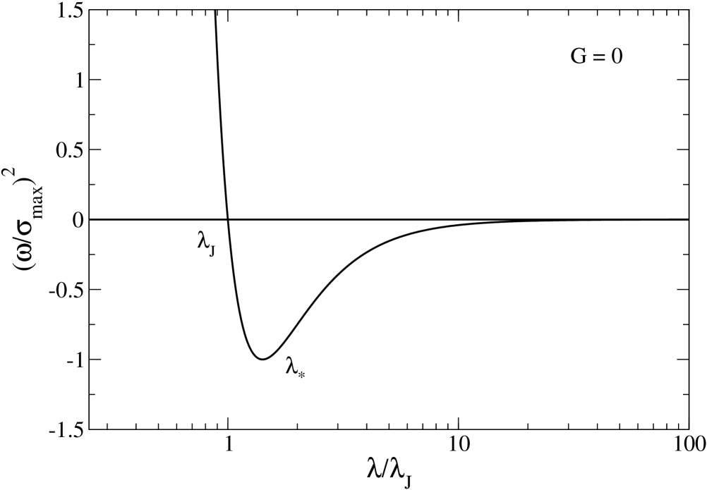
Figure 20: Growth rate $\sigma=(-\omega^{2})^{1/2}$ of the perturbations for nonrelativistic self-attracting bosons ($a_{s}<0$) in the nongravitational limit ($G=0$) as a function of the wavelength $\lambda$ (see Eq. (83)). The growth rate is normalized by the maximum growth rate $\sigma_{\rm max}$ and the wavelength by the Jeans length $\lambda_{J}$. The instability is relatively peaked about the most unstable wavelength $\lambda_{*}=\sqrt{2}\lambda_{J}$. Therefore, structures can form with a typical size $\sim\lambda_{*}$.

Remark: At the present epoch, we find that $\alpha=1.58\times 10^{-4}$ (corresponding to $\rho_{0}=2.25\times 10^{-24}\,{\rm g/m^{3}}\ll\rho_{a}=9.02\times 10^{-17}\,{\rm g}/{\rm m}^{3}$) and $\nu=6.53\times 10^{-16}$ (corresponding to $\rho_{i}=1.15\times 10^{-9}\,{\rm g}/{\rm m}^{3}\gg\rho_{0}=2.25\times 10^{-24}\,{\rm g}/{\rm m}^{3}$), so that we are in the noninteracting and nonrelativistic limit of Sec. VIII.3.

IX Jeans type instability of fermionic dark matter

In the preceding sections, we have considered the Jeans instability of a completely condensed self-gravitating relativistic boson gas at $T=0$. In this section, to make a comparison, we consider the same problem for a completely degenerate self-gravitating relativistic fermion gas at $T=0$. In the case of BECs, gravitational collapse is prevented by the Heisenberg uncertainty principle or by the self-repulsion of the bosons (when $a_{s}>0$). In the case of fermions, gravitational collapse is prevented by the Pauli exclusion principle (like in the case of white dwarfs and neutron stars).

IX.1 The ultrarelativistic limit

In the ultrarelativistic limit, a gas of fermions with spin $s=1/2$ has an equation of state chandrabook :

$$P=\frac{1}{8}\left(\frac{3}{\pi}\right)^{1/3}\frac{hc}{m^{4/3}}\rho^{4/3},$$ (156)

where $\rho=nm$ is the rest-mass density. This corresponds to a polytrope of index $n=3$. Expressed in terms of the energy density chandrabook :

$$\epsilon=\frac{3}{8}\left(\frac{3}{\pi}\right)^{1/3}\frac{hc}{m^{4/3}}\rho^{4/3},$$ (157)

we obtain

$$P=\frac{1}{3}\epsilon.$$ (158)

Since the equation of state of ultrarelativistic fermions is the same as radiation our results will be identical to those obtained in Sec. VII.3 for ultrarelativistic bosons.

Using the results of Appendix E, we find that the Jeans wavenumber and the Jeans length are given by

$$k_{J}^{2}=\frac{16\pi G\epsilon}{c^{4}},\qquad\lambda_{J}=2\pi\left(\frac{c^{4}}{16\pi G\epsilon}\right)^{1/2}.$$ (159)

Expressing the energy density in terms of the rest-mass density from Eq. (157), we obtain

$$\lambda_{J}=\frac{1}{\sqrt{3}}\left(\frac{\pi}{3}\right)^{1/6}\left(\frac{c^{3}}{G\hbar}\right)^{1/2}\left(\frac{m}{\rho}\right)^{2/3}.$$ (160)

Using Eq. (159), the Jeans mass (93) is given by

$$M_{J}=\frac{\pi^{5/2}}{48}\frac{c^{4}}{G^{3/2}\epsilon^{1/2}}.$$ (161)

It can also be written as

$$M_{J}=\frac{\pi^{2}}{24\sqrt{3}}\left(\frac{\pi}{3}\right)^{1/6}\left(\frac{c^{7}}{\hbar G^{3}}\right)^{1/2}\left(\frac{m}{\rho}\right)^{2/3}.$$ (162)

Eliminating the energy density between Eqs. (159) and (161), we get

$$M_{J}=\frac{\pi^{2}}{24}\frac{c^{2}\lambda_{J}}{G}.$$ (163)

This relation is similar to the mass-radius relation of a general relativistic star with a linear equation of state $P=\epsilon/3$ confined within a box aaq . In the present case, this agreement can be explained by the fact that the equation of state of an ultrarelativistic Fermi gas is $P=\epsilon/3$ (like radiation). Comparing Eq. (96) with $q=1/3$ and Eq. (163), we obtain

$$\frac{M_{J}}{\lambda_{J}/2}=3.84\frac{M}{R}.$$ (164)

Introducing the scales $\lambda_{F}$, $M_{F}$, $\rho_{F}$ (see Appendix D.7) and the relativistic parameter $\mu=(\rho/\rho_{F})^{2/3}$ appropriate to fermions (see Appendix F.6.1), we obtain

$$\frac{\lambda_{J}}{\lambda_{F}}=\frac{1}{\sqrt{3}}\left(\frac{\pi}{3}\right)^{1/6}\frac{1}{\mu},\qquad\frac{M_{J}}{M_{F}}=\frac{\pi^{2}}{24\sqrt{3}}\left(\frac{\pi}{3}\right)^{1/6}\frac{1}{\mu},$$ (165)

$$\frac{M_{J}}{M_{F}}=\frac{\pi^{2}}{24}\frac{\lambda_{J}}{\lambda_{F}}.$$ (166)

Since $\mu\gg 1$ (i.e. $\rho\gg\rho_{F}$) in the ultrarelativistic limit, we find that $\lambda_{J}\ll\lambda_{F}$ and $M_{J}\ll M_{F}$.

Introducing the Hubble scales $\lambda_{H}$ and $M_{H}$ (see Appendix D.1), we obtain

$$\frac{\lambda_{J}}{\lambda_{H}}=\frac{2\pi}{\sqrt{6}},\qquad\frac{M_{J}}{M_{H}}=\frac{1}{8}\left(\frac{2}{3}\right)^{3/2}\pi^{3}.$$ (167)

We note that $\lambda_{J}\sim\lambda_{H}$ and $M_{J}\sim M_{H}$. Since the Jeans length is of the order of the Hubble length (horizon), there is no Jeans instability. Therefore, large-scale structures cannot form in the ultrarelativistic limit.

Remark: The previous results are based on a general relativistic treatment. If we use a Newtonian treatment, we find from Eqs. (2) and (156) that the Jeans length is given by

$$\lambda_{J}=\sqrt{\frac{\pi}{6}}\left(\frac{3}{\pi}\right)^{1/6}\left(\frac{hc}{G}\right)^{1/2}\frac{1}{m^{2/3}\rho^{1/3}}.$$ (168)

The corresponding Jeans mass, defined by Eq. (125), is

$$M_{J}=\frac{\pi^{2}}{6\sqrt{72}}\left(\frac{hc}{G}\right)^{3/2}\frac{1}{m^{2}}.$$ (169)

This relation is similar to the Chandrasekhar mass of Newtonian ultrarelativistic self-gravitating fermions

$$M=0.376\left(\frac{hc}{G}\right)^{3/2}\frac{1}{m^{2}}.$$ (170)

Comparing Eqs. (169) and (170), we find that

$$M_{J}=0.516M.$$ (171)

Introducing the scales $\lambda_{F}$, $M_{F}$, $\rho_{F}$ (see Appendix D.7) and the relativistic parameter $\mu=(\rho/\rho_{F})^{2/3}$ appropriate to fermions (see Appendix F.6.2), we get

$$\frac{\lambda_{J}}{\lambda_{F}}=\frac{\pi^{5/6}}{3^{1/3}\sqrt{\mu}},\qquad\frac{M_{J}}{M_{F}}=\frac{\pi^{7/2}}{18}.$$ (172)

Since $\mu\gg 1$ (i.e. $\rho\gg\rho_{F}$) in the ultrarelativistic limit, we find that $\lambda_{J}\ll\lambda_{F}$ and $M_{J}\sim M_{F}$. We shall not discuss the Hubble length here because the Newtonian treatment is not valid in the ultrarelativistic limit.

IX.2 The nonrelativistic limit

In the nonrelativistic limit, a gas of fermions with spin $s=1/2$ has an equation of state chandrabook :

$$P=\frac{1}{20}\left(\frac{3}{\pi}\right)^{2/3}\frac{h^{2}}{m^{8/3}}\rho^{5/3},$$ (173)

where $\rho=nm$ is the rest-mass density. This corresponds to a polytrope of index $n=3/2$. Using Eq. (2), the Jeans length is given by

$$\lambda_{J}=\frac{1}{2}\left(\frac{\pi}{3}\right)^{1/6}\frac{h}{G^{1/2}m^{4/3}\rho^{1/6}}.$$ (174)

The associated Jeans mass, defined by Eq. (125), is

$$M_{J}=\frac{1}{16}\left(\frac{\pi}{3}\right)^{3/2}\frac{h^{3}\rho^{1/2}}{G^{3/2}m^{4}}.$$ (175)

Introducing relevant scales, we get

$$\frac{\lambda_{J}}{\rm pc}=1.94\times 10^{3}\,\left(\frac{{\rm eV}/c^{2}}{m}\right)^{4/3}\left(\frac{\rm g/m^{3}}{\rho}\right)^{1/6},$$ (176)

$$\frac{M_{J}}{M_{\odot}}=5.63\times 10^{25}\,\left(\frac{{\rm eV}/c^{2}}{m}\right)^{4}\left(\frac{\rho}{\rm g/m^{3}}\right)^{1/2}.$$ (177)

In the matter era, using Eq. (120), we find that the Jeans length increases as $a^{1/2}$ and the Jeans mass decreases as $a^{-3/2}$. Eliminating the density between Eqs. (174) and (175), we obtain

$$M_{J}\lambda_{J}^{3}=\frac{\pi^{2}}{1152}\frac{h^{6}}{G^{3}m^{8}}.$$ (178)

This relation is similar to the mass-radius relation of nonrelativistic self-gravitating fermions

$$MR^{3}=1.49\times 10^{-3}\frac{h^{6}}{G^{3}m^{8}}.$$ (179)

Comparing Eqs. (178) and (179), we find that

$$M_{J}\left(\frac{\lambda_{J}}{2}\right)^{3}=0.719MR^{3}.$$ (180)

Introducing the scales $\lambda_{F}$, $M_{F}$, $\rho_{F}$ (see Appendix D.7) and the relativistic parameter $\mu=(\rho/\rho_{F})^{2/3}$ appropriate to fermions (see Appendix F.6.2), we get

$$\frac{\lambda_{J}}{\lambda_{F}}=\pi\left(\frac{\pi}{3}\right)^{1/6}\frac{1}{\mu^{1/4}},\qquad\frac{M_{J}}{M_{F}}=\frac{\pi^{3}}{2}\left(\frac{\pi}{3}\right)^{3/2}\mu^{3/4},$$ (181)

$$\frac{M_{J}}{M_{F}}=\frac{\pi^{8}}{18}\left(\frac{\lambda_{F}}{\lambda_{J}}\right)^{3}.$$ (182)

Since $\mu\ll 1$ (i.e. $\rho\ll\rho_{F}$) in the nonrelativistic limit, we find that $\lambda_{J}\gg\lambda_{F}$ and $M_{J}\ll M_{F}$. We note that the relativistic parameter $\mu$ can be expressed in terms of the Hubble constant as $\mu=(3/8\pi)^{2/3}(H^{2}\hbar^{3}/Gm^{4}c^{3})^{2/3}$.

Introducing the Hubble scales $\lambda_{H}$ and $M_{H}$ (see Appendix D.1), we obtain

$$\frac{\lambda_{J}}{\lambda_{H}}=2\sqrt{2}\pi\left(\frac{\pi}{3}\right)^{2/3}\mu^{1/2},\qquad\frac{M_{J}}{M_{H}}=\frac{2\sqrt{2}}{9}\pi^{5}\mu^{3/2}.$$ (183)

Since $\mu\ll 1$ in the nonrelativistic limit, we find that $\lambda_{J}\ll\lambda_{H}$ and $M_{J}\ll M_{H}$. Therefore, large-scale structures can form in the nonrelativistic regime by Jeans instability since the Jeans length is much smaller than the horizon.

Let us consider a fermionic particle, like a sterile neutrino, able to form giant fermion balls with the mass and size of DM halos. To determine its mass $m$, we assume that the most compact DM halos observed in the Universe, namely dwarf spheroidals (dSphs) like Fornax ($R\sim 1\,{\rm kpc}$, $M\sim 10^{8}\,M_{\odot}$, $\overline{\rho}\sim 10^{-18}\,{\rm g/m^{3}}$), are completely degenerate, corresponding to the ground state of the self-gravitating Fermi gas. The mass-radius relation (179) then gives a fermion mass $m=170\,{\rm eV}/c^{2}$ (see Appendix D of suarezchavanis3 ). We note that, inversely, the knowledge of the DM particle mass $m$ does not determine $M$ and $R$ individually, but only their product $MR^{3}$. The individual determination of $M$ and $R$ depends on the epoch (time, scale factor, or redshift) and can be obtained from the Jeans study. Let us apply this study at the epoch of radiation-matter equality. For a fermion mass $m=170\,{\rm eV}/c^{2}$, we find that the dimensionless relativistic parameter defined by Eq. (256) is $\mu=5.89\times 10^{-7}$. The smallness of this value shows that we are in the nonrelativistic limit (the transition between the ultrarelativistic limit and the nonrelativistic limit takes place at $\rho_{F}=1.94\times 10^{-4}\,{\rm g}/{\rm m}^{3}\gg\rho_{\rm eq}=8.77\times 10^{-14}\,{\rm g}/{\rm m}^{3}$). To evaluate the Jeans length and the Jeans mass at the epoch of radiation-matter equality we use Eqs. (174) and (175) and obtain $\lambda_{J}=309\,{\rm pc}$ and $M_{J}=2.00\times 10^{10}\,M_{\odot}$. In comparison, $\lambda_{H}=4.40\times 10^{4}\,{\rm pc}$, $M_{H}=4.59\times 10^{17}\,M_{\odot}$, $\lambda_{F}=2.70\,{\rm pc}$ and $M_{F}=5.64\times 10^{13}\,M_{\odot}$. The relativistic corrections are negligible since $\mu\ll 1$. We also note that the comoving Jeans length is, at the epoch of radiation-matter equality, equal to $\lambda_{J}^{c}=1.05\,{\rm Mpc}$. The dicussion is essentially the same as for bosons (see Secs. VIII.3.2 and VIII.4.2). Indeed, at a qualitative level, fermions and bosons behave relatively similarly, as noted in kingclassique ; kingfermionic . The main differences are quantitative: (i) the mass of the fermionic DM particle is much larger than its bosonic counterpart; (ii) the solitonic/BEC core in bosonic DM halos is replaced by a fermion ball in fermionic DM halos.

Remark: If we compute the Jeans length and the Jeans mass at the present epoch, we find $\mu=5.13\times 10^{-14}$, $\lambda_{J}=18.0\,{\rm kpc}$, $M_{J}=1.01\times 10^{5}\,M_{\odot}$. In comparison $\lambda_{H}=8.69\times 10^{6}\,{\rm kpc}$, $M_{H}=9.06\times 10^{22}\,M_{\odot}$, $\lambda_{F}=2.70\,{\rm pc}$ and $M_{F}=5.64\times 10^{13}\,M_{\odot}$.

X Conclusion

The main idea when considering the formation of the large-scale structures of the Universe is that of gravitational instability. Usually, it is assumed that there exist small primordial perturbations which gradually increase in amplitude to form the structures that are being observed at present at the scale of galaxies and galaxy clusters. An overdense region is expected to attract material from its surroundings and become even denser. The denser they become the more they accrete, ending in an instability which can finally cause the collapse of a fluctuation to a gravitationally bound object. The knowledge of the Jeans length $\lambda_{J}$ gives an estimate of the minimum size of the objects that can form by gravitational instability.

In this paper, we have studied in detail the Jeans instability of a complex self-interacting SF in general relativity. This study is rather academic since the expansion of the Universe is neglected but it remains fundamentally interesting and important. In particular, it allows us to isolate characteristic length, mass and density scales that play a crucial role in any treatment of perturbations and structure formation in cosmology. This study was initiated in the seminal work of Khlopov et al. khlopov but our study goes beyond certain approximations made by these authors and completes their work.

Our approach is rather original with respect to other works on SFs. Indeed, instead of solving the field equations as usually done, we have used a hydrodynamic representation of the KGE equations introduced in our previous work suarezchavanis1 . We stress that for a complex SF this hydrodynamic representation is exact in the sense that the hydrodynamic equations are equivalent to the KGE equations. This hydrodynamic approach allows us to treat the problem of structure formation on the same footing as the original Jeans study for a classical self-gravitating collisional gas jeans1902 . Our approach is, however, much more general since it includes quantum mechanics ($\hbar$) and relativity ($c$) in addition to self-gravity ($G$) and pressure due to the self-interaction ($a_{s}$).

In this paper, we have studied the general dispersion relation $\omega(k)$ of a relativistic and quantum fluid obtained in suarezchavanis1 and deduced from it the Jeans length $\lambda_{J}$, the most unstable wavelength $\lambda_{*}$, and the maximum growth rate $\sigma_{\rm max}$. We have determined how the Jeans length and the Jeans mass vary as a function of the density of the Universe (the density of the Universe, as well as the scale factor or the redshift, can be considered as a measure of time in the cosmic history of the SF). This allowed us to analyze the cosmological evolution of the Jeans scales. We have stressed the analogy, previously noticed in prd1 , between the Jeans mass-radius relation $M_{J}(\lambda_{J})$ in the linear regime of structure formation and the mass-radius relation $M(R)$ of boson stars and dark matter halos in the nonlinear regime of structure formation (this analogy will be further developed in a future work prep ). We have considered different limits (ultrarelativistic, nonrelativistic, noninteracting, TF, nongravitational) and we have given precise conditions of validity of these different limits in terms of dimensionless parameters depending on the characteristics of the SF (mass and scattering length) and on the density of the Universe. We have given the numerical values of the Jeans mass and Jeans length at the epoch of radiation-matter equality (and at the current epoch for comparison) for different types of bosonic particles (QCD axions, ultralight axions, self-interacting bosons…). Our study therefore refines and completes previous works on the subject.

We have shown that structure formation is impossible in the early Universe (stiff matter era and radiationlike era) because the Jeans length is always larger than the Hubble length (horizon). This corresponds to the ultrarelativistic limit of our formalism. There is, however, an exception when the SF has an attractive self-interaction. In that case, the instability is caused by the self-interaction, not by the self-gravity which is usually negligible. If the boson has a mass $m=10^{-4}\,{\rm eV}/c^{2}$ and a negative scattering length $a_{s}=-5.8\times 10^{-53}\,{\rm m}$ (similarly to the QCD axion), one can form small objects with a size $\lambda_{J}=1.07\,{\rm cm}$ and a mass $M_{J}=3.41\times 10^{-21}M_{\odot}$. These objects, corresponding to a complex SF with an attractive self-interaction, are the counterparts of the axitons hr ; kt ; kt2 with size $R_{\rm axiton}\sim 10^{9}\,{\rm m}$ and mass $M_{\rm axiton}\sim 10^{-12}\,M_{\odot}$ corresponding to a real SF with an attractive self-interaction (QCD axion). On the other hand, if the boson has an ultrasmall mass $m=2.19\times 10^{-22}\,{\rm eV}/c^{2}$ and a negative scattering length $a_{s}=-1.11\times 10^{-62}\,{\rm fm}$, one can form big objects (protogalaxies) with a size $\lambda_{J}=0.159\,{\rm pc}$ and a mass $M_{J}=1.78\times 10^{4}\,M_{\odot}$. These objects could be the germs in the process of galaxy formation. Since these germs appear in the ultrarelativistic regime, the resulting galaxies would be much older than what is usually believed, possibly in agreement with certain recent cosmological observations where large-scale structures are observed at high redshifts nature .

We have shown that structure formation can take place in the matter era due to gravitational attraction. This corresponds to the nonrelativistic limit of our formalism. We have obtained the following results. For QCD axions with a mass $m=10^{-4}\,{\rm eV}/c^{2}$ and a scattering length $a_{s}=-5.8\times 10^{-53}\,{\rm m}$ we have shown that the self-interaction can be neglected in the matter era. The Jeans length is of the order of the Solar System size and the Jeans mass is of the order of the asteroid mass. Therefore, at the galactic level, QCD axions behave essentially as CDM and cannot solve the CDM crisis. They can form mini-MACHOSs (mini axion stars) that could be the constituents of DM halos, but they cannot form DM halos themselves. By contrast, for noninteracting ULAs with $m=2.92\times 10^{-22}\,{\rm eV/c^{2}}$, for self-repulsive bosons with a ratio $a_{s}/m^{3}=3.28\times 10^{3}\,{\rm fm}/({\rm eV/c^{2}})^{3}$ that are in the TF regime, and for ULAs with a mass $m=2.19\times 10^{-22}\,{\rm eV/c^{2}}$ and a negative scattering length $a_{s}\sim-1.11\times 10^{-62}\,{\rm fm}$ (corresponding to a ratio $|a_{s}|/m^{3}=1.06\times 10^{3}\,{\rm fm}/({\rm eV/c^{2}})^{3}$) that are in the nongravitational regime we find that the Jeans length and the Jeans mass are of the order of the galactic size. Therefore, they are good candidates to form DM halos. The study of the Jeans instability is not sufficient to discriminate these different particles but other considerations shapiro ; suarezchavanis3 suggest that axions must be self-interacting.

We have shown that, in the matter era, general relativistic effects become important at very large scales, of the order of the Hubble length $\lambda_{H}$, and tend to stabilize the system. Therefore, structure formation can take place for $\lambda_{J}\leq\lambda\leq\lambda_{H}$. Below the Jeans length there is no instability because gravity is too weak and above the Hubble length the growth rate decreases substantially because of general relativity. In between, the growth rate is almost constant, leading to a plateau $[10\lambda_{J},\lambda_{H}]$ where $\sigma\simeq\sigma_{\rm max}$. This implies that the optimal wavelength $\lambda_{*}$ is finite. By contrast, in the nonrelativistic model, the plateau $[10\lambda_{J},+\infty[$ extends to infinity and the optimal wavelength $\lambda_{*}\rightarrow+\infty$. Therefore, relativistic effects can solve some problems of the classical Jeans study, providing a maximum scale (of the order of the horizon) above which there is no gravitational instability anymore. Although these results have already been obtained in other contexts, it is interesting to recover them in a rigorous manner for a complex SF in a static background. In particular, our study extends the previous study of Khlopov et al. khlopov where these effects were neglected.

The SF model may have profound cosmological implications. DM is usually described by hydrodynamical equations without the quantum potential. In the context of CDM models with vanishing temperature and vanishing pressure, the usual Jeans analysis predicts that all scales are unstable. Consequently, the Jeans scale $\lambda_{J}$ is zero. This is the intrinsic reason why the CDM model generates cuspy dark matter halo profiles and an abundance of low mass halos. However, these cusps and satellites are not observed burkert ; firmani ; kauffmann . These problems (small-scale crisis of the CDM model) can be solved if the DM in the Universe is made up of a SF. In that case, the wave properties of the dark matter can stabilize gravitational collapse, providing halo cores and suppressing small-scale structures. Indeed, if DM is a SF, there exists a nonzero Jeans length. Stability below the Jeans scale is guaranteed by the Heisenberg uncertainty principle or by the pressure arising from the repulsive interaction of the bosons. This non-thermal quantum pressure stabilizes the system against gravitational collapse. For wavelengths smaller than the Jeans length, the evolution cannot bring the small perturbations in the early Universe to the nonlinear regime, and the inhomogeneities are erased (they remain oscillating modes). These modes are expected to induce a cutoff in the mass power spectrum for the distribution of galaxies in the Universe. For wavelengths larger than the Jeans length, the SF follows the evolution of the standard CDM scenario. Therefore, the SF and the CDM model differ at small scales while they are indistinguishable at large scales. Cosmological simulations are required to determine the viability of the SF/BECDM model.

The study in this work was motivated by the proposal that DM could be made out of SFs. Still, the nature of DM remains unknown. There exist other theories according to which DM could be made of massive neutrinos (see, e.g., vega ; ruffini ; kingclassique ; kingfermionic and references therein). In these theories, gravitational collapse is prevented by the Pauli exclusion principle for fermions. We have made a comparison between the Jeans problem for fermions and bosons. Qualitatively, the two types of particles behave similarly and are able to account for the observations. The main differences between fermionic and bosonic DM are quantitative. In particular, the mass of the fermionic DM particle ($m=170\,{\rm eV}/c^{2}$) is much larger than the mass of the bosonic DM particle ($m=2.92\times 10^{-22}\,{\rm eV}/c^{2}<m<1.10\times 10^{-3}\,{\rm eV/c^{2}}$) because the quantum pressure is due to the Pauli exclusion principle instead of the Heisenberg uncertainty principle or the repulsive scattering of the bosons (see Appendix D of suarezchavanis3 ). On the other hand, the gravitational collapse of self-gravitating fermions leads to DM halos with a core-halo structure made of a “fermion ball” surrounded by an isothermal (or NFW) atmosphere vega ; ruffini ; kingclassique ; kingfermionic while the gravitational collapse of self-gravitating BECs leads to DM halos with a core-halo structure made of a solitonic/BEC core surrounded by an isothermal (or NFW) atmosphere ch2 ; ch3 ; epjplusarejouter . Since it does not seem possible at the present stage to make a clear distinction (from observations) between a fermionic core and a bosonic core, it is not easy to determine whether DM is made of bosons or fermions.

Appendix A Dimensionless variables

In order to simplify the calculations and make the figures, it is convenient to introduce dimensionless variables. Different choices are possible depending on the parameters that we fix to construct the reference scales. We present below the two normalizations used in this paper, but other normalizations are possible.

A.1 First normalization: $G$ and $\hbar$ fixed

We introduce the reference pulsation and the reference wavenumber

$$\omega_{0}=\sqrt{4\pi G\rho},\qquad k_{0}=\left(\frac{16\pi G\rho m^{2}}{\hbar^{2}}\right)^{1/4}.$$ (184)

The pulsation $\omega_{0}$ coincides with the inverse dynamical time and the wavenumber $k_{0}$ coincides with the quantum Jeans wavenumber (37) in the nonrelativistic limit. We define the dimensionless variables

$$\Omega=\frac{\omega}{\omega_{0}},\qquad\kappa=\frac{k}{k_{0}},$$ (185)

$$\alpha=\left(\frac{m^{2}c_{s}^{4}}{4\pi G\rho\hbar^{2}}\right)^{1/2},\qquad\chi=\left(\frac{4\pi G\rho\hbar^{2}}{m^{2}c^{4}}\right)^{1/2}.$$ (186)

We note that $\alpha\chi=c_{s}^{2}/c^{2}$. We also note that $\chi=\omega_{0}/\omega_{C}$, where $\omega_{C}=c/\lambda_{C}=mc^{2}/\hbar$ is the Compton pulsation ($\lambda_{C}=\hbar/mc$ is the Compton wavelength). In this normalization, $G$ and $\hbar$ are used to construct the reference scales $\omega_{0}$ and $k_{0}$, so they are assumed to be “fixed”. Then, the parameter $\alpha\propto c_{s}^{2}$ measures the speed of sound (self-interaction) and the parameter $\chi\propto 1/c^{2}$ measures the importance of relativistic effects. The noninteracting limit ($c_{s}\rightarrow 0$) corresponds to $\alpha\rightarrow 0$ and the nonrelativistic limit ($c\rightarrow+\infty$) corresponds to $\chi\rightarrow 0$. For a quartic SF potential of the form of Eq. (13), using the expression of the speed of sound given by Eq. (21), we can write the parameter $\alpha$ as

$$\alpha=\left(\frac{4\pi\rho\hbar^{2}a_{s}^{2}}{Gm^{4}}\right)^{1/2}.$$ (187)

Remark: Using this normalization amounts to taking $4\pi G=\rho=2m=\hbar=1$, $\alpha=c_{s}^{2}/2$ and $\chi=2/c^{2}$ in the original equations.

A.2 Second normalization: $G$ and $c_{s}$ fixed

We introduce the reference pulsation and the reference wavenumber

$$\omega_{0}=\sqrt{4\pi G\rho},\qquad k_{0}=\left(\frac{4\pi G\rho}{c_{s}^{2}}\right)^{1/2}.$$ (188)

The pulsation $\omega_{0}$ coincides with the inverse dynamical time and the wavenumber $k_{0}$ coincides with the classical Jeans wavenumber (40) in the nonrelativistic limit. We define the dimensionless variables

$$\Omega=\frac{\omega}{\omega_{0}},\qquad\kappa=\frac{k}{k_{0}},$$ (189)

$$\nu=\frac{c_{s}^{2}}{c^{2}},\qquad\epsilon=\frac{1}{\alpha}=\left(\frac{4\pi G\rho\hbar^{2}}{m^{2}c_{s}^{4}}\right)^{1/2}.$$ (190)

In this normalization, $G$ and $c_{s}$ are used to construct the reference scales $\omega_{0}$ and $k_{0}$, so they are assumed to be “fixed”. Then, the parameter $\nu\propto 1/c^{2}$ measures the importance of relativistic effects and the parameter $\epsilon\propto\hbar$ measures the importance of quantum effects. The nonrelativistic limit ($c\rightarrow+\infty$) corresponds to $\nu\rightarrow 0$ and the TF limit ($\hbar\rightarrow 0$) corresponds to $\epsilon\rightarrow 0$. For a quartic SF potential of the form of Eq. (13), using the expression of the speed of sound given by Eq. (21), we can write the parameter $\nu$ as

$$\nu=\frac{4\pi|a_{s}|\hbar^{2}\rho}{m^{3}c^{2}}.$$ (191)

Remark: Using this normalisation amounts to taking $4\pi G=\rho=c_{s}=m=1$, $\nu=1/c^{2}$ and $\epsilon=1/\alpha=\hbar$ in the original equations.

Appendix B Optimal wavenumber and maximum growth rate in the noninteracting limit

In this Appendix, we determine the most unstable wavenumber $k_{*}$ and the maximum growth rate $\sigma_{\rm max}$ in the noninteracting limit ($a_{s}=0$) for the simplified and exact relativistic models. We give their asymptotic behaviors in the nonrelativistic ($c\rightarrow+\infty$) and ultrarelativistic ($c\rightarrow 0$) limits.

B.1 Simplified relativistic model

Using the normalization of Appendix A.1, the dispersion relation of Eq. (49) takes the form

$$\frac{1}{4}\chi^{2}\Omega^{4}-(1+\chi\kappa^{2})\Omega^{2}+\kappa^{4}-1=0.$$ (192)

Its solutions are given by

$$\Omega^{2}_{\pm}(\kappa)=\frac{2}{\chi^{2}}\left[1+\chi\kappa^{2}\pm(1+2\chi\kappa^{2}+\chi^{2})^{1/2}\right].$$ (193)

The functions $\Omega^{2}_{\pm}(\kappa)$ are plotted in Figs. 3 and 4.

We first consider the branch (+). The minimum pulsation, corresponding to $\kappa_{*}=0$, is given by $(\Omega_{+})_{\rm min}=(\Omega_{+}^{2}(0))^{1/2}$ with

$$\Omega_{+}^{2}(0)=\frac{2}{\chi^{2}}\left(1+\sqrt{1+\chi^{2}}\right).$$ (194)

This function is plotted in Fig. 8. For $\chi\rightarrow 0$ (nonrelativistic limit):

$$\Omega_{+}^{2}(0)\sim\frac{4}{\chi^{2}}.$$ (195)

For $\chi\rightarrow+\infty$ (ultrarelativistic limit):

$$\Omega_{+}^{2}(0)\sim\frac{2}{\chi}.$$ (196)

We now consider the branch (-). The Jeans wavenumber is given by

$$\kappa_{J}^{2}=1.$$ (197)

The maximum growth rate, corresponding to $\kappa_{*}=0$, is given by $\Sigma_{\rm max}=(-\Omega_{-}^{2}(0))^{1/2}$ with

$$\Omega_{-}^{2}(0)=\frac{2}{\chi^{2}}\left(1-\sqrt{1+\chi^{2}}\right).$$ (198)

This function is plotted in Fig. 11. For $\chi\rightarrow 0$ (nonrelativistic limit):

$$\Omega_{-}^{2}(0)\simeq-1+\frac{\chi^{2}}{4}.$$ (199)

For $\chi\rightarrow+\infty$ (ultrarelativistic limit):

$$\Omega_{-}^{2}(0)\sim-\frac{2}{\chi}.$$ (200)

B.2 Exact relativistic model

Using the normalization of Appendix A.1, the dispersion relation of Eq. (66) takes the form

$$\frac{1}{4}\chi^{2}\Omega^{4}-\left(\frac{1+\gamma}{3\gamma+1}\chi\kappa^{2}+1\right)\Omega^{2}$$

$$+\frac{1}{1+3\gamma}\left[(1-\gamma)\kappa^{4}-1\right]=0$$ (201)

with

$$\gamma=\frac{\chi}{2\kappa^{2}}.$$ (202)

The functions $\Omega^{2}_{\pm}(\kappa)$ are plotted in Figs. 6 and 7.

We first consider the branch (+). The minimum pulsation, corresponding to $\kappa=0$, is given by $(\Omega_{+})_{\rm min}=(\Omega_{+}^{2}(0))^{1/2}$ with

$$\Omega_{+}^{2}(0)=\frac{4}{\chi^{2}}.$$ (203)

This function is plotted in Fig. 8.

We now consider the branch (-). The Jeans wavenumber is

$$\kappa_{J}^{2}=\frac{1}{4}\left(\chi+\sqrt{16+\chi^{2}}\right).$$ (204)

This function is plotted in Fig. 9. For $\chi\rightarrow 0$ (nonrelativistic limit):

$$\kappa_{J}^{2}\rightarrow 1.$$ (205)

For $\chi\rightarrow+\infty$ (ultrarelativistic limit):

$$\kappa_{J}^{2}\sim\frac{\chi}{2}.$$ (206)

The wavenumber $\kappa_{*}$ corresponding to the maximum growth rate is obtained from the condition $(\Omega^{2})^{\prime}(\kappa_{*})=0$ where $\Omega^{2}(\kappa)$ is the solution of the second degree equation (201). Instead of solving Eq. (201) for $\Omega^{2}(\kappa)$ and taking the derivative of this function with respect to $\kappa$, we proceed as follows. We multiply Eq. (201) by $2\kappa^{2}(3\gamma+1)$, differentiate the resulting expression with respect to $\kappa$, and cancel the terms where $(\Omega^{2})^{\prime}(\kappa)=0$ appear. In this way we obtain

$$\chi^{2}\Omega^{4}-2\left(4\chi\kappa^{2}+\chi^{2}+2\right)\Omega^{2}+4\left(3\kappa^{4}-\chi\kappa^{2}-1\right)=0.$$ (207)

The most unstable wavenumber $\kappa_{*}$ and the corresponding maximum growth rate $\Sigma_{\rm max}=(-\Omega^{2}(\kappa_{*}))^{1/2}$ are then determined by Eqs. (201) and (207). The functions $\kappa_{*}(\chi)$ and $\Sigma_{\rm max}(\chi)$ are plotted in Figs. 10 and 11. Their asymptotic behaviors for small and large $\chi$ can be determined analytically.

For $\chi\rightarrow 0$ (nonrelativistic limit):

$$\kappa_{*}\sim A\,\chi^{1/6},$$ (208)

$$\Omega^{2}(\kappa_{*})\simeq-1+B\,\chi^{2/3},$$ (209)

where the coefficients $A$ and $B$ are determined by the algebraic equations

$$-B + \frac{3}{2A^{2}}+A^{4}=0,$$

$$-4B + 12A^{4}=0.$$ (210)

We obtain $A=0.953184...$ and $B=2.47645...$.

For $\chi\rightarrow\infty$ (ultrarelativistic limit):

$$\kappa_{*}\simeq\chi^{1/2}\left(C+\frac{D}{\chi^{2}}\right),$$ (211)

$$\Omega^{2}_{-}(\kappa_{*})\simeq A-\frac{B}{\chi^{2}},$$ (212)

where the coefficients $A$, $B$, $C$ and $D$ are determined by the algebraic equations

$$3A^{2} - 4AC^{2}+2A^{2}C^{2}-4C^{4}-8AC^{4}+8C^{6}=0,$$

$$-2A + A^{2}-4C^{2}-8AC^{2}+12C^{4}=0,$$

$$-\frac{AB}{2} + \frac{BC^{2}(1+2C^{2})}{3+2C^{2}}$$

$$+ \frac{2C^{2}(-3-2C^{2}-6CD+16C^{3}D+8C^{5}D)}{(3+2C^{2})^{2}}$$

$$- A\left[1+\frac{2(3CD+12C^{3}D+4C^{5}D)}{(3+2C^{2})^{2}}\right]=0,$$

$$-4 - 4A+2B-2AB+8BC^{2}-8CD-16ACD$$ (213)

$$+ 48C^{3}D=0.$$

We obtain $A=-0.0717968...$, $B=0.464102...$, $C=0.481717...$ and $D=0.898895...$.

The function $-\Omega^{2}(\kappa_{*})[\chi]$ starts from $1$ at $\chi=0$, decreases and tends to $0.0717968...$ as $\chi\rightarrow+\infty$.

Appendix C Optimal wavenumber and maximum growth rate in the TF case

In this Appendix, we determine the most unstable wavenumber $k_{*}$ and the maximum growth rate $\sigma_{\rm max}$ in the TF limit ($\hbar\rightarrow 0$) for the simplified and exact relativistic models. We give their asymptotic behaviors in the nonrelativistic ($c\rightarrow+\infty$) and ultrarelativistic ($c\rightarrow 0$) limits.

C.1 Simplified relativistic model

Using the normalization of Appendix A.2, the dispersion relation of Eq. (54) takes the form

$$\Omega^{2}=\frac{\kappa^{2}-1-2\nu}{1+3\nu}.$$ (214)

This function is plotted in Fig. 5. The Jeans wavenumber is given by

$$\kappa_{J}^{2}=1+2\nu.$$ (215)

This function is plotted in Fig. 13. For $\nu\rightarrow 0$ (nonrelativistic limit):

$$\kappa_{J}^{2}\rightarrow 1.$$ (216)

For $\nu\rightarrow+\infty$ (ultrarelativistic limit):

$$\kappa_{J}^{2}\sim 2\nu.$$ (217)

The maximum growth rate, corresponding to $\kappa=0$, is given by $\Sigma_{\rm max}=(-\Omega^{2}(0))^{1/2}$ with

$$\Omega^{2}(0)=-\frac{1+2\nu}{1+3\nu}.$$ (218)

This function is plotted in Fig. 15. For $\nu\rightarrow 0$ (nonrelativistic limit):

$$\Omega^{2}(0)\simeq-1+\nu.$$ (219)

For $\nu\rightarrow+\infty$ (ultrarelativistic limit):

$$\Omega^{2}(0)\simeq-\frac{2}{3}-\frac{1}{9\nu}.$$ (220)

C.2 Exact relativistic model

Using the normalization of Appendix A.2, the dispersion relation of Eq. (72) takes the form

$$\Omega^{2}=\frac{1}{\gamma}(1+2\nu)\frac{1}{1+3\gamma}\frac{\nu-(3\nu+1)\gamma}{1+3\nu}$$ (221)

with

$$\gamma=\frac{\nu}{\kappa^{2}}(1+2\nu).$$ (222)

This function is plotted in Fig. 12. The Jeans wavenumber is

$$\kappa_{J}^{2}=(1+2\nu)(1+3\nu).$$ (223)

This function is plotted in Fig. 13. For $\nu\rightarrow 0$ (nonrelativistic limit):

$$\kappa_{J}^{2}\rightarrow 1.$$ (224)

For $\nu\rightarrow+\infty$ (ultrarelativistic limit):

$$\kappa_{J}^{2}\sim 6\nu^{2}.$$ (225)

The maximum growth rate, obtained from the condition $(\Omega^{2})^{\prime}(\kappa_{*})=0$, corresponds to an optimal wavenumber $\kappa_{*}$ given by

$$\kappa_{*}^{2}=\frac{3(3\nu+1)(1+2\nu)\nu}{3\nu+\sqrt{3\nu(6\nu+1)}}.$$ (226)

An equivalent expression is

$$\kappa_{*}^{2}=3\nu(1+2\nu)\left(\sqrt{2+\frac{1}{3\nu}}-1\right).$$ (227)

The maximum growth rate $\Sigma_{\rm max}=\sqrt{-\Omega^{2}(\kappa_{*})}$ is then obtained by substituting Eq. (226) or Eq. (227) into Eq. (221). The functions $\kappa_{*}(\nu)$ and $\Sigma_{\rm max}(\nu)$ are plotted in Figs. 14 and 15.

For $\nu\rightarrow 0$ (nonrelativistic limit):

$$\kappa_{*}^{2}\sim\sqrt{3\nu},$$ (228)

$$\Omega^{2}(\kappa_{*})\simeq-1+2\sqrt{3\nu}+...$$ (229)

For $\nu\rightarrow+\infty$ (ultrarelativistic limit):

$$\kappa_{*}^{2}\sim\frac{6\nu^{2}}{1+\sqrt{2}},$$ (230)

$$\Omega^{2}(\kappa_{*})\sim 2(2\sqrt{2}-3)\nu.$$ (231)

The function $-\Omega^{2}(\kappa_{*})[\nu]$ starts from $1$ at $\nu=0$, decreases, reaches a minimum value $-\Omega^{2}(\kappa_{*})\simeq 0.438$ at $\nu\simeq 0.23$, increases and tends to $+\infty$ as $\nu\rightarrow+\infty$.

Appendix D Characteristic scales

In this Appendix, we introduce characteristic length, mass and density scales that play an important role in the astrophysical and cosmological applications considered in this paper (see Secs. VII-IX).

D.1 The Hubble scales

We introduce the Hubble length

$$\lambda_{H}=\frac{c}{H},$$ (232)

where $H=\dot{a}/a$ is the Hubble constant. The Hubble length represents the distance travelled by a photon with velocity $c$ during the Hubble time $t_{H}=1/H$ which gives the typical age of the Universe. Therefore, the Hubble length $\lambda_{H}=ct_{H}$ represents the typical size of the visible Universe (particle horizon). In a flat Universe, the Hubble constant is related to the energy density $\epsilon$ by the Friedmann equation weinbergbook :

$$H^{2}=\frac{8\pi G}{3c^{2}}\epsilon.$$ (233)

We introduce the Hubble mass $M_{H}=(4/3)\pi(\epsilon/c^{2})\lambda_{H}^{3}$. It represents the typical mass of the visible Universe. Using Eqs. (232) and (233), we get

$$M_{H}=\frac{c^{3}}{2GH}.$$ (234)

The Hubble length and the Hubble mass can also be written in terms of the energy density as

$$\lambda_{H}=\left(\frac{3c^{4}}{8\pi G\epsilon}\right)^{1/2},\qquad M_{H}=\left(\frac{3c^{8}}{32\pi G^{3}\epsilon}\right)^{1/2}.$$ (235)

They are connected to each other by the relation $\lambda_{H}=2GM_{H}/c^{2}$. This relation is similar to the Schwarzschild radius of a black hole

$$R_{S}=\frac{2GM}{c^{2}}.$$ (236)

Therefore, the Hubble length and the Hubble mass of the Universe display the same scaling as a Schwarzschild black hole (see Appendix F.5 of bectcoll ).

Remark: the current values of the Hubble scales are $H_{0}=2.18\times 10^{-18}\,{\rm s}^{-1}$, $t_{H}=1/H_{0}=14.5\,{\rm Gyrs}$, $\lambda_{H}=1.37\times 10^{26}\,{\rm m}$, $\epsilon_{0}/c^{2}=8.45\times 10^{-24}\,{\rm g/m^{3}}$, and $M_{H}=9.26\times 10^{55}\,{\rm g}$.

D.2 The scales associated with noninteracting relativistic self-gravitating BECs

We introduce the length and mass scales associated with noninteracting relativistic self-gravitating BECs:

$$\lambda_{C}=\frac{\hbar}{mc},\qquad M_{C}=\frac{\hbar c}{Gm}=\frac{M_{P}^{2}}{m},$$ (237)

where $M_{P}=(\hbar c/G)^{1/2}$ is the Planck mass. These scales appear in the works of Kaup kaup and Ruffini and Bonazzola rb on boson stars. $M_{C}$ is of the order of the maximum mass of a noninteracting relativistic self-gravitating BEC and $\lambda_{C}$, which coincides with the Compton length, is of the order of the corresponding (minimum) radius. They are connected to each other by the relativistic scaling $M_{C}=c^{2}\lambda_{C}/G$. We also introduce the density scale

$$\rho_{C}=\frac{m^{2}c^{4}}{8\pi G\hbar^{2}},$$ (238)

which is of the order of $M_{C}/\lambda_{C}^{3}$. We note that the relativistic parameter defined in Appendix A.1 can be written as

$$\chi=\left(\frac{\rho}{2\rho_{C}}\right)^{1/2}.$$ (239)

The mass-radius relation $M(R)$ (parametrized by the central energy density $\epsilon_{0}$) of noninteracting self-gravitating BECs in the context of general relativity is represented in Fig. 3 of seidel90 . In the nonrelativistic limit, the mass-radius relation is given by Eq. (130). The system becomes relativistic when its radius $R$ approaches the Schwarzschild radius $R_{S}$. This determines the maximum mass of a noninteracting boson star above which there is no equilibrium state. The spiral is made of unstable equilibrium states. Combining Eqs. (130) and (236) we obtain the scalings of Eqs. (237) and (238). By numerically solving the KGE equations, one gets the exact values $M_{\rm max}=0.633M_{C}$ and $R_{\rm min}=6.03\lambda_{C}$, where $R$ is the radius containing $95\%$ of the mass kaup ; rb .

D.3 The scales associated with self-repulsive relativistic self-gravitating BECs

We introduce the length and mass scales associated with relativistic self-gravitating BECs with a repulsive $|\varphi|^{4}$ self-interaction ($a_{s}>0$):

$$\lambda_{R}=\left(\frac{a_{s}\hbar^{2}}{Gm^{3}}\right)^{1/2},\qquad M_{R}=\left(\frac{a_{s}\hbar^{2}c^{4}}{G^{3}m^{3}}\right)^{1/2}.$$ (240)

Introducing the dimensionless self-interaction parameter (see Appendix B of suarezchavanis3 ):

$$\frac{\lambda}{8\pi}=\frac{a_{s}}{\lambda_{C}}=\frac{a_{s}mc}{\hbar},$$ (241)

they can be rewritten as

$$\lambda_{R}=\sqrt{\frac{\lambda}{8\pi}}\frac{M_{P}}{m}\lambda_{C},\qquad M_{R}=\sqrt{\frac{\lambda}{8\pi}}\frac{M_{P}^{3}}{m^{2}}.$$ (242)

These scales appear in the works of Colpi et al. colpi and Tkachev tkachev on boson stars and in the work of Chavanis and Harko chavharko on neutron stars with a superfluid core (BEC stars). $M_{R}$ is of the order of the maximum mass of a relativistic self-gravitating BEC in the TF limit and $\lambda_{R}$ is of the order of the corresponding (minimum) radius. They are connected to each other by the relativistic scaling $M_{R}=c^{2}\lambda_{R}/G$. We also introduce the density scale

$$\rho_{R}=\frac{m^{3}c^{2}}{6\pi a_{s}\hbar^{2}},$$ (243)

which is of the order of $M_{R}/\lambda_{R}^{3}$. We note that the relativistic parameter defined in Appendix A.2 can be written as

$$\nu=\frac{2\rho}{3\rho_{R}}.$$ (244)

The mass-radius relation $M(R)$ (parametrized by the central energy density $\epsilon_{0}$) of self-gravitating BECs with a repulsive self-interaction in the context of general relativity is represented in Fig. 9 of chavharko . In the nonrelativistic limit, the radius of the system is independent of its mass and given by Eq. (140). The system becomes relativistic when its radius $R$ approaches the Schwarzschild radius $R_{S}$. This determines the maximum mass of a self-repulsive boson star above which there is no equilibrium state. The spiral is made of unstable equilibrium states. Combining Eqs. (140) and (236) we obtain the scalings of Eqs. (240)-(243). By numerically solving the KGE equations colpi or the equivalent hydrodynamic equations chavharko , one gets the exact values $M_{\rm max}=0.307M_{R}$, $R_{\rm min}=1.92\lambda_{R}$ and $(\epsilon_{0})_{\rm max}=1.19\rho_{R}c^{2}$.

D.4 The scales associated with self-interacting nonrelativistic self-gravitating BECs

We introduce the length and mass scales associated with nonrelativistic self-gravitating BECs with a $|\psi|^{4}$ self-interaction:

$$\lambda_{a}=\left(\frac{|a_{s}|\hbar^{2}}{Gm^{3}}\right)^{1/2},\qquad M_{a}=\frac{\hbar}{\sqrt{Gm|a_{s}|}}.$$ (245)

These scales appear in the works of Chavanis prd1 ; prd2 ; bectcoll on self-gravitating BECs with attractive or repulsive self-interactions. For a repulsive self-interaction ($a_{s}>0$), they determine the transition between the noninteracting limit and the TF limit. For an attractive self-interaction ($a_{s}<0$), $M_{a}$ is of the order of the maximum mass of a self-gravitating BEC and $\lambda_{a}$ is of the order of the corresponding (minimum) radius. We also introduce the density scale

$$\rho_{a}=\frac{Gm^{4}}{4\pi\hbar^{2}a_{s}^{2}},$$ (246)

which is of the order of $M_{a}/\lambda_{a}^{3}$. We note that the self-interaction parameter defined in Appendix A.1 can be written as

$$\alpha=\left(\frac{\rho}{\rho_{a}}\right)^{1/2}.$$ (247)

The mass-radius relation $M(R)$ (parametrized by the central density $\rho_{0}$) of nonrelativistic self-gravitating BECs with a repulsive self-interaction is represented in Fig. 4 of prd2 . In the noninteracting limit, the mass-radius relation is given by Eq. (130). In the TF limit, the radius of the system is independent on its mass and given by Eq. (140). At the transition, combining Eqs. (130) and (140), we obtain the scalings of Eqs. (245) and (246).

The mass-radius relation $M(R)$ (parametrized by the central density $\rho_{0}$) of nonrelativistic self-gravitating BECs with an attractive self-interaction is represented in Fig. 6 of prd2 . In the noninteracting limit, the mass-radius relation is given by Eq. (130). In the nongravitational limit, the mass-radius relation is given by Eq. (151) but these equilibrium states are unstable. At the transition, combining Eqs. (130) and (151), we obtain the scalings of Eqs. (245) and (246). They determine the maximum mass of Newtonian self-attracting boson stars above which there is no equilibrium state. By numerically solving the GPP equations or the equivalent hydrodynamic equations prd2 , one gets the exact values $M_{\rm max}=1.012M_{a}$, $R_{\rm min}=5.5\lambda_{a}$ and $(\rho_{0})_{\rm max}=0.5\rho_{a}$.

D.5 The scales associated with self-attracting nongravitational BECs

We introduce the length and mass scales associated with nongravitational BECs with an attractive self-interaction ($a_{s}<0$):

$$\lambda_{i}=\frac{\hbar}{mc},\qquad M_{i}=\frac{\hbar}{|a_{s}|c}.$$ (248)

These scales appear in Sec. VII.4 of this paper. They correspond to the Jeans length and Jeans mass of a nongravitational BEC with attractive self-interaction in the ultrarelativistic limit. We note that $\lambda_{i}$ coincides with the Compton wavelength of the particle. To the best of our knowledge, the mass scale $M_{i}$ has not been introduced before. We also introduce the density scale

$$\rho_{i}=\frac{m^{3}c^{2}}{12\pi|a_{s}|\hbar^{2}},$$ (249)

which is of the order of $M_{i}/\lambda_{i}^{3}$. We note that the relativistic parameter defined in Appendix A.2 can be written as

$$\nu=\frac{\rho}{3\rho_{i}}.$$ (250)

Remark: these scales are embedded in the KG equation (16). Comparing the first and second terms, we obtain the length scale $\lambda_{i}=\hbar/mc$. Comparing the second and third terms, and using Eq. (19), we obtain the density scale $\rho_{i}={m^{3}c^{2}}/{12\pi|a_{s}|\hbar^{2}}$. From these two characteristic scales, we obtain the mass scale $M_{i}\sim\rho_{i}\lambda_{i}^{3}={\hbar}/{|a_{s}|c}$.

D.6 The effective Schwarzschild radius of a boson

Following Ref. suarezchavanis3 , we introduce the effective Schwarzschild radius of a boson

$$r_{S}=\frac{2Gm}{c^{2}}$$ (251)

and the self-interaction parameter

$$\sigma=\frac{3|a_{s}|c^{2}}{4Gm}=\frac{3|a_{s}|}{2r_{S}}.$$ (252)

We also introduce a density scale

$$\rho_{h}=\frac{|a_{s}|mc^{6}}{G^{2}\hbar^{2}}.$$ (253)

D.7 The scales associated with relativistic self-gravitating fermions

We introduce the length and mass scales associated with relativistic self-gravitating fermions:

$$\lambda_{F}=\left(\frac{\hbar^{3}}{Gc}\right)^{1/2}\frac{1}{m^{2}},\qquad M_{F}=\left(\frac{\hbar c}{G}\right)^{3/2}\frac{1}{m^{2}}=\frac{M_{P}^{3}}{m^{2}}.$$ (254)

These scales appear in the work of Chandrasekhar chandramax on white dwarf stars and in the work of Oppenheimer and Volkoff ov on neutron stars. $M_{F}$ is of the order of the maximum mass of a relativistic self-gravitating fermion star and $\lambda_{F}$ is of the order of the corresponding (minimum) radius. They are connected to each other by the relativistic scaling $M_{F}=c^{2}\lambda_{F}/G$. We also introduce the density scale

$$\rho_{F}=\frac{m^{4}c^{3}}{\hbar^{3}},$$ (255)

which is of the order of $M_{F}/\lambda_{F}^{3}$. We define the relativistic parameter for fermions by

$$\mu=\left(\frac{\rho\hbar^{3}}{m^{4}c^{3}}\right)^{2/3}=\left(\frac{\rho}{\rho_{F}}\right)^{2/3}.$$ (256)

The mass-radius relation $M(R)$ (parametrized by the central energy density $\epsilon_{0}$) of self-gravitating fermions in the context of general relativity is represented in Fig. 7 of ns . In the nonrelativistic limit, the mass-radius relation is given by Eq. (173). The system becomes relativistic when its radius $R$ approaches the Schwarzschild radius $R_{S}$. This determines the maximum mass of a fermion star above which there is no equilibrium state. The spiral is made of unstable equilibrium states. Combining Eqs. (173) and (236) we obtain the scalings of Eqs. (254) and (255). By numerically solving the equations of hydrostatic equilibrium in general relativity, one gets the exact values $M_{\rm max}=0.384M_{F}$, $R_{\rm min}=3.36\lambda_{F}$ and $(\epsilon_{0})_{\rm max}=2.33\times 10^{-2}\rho_{F}c^{2}$ ov ; ns .

Appendix E The general relativistic Jeans instability of a fluid

In this Appendix, we consider the Jeans instability of a self-gravitating fluid with an equation of state $P(\epsilon)$ in the framework of general relativity. We assume that this equation of state is valid for both homogeneous and inhomogeneous distributions. The exact Jeans wavenumber obtained from the Einstein equations slightly perturbed from a spatially homogeneous distribution is paddy :

$$k_{J}^{2}=\frac{4\pi G\epsilon}{c_{s}^{2}c^{2}}\left(1-6\frac{c_{s}^{2}}{c^{2}}+8w-3w^{2}\right),$$ (257)

where $c_{s}^{2}=P^{\prime}(\epsilon)c^{2}$ is the speed of sound in the homogeneous fluid and $w=P/\epsilon$ is the equation of state parameter.

For a nonrelativistic fluid ($c_{s}\ll c^{2}$, $w\ll 1$ and $\epsilon=\rho c^{2}$), Eq. (257) reduces to the standard Jeans formula of Eq. (2). For the equation of state of radiation $P=\epsilon/3$, we get

$$k_{J}^{2}=\frac{16\pi G\epsilon}{c^{4}}.$$ (258)

For the equation of state of stiff matter $P=\epsilon$, we obtain

$$k_{J}^{2}=0.$$ (259)

Since $\lambda_{J}\rightarrow+\infty$, there is no Jeans instability in a stiff fluid.

Appendix F Transition scales in cosmology

The Jeans mass-radius relations $M_{J}(\lambda_{J})$ (parametrized by the density of the universe $\rho$) in cosmology are similar to the mass-radius relations $M(R)$ (parametrized by the central density $\rho_{0}$) of boson stars and DM halos (see Appendix D). This similarity (noted in Sec. V of prd1 ) is not obvious since the first relations $M_{J}(\lambda_{J})$ are valid in the linear regime of structure formation (Jeans problem) while the second relations $M(R)$ are valid in the nonlinear regime of structure formation (DM halos $=$ equilibrium states). In the main text, we have given asymptotic expressions of $M_{J}(\lambda_{J})$ in different limits of physical interest. In this Appendix, we regroup these results in order to offer a clear relation between these different limits.

F.1 Transition scales in the noninteracting limit

We consider a SF in the noninteracting limit. The following results can be deduced from Eq. (71) using the scales of Appendix D.2.

The ultrarelativistic era (Sec. VII.2) corresponds to:

(i) $\chi\gg 1$.

(ii) $\rho\gg\rho_{C}$ (high densities/early Universe).

(iii) $\lambda_{J}\sim\lambda_{H}\ll\lambda_{C}$ and $M_{J}\sim M_{H}\ll M_{C}$.

The nonrelativistic era (Sec. VIII.3) corresponds to:

(i) $\chi\ll 1$.

(ii) $\rho\ll\rho_{C}$ (low densities/late Universe).

(iii) $\lambda_{C}\ll\lambda_{J}\ll\lambda_{H}$ and $M_{J}\ll M_{C}\ll M_{H}$.

Figure 21: Jeans mass-radius relation $M_{J}(\lambda_{J})$ parametrized by the density of the Universe $\rho$ in the noninteracting limit. The arrows indicate the cosmic evolution of the Universe from the ultrarelativistic (UR) regime at high densities [see Eq. (97)] to the nonrelativistic (NR) regime at low densities [see Eq. (132)]. This curve can be compared with the mass-radius relation $M(R)$ (parametrized by the central energy density $\epsilon_{0}$) of noninteracting self-gravitating BECs in the context of general relativity (see Fig. 3 of seidel90 ). The bullets correspond to ULAs and QCD axions at the epoch of radiation-matter equality considered in Secs. VIII.3.2 and VIII.3.3.

The Jeans mass-radius relation $M_{J}(\lambda_{J})$ presents a maximum $M_{C}$ at $\lambda_{C}$, corresponding to a density $\rho_{C}$ (see Fig. 21). The transition density $\rho_{C}$ where $\lambda_{J}\sim\lambda_{C}$ and $M_{J}\sim M_{C}$ separates the ultrarelativistic regime from the nonrelativistic regime. It corresponds to the density called $\rho_{v}(0)$ in suarezchavanis3 separating the stiff matter era (slow oscillation regime $\omega=mc^{2}/\hbar\ll H$) from the matterlike era (fast oscillation regime $\omega=mc^{2}/\hbar\gg H$). This is also the density below which the Jeans length is smaller than the Hubble length (horizon), allowing the formation of the large-scale structures of the universe.

F.2 Transition scales in the TF limit

We consider a SF with a repulsive self-interaction ($a_{s}>0$) in the TF limit. The following results can be deduced from Eq. (77) using the scales of Appendix D.3.

The ultrarelativistic era (Sec. VII.3) corresponds to:

(i) $\nu\gg 1$.

(ii) $\rho\gg\rho_{R}$ (high densities/early Universe).

(iii) $\lambda_{J}\sim\lambda_{H}\ll\lambda_{R}$ and $M_{J}\sim M_{H}\ll M_{R}$.

The nonrelativistic era (Sec. VIII.4) corresponds to:

(i) $\nu\ll 1$.

(ii) $\rho\ll\rho_{R}$ (low densities/late Universe).

(iii) $\lambda_{J}\sim\lambda_{R}\ll\lambda_{H}$ and $M_{J}\ll M_{R}\ll M_{H}$.

Figure 22: Jeans mass-radius relation $M_{J}(\lambda_{J})$ parametrized by the density of the Universe $\rho$ in the TF limit. The arrows indicate the cosmic evolution of the Universe from the ultrarelativistic (UR) regime at high densities [see Eq. (110)] to the nonrelativistic (NR) regime at low densities [see Eq. (142)]. This curve can be compared with the mass-radius relation $M(R)$ (parametrized by the central energy density $\epsilon_{0}$) of self-gravitating BECs with a repulsive self-interaction in the context of general relativity (see Fig. 9 of chavharko ). The bullet corresponds to self-interacting bosons at the epoch of radiation-matter equality considered in Sec. VIII.4.2.

The Jeans mass-radius relation $M_{J}(\lambda_{J})$ presents a maximum $M_{R}$ at $\lambda_{R}$, corresponding to a density $\rho_{R}$ (see Fig. 22). The Jeans length is always smaller than $\lambda_{R}$. The transition density $\rho_{R}$ where $\lambda_{J}\sim\lambda_{R}$ and $M_{J}\sim M_{R}$ separates the ultrarelativistic regime from the nonrelativistic regime. The transition density $\rho_{R}$ corresponds to the density called $\rho_{t}$ in suarezchavanis3 separating the radiationlike era from the matterlike era. This is also the density below which the Jeans length is smaller than the Hubble length (horizon), allowing the formation of the large-scale structures of the universe.

F.3 Transition scales in the nongravitational limit

We consider a SF with an attractive self-interaction ($a_{s}<0$) in the nongravitational limit. The following results can be deduced from Eqs. (29) and (82) using the scales of Appendix D.5.

The ultrarelativistic era (Sec. VII.4) corresponds to:

(i) $\nu\sim 1$.

(ii) $\rho\sim\rho_{i}$ (high densities/early Universe).

(iii) $\lambda_{J}\sim\lambda_{i}\ll\lambda_{H}$ and $M_{J}\sim M_{i}\ll M_{H}$.

The nonrelativistic era (Sec. VIII.5) corresponds to:

(i) $\nu\ll 1$.

(ii) $\rho\ll\rho_{i}$ (low densities/late Universe).

(iii) $\lambda_{i}\ll\lambda_{J}\ll\lambda_{H}$ and $M_{i}\ll M_{J}\ll M_{H}$.

Figure 23: Jeans mass-radius relation $M_{J}(\lambda_{J})$ parametrized by the density of the Universe $\rho$ in the nongravitational limit. The arrows indicate the cosmic evolution of the Universe from the ultrarelativistic (UR) regime at high densities [see Eq. (115)] to the nonrelativistic (NR) regime at low densities [see Eq. (153)]. The first bullet corresponds to QCD-like axions and ULAs in the very early universe considered in Sec. VII.4 while the second bullet corresponds to ULAs at the epoch of radiation-matter equality considered in Sec. VIII.5.2.

The Jeans mass-radius relation $M_{J}(\lambda_{J})$ increases monotonically starting from a minimum value $M_{i}$ at $\lambda_{i}$, with a density $\rho_{i}$ (see Fig. 23). The density $\rho_{i}$ corresponds to the density introduced in suarezchavanis3 at which a complex SF with an attractive self-interaction emerges in the ultrarelativistic era.

F.4 Transition scales in the nonrelativistic limit

We consider a SF in the nonrelativistic limit. The following results can be deduced from Eq. (34) using the scales of Appendix D.4.

F.4.1 $a_{s}>0$

When $a_{s}>0$, the TF era (Sec. VIII.4) corresponds to:

(i) $\alpha\gg 1$.

(ii) $\rho\gg\rho_{a}$ (high densities/early Universe).

(iii) $\lambda_{J}\sim\lambda_{a}\ll\lambda_{H}$ and $M_{a}\ll M_{J}\ll M_{H}$.

The noninteracting era (Sec. VIII.3) corresponds to:

(i) $\alpha\ll 1$.

(ii) $\rho\ll\rho_{a}$ (low densities/late Universe).

(iii) $\lambda_{a}\ll\lambda_{J}\ll\lambda_{H}$ and $M_{J}\ll M_{a},M_{H}$ ($M_{H}\ll M_{a}$ if $\rho\gg\rho_{h}$ and $M_{H}\gg M_{a}$ if $\rho\ll\rho_{h}$).

The Jeans mass-radius relation $M_{J}(\lambda_{J})$ decreases monotonically (see Fig. 24). The Jeans length is always larger than $\lambda_{a}$. The transition density $\rho_{a}$ where $\lambda_{J}\sim\lambda_{a}$ and $M_{J}\sim M_{a}$ separates the TF regime from the noninteracting regime.

Figure 24: Jeans mass-radius relation $M_{J}(\lambda_{J})$ parametrized by the density of the Universe $\rho$ in the nonrelativistic limit ($a_{s}>0$). The arrows indicate the cosmic evolution of the Universe from the TF regime at high densities [see Eq. (143)] to the noninteracting (NI) regime at low densities [see Eq. (133)]. This curve can be compared with the mass-radius relation $M(R)$ (parametrized by the central density $\rho_{0}$) of nonrelativistic self-gravitating BECs with a repulsive self-interaction (see Fig. 4 of prd2 ). The bullets correspond to QCD axions and self-interacting bosons (model II) at the epoch of radiation-matter equality considered in Secs. VIII.3.3 and VIII.4.2. The self-interacting bosons (model I) are outside the frame since $M_{J}/M_{a}=2.49\times 10^{42}$.

F.4.2 $a_{s}<0$

When $a_{s}<0$, the nongravitational era (Sec. VIII.5) corresponds to:

(i) $\alpha\gg 1$.

(ii) $\rho\gg\rho_{a}$ (high densities/early Universe).

(iii) $\lambda_{J}\ll\lambda_{a},\lambda_{H}$ ($\lambda_{H}\ll\lambda_{a}$ if $\rho\gg\rho_{i}$ and $\lambda_{H}\gg\lambda_{a}$ if $\rho\ll\rho_{i}$) and $M_{J}\ll M_{a}$ ($M_{H}\ll M_{a}$ if $\rho\gg\rho_{h}$ and $M_{H}\gg M_{a}$ if $\rho\ll\rho_{h}$).

The noninteracting era (Sec. VIII.3) corresponds to:

(i) $\alpha\ll 1$.

(ii) $\rho\ll\rho_{a}$ (low densities/late Universe).

(iii) $\lambda_{a}\ll\lambda_{J}\ll\lambda_{H}$ and $M_{J}\ll M_{a},M_{H}$ ($M_{H}\ll M_{a}$ if $\rho\gg\rho_{h}$ and $M_{H}\gg M_{a}$ if $\rho\ll\rho_{h}$).

The Jeans mass-radius relation $M_{J}(\lambda_{J})$ presents a maximum $M_{a}$ at $\lambda_{a}$, corresponding to a density $\rho_{a}$ (see Fig. 25). The transition density $\rho_{a}$ where $\lambda_{J}\sim\lambda_{a}$ and $M_{J}\sim M_{a}$ separates the nongravitational regime from the noninteracting regime.

Figure 25: Jeans mass-radius relation $M_{J}(\lambda_{J})$ parametrized by the density of the Universe $\rho$ in the nonrelativistic limit ($a_{s}<0$). The arrows indicate the cosmic evolution of the Universe from the nongravitational (NG) regime at high densities [see Eq. (154)] to the noninteracting (NI) regime at low densities [see Eq. (133)]. This curve can be compared with the mass-radius relation $M(R)$ (parametrized by the central density $\rho_{0}$) of nonrelativistic self-gravitating BECs with an attractive self-interaction (see Fig. 6 of prd2 ). The bullets correspond to QCD axions and ULAs at the epoch of radiation-matter equality considered in Secs. VIII.3.3 and VIII.5.2.

F.5 Transition scales in the ultrarelativistic limit

We consider a SF in the ultrarelativistic limit.

F.5.1 $a_{s}>0$

When $a_{s}>0$ the following results can be deduced from Eqs. (90) and (103) using the scales of Appendix D.3.

The TF era (Sec. VII.3) corresponds to:

(i) $\nu\gg 1$.

(ii) $\rho\gg\rho_{R}$ (high densities/early Universe).

(iii) $\lambda_{J}\sim\lambda_{H}\ll\lambda_{R}$ and $M_{J}\sim M_{H}\ll M_{R}$.

The noninteracting era (Sec. VII.2) corresponds to:

(i) $\nu\ll 1$.

(ii) $\rho\ll\rho_{R}$ (low densities/late Universe).

(iii) $\lambda_{J}\sim\lambda_{H}\gg\lambda_{R}$ and $M_{J}\sim M_{H}\gg M_{R}$.

The Jeans mass-radius relation $M_{J}(\lambda_{J})$ increases monotonically. The transition density $\rho_{R}$ where $\lambda_{J}\sim\lambda_{R}$ and $M_{J}\sim M_{R}$ separates the TF regime from the noninteracting regime.

F.5.2 $a_{s}<0$

When $a_{s}<0$, the density in the ultrarelativistic limit has the fixed value $\rho_{i}$ given by Eq. (28). The following results can be deduced from Eqs. (99) and (112) using the scales of Appendixes D.2 and D.6.

The noninteracting limit (Sec. VII.2) corresponds to:

(i) $\sigma\ll 1$.

(ii) $|a_{s}|\ll r_{S}$

(iii) $\lambda_{J}\sim\lambda_{H}\ll\lambda_{C}$ and $M_{J}\sim M_{H}\ll M_{C}$.

The nongravitational limit (Sec. VII.4) corresponds to:

(i) $\sigma\gg 1$.

(ii) $|a_{s}|\gg r_{S}$

(iii) $\lambda_{J}\sim\lambda_{C}\ll\lambda_{H}$ and $M_{J}\ll M_{C}\ll M_{H}$.

The Jeans mass-radius relation $M_{J}(\lambda_{J})$ presents a maximum $M_{C}$ at $\lambda_{C}$ corresponding to $|a_{s}|\sim r_{S}$. This transition value separates the noninteracting regime from the nongravitational regime.

F.6 Transition scales for fermionic dark matter

We consider a gas of fermions. The following results can be deduced from Eqs. (156) and (173), or by comparing Eqs. (160) and (174), using the scales of Appendix D.7.

F.6.1 General relativistic treatment

The ultrarelativistic era (Sec. IX.1) corresponds to:

(i) $\mu\gg 1$.

(ii) $\rho\gg\rho_{F}$ (high densities/early Universe).

(iii) $\lambda_{J}\sim\lambda_{H}\ll\lambda_{F}$ and $M_{J}\sim M_{H}\ll M_{F}$.

The nonrelativistic era (Sec. IX.2) corresponds to:

(i) $\mu\ll 1$.

(ii) $\rho\ll\rho_{F}$ (low densities/late Universe).

(iii) $\lambda_{F}\ll\lambda_{J}\ll\lambda_{H}$ and $M_{J}\ll M_{F}\ll M_{H}$.

Figure 26: Jeans mass-radius relation $M_{J}(\lambda_{J})$ parametrized by the density of the Universe $\rho$ for fermionic DM treated in the framework of general relativity. The arrows indicate the cosmic evolution of the Universe from the ultrarelativistic (UR) regime at high densities [see Eqs. (165) and (166)] to the nonrelativistic (NR) regime at low densities [see Eqs. (181) and (182)]. This curve can be compared with the mass-radius relation $M(R)$ (parametrized by the central energy density $\epsilon_{0}$) of self-gravitating fermions in the context of general relativity (see Fig. 7 of ns ). The bullet corresponds to fermions (sterile neutrinos) at the epoch of radiation-matter equality considered in Sec. IX.2.

The Jeans mass-radius relation $M_{J}(\lambda_{J})$ presents a maximum $M_{F}$ at $\lambda_{F}$ corresponding to a density $\rho_{F}$ (see Fig. 26). The transition density $\rho_{F}$ where $\lambda_{J}\sim\lambda_{F}$ and $M_{J}\sim M_{F}$ separates the ultrarelativistic regime from the nonrelativistic regime. This is also the density below which the Jeans length is smaller than the Hubble length (horizon), allowing the formation of the large-scale structures of the universe.

F.6.2 Newtonian treatment

The ultrarelativistic era (Sec. IX.1) corresponds to:

(i) $\mu\gg 1$.

(ii) $\rho\gg\rho_{F}$ (high densities/early Universe).

(iii) $\lambda_{J}\ll\lambda_{F}$ and $M_{J}\sim M_{F}$.

The nonrelativistic era (Sec. IX.2) corresponds to:

(i) $\mu\ll 1$.

(ii) $\rho\ll\rho_{F}$ (low densities/late Universe).

(iii) $\lambda_{F}\ll\lambda_{J}\ll\lambda_{H}$ and $M_{J}\ll M_{F}\ll M_{H}$.

The Jeans mass-radius relation $M_{J}(\lambda_{J})$ decreases monotonically (see Fig. 27) starting from the maximum value $M_{F}$ at $\lambda_{J}\rightarrow 0$ corresponding to a density $\rho\rightarrow+\infty$ (ultrarelativistic regime).

Figure 27: Jeans mass-radius relation $M_{J}(\lambda_{J})$ parametrized by the density of the Universe $\rho$ for fermionic DM treated in the framework of Newtonian gravity. The arrows indicate the cosmic evolution of the Universe from the ultrarelativistic (UR) regime at high densities [see Eq. (172)] to the nonrelativistic (NR) regime at low densities [see Eqs. (181) and (182)]. This curve can be compared with the mass-radius relation $M(R)$ (parametrized by the central density $\rho_{0}$) of self-gravitating fermions in the context of Newtonian gravity (see Fig. 2 of chandramr ). The bullet corresponds to fermions (sterile neutrinos) at the epoch of radiation-matter equality considered in Sec. IX.2.

Appendix G About the (non)importance of the self-interaction

In this Appendix, we obtain precise criteria determining the importance, or nonimportance, of the self-interaction of the bosons in the linear and nonlinear regimes of structure formation.

G.1 The linear regime of structure formation
(Jeans problem)

We consider the nonrelativistic regime corresponding to the matter era (see Sec. VIII). As shown in Appendixes A.1 and F.4, in the linear regime of structure formation (Jeans problem), the noninteracting limit is valid when $\alpha=(\rho/\rho_{a})^{1/2}\ll 1$. Inversely, when $\alpha\gg 1$ we are in the TF limit (for $a_{s}>0$) or in the nongravitational limit (for $a_{s}<0$). Using Eq. (187) the validity of the noninteracting limit can be written as

$$\frac{|a_{s}|}{m^{2}}\ll\left(\frac{G}{\rho\hbar^{2}}\right)^{1/2}.$$ (260)

This criterion may also be expressed in terms of the dimensionless self-interaction constant $\lambda=8\pi a_{s}mc/\hbar$ or in terms of the axion decay constant $f=(\hbar c^{3}m/32\pi|a_{s}|)^{1/2}$ (see, e.g., phi6 ).

For an illustration, let us consider an ULA of mass $m=2.92\times 10^{-22}\,{\rm eV}/c^{2}$ (see Appendix D of suarezchavanis3 ) and let us apply the criterion (260) at the epoch of radiation-matter equality ($\rho_{\rm eq}=8.77\times 10^{-14}\,{\rm g}/{\rm m}^{3}$) which marks the beginning of structure formation. We then find that, concerning the linear Jeans problem, the self-interaction of the bosons can be neglected provided that $|a_{s}|\ll 10^{-63}\,{\rm fm}$ or, equivalently, $|\lambda|\ll 10^{-91}$ or $f\gg 10^{15}\,{\rm GeV}$. As we have seen in Secs. VII.3 and VII.4, these conditions are not always satisfied for ULAs. This implies that the self-interaction of ULAs usually has to be taken into account even if it looks very small at first sight.

G.2 The nonlinear regime of structure formation (DM halos $=$ equilibrium states)

Let us briefly recall the argument, given in Appendix L of phi6 , concerning the validity, or invalidity, of the noninteracting limit in the nonlinear regime of structure formation, when we treat DM halos as equilibrium states of the GPP equations (we restrict ourselves to the nonrelativistic regime which is fully relevant for DM halos).

Let us consider the most compact halo that we know and let us assume that it corresponds to the ground state ($T=0$) of a self-gravitating BEC (see Appendix D of suarezchavanis3 ). To be specific, we identify this halo with Fornax which has a mass $M_{\rm ground}\sim 10^{8}\,M_{\odot}$ and a radius $R_{\rm ground}\sim 1\,{\rm kpc}$. Our argument also applies to the solitonic core of large DM halos which may also correspond to the ground state of the GPP equations. As shown in prd2 , in the nonlinear regime of structure formation, the noninteracting limit is valid when $M_{\rm ground}\ll{\hbar}/{\sqrt{Gm|a_{s}|}}$. For bosons with a repulsive self-interaction ($a_{s}>0$), when $M_{\rm ground}\gg{\hbar}/\sqrt{Gma_{s}}$ we are in the TF limit. For bosons with an attractive self-interaction ($a_{s}<0$), there is no equilibrium state when $M>M_{\rm max}=1.012\,{\hbar}/\sqrt{Gm|a_{s}|}$. The validity of the noninteracting limit can be written as

$$m|a_{s}|\ll\frac{\hbar^{2}}{GM_{\rm ground}^{2}}.$$ (261)

This criterion can be expressed in terms of the dimensionless self-interaction constant alone as

$$|\lambda|\ll\left(\frac{M_{P}}{M_{\rm ground}}\right)^{2}\sim 10^{-92}.$$ (262)

Therefore, in order to be able to neglect the self-interaction of the bosons, $|\lambda|$ has to be small with respect to $10^{-92}$ (!). This striking condition was stressed in Appendix A.3 of prd2 . This condition is not satisfied for QCD axions, nor for ULAs in general. This implies that the self-interaction of QCD axions and, usually, ULAs has to be taken into account in the nonlinear regime even if it looks very small at first sight phi6 .

Interestingly, the condition of Eq. (262) is the same condition as the one obtained in the linear regime (see the numerical application in Appendix G.1). We note that, contrary to the condition obtained in Appendix G.1, the criterion of Eq. (262) is independent of the mass of the boson. If we assume $m=2.92\times 10^{-22}\,{\rm eV}/c^{2}$ then we get the same conditions $|a_{s}|\ll 10^{-63}\,{\rm fm}$ or $f\gg 10^{15}\,{\rm GeV}$ as those obtained in Appendix G.1. Alternatively, if we argue that the criteria (260) and (261) are both marginally satisfied (which needs not be the case in reality) we find that

$$m\sim\frac{\hbar\rho_{\rm eq}^{1/6}}{G^{1/2}M_{\rm ground}^{2/3}}\sim 10^{-22}\,{\rm eV/c^{2}},$$ (263)

$$|a_{s}|\sim\frac{\hbar}{G^{1/2}M_{\rm ground}^{4/3}\rho_{\rm eq}^{1/6}}\sim 10^{-63}\,{\rm fm},$$ (264)

which provide curious relations between the ULA mass and their scattering length, the density of the Universe at the epoch of radiation-matter equality, and the mass of ultracompact halos.

References

- (1) Four Letters from Sir Isaac Newton to Doctor Bentley, containing Some Arguments in Proof of a Deity (London, printed for R. and J. Dodsley, 1756)
- (2) J. Jeans, Phil. Trans. R. Soc. Lond. A 199, 1 (1902)
- (3) J. Jeans, Astronomy and Cosmogony (Cambridge University Press, 1928)
- (4) S. Chandrasekhar, Astrophys. J. 119, 7 (1954)
- (5) S. Chandrasekhar, Hydrodynamic and Hydromagnetic Stability (Dover, New York, 1981)
- (6) D. Lynden-Bell, MNRAS 124, 279 (1962)
- (7) P.H. Chavanis, Eur. Phys. J. B 85, 229 (2012)
- (8) J. Binney, S. Tremaine, Galactic Dynamics (Princeton Series in Astrophysics, 1987)
- (9) S. Weinberg, Gravitation and Cosmology (John Wiley & Sons, 1972)
- (10) E. Lifshitz, J. Phys. (U.S.S.R.) 10, 116 (1946)
- (11) W.B. Bonnor, MNRAS 117, 104 (1957)
- (12) I.H. Gilbert, ApJ 144, 233 (1966)
- (13) J. Peebles, Large-Scale Structures of the Universe (Princeton University Press, 1980)
- (14) T. Padmanabhan, Structure formation in the universe (Cambridge University Press, 1993)
- (15) J. Goldstone, Nuovo Cimento 19, 154 (1961)
- (16) P.W. Higgs, Phys. Rev. Lett. 13, 508 (1964)
- (17) S. Weinberg, Phys. Rev. Lett. 36, 294 (1976)
- (18) S. Coleman and E. Weinberg, Phys. Rev. D 7, 188 (1973)
- (19) S. Weinberg, Phys. Rev. D 7, 2887 (1973)
- (20) P.H. Chavanis, Eur. Phys. J. Plus 129, 38 (2014)
- (21) A.A. Starobinsky, Phys. Lett. 91B, 99 (1980)
- (22) A.H. Guth, Phys. Rev. D 23, 347 (1981)
- (23) A.D. Linde, Phys. Lett. 108B, 389 (1982)
- (24) S.W. Hawking, I.G. Moss, Phys. Lett. 110B, 35 (1982)
- (25) A. Albrecht, P.J. Steinhardt, Phys. Rev. Lett. 48, 1220 (1982)
- (26) A. Albrecht, P.J. Steinhardt, M.S. Turner, F. Wilczek, Phys. Rev. Lett. 48, 1437 (1982)
- (27) A.D. Linde, Phys. Lett. 114B, 431 (1982)
- (28) S.W. Hawking, Phys. Lett. 115B, 295 (1982)
- (29) A.D. Linde, Phys. Lett. 129B, 177 (1983)
- (30) V.A. Belinsky, L.P. Grishchuk, I.M. Khalatnikov, and Ya.B. Zeldovich, Phys. Lett. B 155, 232 (1985)
- (31) T. Piran and R.M. Williams, Phys. Lett. B 163, 331 (1985)
- (32) A. G. Riess et al., Astron. J. 116, 1009 (1998)
- (33) S. Perlmutter et al., ApJ 517, 565 (1999)
- (34) A. G. Riess et al., Astronom. J. 117, 707 (1999)
- (35) R.R. Caldwell, R. Dave, and P.J. Steinhardt, Phys. Rev. Lett. 80, 1582 (1998)
- (36) A. Kamenshchik, U. Moschella, V. Pasquier, Phys. Lett. B 511, 265 (2001)
- (37) A. Sen, JHEP 0204, 008 (1999); JHEP 0207, 065 (2002); G.W. Gibbons, Phys. Lett. B 537, 1 (2002); T. Padmanabhan, Phys. Rev. D 66, 021301(R) (2002); A. Frolov, L. Kofman, A. Starobinsky, Phys. Lett. B 545, 8 (2002)
- (38) R.R. Caldwell, Phys. Lett. B 545, 23 (2002); R. R. Caldwell, M. Kamionkowski, N. N. Weinberg, Phys. Rev. Lett. 91, 071301 (2003)
- (39) A. Ali, R. Gannouji and M. Sami, Phys. Rev. D 82, 103015 (2010); R. Gannouji and M. Sami, Phys. Rev. D 82, 024011 (2010)
- (40) P.H. Chavanis, Eur. Phys. J. Plus 129, 38 (2014); Eur. Phys. J. Plus 129, 222 (2014); [arXiv:1208.1185]
- (41) P.H. Chavanis, Universe 1, 357 (2015)
- (42) P.H. Chavanis, Eur. Phys. J. Plus 130, 130 (2015); P.H. Chavanis, Phys. Lett. B 758, 59 (2016); P.H. Chavanis and S. Kumar, JCAP 05, 018 (2017)
- (43) A. Burkert, Astrophys. J. 447, L25 (1995)
- (44) B. Moore, T. Quinn, F. Governato, J. Stadel, G. Lake, MNRAS 310, 1147 (1999)
- (45) A. Klypin, A.V. Kravtsov, O. Valenzuela, F. Prada, Astrophys. J. 522, 82 (1999)
- (46) B. Moore, S. Ghigna, F. Governato, G. Lake, T. Quinn, J. Stadel, P. Tozzi, Astrophys. J. Letter 524, L19 (1999)
- (47) M. Boylan-Kolchin, J. S. Bullock, M. Kaplinghat MNRAS 415, L40 (2011)
- (48) J. Preskill, M. Wise, and F. Wilczek, Phys. Lett. B 120, 127 (1983)
- (49) L. Abbott and P. Sikivie, Phys. Lett. B 120, 133 (1983)
- (50) M. Dine, W. Fischler, Phys. Lett. B 120, 137 (1983)
- (51) M. S. Turner, F. Wilczek, A. Zee, Phys. Lett. 125B (1983)
- (52) R. L. Davis, Phys. Lett. B 180, 225 (1986)
- (53) R.D. Peccei, H.R. Quinn, Phys. Rev. Lett. 38, 1440 (1977)
- (54) P. Svrcek, E. Witten, JHEP 0606, 051 (2006)
- (55) A. Arvanitaki, S. Dimopoulos, S. Dubovsky, N. Kaloper, J. March-Russell, Phys. Rev. D 81, 123530 (2010)
- (56) M.S. Turner, Phys. Rev. D 28, 1243 (1983)
- (57) C.J. Hogan, M.J. Rees, Phys. Lett. B 205, 228 (1988)
- (58) E.W. Kolb, I.I. Tkachev, Phys. Rev. D 49, 5040 (1994)
- (59) E.W. Kolb, I.I. Tkachev, Astrophys. J. 460, L25 (1996)
- (60) D.J. Kaup, Phys. Rev. 172, 1331 (1968)
- (61) R. Ruffini, S. Bonazzola, Phys. Rev. 187, 1767 (1969)
- (62) M. Colpi, S.L. Shapiro, I. Wasserman, Phys. Rev. Lett. 57, 2485 (1986)
- (63) I.I. Tkachev, Sov. Astron. Lett. 12, 305 (1986)
- (64) P.H. Chavanis and T. Harko, Phys. Rev. D 86, 064011 (2012)
- (65) F.S. Guzmán, L.A. Ureña-López, Astrophys. J. 645, 814 (2006)
- (66) J. Barranco, A. Bernal, Phys. Rev. D 83, 043525 (2011)
- (67) P.H. Chavanis, Phys. Rev. D 84, 043531 (2011)
- (68) P.H. Chavanis, L. Delfini, Phys. Rev. D 84, 043532 (2011)
- (69) E. Braaten, A. Mohapatra, H. Zhang, Phys. Rev. Lett. 117, 121801 (2016)
- (70) S. Davidson, T. Schwetz, Phys. Rev. D 93, 123509 (2016)
- (71) E. Cotner, Phys. Rev. D 94, 063503 (2016)
- (72) P.H. Chavanis, Phys. Rev. D 94, 083007 (2016)
- (73) J. Eby, M. Leembruggen, P. Suranyi, L.C.R. Wijewardhana, JHEP 12, 066 (2016)
- (74) D.G. Levkov, A.G. Panin, I.I. Tkachev, Phys. Rev. Lett. 118, 011301 (2017)
- (75) T. Helfer et al., JCAP 03, 055 (2017)
- (76) V. Desjacques, A. Kehagias, A. Riotto, arXiv:1709.07946
- (77) P.H. Chavanis, arXiv:1710.06268
- (78) M.R. Baldeschi, G.B. Gelmini, R. Ruffini, Phys. Lett. B 122, 221 (1983)
- (79) M. Membrado, A.F. Pacheco, J. Sanudo, Phys. Rev. A 39, 4207 (1989)
- (80) S.J. Sin, Phys. Rev. D 50, 3650 (1994)
- (81) S.U. Ji, S.J. Sin, Phys. Rev. D 50, 3655 (1994)
- (82) J.W. Lee, I. Koh, Phys. Rev. D 53, 2236 (1996)
- (83) F.E. Schunck, [astro-ph/9802258]
- (84) T. Matos, F.S. Guzmán, F. Astron. Nachr. 320, 97 (1999)
- (85) V. Sahni, L. Wang Phys. Rev. D 62, 103517 (2000)
- (86) F.S. Guzmán, T. Matos, Class. Quantum Grav. 17, L9 (2000)
- (87) W. Hu, R. Barkana, A. Gruzinov, Phys. Rev. Lett. 85, 1158 (2000)
- (88) P.J.E. Peebles, Astrophys. J. 534, L127 (2000)
- (89) J. Goodman, New Astronomy 5, 103 (2000)
- (90) T. Matos, L.A. Ureña-López, Phys. Rev. D 63, 063506 (2001)
- (91) A. Arbey, J. Lesgourgues, P. Salati, Phys. Rev. D 64, 123528 (2001)
- (92) M.P. Silverman, R.L. Mallett, Class. Quantum Grav. 18, L103 (2001)
- (93) M. Alcubierre, F.S. Guzmán, T. Matos, D. Núñez, L.A. Ureña-López, P. Wiederhold, Class. Quantum. Grav. 19, 5017 (2002)
- (94) M.P. Silverman, R.L. Mallett, Gen. Rel. Grav. 34, 633 (2002)
- (95) J. Lesgourgues, A. Arbey, P. Salati, New Astron. Rev. 46, 791 (2002)
- (96) A. Arbey, J. Lesgourgues, and P. Salati, Phys. Rev. D 65, 083514 (2002)
- (97) A. Arbey, J. Lesgourgues, P. Salati, Phys. Rev. D 68, 023511 (2003)
- (98) T. Fukuyama, M. Morikawa, Prog. Theor. Phys. 115, 1047 (2006)
- (99) C.G. Böhmer, T. Harko, J. Cosmol. Astropart. Phys. 06, 025 (2007)
- (100) T. Fukuyama, M. Morikawa, T. Tatekawa, J. Cosmol. Astropart. Phys. 06, 033 (2008)
- (101) A. Bernal, T. Matos, D. Núñez, Rev. Mex. Astron. Astrofis. 44, 149 (2008)
- (102) T. Fukuyama, M. Morikawa, Phys. Rev. D 80, 063520 (2009)
- (103) P. Sikivie, Q. Yang, Phys. Rev. Lett. 103, 111301 (2009)
- (104) T. Matos, A. Vázquez-González, J. Magaña, Mon. Not. R. Astron. Soc. 393, 1359 (2009)
- (105) J.W. Lee, Phys. Lett. B 681, 118 (2009)
- (106) T.P. Woo, T. Chiueh, Astrophys. J. 697, 850 (2009)
- (107) J.W. Lee, S. Lim, J. Cosmol. Astropart. Phys. 01, 007 (2010)
- (108) P.H. Chavanis, Phys. Rev. D 84, 063518 (2011)
- (109) F. Briscese, Phys. Lett. B 696, 315 (2011)
- (110) T. Harko, Mon. Not. R. Astron. Soc. 413, 3095 (2011)
- (111) T. Harko, J. Cosmol. Astropart. Phys. 05, 022 (2011)
- (112) A. Suárez, T. Matos, Mon. Not. R. Astron. Soc. 416, 87 (2011)
- (113) P.H. Chavanis, Astron. Astrophys. 537, A127 (2012)
- (114) H. Velten, E. Wamba, Phys. Lett. B 709, 1 (2012)
- (115) M.O.C. Pires, J.C.C. de Souza, J. Cosmol. Astropart. Phys. 11 (2012) 024
- (116) C.-G. Park, J.-C. Hwang, H. Noh, Phys. Rev. D 86, 083535 (2012)
- (117) V.H. Robles, T. Matos, Monthly Not. Roy. Astron. Soc. 422, 282 (2012)
- (118) T. Rindler-Daller, P. R. Shapiro, Monthly Not. Roy. Astron. Soc. 422, 135 (2012)
- (119) V. Lora, J. Magaña, A. Bernal, F.J. Sánchez-Salcedo, E.K. Grebel, J. Cosmol. Astropart. Phys. 02, 011 (2012)
- (120) J. Magaña, T. Matos, A. Suárez, F. J. Sánchez-Salcedo, JCAP 10, 003 (2012)
- (121) G. Manfredi, P.A. Hervieux, F. Haas, Class. Quantum Grav. 30, 075006 (2013)
- (122) A.X. González-Morales, A. Diez-Tejedor, L.A. Ureña-López, O. Valenzuela, Phys. Rev. D 87, 021301(R) (2013)
- (123) F.S. Guzmán, F.D. Lora-Clavijo, J.J. González-Avilés, F.J. Rivera-Paleo, J. Cosmol. Astropart. Phys. 09 (2013) 034
- (124) V. H. Robles, T. Matos, ApJ 763, 19 (2013)
- (125) H.Y. Schive, T. Chiueh, T. Broadhurst, Nature Physics 10, 496 (2014)
- (126) H.Y. Schive et al., Phys. Rev. Lett. 113, 261302 (2014)
- (127) B. Li, T. Rindler-Daller, P.R. Shapiro, Phys. Rev. D 89, 083536 (2014)
- (128) D. Bettoni, M. Colombo, S. Liberati, JCAP 02, 004 (2014)
- (129) V. Lora, J. Magaña, JCAP 09, 011 (2014)
- (130) P.H. Chavanis, Eur. Phys. J. Plus 130, 180 (2015)
- (131) E.J.M. Madarassy, V.T. Toth, Phys. Rev. D 91, 044041 (2015)
- (132) A. Suárez, P.H. Chavanis, Phys. Rev. D 92, 023510 (2015)
- (133) A. Suárez, P.H. Chavanis, J. Phys.: Conf. Series 654, 012088 (2015)
- (134) P.H. Chavanis, Phys. Rev. D 92, 103004 (2015)
- (135) A.H. Guth, M.P. Hertzberg, C. Prescod-Weinstein, Phys. Rev. D 92, 103513 (2015)
- (136) J.C.C. de Souza, M. Ujevic, Gen. Relat. Grav. 47, 100 (2015)
- (137) R.C. de Freitas, H. Velten, Eur. Phys. J. C 75, 597 (2015)
- (138) J. Alexandre, Phys. Rev. D 92, 123524 (2015)
- (139) K. Schroven, M. List, C. Lämmerzahl, Phys. Rev. D 92, 124008 (2015)
- (140) D. Marsh, A.R. Pop, Monthly Not. Roy. Astron. 451, 2479 (2015)
- (141) L. A. Martinez-Medina, V. H. Robles, T. Matos, Phys. Rev. D 91, 023519 (2015)
- (142) J. Eby, C. Kouvaris, N.G. Nielsen, L.C.R. Wijewardhana, JHEP 02, 028 (2016)
- (143) J.A.R. Cembranos, A.L. Maroto, S.J. Núñez Jareño, JHEP 03, 013 (2016)
- (144) B. Schwabe, J. Niemeyer, J. Engels, Phys. Rev. D 94, 043513 (2016)
- (145) J. Fan, Physics of the Dark Universe 14, 84 (2016)
- (146) E. Calabrese, D.N. Spergel, Monthly Not. Roy. Astron. Soc. 460, 4397 (2016)
- (147) P.H. Chavanis and T. Matos, Eur. Phys. J. Plus 132, 30 (2017)
- (148) L. Hui, J. Ostriker, S. Tremaine, E. Witten, Phys. Rev. D 95, 043541 (2017)
- (149) J. Zhang, Y.S. Tsai, K. Cheung, M. Chu, arXiv:1611.00892
- (150) P.H. Chavanis, arXiv:1611.09610
- (151) A. Suárez, P.H. Chavanis, Phys. Rev. D 95, 063515 (2017)
- (152) B. Li, T. Rindler-Daller, P.R. Shapiro, arXiv:1611.07961
- (153) A. Suárez, V.H. Robles, T. Matos, Astrophys. Space Sci. Proc. 38, 107 (2014)
- (154) T. Rindler-Daller, P.R. Shapiro, Astrophys. Space Sci. Proc. 38, 163 (2014)
- (155) P.H. Chavanis, Self-gravitating Bose-Einstein condensates, in Quantum Aspects of Black Holes, edited by X. Calmet (Springer, 2015)
- (156) D. Marsh, Phys. Rep. 643, 1 (2016)
- (157) M. Y. Khlopov, B. A. Malomed and Y. B. Zeldovich, Mon. Not. R. astr. Soc. 215, 575 (1985)
- (158) M. Bianchi, D. Grasso and R. Ruffini, Astron. Astrophys. 231, 301 (1990)
- (159) N. N. Bogoliubov, J. Phys. USSR 11, 23 (1947)
- (160) E.M. Lifshitz, I.M. Khalatnikov, Adv. Phys. 12, 185 (1963)
- (161) J. Ipser, P. Sikivie, Phys. Rev. Lett. 50, 25 (1983)
- (162) M. Sasaki, Prog. Theor. Phys. 70, 394 (1983)
- (163) M. Sasaki, Prog. Theor. Phys. 72, 1266 (1984)
- (164) V.F. Mukhanov, JETP Lett. 41, 493 (1985)
- (165) B. Ratra, P.J.E. Peebles, Phys. Rev. D 37, 3406 (1988)
- (166) Y. Nambu, M. Sasaki, Phys. Rev. D 42, 3918 (1990)
- (167) B. Ratra, Phys. Rev. D 44, 352 (1991)
- (168) V.F. Mukhanov, H.A. Feldman, R.H. Brandenberger, Phys. Rep. 215, 203 (1992)
- (169) J. Hwang, Phys. Lett. B 401, 241 (1997)
- (170) P. Jetzer, D. Scialom, Phys. Rev. D 55, 7440 (1997)
- (171) W. Hu, Astrophys. J. 506, 485 (1998)
- (172) P.G. Ferreira, M. Joyce, Phys. Rev. D 58, 023503 (1998)
- (173) C.P. Ma, R.R. Caldwell, P. Bode, L. Wang, Astrophys. J. 521, L1 (1999)
- (174) F. Perrotta, C. Baccigalupi, Phys. Rev. D 59, 123508 (1999)
- (175) P. Brax, J. Martin, A. Rizuelo, Phys. Rev. D 62, 103505 (2000)
- (176) T. Matos and L. A. Ureña-López, Phys. Rev. D 63, 063506 (2001)
- (177) J. Hwang, H. Noh, Phys. Rev. D 64, 103509 (2001)
- (178) J. Hwang, H. Noh, Phys. Lett. B 680, 1 (2009)
- (179) K.A. Malik, D. Wands, Phys. Rep. 475, 1 (2009)
- (180) D. Marsh, P.G. Ferreira, Phys. Rev. D 82, 103528 (2010)
- (181) R. Easther, R. Flauger, J.B. Gilmore, JCAP 04, 027 (2011)
- (182) C.G. Park, J. Hwang, H. Noh, Phys. Rev. D 86, 083535 (2012)
- (183) J. Magaña, T. Matos, A. Suárez, F.J. Sánchez-Salcedo, JCAP 10, 003 (2012)
- (184) H. Noh, C.G. Park, J. Hwang, Phys. Lett. B 726, 559 (2013)
- (185) H. Noh, J. Hwang, C.G. Park, JCAP 12, 016 (2015)
- (186) R. Hlozek, D. Grin, D. Marsh, P.G. Ferreira, Phys. Rev. D 91, 103512 (2015)
- (187) M. Alcubierre et al., Phys. Rev. D 92, 063508 (2015)
- (188) L.A. Ureña-López, A.X. Gonzalez-Morales, JCAP 07, 048 (2016)
- (189) L.A. Boyle, R.R. Caldwell, and M. Kamionkowski, Phys. Lett. B 545, 17 (2002)
- (190) M.C. Johnson, M. Kamionkowski, Phys. Rev. D 78, 063010 (2008)
- (191) E. Madelung, Zeit. F. Phys. 40, 322 (1927)
- (192) L. de Broglie, J. Physique 8, 225 (1927)
- (193) L. de Broglie, Compt. Rend. Acad. Sci. Paris 185, 380 (1927)
- (194) L. de Broglie, Compt. Rend. Acad. Sci. Paris 185, 1118 (1927)
- (195) F. Debbasch, M.E. Brachet, Physica D 82, 255 (1995)
- (196) P.H. Chavanis, Eur. Phys. J. Plus 130, 181 (2015)
- (197) V. F. Mukhanov, Physical Foundations of Cosmology (Cambridge University Press, 2005).
- (198) D. Scialom and P. Jetzer, Phys. Rev. D 51, 5698 (1995)
- (199) F. Dalfovo, S. Giorgini, L.P. Pitaevskii, S. Stringari, Rev. Mod. Phys. 71, 463 (1999)
- (200) P.H. Chavanis, Astron. Astrophys. 381, 709 (2002); 483, 673 (2008)
- (201) J.E. Kim and G. Carosi, Rev. Mod. Phys. 82, 557 (2010)
- (202) M.D. Lehnert et al., Nature 467, 940 (2010)
- (203) P.H. Chavanis, Eur. Phys. J. Plus 132, 248 (2017)
- (204) D. Lynden-Bell, Mon. Not. R. Astron. Soc. 136, 101 (1967)
- (205) E. Seidel, W.M. Suen, Phys. Rev. Lett. 72, 2516 (1994)
- (206) S. Chandrasekhar, An Introduction to the Theory of Stellar Structure (Dover, 1942)
- (207) P.H. Chavanis, M. Lemou, F. Méhats, Phys. Rev. D 91, 063531 (2015)
- (208) P.H. Chavanis, M. Lemou, F. Méhats, Phys. Rev. D 92, 123527 (2015)
- (209) A. Suárez, P.H. Chavanis, in preparation
- (210) C. Firmani, E. D’Onghia, G. Chincarini et al., Mon. Not. R. Astron. Soc. 321, 713 (2001)
- (211) G. Kauffmann, S. D. M. White and B. Guiderdoni, Mon. Not. R. Astron. Soc. 264, 201 (1993)
- (212) H.J. de Vega, P. Salucci, N.G. Sanchez, Mon. Not. R. Astron. Soc. 442, 2717 (2014)
- (213) R. Ruffini, C.R. Argüelles, J.A. Rueda, Mon. Not. R. Astron. Soc. 451, 622 (2015)
- (214) E. Seidel, W.M. Suen, Phys. Rev. D 42, 384 (1990)
- (215) S. Chandrasekhar, Astrophys. J. 74, 81 (1931)
- (216) J.R. Oppenheimer, G.M. Volkoff, Phys. Rev. 55, 374 (1939)
- (217) S. Chandrasekhar, Mon. Not. R. Astron. Soc. 95, 207 (1935)