Einstein Static Universe in Rastall Theory of Gravity

Abstract

We investigate stability of the Einstein static solution against homogeneous scalar, vector and tensor perturbations in the context of Rastall theory of gravity. We show that this solution in the presence of perfect fluid and vacuum energy originating from conformally-invariant fields is stable. Using the fix point method and taking linear homogeneous perturbations, we find that the scale factor of Einstein static universe for closed deformed isotropic and homogeneous FLRW universe depends on the coupling parameter $\lambda$ between the energy-momentum tensor and the gradient of Ricci scalar. Thus, in the present model and in presence of vacuum energy, our universe can stay at the Einstein static state past-eternally, which means that the big bang singularity may be resolved successfully in the context of Einstein static universe in Rastall theory.

I Introduction

Covariant conservation of energy-momentum tensor is one of the basic elements of Einstein’s general theory of relativity (GR) which leads, via Noether symmetry theorem, to the conservation of some globally defined physical quantities. These conserved quantities appear as the integrals of the components of energy-momentum tensor over appropriate space-like hypersurfaces. These space-like hypersurfaces admit at least one of the Killing vectors of the background spacetime as their normal vectors. In this way, the total rest energy/mass of a physical system is conserved in the context of GR. On the other hand, some GR based new modified theories of gravity have been proposed by relaxing the condition of covariant energy-momentum conservation. One of these modified theories of gravity was proposed by P. Rastall in 1972 1 ; 2 . The remarkable point in this theory is that the usual conservation law expressed by the null divergence of the energy-momentum tensor, i.e $T^{\mu\nu}_{\leavevmode\nobreak\ \leavevmode\nobreak\ \leavevmode\nobreak\ ;\mu}=0$, is questioned. Instead, a non-minimal coupling of matter fields to geometry is considered where the divergence of $T_{\mu\nu}$ is proportional to the gradient of the Ricci scalar, i.e $T^{\mu\nu}_{\leavevmode\nobreak\ \leavevmode\nobreak\ \leavevmode\nobreak\ ;\mu}=$ $\lambda R^{,\nu}$, such that the usual conservation law is recovered in the flat spacetime. This can be interpreted as a direct consequence of Mach principle indicating that the inertia of a local mass depends on the global mass and energy distribution in the universe 3 . The main argument in favor of such a proposal is that the usual conservation law on $T^{\mu\nu}$ is tested only in the flat Minkowski space-time or at most in a gravitational weak field limit. Indeed, Rastall theory reproduces a phenomenological way for distinguishing characteristic features of quantum effects in gravitational systems, i.e the violation of classical conservation laws 4 ; 5 ; 6 , which is also reported in $f(R,T)$ 7 and $f(R,{\cal L}_{m})$ 8 theories, where $R,T$ and ${\cal L}_{m}$ are the Ricci scalar, trace of the energy-momentum tensor and the Lagrangian of the matter sector, respectively. Also, the violation of covariant conservation of energy-momentum tensor $T^{\mu\nu}_{\leavevmode\nobreak\ \leavevmode\nobreak\ \leavevmode\nobreak\ ;\mu}\neq 0$ is phenomenologically confirmed by the particle creation process in cosmology 9 ; 10 ; 11 ; 12 ; 13 ; 14 ; 15 ; 16 . In this regard, the Rastall theory can be considered as a good candidate for classical formulation of the particle creation through its non-minimal coupling 12 ; 17 . Moreover, some astrophysical analysis including the evolution of neutron stars and cosmological data do not rule out the Rastall theory 18 ; 19 ; 20 . Specially, in 18 it is shown that the restrictions on the Rastall geometric parameters are of order $\leq$ 1% with respect to the corresponding value of Einstein GR. In other words, the results in 18 confirm that the Rastall theory is a viable theory in the sense that the deviation of any extended theory of gravity from standard GR must be so weak that it can pass the solar system tests. Some other studies on the various aspects of this theory in the context of current accelerated expansion phase of the universe, as well as other cosmological problems, can be found in 12 ; 21 ; 22 ; 23 ; 24 ; 25 ; 26 ; 27 ; 28 .

Besides the potential aspects of Rastall theory in the cosmological context to describe the current acceleration of the universe, a new cosmological scenario in the framework of Einstein’s general relativity, so called emergent universe, was introduced in 33 ; 44 to remove the initial singularity. According to this scenario, the universe might have been originated from an Einstein static state rather than a big bang singularity. This scenario is completely different from the “static universe” originally introduced by Einstein to describe the large scale universe at that time. Rather, this scenario describes the very early universe by supporting a past-eternal inflationary model in which the Big-Bang singularity is removed and the horizon problem is solved before the beginning of inflation. The inflationary universe in this scenario emerges from a very small size static universe containing the seeds for the development of the microscopic universe. However, because of the existence of varieties of perturbations, such as the quantum fluctuations, this cosmological model is unstable and suffers from a fine-tuning problem which can be amended by modifications of the cosmological equations of general relativity. In order to overcome the un-stability problem, the scenario of Einstein static universe has been explored in the context of different modified theories of gravity Carneiro ; Mulryne ; Parisi ; Wu ; Lidsey ; Bohmer2007 ; Seahra ; Bohmer2009 ; Barrow ; Barrow2009 ; Clifton ; Boehmer2010 ; Boehmer20093 ; Wu20092 ; Odrzywolek , from loop quantum gravity Mulryne ; Parisi ; Wu to $f(R)$ gravity Boehmer2010 and $f(T)$ gravity ft , from Horava-Lifshitz gravity Wu20092 ; Odrzywolek to brane gravity Lidsey and massive gravity mass .

In this paper, motivated by the above mentioned research for finding a viable modified theory of gravity which i) can potentially describe the accelerated expansion of the universe and ii) can describe an emergent universe within the scenario of Einstein static universe to resolve the initial singularity problem, we study the “Rastall theory” in the framework of “Einstein static universe”. We consider the stability of Einstein static universe in the Friedmann-Lemaître-Robertson-Walker (FRLW) space-time in sections II and III only with matter. In Section V, we present an analysis of the equilibrium of Einstein solution of the model in the presence of matter and the vacuum energy. Next, in the section VI, from the perspective of fix point method, we consider a numerical example, in which the energy content contains the relativistic matter plus a vacuum term with negative pressure. The paper ends with a brief conclusions in Section VII.

II Rastall Theory and Its Friedmann Equations

Rastall challenged the conservation of the energy-momentum tensor $T^{\mu\nu}_{\leavevmode\nobreak\ \leavevmode\nobreak\ \leavevmode\nobreak\ ;\mu}=0$ in curved spacetime, and proposed a new theory for gravity by assuming $T^{\mu\nu}_{\leavevmode\nobreak\ \leavevmode\nobreak\ \leavevmode\nobreak\ ;\mu}=$ $\lambda R^{,\nu}$, where $\lambda$ is a constant which should be determined from observations and other parts of physics 1 . Thus, for a spacetime metric $g_{\mu\nu}$, the corresponding gravitational field equations can be written as

$$G_{\mu\nu}+k\lambda g_{\mu\nu}R=kT_{\mu\nu},$$ (1)

where $G_{\mu\nu}$ and $T_{\mu\nu}$ are the Einstein and energy-momentum tensors, respectively 1 . Also, $R$ is Ricci scalar, and $k$ is also gravitational constant in Rastall theory. It can be seen that for $\lambda=0$ and $k=8\pi G$ the Einstein field equations are recovered wherever $T^{\mu\nu}_{\leavevmode\nobreak\ \leavevmode\nobreak\ \leavevmode\nobreak\ ;\mu}=0$. By taking a cosmological background described by FLRW metric

$$ds^{2}=-dt^{2}+a(t)^{2}\left[\frac{dr^{2}}{1-\kappa r^{2}}+r^{2}d\Omega^{2}\right],$$ (2)

where $a(t)$ and $\kappa$ denote the scale factor and the curvature parameter, respectively, while $\kappa=-1,0,1$ denotes the open, flat and closed universes, respectively. In this case, using the Rastall field equation, we find the Friedmann equations for a perfect fluid as yuan

$$3\left(1-4k\lambda\right)H^{2}-6k\lambda\dot{H}+3\left(1-2k\lambda\right)\frac{\kappa}{a^{2}} = k\rho,$$

$$3\left(1-4k\lambda\right)H^{2}+2(1-3k\lambda)\dot{H}+\left(1-6k\lambda\right)\frac{\kappa}{a^{2}} = -kp.$$ (3)

Also, the conservation equations for the matter component is given by

$$\frac{1-3k\lambda}{1-4k\lambda}\dot{\rho}-\frac{3k\lambda}{1-4k\lambda}\dot{p}+3H(\rho+p)=0\,.$$ (4)

III Einstein Static Universe and Stability Analysis

III.1 ESU Versus the Scalar Perturbations

For an ESU, the condition $\ddot{a}=0=\dot{a}$ is required. Then, regarding the Friedmann equations (IV), we have the following equations for the ESU

$$3\left(1-2k\lambda\right)\frac{\kappa}{a_{0}^{2}} = k\rho_{0},$$

$$\left(1-6k\lambda\right)\frac{\kappa}{a_{0}^{2}} = -kP_{0}.$$ (5)

From the above equations we obtain

$$\omega=\frac{\left(-1+6k\lambda\right)}{3\left(1-2k\lambda\right)}.$$ (6)

In what follows, we consider the linear homogeneous scalar perturbations of equations in (IV) around the ESU described by the equations in (V.1) and explore their stability against these perturbations. The perturbation in the cosmic scale factor $a(t)$ and the energy density $\rho(t)$ can be considered as

$$a(t)\rightarrow a_{0}(1+\delta a(t)),$$

$$\rho(t)\rightarrow\rho_{0}(1+\delta\rho(t)).$$ (7)

Substituting these perturbations in the first equation in the set of equations (IV) and linearizing the result gives the following equation

$$-6k\lambda\ddot{\delta}a+3(1-2k\lambda)\frac{\kappa}{a_{0}^{2}}\left(1-2\delta a\right)=k\rho_{0}(1+\delta\rho),$$ (8)

Then, using the equations (V.1) describing an ESU, we have

$$-6k\lambda\ddot{\delta}a-6(1-2k\lambda)\frac{\kappa}{a_{0}^{2}}\delta a=k\rho_{0}\delta\rho.$$ (9)

Similarly, for the second equation in the set of equations (IV) and linearizing the result, we arrive at

$$2(1-3k\lambda)\ddot{\delta}a-2(1-6k\lambda)\frac{\kappa}{a_{0}^{2}}\delta a=-k\omega\rho_{0}\delta\rho.$$ (10)

Substituting $k\rho_{0}\delta\rho$ from (23) in (25) leads to the following equation

$$\ddot{\delta}a-\left(\frac{2-12k\lambda(1+\omega)+6\omega}{2-6k\lambda(1+\omega)}\right)\frac{\kappa}{a_{0}^{2}}\delta a=0.$$ (11)

Substituting $\omega$ from (6) into this equation, we arrive at

$$\ddot{\delta}a=0.$$ (12)

Then, we have no oscillator equation and consequently, ESU is unstable versus the scalar perturbations in the context of Rastall theory.

III.2 ESU Versus the Vector and Tensor Perturbations

In the cosmological setup, the vector perturbations of a perfect fluid with energy density $\rho$ and barotropic equation of state are governed by the co-moving dimensionless vorticity defined as ${\varpi}_{a}=a{\varpi}$ pert . The vorticity modes satisfy the following propagation equation pert

$$\dot{\varpi}_{\kappa}+(1-3c_{s}^{2})H{\varpi}_{\kappa}=0,$$ (13)

where $c_{s}^{2}=dp/d\rho$ and $H$ are the sound speed and the Hubble parameter, respectively. This equation is valid in our treatment of ESU in the framework of the Rastall theory through the modified Friedmann equations given in (IV) . For the ESU with $H=0$, the propagation equation (29) reduces to

$$\dot{\varpi}_{\kappa}=0.$$ (14)

This indicates that the initial vector perturbations remain frozen. Thus, we have a neutral stability versus the vector perturbations.

Tensor perturbations, namely gravitational-wave perturbations, of a perfect fluid is described by the co-moving dimensionless transverse-traceless shear $\Sigma_{ab}=a\sigma_{ab}$, whose modes satisfy the following propagation equation

$$\ddot{\Sigma}_{\kappa}+3H\dot{\Sigma}_{\kappa}+\left[\frac{\mathcal{K}^{2}}{a^{2}}+\frac{2\kappa}{a^{2}}-\frac{8\pi}{3}(1+3\omega)\rho\right]\Sigma_{\kappa}=0,$$ (15)

where $\mathcal{K}$ is the co-moving index ($D^{2}\rightarrow-\mathcal{K}^{2}/a^{2}$ in which $D^{2}$ is the covariant spatial Laplacian)pert . For the ESU, using the equations (V.1), (24) and (25), this equation reduces to the following form

$$\ddot{\Sigma}_{\kappa}+\frac{1}{a_{0}^{2}}\left[\mathcal{K}^{2}+2\kappa(1-16\pi\lambda)\right]\Sigma_{\kappa}=0.$$ (16)

Then, in order to have stable modes against the tensor perturbations, the following condition is required

$$\mathcal{K}^{2}+2\kappa(1-16\pi\lambda)>0.$$ (17)

This inequality gives a constraint on the geometric parameter $\lambda$ of the Rastall theory to have a stable ESU against the tensor perturbations as

$$\lambda<\frac{1}{16\pi}\left(1+\frac{\mathcal{K}^{2}}{2\kappa}\right).$$ (18)

IV Rastall Field Equations with the Vacuum Energy Term

In this case, using the Rastall field equation, we find the Friedmann equations for a perfect fluid as yuan

$$3\left(1-4k\lambda\right)H^{2}-6k\lambda\dot{H}+3\left(1-2k\lambda\right)\frac{\kappa}{a^{2}} = k\left(\rho+\rho_{\Lambda}\right)=k\left(\rho+\frac{A}{a^{4}}\right),$$

$$3\left(1-4k\lambda\right)H^{2}+2(1-3k\lambda)\dot{H}+\left(1-6k\lambda\right)\frac{\kappa}{a^{2}} = -k\left(p+p_{\Lambda}\right)=-k\left(\omega\rho+\omega_{\Lambda}\frac{A}{a^{4}}\right).$$ (19)

Also, the conservation equation in the presence of vacuum energy is given by

$$\frac{1-3k\lambda}{1-4k\lambda}(\dot{\rho}+\dot{\rho}_{\Lambda})-\frac{3k\lambda}{1-4k\lambda}(\dot{p}+\dot{p}_{\Lambda})+3H(\rho+\rho_{\Lambda}+p+p_{\Lambda})=0\,.$$ (20)

V Einstein Static Universe and Stability Analysis

V.1 ESU Versus the Scalar Perturbations

For an ESU, the condition $\ddot{a}=0=\dot{a}$ is required. Then, regarding the Friedmann equations (IV), we have the following equations for the ESU

$$3\left(1-2k\lambda\right)\frac{\kappa}{a_{0}^{2}} = k\left(\rho_{0}+\frac{A}{a_{0}^{4}}\right),$$

$$\left(1-6k\lambda\right)\frac{\kappa}{a_{0}^{2}} = -k\left(p_{0}+p_{0\Lambda}\right)=-k\left(\omega\rho_{0}+\omega_{\Lambda}\rho_{0\Lambda}\right).$$ (21)

In what follows, we consider the linear homogeneous scalar perturbations of equations in (IV) around the ESU described by the equations in (V.1) and explore their stability against these perturbations. The perturbation in the cosmic scale factor $a(t)$ and the energy density $\rho(t)$ can be considered as

$$a(t)\rightarrow a_{0}(1+\delta a(t)),$$

$$\rho(t)\rightarrow\rho_{0}(1+\delta\rho(t)).$$ (22)

Substituting these perturbations in the first equation in the set of equations (IV) and linearizing the result gives the following equation

$$-6k\lambda\ddot{\delta}a+3(1-2k\lambda)\frac{\kappa}{a_{0}^{2}}\left(1-2\delta a\right)=k\left[\rho_{0}(1+\delta\rho)+\frac{A}{a_{0}^{4}}(1-4\delta a)\right],$$ (23)

Then, using the equations (V.1) describing an ESU, we have

$$-6k\lambda\ddot{\delta}a-6(1-2k\lambda)\frac{\kappa}{a_{0}^{2}}\delta a=k\left[\rho_{0}\delta\rho-\frac{4A}{a_{0}^{4}}\delta a\right].$$ (24)

Similarly, for the second equation in the set of equations (IV) and linearizing the result, we arrive at

$$2(1-3k\lambda)\ddot{\delta}a-2(1-6k\lambda)\frac{\kappa}{a_{0}^{2}}\delta a=-k\left[\omega\rho_{0}\delta\rho-\frac{4\omega_{\Lambda}A}{a_{0}^{4}}\delta a\right].$$ (25)

Substituting $k\rho_{0}\delta\rho$ from (24) in (25) leads to the following equation

$$\left(2-6k\lambda(1+\omega)\right)\ddot{\delta}a+\left[\left(-2(1+3\omega)+12k\lambda(1+\omega)\right)\frac{\kappa}{a_{0}^{2}}+\frac{4kA}{a_{0}^{4}}(\omega-\omega_{\Lambda})\right]\delta a=0.$$ (26)

Using both equations (V.1), one may rewrite this equation in the following form

$$\ddot{\delta}a+\frac{\kappa}{a_{0}^{2}}\left[\frac{1+3\omega-6k\lambda(1+\omega)}{1-3k\lambda(1+\omega)}\right]\delta a=0.$$ (27)

Then, we have the oscillator equations for the closed and open universes governed by the following conditions

$$\begin{cases}\frac{1+3\omega-6k\lambda(1+\omega)}{1-3k\lambda(1+\omega)}>0\leavevmode\nobreak\ \leavevmode\nobreak\ &\kappa>0,\\ \\ \frac{1+3\omega-6k\lambda(1+\omega)}{1-3k\lambda(1+\omega)}<0\leavevmode\nobreak\ \leavevmode\nobreak\ &\kappa>0,\end{cases}$$ (28)

while for the flat universe, i.e $\kappa=0$, there is no stable ESU.

V.2 ESU Versus the Vector and Tensor Perturbations

In the cosmological setup, the vector perturbations of a perfect fluid with energy density $\rho$ and barotropic equation of state are governed by the co-moving dimensionless vorticity defined as ${\varpi}_{a}=a{\varpi}$ pert . The vorticity modes satisfy the following propagation equation pert

$$\dot{\varpi}_{\kappa}+(1-3c_{s}^{2})H{\varpi}_{\kappa}=0,$$ (29)

where $c_{s}^{2}=dp/d\rho$ and $H$ are the sound speed and the Hubble parameter, respectively. This equation is valid in our treatment of ESU in the framework of the Rastall theory through the modified Friedmann equations given in (IV) . For the ESU with $H=0$, the propagation equation (29) reduces to

$$\dot{\varpi}_{\kappa}=0.$$ (30)

This indicates that the initial vector perturbations remain frozen. Thus, we have a neutral stability versus the vector perturbations.

Tensor perturbations, namely gravitational-wave perturbations, of a perfect fluid is described by the co-moving dimensionless transverse-traceless shear $\Sigma_{ab}=a\sigma_{ab}$, whose modes satisfy the following propagation equation

$$\ddot{\Sigma}_{\kappa}+3H\dot{\Sigma}_{\kappa}+\left[\frac{\mathcal{K}^{2}}{a^{2}}+\frac{2\kappa}{a^{2}}-\frac{8\pi}{3}(1+3\omega)\rho\right]\Sigma_{\kappa}=0,$$ (31)

where $\mathcal{K}$ is the co-moving index ($D^{2}\rightarrow-\mathcal{K}^{2}/a^{2}$ in which $D^{2}$ is the covariant spatial Laplacian)pert . For the ESU in Rastall theory, using the equations (V.1), (24) and (25), this equation reduces to the following form

$$\ddot{\Sigma}_{\kappa}+\frac{1}{a_{0}^{2}}\left[\mathcal{K}^{2}+2\kappa(1-16\pi\lambda)+\frac{A}{a_{0}^{2}}(1+3\omega_{\Lambda})\right]\Sigma_{\kappa}=0.$$ (32)

Then, in order to have stable modes against the tensor perturbations, the following condition is required

$$\mathcal{K}^{2}+2\kappa(1-16\pi\lambda)+\frac{A}{a_{0}^{2}}(1+3\omega_{\Lambda})>0.$$ (33)

This inequality gives a constraint on the geometric parameter $\lambda$ of the Rastall theory to have a stable ESU against the tensor perturbations as

$$\lambda<\frac{1}{16\pi}\left(1+\frac{1}{2\kappa}\left(\mathcal{K}^{2}+\frac{A}{a_{0}^{2}}(1+3\omega_{\Lambda})\right)\right).$$ (34)

One may rewrite this condition using the equations (V.1) in the following form

$$\rho_{0}a_{0}^{2}\left(1+3\omega\right)<\mathcal{K}^{2}+2\kappa\left(1-6\lambda(1-\pi)\right),$$ (35)

which represents that how the geometric parameter of the Rastall theory affects the matter content and size of the initial stable ESU.

VI The Einstein static solution and stability from the fix point approach

By using equations (IV) and (20) the Raychadhuri equation in the closed isotropic and homogeneous FLRW universe ($\kappa=+1$) can be written as

$$[2(1-3\lambda)-6\omega\lambda]\ddot{a} = \frac{\dot{a}^{2}}{a}\left[-3(1+\omega)(1-4\lambda)+2(1-3\lambda)-6\omega\lambda\right]$$

$$-\frac{1}{a}\left[(1-6\lambda)+3\omega(1-2\lambda)\right]+\frac{D}{a^{3}}(\omega-\omega_{\Lambda}).$$

The Einstein static solution is given by $\ddot{a}=0=\dot{a}$. To begin with we obtain the conditions for the existence of this solution. The scale factor in this case is given by

$$a^{2}_{{}_{Es}}=\frac{D(\omega-\omega_{\Lambda})}{(1-6\lambda)+3\omega(1-2\lambda)}.$$ (37)

The existence condition reduces to the reality condition for $a_{{}_{Es}}$, which for a positive $D$ takes the forms

$$\omega>\frac{-1+6\lambda}{3(1-2\lambda)}\leavevmode\nobreak\ \leavevmode\nobreak\ \leavevmode\nobreak\ \leavevmode\nobreak\ {\rm and}\leavevmode\nobreak\ \leavevmode\nobreak\ \leavevmode\nobreak\ \omega>\omega_{\Lambda},$$ (38)

or

$$\omega<\frac{-1+6\lambda}{3(1-2\lambda)}\leavevmode\nobreak\ \leavevmode\nobreak\ \leavevmode\nobreak\ \leavevmode\nobreak\ {\rm and}\leavevmode\nobreak\ \leavevmode\nobreak\ \leavevmode\nobreak\ \omega<\omega_{\Lambda}.$$ (39)

Here, we are going to study the stability of the critical point. For convenience, we introduce two variables

$$x_{1}=a,\quad x_{2}=\dot{a}.$$ (40)

It is then easy to obtain the following equations

$$\dot{x}_{1}=x_{2},$$ (41)

$$[2(1-3\lambda)-6\omega\lambda]\dot{x_{2}} = \frac{\dot{x_{2}}^{2}}{x_{1}}\left[-3(1+\omega)(1-4\lambda)+2(1-3\lambda)-6\omega\lambda\right]$$

$$-\frac{1}{x_{1}}\left[(1-6\lambda)+3\omega(1-2\lambda)\right]+\frac{D}{x_{1}^{3}}(\omega-\omega_{\Lambda}).$$

According to these variables, the fixed point, $x_{1}=a_{Es},\;x_{2}=0$ describes the Einstein static solution properly. The stability of the critical point is determined by the eigenvalue of the coefficient matrix ($J_{ij}=\frac{\partial\dot{x}_{i}}{\partial x_{j}}$) stemming from linearizing the system explained in details by above two equations near the critical point. Using $\gamma^{2}$ to obtain the eigenvalue we have

$$\gamma^{2}=\frac{-A}{a_{Es}^{4}}(\omega-\omega_{\Lambda}).$$ (43)

In the case of $\gamma^{2}<0$ the Einstein static solution has a center equilibrium point, so it has circular stability, which means that small perturbation from the fixed point results in oscillations about that point rather than exponential deviation from it. In this case, the universe oscillates in the neighborhood of the Einstein static solution indefinitely. Thus, the stability condition is determined by $\gamma^{2}<0$. For $A>0$, this means that $\omega>\omega_{\Lambda}$. Comparing this inequality with the conditions for existence of the Einstein static solution, (38) and (39), we find that the Einstein universe is stable for $\omega>\frac{-1+6\lambda}{3(1-2\lambda)}$. Especially, it is stable in the presence of ordinary matter ($\omega$) plus a vacuum term with negative pressure.

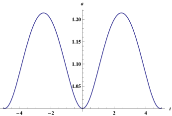
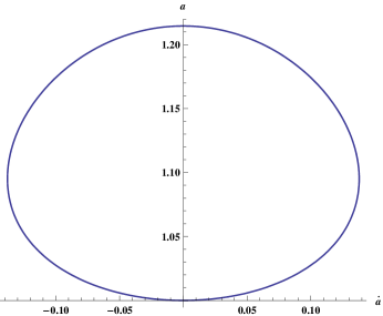
Figure 1: The evolutionary curve of the scale factor with time (left) and the phase diagram in space ($a$, $\dot{a}$) (right) for $\omega=1/3$.

To more study, we consider the effects of vacuum energy in the Rastall theory on the dynamics of the universe. As an example, we study the case where the energy content consists of vacuum energy, which we put $\omega_{\Lambda}=-1$ and $\rho_{\Lambda}=A/a^{4}$, in addition to a relativistic matter with an equation-of-state parameter $\omega=1/3$. Using these equation of state parameters in equation (VI) we obtain

$$3a^{3}\ddot{a}+3a^{2}\dot{a}^{2}+3a^{2}-\frac{2A}{(1-4\lambda)}=0$$ (44)

From the above equation the corresponding scale factor of Einstein static solution is given by $a_{Es}^{2}=2A/3(1-4\lambda)$. Obviously, phase space trajectories which is beginning precisely on the Einstein static fixed point remain there indeterminately. From another point of view, trajectories which are creating in the vicinity of this point would oscillate indefinitely near this solution. An example of such a universe trajectory using initial conditions given by $a(0)=1$ and $\dot{a}(0)=0$, with $A=1.1$ and $\lambda=0.1$ has been plotted in Fig. 1.

VII Conclusion

We have discussed the existence and stability of the Einstein static universe in the presence of perfect fluid with a vacuum energy corresponding to conformally-invariant fields through the Rastall theory of gravity. Using the fix point method, we have found that the scale factor of Einstein static universe for closed deformed isotropic and homogeneous FLRW universe depends on the coupling parameter $\lambda$ between the energy-momentum tensor and the gradient of Ricci scalar. Also, we have determined the allowed intervals for the equation of state parameters related to the vacuum energy such that the Einstein universe is stable, while it is dynamically belonging to a center equilibrium point. The motivation for study of such a solution is its essential role in the construction of non-singular emergent oscillatory model which is past eternal, and hence can resolve the singularity problem in the standard cosmological scenario.

References

- (1) P. Rastall, Phys. Rev. D 6 (1972) 3357.
- (2) P. Rastall, Can. J. Phys. 54 (1976) 66.
- (3) Vladimir Majernik and Lukas Richterek, arXiv:gr-qc/0610070.
- (4) N. D. Birrell and P. C. W. Davies, Quantum Fields in Curved Space, Cambridge University Press, Cambridge (1982).
- (5) T. Koivisto, Class. Quant. Grav. 23 (2006) 4289.
- (6) O. Minazzoli, Phys. Rev. D 88 (2013) 027506.
- (7) T. Harko, F. S. Lobo, S. Nojiri S, S. D. Odintsov, Phys. Rev. D 84 (2011) 024020.
- (8) T. Harko T, F.S. Lobo, Galaxies 2 (2014) 410.
- (9) G.W. Gibbons and S.W. Hawking, Phys. Rev. D 15 (1977) 2738.
-
(10)
L. Parker, Phys. Rev. D 3 (1971) 346;
L. Parker, Phys. Rev. D 3 (1971) 2546. - (11) L. H. Ford, Phys. Rev. D 35 (1987) 2955.
- (12) C. E. M. Batista, M. H. Daouda, J. C. Fabris, O. F. Piattella and D. C. Rodrigues, Phys. Rev. D 85 (2012) 084008.
- (13) S. H. Pereira, C. H. G. Bessa and J. A. S. Lima, Phys. Lett. B 690 (2010) 103.
- (14) S. Calogero, J. Cosm. Astrop. Phys 11 (2011) 016.
- (15) S. Calogero and H. Velten, J. Cosm. Astrop. Phys 11(2013) 025 .
- (16) H. Velten and S. Calogero, arXiv:1407.4306.
- (17) E. R. Bezerra de Mello, J. C. Fabris and B. Hartmann, Class. Quan. Grav. 32(2015) 085009.
- (18) A. M. Oliveira, H. E. S. Velten, J. C. Fabris and L. Casarini, Phys. Rev. D 92 (2015) 044020.
- (19) C. E. M. Batista, J. C. Fabris, O. F. Piattella and A. M. Velasquez-Toribio, Eur. Phys. J. C 73(2013) 2425.
- (20) J. C. Fabris, O. F. Piattella, D. C. Rodrigues and M. H. Daouda, AIP Conf. Proc. 1647 (2015) 50.
- (21) M. Capone, V. F. Cardone and M. L. Ruggiero, J. Phys. Conf. Ser. 222 (2010) 012012.
- (22) J. C. Fabris, O. F. Piattella, D. C. Rodrigues, C. E. M. Batista and M. H. Daouda, Int. J. Mod. Phys. Conf. Ser. 18(2012) 67.
- (23) J. P. Campos, J. C. Fabris, R. Perez, O. F. Piattella and H. Velten, Eur. Phys. J. C 73 (2013) 2357.
- (24) J. C. Fabris, M. H. Daouda and O. F. Piattella, Phys. Lett. B 711 (2012) 232.
- (25) J. C. Fabris, arXiv:1208.4649v1.
- (26) H. Moradpour, Phys. Lett. B 757 (2016) 187.
- (27) A. S .Al-Rawaf and M. O. Taha, Phys. Lett. B 366 (1996) 69.
- (28) A. S. Al-Rawaf and M. O. Taha, Gen. Rel. Grav. 28 (1996) 935.
- (29) G. F. R. Ellis and R. Maartens, Class. Quant. Grav. 21 (2004) 223.
- (30) G. F. R. Ellis, J. Murugan and C. G. Tsagas, Class. Quant. Grav. 21, 233 (2004).
-
(31)
S. Carneiro and R. Tavakol, Phys. Rev. D 80 (2009) 043528, arXiv: 0907.4795;
C. G. Boehmer, Class. Quant. Grav. 21 (2004) 1119. - (32) D. J. Mulryne, R. Tavakol, J. E. Lidsey and G. F. R. Ellis, Phys. Rev. D 71 (2005) 123512.
- (33) L. Parisi, M. Bruni, R. Maartens and K. Vandersloot, Class. Quant. Grav. 24 (2007) 6243.
- (34) P. Wu and H. Yu and J. Cosmol. Astro. Phys. 05 (2009) 007, arXiv:0905.3116.
- (35) J. E. Lidsey and D. J. Mulryne, Phys. Rev. D 73 (2006) 083508.
-
(36)
C. G. Boehmer, L. Hollenstein and F. S. N. Lobo, Phys. Rev. D 76 (2007) 084005;
N. Goheer, R. Goswami and P. K. S. Dunsby, Class. Quant. Grav. 26 (2009) 105003, arXiv: 0809.5247;
S. del Campo, R. Herrera and P. Labrana, JCAP 0711 (2007) 030;
R. Goswami, N. Goheer and P. K. S. Dunsby, Phys. Rev. D 78 (2008) 044011;
U. Debnath, Class. Quant. Grav. 25 (2008) 205019 ;
B. C. Paul and S. Ghose, arXiv: 0809.4131. - (37) S. S. Seahra and C. G. Bohmer, Phys. Rev. D 79 (2009) 064009.
- (38) C. G. Boehmer and F. S. N. Lobo, Phys. Rev. D 79 (2009) 067504, arXiv: 0902.2982
- (39) J. D. Barrow, G. Ellis, R. Maartens and C. Tsagas, Class. Quant. Grav. 20 (2003) L155 .
- (40) T. Clifton and J. D. Barrow, Phys. Rev. D 72, 123003 (2005).
- (41) J. D. Barrow and C. G. Tsagas, Class. Quant. Grav. 26 (2009) 195003, arXiv:0904.1340.
-
(42)
C. G. Boehmer, L. Hollenstein, F. S. N. Lobo and S. S. Seahra, arXiv:1001.1266;
C. G. Boehmer, F. S. N. Lobo and Nicola Tamanini, Phys. Rev. D 88 (2013) 104019. - (43) A. Odrzywolek, Phys. Rev. D 80 (2009) 103515 .
- (44) C. G. Boehmer and F. S. N. Lobo, Eur. Phys. J. C 70 (2010) 1111, arXiv:0909.3986.
- (45) P. Wu and H. Yu, Phys. Rev. D 81 (2010) 103522, arXiv: 0909.2821.
- (46) J. -T. Li, C. -C. Lee and C. -Q. Geng, Eur. Phys. J. C 73, 2315 (2013).
- (47) K. Atazadeh, Y. Heydarzade and F. Darabi, Phys. Lett. B 732 (2014) 223.
-
(48)
L. Parisi, N. Radicella and G. Vilasi, Phys. Rev. D 86 (2012) 024035;
M. Mousavi and F. Darabi, Nucl. Phys. B 919 (2017) 523, arXiv:1607.04377. - (49) F. F Yuan and P. Huang, Class. Quan. Grav. 34 (2017) 077001.
-
(50)
John. D. Barrow, G. F. R. Ellis, R. Maartens, C. G. Tsagas
Class. Quant. Grav. 20 (2003) 155 ;
P. K. S. Dunsby, B. A. Basset and G. F. R. Ellis, Class. Quan. Grav. 14 (1997) 1215;
A. D. Challinor, Class. Quant. Grav. 17 (2000) 871;
R. Maartens, C. G. Tsagas, and C. Ungarelli, Phys. Rev. D 63 (2001) 123507.