Generalized Phase Representation of
Integrate-and-Fire Models

Abstract

The quadratic integrate-and-fire (QIF) model captures the normal form bifurcation dynamics of Type-I neurons found in cortex. Remarkably, this model is known to have a dual equivalent representation in terms of phase, called the $\theta$-model, which has advantages for numerical simulations and analysis over the QIF model. Here, I investigate the nature of the dual representation and derive the general phase model expression for all integrate-and-fire models. Moreover, I show the condition for which the phase models exhibit discontinuous onset firing rate, the hallmark of Type-II spiking neurons.

1 Introduction

Integrate-and-fire models provide the simplest dynamic descriptions of biological neurons that produce brief pulse signals to communicate, called spikes. They abstract out the complex biological mechanism of spike generation with a simple threshold-reset process [1, 2], which allows efficient analysis and simulation of spiking neural network models.

Generally, an integrate-and-fire model is described by a continuous subthreshold dynamics and a discontinuous threshold-reset process:

$$\dot{x} =f(x)+I (\text{for }x<x_{+})$$ (1)

$$x \to x_{-} (\text{for }x=x_{+})$$

where $x$ represents the neuron’s internal state, $I(t)$ is the net-input (i.e. including rheobase) and $x_{+},~{}x_{-}$ are the threshold and the reset, respectively. For example, $f(x)=|x|$, $x_{+}=0$, $x_{-}=-1$ describes the leaky integrate-and-fire model [3].

An interesting example is the quadratic integrate-and-fire (QIF) model, defined by $f(x)=x^{2}$ and the threshold and reset at infinity: $x_{\pm}=\pm\infty$ [4]. Remarkably, this model is known to have a dual representation in terms of phase, called the $\theta$-model [5, 6]:

$$\dot{\theta} =(1-I)\sin(\theta)^{2}+I (\text{for }\theta<\pi/2)$$

$$\theta \to-\pi/2 (\text{for }\theta=\pi/2)$$

which transforms to QIF through the mapping $x=\tan(\theta)$. This phase representation maps the infinite real line to a unit circle $S^{1}$ through one-point compactification [7, 8] (see section 4.2), providing the canonical model for Type-I cortical neurons that exhibit SNIC bifurcations (saddle-node bifurcation on an invariant circle) [6]. Note that the phase representation removes the cumbersome infinities involved with the QIF model, as well as effectively removing the discontinuous threshold-reset process, due to the the periodicity of the model: $\sin(\theta)^{2}=\sin(\theta+\pi)^{2}$. Thus, the resulting phase dynamics is smooth and bounded, which is advantageous for numerical simulations and analysis of spiking neural network dynamics [9, 10, 11, 12], as well as optimization [13, 14].

However, the mathematical implications and the generalized form of the dual representation has not been investigated for general integrate-and-fire models. In this manuscript, I investigate the nature of the dual representation and derive the following generalized phase dynamics for all integrate-and-fire models:

$$\dot{y} =(1-I)\,g(y)+I (\text{for }y<y_{+})$$ (2)

$$y \to y_{-} (\text{for }y=y_{+})$$

which transforms to eq (1) through a corresponding mapping function:

$$x=h(y).$$

2 Derivation

Here, I introduce the idea of representative phase and dual ODEs to derive the dual form eq (2) of the integrate-and-fire dynamics.

2.1 Representative phase

The nonlinear function $f(x)$ of the integrate-and-fire models eq (1) is assumed to have a well-defined minimum value. Without loss of generality, a normalized form can be imposed to set the minimum of $f(x)$ at the origin, such that $\min f(x)=f(0)=0$, with the threshold $x_{+}\geq 0$, and the reset $x_{-}<0$. Also, $f(x)$ is assumed to diverge to infinity in the limit $x\to\pm\infty$, but not for finite $x$: $f(x)<\infty,~{}\forall|x|<\infty$. Note that a positive input $I>0$ drives the dynamics to fire spikes repeatedly (oscillatory regime), whereas a negative input $I<0$ ceases such on-going activities (excitable regime).

Now, consider the integrate-and-fire dynamics eq (1) under a constant unit input $I=1$ as a representative case, and define $y$ as the phase of this representative dynamics: i.e.

$$\frac{dx}{dy} =\tilde{f}(x),$$ (3)

$$\text{where}~{}~{}~{}~{}~{}~{}~{}~{}~{}\tilde{f}(x) \equiv f(x)+1.~{}~{}~{}~{}~{}~{}~{}~{}~{}~{}~{}~{}~{}~{}$$

Note that $y$ is defined as a time-like variable, and $\tilde{f}(x)\geq 1$ for $\forall x$.

By definition, the phase dynamics under is $\dot{y}=1$ for the constant unit input $I=1$. Generalizing the phase dynamics to arbitrary time-varying input $I(t)$ requires finding the dual ODE of eq (3).

2.2 Dual ODEs

Dual ODEs are defined here as a pair of ordinary differential equations (ODEs)

$$\frac{dx}{dy} =\tilde{f}(x)$$

$$\frac{dy}{dx} =\tilde{g}(y)$$

that describe an identical relationship between $x$ and $y$. Such pairs can always be found for monotonic relationships: i.e. $\tilde{f}(x),\tilde{g}(y)>0$. In integral forms, the relationship is expressed as

$$x =\int_{0}^{y}\frac{du}{\tilde{g}(u)}\equiv h(y)$$ (4)

$$y =\int_{0}^{x}\frac{du}{\tilde{f}(u)}\equiv h^{-1}(x).$$ (5)

That is, the integral of $1/\tilde{g}$ is the inverse function of the integral of $1/\tilde{f}$. Note that the condition $h(0)=0$ is imposed at the origin without loss of generality.

2.3 Legendre transform

The problem of finding the dual of an ODE is closely related to Legendre transform. Legendre transform of a convex function $H(x)$ is [15]

$$H^{*}(y)=\min_{x}\,yx-H(x),$$ (6)

where $y$ is the dual variable of $x$. The mapping between $x$ and $y$ is described by the first order derivatives

$$y =H^{\prime}(x)~{}\equiv h^{-1}(x)$$

$$x ={H^{*}}^{\prime}(y)\equiv h(y),$$

which can be identified with eq (4,5) to yield

$$H^{\prime\prime}(x) ={1}/{\tilde{f}(x)}$$

$${H^{*}}^{\prime\prime}(y) ={1}/{\tilde{g}(y)}.$$

This result links Legendre transform to the dual ODE problem. Moreover, these second order derivatives are well known to be reciprocal to each other:

$$H^{\prime\prime}(x){H^{*}}^{\prime\prime}(y)=\frac{1}{\tilde{f}(x)\,\tilde{g}(y)}=1.$$ (7)

2.4 Generalized phase dynamics

For arbitrary time-varying input $I(t)$, the phase dynamics generalizes to the following form

$$\dot{y}=\frac{dx}{dt}\frac{dy}{dx} =(f(x)+I)\tilde{g}(y),~{}~{}~{}$$ (8)

where $$\frac{dy}{dx} =\tilde{g}(y)$$

is the dual ODE of eq (3), as determined by Legendre transform.

According to the reciprocity condition eq (7) and $f(x)=\tilde{f}(x)-1$, equation (8) simplifies to

$$\dot{y} =1+(I-1)\,\tilde{g}(y)$$

$$=(1-I)\,g(y)+I,$$

which derives the generalized phase dynamics eq (2). Here, $g(y)\equiv 1-\tilde{g}(y)$ is defined to describe the intrinsic phase dynamics under the null input, $I=0$.

3 Examples

The above result generalizes the dual relationship between the QIF model and the $\theta$-model to all integrate-and-fire models of the form eq (1). Some examples are shown here. See Figure 1 and Table 1.

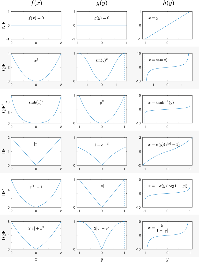
Figure 1: Dynamic functions $f(x)$ of various integrate-and-fire models, the corresponding dual functions $g(y)$ of the phase dynamics, and the mapping functions $x=h(y)$ are shown. Dashed lines indicate where $h(y)$ diverge: $\lim_{x\to\pm\infty}h^{-1}(x)$. $\sigma(\cdot)$ is the sign function.

• NIF Non-leaky integrate-and-fire model: Self-dual.

  $$~{}\dot{x} =I,~{}~{}~{}~{} \dot{y} =I~{}~{}~{}~{}~{}~{}~{}~{}~{}~{}~{}~{}~{}~{}~{}~{}~{}~{}~{}~{}~{}~{}~{}~{}~{}~{}~{}~{}$$

• QIF Quadratic integrate-and-fire model.

  $$~{}~{}~{}~{}~{}\dot{x} =x^{2}+I, \dot{y} =(1-I)\sin(y)^{2}+I~{}~{}$$

• QIF^∗ Quadratic phase dynamics model.

  $$~{}~{}~{}~{}~{}~{}~{}~{}~{}~{}~{}~{}~{}~{}\dot{x} =\sinh(x)^{2}+I, \dot{y} =(1-I)y^{2}+I~{}~{}~{}~{}~{}~{}~{}~{}~{}~{}~{}~{}~{}~{}~{}~{}~{}~{}~{}~{}$$

• LIF Linear (or Leaky) integrate-and-fire model (symmetrized).

  $$~{}~{}~{}~{}~{}~{}~{}~{}~{}\dot{x} =|x|+I,~{}~{}~{}~{} \dot{y} =(1-I)(1-e^{-|y|})+I$$

• LIF^∗ Linear phase dynamics model (symmetrized).

  $$~{}~{}~{}~{}~{}~{}~{}~{}~{}~{}\dot{x} =e^{|x|}-1+I, \dot{y} =(1-I)|y|+I~{}~{}~{}~{}~{}~{}~{}~{}~{}~{}~{}~{}~{}~{}~{}$$

• LQIF Linear-Quadratic integrate-and-fire model (symmetrized).

  $$~{}~{}~{}~{}~{}~{}~{}~{}~{}~{}~{}~{}\dot{x} =2|x|+x^{2}+I, \dot{y} =(1-I)(2|y|-y^{2})+I~{}~{}~{}~{}$$

	NIF	QIF	QIF∗	LIF	LIF∗	LQIF
$\tilde{f}(x)$	$1$	$1+x^{2}$	$\cosh(x)^{2}$	$1+|x|$	$e^{|x|}$	$(1+|x|)^{2}$
$\tilde{g}(y)$	$1$	$\cos(y)^{2}$	$1-y^{2}$	$\displaystyle e^{-|y|}$	$1-|y|$	$(1-|y|)^{2}$
$h(y)$	$y$	$\tan(y)$	$\tanh^{-1}(y)$	$\sigma(y)(e^{|y|}-1)$	$-\sigma(y)\log(1-|y|)$	$\displaystyle\frac{y}{1-|y|}$

Table 1: Representative dynamic functions $\tilde{f}(x)$ of various integrate-and-fire models under unit input $I=0$, the corresponding dual functions $\tilde{g}(y)$ of the phase dynamics, and the mapping functions $x=h(y)$ are shown. $\sigma(\cdot)$ is the sign function.

4 Properties of the phase model

4.1 Phase dynamics function $g(y)$

The reciprocity condition eq (7) yields the following relationships between the dynamics functions of the dual representations

$$g(y)=\frac{f(x)}{1+f(x)}$$ (9)

and between their derivatives

$$\frac{dg}{dy}=\frac{df/dx}{1+f}=\frac{d}{dx}\log(1+f),$$ (10)

where $x=h(y)$ is implied.

Since ${f}(x)\geq 0$, $g(y)$ is bounded by $0\leq{g}(y)\leq 1$, with the minimum at the origin, $f(0)=g(0)=0$. In the limit $x\to\pm\infty$, $g(y)$ approaches 1 as $f(x)$ diverges to infinity.

The derivatives ${dg}/{dy}\approx{df}/{dx}$ are similar near the origin, since $\log(1+f(x))\approx f(x)$ for $|x|\ll 1$. In the limit $x\to\pm\infty$, $dg/dy$ remains finite only if $f(x)$ is an exponentially growing function (e.g. QIF^∗ and LIF^∗). Otherwise, the derivative of $\log(1+f(x))$ approaches zero in the limit (e.g. polynomial $f(x)$: QIF, LIF, and LQIF).

4.2 Compatification

The phase $y=h^{-1}(x)$ describes the time it takes for the representative dynamics $\dot{x}=\tilde{f}(x)$ to reach $x$ from the origin. Therefore, for model dynamics that diverges to infinity within finite time, the phase $y_{\pm}$ that corresponds to the threshold/reset $x_{\pm}$ at infinity is finite (e.g. QIF, QIF^∗, LIF^∗, LQIF). Thus, for these fast diverging models, the phase representation shrinks the infinite real line to an open interval $(y_{-},y_{+})$. The open interval can then be topologically morphed into a circle $S^{1}$ by bringing the ends of the interval together and adding a single "point at infinity", a process called one-point compactification [7, 8].

The compactification of phase representations resolves the inconvenience of simulating diverging dynamics over the infinite domain. Moreover, it removes the discontinuity of the threshold-reset process by equating the threshold phase with the reset phase, at which the dynamics is identical: $g(y_{-})=g(y_{+})=1$.

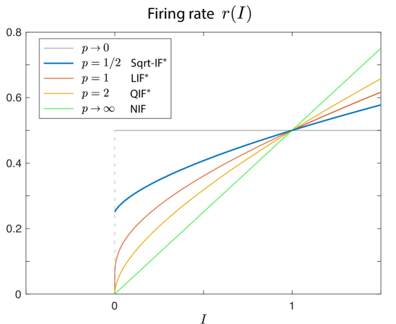
Figure 2: Firing rate of various phase dynamics models of the form $g(y)=|y|^{p}$. The limit $p\to\infty$ corresponds to the NIF model. For $p\geq 1$, the onset firing rate is $r(0)=0$. For $p<1$, the models exhibit non-zero onset firing rate, with discontiuous F-I cuves at $I=0$.

	NIF	QIF∗	LIF∗	Sqrt-IF∗	LQIF
${g}(y)$	$0$	$y^{2}$	$|y|$	$\sqrt{|y|}$	$2|y|-y^{2}$
$r(I)$	$\displaystyle\frac{I}{2}$	$\displaystyle\frac{1}{2}\frac{\sqrt{(I-1)I}}{\tanh^{-1}(\sqrt{(I-1)/I})}$	$\displaystyle\frac{1}{2}\frac{I-1}{\log I}$	$\displaystyle\frac{1}{4}\frac{(I-1)^{2}}{1+I(\log I-1)}$	$\displaystyle\frac{1}{2}\frac{\sqrt{I-1}}{\tan^{-1}(\sqrt{I-1})}$

Table 2: The firing rate $r(I)$ of various phase dynamics models. $I\geq 0$. $y_{\pm}=\pm 1$.

4.3 Firing rate

For positive constant input $I>0$, integrate-and-fire models exhibit periodic spiking activities. The spiking period can be calculated as

$$T(I)=\int_{x_{-}}^{x_{+}}\frac{dx}{f(x)+I}=\int_{y_{-}}^{y_{+}}\frac{dy}{(1-I)g(y)+I}.$$

Note that the spiking period for unit input is always $T(1)=y_{+}-y_{-}$ for all models.

The inverse of period is called the firing rate: $r(I)\equiv 1/T(I)$. For negative constant input $I<0$, the firing rate is $r(I)=0$. The firing rate functions are shown in Table 2 for various integrate-and-fire models.

Figure 2 shows the firing rate plotted against the input, called the F-I curves. In many models, the firing rate continuously decreases to zero with the input, the defining characteristics of Type-I cortical neurons. Remarkably, however, the square-root phase dynamics model (Sqrt-IF^∗), defined by $g(y)=\sqrt{|y|}$, exhibits non-zero firing rate at onset $I=0$, the hallmark of Type-II neurons [16].

More generally, the onset firing rate of monomial phase dynamics models $g(y)=|y|^{p}$ is

$$\lim_{I\to 0^{+}}r(I) =\frac{1-p}{2} (\text{for }p<1)$$

$$=0 (\text{for }p\geq 1)$$

(with $y_{\pm}=\pm 1$), where the limit is taken from the positive side. Thus, the F-I curves of monomial phase models of $p<1$ exhibit Type-II-like discontinuities at onset $I=0$.

The onset characteristics generalizes to other models whose phase dynamics function approximates $g(y)\approx|y|^{p}$ near the origin. For example, the integrate-and-fire model with $f(x)=e^{\sqrt{2|x|}}-1$ exhibits non-zero onset firing rate, since its phase dynamics is $g(y)\approx\sqrt{2|y|}$ for small $|y|\ll 1$. Also, QIF^∗’s firing rate is approximated by QIF’s rate $r(I)=\sqrt{I}/\pi$ near the onset, and LIF^∗’s firing rate is approximated by LIF’s rate $r(I)=[2\log(1+1/I)]^{-1}$ near the onset ($x_{\pm}=\pm 1$).

5 Summary

I introduced the formal definition for the phase representation of integrate-and-fire models and derived the generalized expression for the phase dynamics models. The compactified phase representation for integrate-and-fire models would facilitate efficient simulations and analysis of large scale spiking neural network dynamics.

Analysis of the phase representation revealed a new class of integrate-and-fire models that blur the distinction between Type-I and Type-II neurons [16]. Despite the discontinuous onset of F-I curves, however, these models do not truly qualify as Type-II, since their phase response curves are strictly positive (not shown here), and they exhibit SNIC bifurcations rather than Hopf or saddle-node-off-limit-cycle bifurcations. Remarkably, however, these models can also exhibit supercritical Hopf bifurcation with sustained subthreshold oscillations when paired with an adaptation process (not shown here), which require further investigation.

Acknowledgments

The author would like to thank Bard Ermentrout for insightful discussion.

References

- [1] Louis Lapicque. Recherches quantitatives sur l’excitation électrique des nerfs traitée comme une polarisation. J. Physiol. Pathol. Gen., 9:620–635, 1907.
- [2] Eugene M Izhikevich. Dynamical systems in neuroscience. MIT press, 2007.
- [3] Richard B Stein. A theoretical analysis of neuronal variability. Biophysical Journal, 5(2):173–194, 1965.
- [4] Peter E Latham, BJ Richmond, PG Nelson, and S Nirenberg. Intrinsic dynamics in neuronal networks. i. theory. Journal of neurophysiology, 83(2):808–827, 2000.
- [5] Bard Ermentrout. Type i membranes, phase resetting curves, and synchrony. Neural computation, 8(5):979–1001, 1996.
- [6] Bard Ermentrout. Ermentrout-kopell canonical model. Scholarpedia, 3(3):1398, 2008.
- [7] Paul Alexandroff. Über die metrisation der im kleinen kompakten topologischen räume. Mathematische Annalen, 92(3):294–301, 1924.
- [8] Wikipedia. Compactification (mathematics) — wikipedia, the free encyclopedia, 2017. [Online; accessed 10-November-2017].
- [9] Michael Monteforte and Fred Wolf. Dynamical entropy production in spiking neuron networks in the balanced state. Physical review letters, 105(26):268104, 2010.
- [10] Guillaume Lajoie, Kevin K Lin, and Eric Shea-Brown. Chaos and reliability in balanced spiking networks with temporal drive. Physical Review E, 87(5):052901, 2013.
- [11] Guillaume Lajoie, Jean-Philippe Thivierge, and Eric Shea-Brown. Structured chaos shapes spike-response noise entropy in balanced neural networks. Frontiers in computational neuroscience, 8, 2014.
- [12] Nikita Novikov and Boris Gutkin. Robustness of persistent spiking to partial synchronization in a minimal model of synaptically driven self-sustained activity. Physical Review E, 94(5):052313, 2016.
- [13] Dongsung Huh and Terrence J Sejnowski. Gradient descent for spiking neural networks. arXiv preprint arXiv:1706.04698, 2017.
- [14] Sam McKennoch, Thomas Voegtlin, and Linda Bushnell. Spike-timing error backpropagation in theta neuron networks. Neural computation, 21(1):9–45, 2009.
- [15] Royce KP Zia, Edward F Redish, and Susan R McKay. Making sense of the legendre transform. American Journal of Physics, 77(7):614–622, 2009.
- [16] Frances K Skinner. Moving beyond type i and type ii neuron types. F1000Research, 2, 2013.