A Study Of Optimal False Information Injection Attack On Dynamic State Estimation in Multi-Sensor Systems

Jingyang Lu and Ruixin Niu
Abstract

In this paper, the impact of false information injection is investigated for linear dynamic systems with multiple sensors. It is assumed that the system is unsuspecting the existence of false information and the adversary is trying to maximize the negative effect of the false information on Kalman filter’s estimation performance. The false information attack under different conditions is mathematically characterized. For the adversary, many closed-form results for the optimal attack strategies that maximize Kalman filter’s estimation error are theoretically derived. It is shown that by choosing the optimal correlation coefficients among the bias noises and allocating power optimally among sensors, the adversary could significantly increase Kalman filter’s estimation errors. To be concrete, a target tracking system is used as an example in the paper. From the adversary’s point of view, the best attack strategies are obtained under different scenarios, including a single-sensor system with both position and velocity measurements, and a multi-sensor system with position and velocity measurements. Under a constraint on the total power of the injected bias noises, the optimal solutions are solved from two perspectives: trace and determinant. Numerical results are also provided in order to illustrate the effectiveness of the proposed attack strategies.

I Introduction

System state estimation in the presence of an adversary that injects false information into sensor readings has attracted much attention in wide application areas, such as target tracking with compromised sensors, secure monitoring of dynamic electric power systems and radar tracking and detection in the presence of jammers [1]. This topic has been studied in [2, 3, 4, 5, 6, 7, 8, 9]. In [2], the problem of taking advantage of the power system configuration to introduce arbitrary bias to the system without being detected was investigated and inspired many researchers further study false information injection along this direction. [3] shows the impact of malicious attacks on real-time electricity market concerning the locational marginal price and how the attackers can make profit by manipulating certain values of the measurements. Some certain strategies are also provied to find the optimal single attack vector. The relationship between the attackers and the control center was discussed in [4], where both the adversary’s attacking strategies and the control center’s detection algorithms have been proposed. Refer to [5] and [6] for more about false information attacks on the electricity market. Inspired by [2], the data frame attack in which deleting the comprised sensors the defender system detects will make the system unobservable was formulated as a quadratically constrained quadratic program (QCQP) in [7]. In [8, 9], the relation between a target and a MIMO radar was characterized as a two-person zero-sum game. However, in the aforementioned publications, only the problem of static system state estimation has been considered.

In this paper, for a linear dynamic system, we analyze the impact of the injected false information on Kalman filter’s state estimation performance over time, which has not got much attention in the literature. Some related publications exist on sensor management [10, 11, 12], where the problem of arranging the sensors to minimize the covariance of the state estimation error so that a more accurate state estimate can be obtained is investigated. This problem is clearly opposite to the problem we study in the paper, where the goal for the adversary is to maximize the mean square state estimation error matrix, and to confuse Kalman filter. In [13], the problem of sensor bias estimation and compensation for target tracking has been addressed. Interested readers are referred to [13] and the references therein for details.

In [14], we have studied the impact of the injected biases on a Kalman filter’s estimation performance, showing that if the false information is injected at a single time, its impact converges to zero as time goes on; if the false information is injected into the system continuously, the estimation error tends to reach a steady state. In [15], we have found the best strategies for the adversary to attack Kalman filter system from the perspective of the trace of the mean squared error (MSE) matrix, and obtained some close-form results. Also in [16], based on the previous work, the problem is further refined regarding the determinant of MSE matrix, which the correlation among the elements is taken into consideration. In [17, 18], the Kalman filter system has been investigated regarding the system robustness in the case where sensor reading is continuously jammed by the false information using Greedy search and dynamic programming. However, the it is of great challenge to find the closed form solution in term of determinant of the MSE matrix and optimal solution to the case in which the Kalman filter system is compromised by the false information continuously. Considering the problems mentioned above, in this paper, our goal is to find the closed form optimal attack strategy for the adversary, which maximizes the impact of the false information injection on Kalman filter’s state estimation from the determinant perspective. By adopting the objective function as the determinant of the MSE matrix, we change the problem significantly. As shown later in the paper, the optimal attack strategy that maximizes the determinant of the MSE matrix is a function of Kalman filter’s state estimation covariance and hence ”adaptive” to Kalman filter; whereas that maximizing the trace of the MSE matrix is not a function of Kalman filter’s state estimation covariance. Previous works concentrated more on the situation where the adversary attacks the system by a single shot. In this paper, the problem of continuous attack is also investigated.

The rest of paper is organized as follows. Section II generally describes the discrete-time linear dynamic system. Section III mathematically characterizes the impact of determined or random false information on Kalman filter’s system. Section IV and V analyze how to get the best strategy to attack Kalman filter’s system from trace and determinant cases standing from the perspective of the adversary. Under the constraint on the adversary’s total sensor bias noise power, different strategies are proposed to maximize Kalman filter’s mean squared state estimation error for different scenarios. Section VI provides the simulation results and Section VII concludes the paper.

II Kalman filter System

III System Model

The discrete-time linear dynamic system can be described as below,

𝐱k+1=𝐅k𝐱k+𝐆k𝐮k+𝐯ksubscript𝐱𝑘1subscript𝐅𝑘subscript𝐱𝑘subscript𝐆𝑘subscript𝐮𝑘subscript𝐯𝑘\mathbf{x}_{k+1}=\mathbf{F}_{k}\mathbf{x}_{k}+\mathbf{G}_{k}\mathbf{u}_{k}+\mathbf{v}_{k} (1)

where 𝐅ksubscript𝐅𝑘{\bf F}_{k} is the system state transition matrix, 𝐱ksubscript𝐱𝑘\mathbf{x}_{k} is the system state vector at time k𝑘k, 𝐮ksubscript𝐮𝑘\mathbf{u}_{k} is a known input vector, 𝐆ksubscript𝐆𝑘\mathbf{G}_{k} is the input gain matrix, and 𝐯ksubscript𝐯𝑘\mathbf{v}_{k} is a zero-mean white Gaussian process noise with covariance matrix E[𝐯k𝐯kT]=𝐐k𝐸delimited-[]subscript𝐯𝑘superscriptsubscript𝐯𝑘𝑇subscript𝐐𝑘E[\mathbf{v}_{k}\mathbf{v}_{k}^{T}]=\mathbf{Q}_{k}. Let us assume that M𝑀M sensors are used by the linear system. The measurement at time k𝑘k collected by sensor i𝑖i is

𝐳k,i=𝐇k,i𝐱k,i+𝐰k,isubscript𝐳𝑘𝑖subscript𝐇𝑘𝑖subscript𝐱𝑘𝑖subscript𝐰𝑘𝑖\mathbf{z}_{k,i}=\mathbf{H}_{k,i}\mathbf{x}_{k,i}+\mathbf{w}_{k,i} (2)

with 𝐇k,isubscript𝐇𝑘𝑖\mathbf{H}_{k,i} being the measurement matrix, and 𝐰k,isubscript𝐰𝑘𝑖\mathbf{w}_{k,i} a zero-mean white Gaussian measurement noise with covariance matrix E[𝐰k,i𝐰k,iT]=𝐑k,i𝐸delimited-[]subscript𝐰𝑘𝑖superscriptsubscript𝐰𝑘𝑖𝑇subscript𝐑𝑘𝑖E[\mathbf{w}_{k,i}\mathbf{w}_{k,i}^{T}]=\mathbf{R}_{k,i}, for i=1,,M𝑖1𝑀i=1,\cdots,M. We further assume that the measurement noises are independent across sensors. The matrices 𝐅ksubscript𝐅𝑘\mathbf{F}_{k}, 𝐆ksubscript𝐆𝑘\mathbf{G}_{k}, 𝐇k,isubscript𝐇𝑘𝑖\mathbf{H}_{k,i}, 𝐐ksubscript𝐐𝑘\mathbf{Q}_{k}, and 𝐑k,isubscript𝐑𝑘𝑖\mathbf{R}_{k,i} are assumed to be known with proper dimensions. In this paper, we assume that a bias 𝐛k,isubscript𝐛𝑘𝑖\mathbf{b}_{k,i} is injected by the adversary into the measurement of the i𝑖ith sensor at time k𝑘k intentionally. Therefore, the measurement equation (2) becomes

𝐳k,i=𝐇k,i𝐱k+𝐰k,i+𝐛k,i=𝐳k,i+𝐛k,isubscriptsuperscript𝐳𝑘𝑖subscript𝐇𝑘𝑖subscript𝐱𝑘subscript𝐰𝑘𝑖subscript𝐛𝑘𝑖subscript𝐳𝑘𝑖subscript𝐛𝑘𝑖\displaystyle\mathbf{z}^{\prime}_{k,i}=\mathbf{H}_{k,i}\mathbf{x}_{k}+\mathbf{w}_{k,i}+\mathbf{b}_{k,i}=\mathbf{z}_{k,i}+\mathbf{b}_{k,i} (3)

where 𝐳k,isubscriptsuperscript𝐳𝑘𝑖\mathbf{z}^{\prime}_{k,i} is the corrupted measurement, 𝐛k,isubscript𝐛𝑘𝑖\mathbf{b}_{k,i} is either an unknown constant or a random variable independent of {𝐯k,i}subscript𝐯𝑘𝑖\{\mathbf{v}_{k,i}\} and {𝐰k,i}subscript𝐰𝑘𝑖\{\mathbf{w}_{k,i}\}.

For compactness, let us denote the system sensor observation as 𝐳k=[𝐳k1T,,𝐳kMT]Tsubscript𝐳𝑘superscriptsuperscriptsubscript𝐳𝑘1𝑇superscriptsubscript𝐳𝑘𝑀𝑇𝑇{\bf z}_{k}=[{\bf z}_{k1}^{T},\cdots,{\bf z}_{kM}^{T}]^{T}, which contains the observations from all the M𝑀M sensors. Similarly, let us denote the system bias vector as 𝐛k=[𝐛k1T,,𝐛kMT]Tsubscript𝐛𝑘superscriptsuperscriptsubscript𝐛𝑘1𝑇superscriptsubscript𝐛𝑘𝑀𝑇𝑇{\bf b}_{k}=[{\bf b}_{k1}^{T},\cdots,{\bf b}_{kM}^{T}]^{T} which includes the biases at all the M𝑀M sensors. Correspondingly, the measurement matrix becomes

𝐇k=[𝐇k1T,,𝐇kMT]Tsubscript𝐇𝑘superscriptsuperscriptsubscript𝐇𝑘1𝑇superscriptsubscript𝐇𝑘𝑀𝑇𝑇{\bf H}_{k}=[{\bf H}_{k1}^{T},\cdots,{\bf H}_{kM}^{T}]^{T} (4)

With these notations, it is easy to convert (2) and (3) into the following equations respectively.

𝐳k=𝐇k𝐱k+𝐰ksubscript𝐳𝑘subscript𝐇𝑘subscript𝐱𝑘subscript𝐰𝑘\mathbf{z}_{k}=\mathbf{H}_{k}\mathbf{x}_{k}+\mathbf{w}_{k} (5)

and

𝐳k=𝐳k+𝐛ksubscriptsuperscript𝐳𝑘subscript𝐳𝑘subscript𝐛𝑘\mathbf{z}^{\prime}_{k}=\mathbf{z}_{k}+\mathbf{b}_{k} (6)

Further, we have the measurement error covariance matrix corresponding to 𝐰ksubscript𝐰𝑘{\bf w}_{k} is

𝐑k=[𝐑k,1𝟎𝟎𝐑k,M]subscript𝐑𝑘delimited-[]subscript𝐑𝑘100subscript𝐑𝑘𝑀{\bf R}_{k}=\left[\begin{array}[]{lcr}{\bf R}_{k,1}&\cdots&{\bf 0}\\ \vdots&\ddots&\vdots\\ {\bf 0}&\cdots&{\bf R}_{k,M}\\ \end{array}\right] (7)

which is obtained by using the assumption that measurement noises are independent across sensors.

IV Impact of False Information Injection

In this paper, let us assume that the adversary attacks the system by injecting false information into the sensors while unaware of such attacks. We start with the case where biases (𝐛ksubscript𝐛𝑘{\bf b}_{k}) are continuously injected into the system starting from a certain time K𝐾K. Note that single injection is just a special case of continuous injection when 𝐛ksubscript𝐛𝑘{\bf b}_{k} are set to be nonzero at time K𝐾K and zero otherwise.

In the continuous injection case, Kalman filter’ extra state estimation error, which is caused by the continuous bias injection alone, is derived in [19] and provided as follows.

Proposition 1.

Kalman filter’s state estimation error at time K+N𝐾𝑁K+N is

𝐱^K+N|K+N𝐱K+N=𝐱^K+N|K+N𝐱K+N+m=0N(i=0m1𝐁K+Ni)𝐖K+Nm𝐛K+Nmsubscriptsuperscript^𝐱𝐾conditional𝑁𝐾𝑁subscript𝐱𝐾𝑁subscript^𝐱𝐾conditional𝑁𝐾𝑁subscript𝐱𝐾𝑁superscriptsubscript𝑚0𝑁superscriptsubscriptproduct𝑖0𝑚1subscript𝐁𝐾𝑁𝑖subscript𝐖𝐾𝑁𝑚subscript𝐛𝐾𝑁𝑚\displaystyle\begin{split}&{\hat{\mathbf{x}}^{\prime}_{K+N|K+N}}-\mathbf{x}_{K+N}={\hat{\mathbf{x}}_{K+N|K+N}}-\mathbf{x}_{K+N}\\ &+\sum_{m=0}^{N}\left(\prod_{i=0}^{m-1}\mathbf{B}_{K+N-i}\right)\mathbf{W}_{K+N-m}\mathbf{b}_{K+N-m}\\ \end{split} (8)

where 𝐱^K+N|K+Nsubscriptsuperscript^𝐱𝐾conditional𝑁𝐾𝑁\hat{\mathbf{x}}^{\prime}_{K+N|K+N} is Kalman filter’s state estimate in the presence of the bias sequence {𝐛k}subscript𝐛𝑘\{{\bf b}_{k}\}, 𝐱^K+N|K+Nsubscript^𝐱𝐾conditional𝑁𝐾𝑁\hat{\mathbf{x}}_{K+N|K+N} is Kalman filter’s state estimate in the absence of the bias,

𝐁K(𝐈𝐖K𝐇K)𝐅K1,subscript𝐁𝐾𝐈subscript𝐖𝐾subscript𝐇𝐾subscript𝐅𝐾1\mathbf{B}_{K}\triangleq\left(\mathbf{I}-\mathbf{W}_{K}\mathbf{H}_{K}\right)\mathbf{F}_{K-1}, (9)

𝐈𝐈{\bf I} is the identity matrix, and 𝐖Ksubscript𝐖𝐾\mathbf{W}_{K} is Kalman filter gain [20] at time K𝐾K. As a result, the extra state estimation error at time K+N𝐾𝑁K+N due to the continuous bias 𝐛ksubscript𝐛𝑘{\bf b}_{k} injected at and after time K𝐾K is

m=0N(i=0m1𝐁K+Ni)𝐖K+Nm𝐛K+Nm,superscriptsubscript𝑚0𝑁superscriptsubscriptproduct𝑖0𝑚1subscript𝐁𝐾𝑁𝑖subscript𝐖𝐾𝑁𝑚subscript𝐛𝐾𝑁𝑚\sum_{m=0}^{N}\left(\prod_{i=0}^{m-1}\mathbf{B}_{K+N-i}\right)\mathbf{W}_{K+N-m}\mathbf{b}_{K+N-m}, (10)

If {𝐛ksubscript𝐛𝑘{\bf b}_{k}} is a zero-mean, random, and independent sequence, the extra mean squared error (EMSE) at a particular time instant K+N𝐾𝑁K+N due to the bias alone is provided in the following proposition. Using the results from Proposition 1, the proof of Proposition 2 is provided as well.

Proposition 2.

When the bias sequence {𝐛k}subscript𝐛𝑘\{{\bf b}_{k}\} is zero mean, random, and independent over time, the EMSE𝐸𝑀𝑆𝐸EMSE at time K+N𝐾𝑁K+N due to the biases injected at and after time K𝐾K, denoted as 𝐀K+Nsubscript𝐀𝐾𝑁{\bf A}_{K+N}, is

𝐀K+N=m=0N𝐃m𝚺K+Nm𝐃mTsubscript𝐀𝐾𝑁superscriptsubscript𝑚0𝑁subscript𝐃𝑚subscript𝚺𝐾𝑁𝑚subscriptsuperscript𝐃𝑇𝑚\displaystyle\mathbf{A}_{K+N}=\sum_{m=0}^{N}\mathbf{D}_{m}{\bf\Sigma}_{K+N-m}\mathbf{D}^{T}_{m} (11)

where

𝐃m=(i=0m1𝐁K+Ni)𝐖K+Nmsubscript𝐃𝑚superscriptsubscriptproduct𝑖0𝑚1subscript𝐁𝐾𝑁𝑖subscript𝐖𝐾𝑁𝑚\displaystyle\mathbf{D}_{m}=\left(\prod_{i=0}^{m-1}\mathbf{B}_{K+N-i}\right)\mathbf{W}_{K+N-m} (12)

i=01𝐁K+Ni=𝐈superscriptsubscriptproduct𝑖01subscript𝐁𝐾𝑁𝑖𝐈\prod_{i=0}^{-1}\mathbf{B}_{K+N-i}={\bf I} is an identity matrix, and 𝚺K+Nmsubscript𝚺𝐾𝑁𝑚{\bf\Sigma}_{K+N-m} is the covariance matrix of 𝐛K+Nmsubscript𝐛𝐾𝑁𝑚\mathbf{b}_{K+N-m}.

Proof Sketches: Let us denote 𝐱~K+N|K+N=𝐱^K+N|K+N𝐱K+Nsubscript~𝐱𝐾conditional𝑁𝐾𝑁subscript^𝐱𝐾conditional𝑁𝐾𝑁subscript𝐱𝐾𝑁\tilde{\mathbf{x}}_{K+N|K+N}={\hat{\mathbf{x}}_{K+N|K+N}}-\mathbf{x}_{K+N} as Kalman filter’s state estimation error in the absence of any false information, and

𝐚m=(i=0m1𝐁K+Ni)𝐖K+Nm𝐛k+Nmsubscript𝐚𝑚superscriptsubscriptproduct𝑖0𝑚1subscript𝐁𝐾𝑁𝑖subscript𝐖𝐾𝑁𝑚subscript𝐛𝑘𝑁𝑚\mathbf{a}_{m}=\left(\prod_{i=0}^{m-1}\mathbf{B}_{K+N-i}\right)\mathbf{W}_{K+N-m}\mathbf{b}_{k+N-m} (13)

From (LABEL:eq:err), we can get

𝐀K+N=E[(𝐱~K+N|K+N+m=0N𝐚m)(𝐱~K+N|K+N+n=0N𝐚n)T]E(𝐱~K+N|K+N𝐱~K+N|K+NT)=E(𝐱~K+N|K+Nn=0N𝐚nT)+E(m=0N𝐚m𝐱~K+N|K+NT)+E(m=0Nn=0N𝐚m𝐚nT)=E(m=0Nn=0N𝐚m𝐚nT)subscript𝐀𝐾𝑁𝐸delimited-[]subscript~𝐱𝐾conditional𝑁𝐾𝑁superscriptsubscript𝑚0𝑁subscript𝐚𝑚superscriptsubscript~𝐱𝐾conditional𝑁𝐾𝑁superscriptsubscript𝑛0𝑁subscript𝐚𝑛𝑇𝐸subscript~𝐱𝐾conditional𝑁𝐾𝑁superscriptsubscript~𝐱𝐾conditional𝑁𝐾𝑁𝑇𝐸subscript~𝐱𝐾conditional𝑁𝐾𝑁superscriptsubscript𝑛0𝑁superscriptsubscript𝐚𝑛𝑇𝐸superscriptsubscript𝑚0𝑁subscript𝐚𝑚subscriptsuperscript~𝐱𝑇𝐾conditional𝑁𝐾𝑁𝐸superscriptsubscript𝑚0𝑁superscriptsubscript𝑛0𝑁subscript𝐚𝑚superscriptsubscript𝐚𝑛𝑇𝐸superscriptsubscript𝑚0𝑁superscriptsubscript𝑛0𝑁subscript𝐚𝑚superscriptsubscript𝐚𝑛𝑇\displaystyle\begin{split}&\mathbf{A}_{K+N}\\ &=E\left[\left(\tilde{\mathbf{x}}_{K+N|K+N}+\sum_{m=0}^{N}\mathbf{a}_{m}\right)\left(\tilde{\mathbf{x}}_{K+N|K+N}+\sum_{n=0}^{N}\mathbf{a}_{n}\right)^{T}\right]\\ &-E\left(\tilde{\mathbf{x}}_{K+N|K+N}\tilde{\mathbf{x}}_{K+N|K+N}^{T}\right)\\ &=E\left(\tilde{\mathbf{x}}_{K+N|K+N}\sum_{n=0}^{N}\mathbf{a}_{n}^{T}\right)+E\left(\sum_{m=0}^{N}\mathbf{a}_{m}\tilde{\mathbf{x}}^{T}_{K+N|K+N}\right)\\ &+E\left(\sum_{m=0}^{N}\sum_{n=0}^{N}\mathbf{a}_{m}\mathbf{a}_{n}^{T}\right)\\ &=E\left(\sum_{m=0}^{N}\sum_{n=0}^{N}\mathbf{a}_{m}\mathbf{a}_{n}^{T}\right)\end{split}

where the last line is due to the fact that 𝐚msubscript𝐚𝑚{\bf a}_{m} and 𝐚nsubscript𝐚𝑛{\bf a}_{n} have zero mean, are independent from each other when mn𝑚𝑛m\neq n, and are independent from 𝐱~K+N|K+Nsubscript~𝐱𝐾conditional𝑁𝐾𝑁\tilde{\mathbf{x}}_{K+N|K+N}. Using this fact again, we further have

E(m=0Nn=0N𝐚m𝐚nT)𝐸superscriptsubscript𝑚0𝑁superscriptsubscript𝑛0𝑁subscript𝐚𝑚superscriptsubscript𝐚𝑛𝑇\displaystyle E\left(\sum_{m=0}^{N}\sum_{n=0}^{N}\mathbf{a}_{m}\mathbf{a}_{n}^{T}\right) =\displaystyle= E(m=0N𝐚m𝐚mT)𝐸superscriptsubscript𝑚0𝑁subscript𝐚𝑚superscriptsubscript𝐚𝑚𝑇\displaystyle E\left(\sum_{m=0}^{N}\mathbf{a}_{m}\mathbf{a}_{m}^{T}\right)
=\displaystyle= m=0N𝐃m𝚺K+Nm𝐃mTsuperscriptsubscript𝑚0𝑁subscript𝐃𝑚subscript𝚺𝐾𝑁𝑚subscriptsuperscript𝐃𝑇𝑚\displaystyle\sum_{m=0}^{N}\mathbf{D}_{m}{\bf\Sigma}_{K+N-m}\mathbf{D}^{T}_{m}

where 𝐃msubscript𝐃𝑚\mathbf{D}_{m} has been defined in Proposition 2.

V The Optimal Attack Strategy

V-1 Problem Formulation for a General Linear System

In this paper, we investigate the optimal attack strategy that an adversary can adopt to maximize the system estimator’s estimation error. This problem can be formulated as a constrained optimization problem. Without loss of generality, let us consider that the attacker is interested in maximizing the system state estimation error at time K𝐾K right after a single false bias is injected at time K𝐾K. In this case, we are interested in designing the injected random bias’ covariance matrix such that

max𝚺KTr[𝐏K|K+𝐀K(𝚺K)]subscriptsubscript𝚺𝐾Trdelimited-[]subscript𝐏conditional𝐾𝐾subscript𝐀𝐾subscript𝚺𝐾\displaystyle\max_{{\bf\Sigma}_{K}}\mathrm{Tr}\left[{\bf P}_{K|K}+{\bf A}_{K}({\bf\Sigma}_{K})\right]
s.t.Tr(𝚺K)=a2formulae-sequence𝑠𝑡Trsubscript𝚺𝐾superscript𝑎2\displaystyle s.t.\;\;\;\mathrm{Tr}({\bf\Sigma}_{K})=a^{2} (15)

where a𝑎a is a constant, Tr()Tr\mathrm{Tr}(\cdot) is the matrix trace operator, and 𝐏K|Ksubscript𝐏conditional𝐾𝐾{\bf P}_{K|K} is Kalman filter’s state estimation error covariance matrix at time K𝐾K in the absence of any false information. Note that it is meaningful to have a constraint on the trace of 𝚺Ksubscript𝚺𝐾{\bf\Sigma}_{K}, since it can be deemed as the power of injected sensor bias 𝐛Ksubscript𝐛𝐾{\bf b}_{K}, and a smaller power for 𝐛Ksubscript𝐛𝐾{\bf b}_{K} reduces the probability that the adversary is detected by the system estimator using an innovation based detector. Note that the optimization problem is equivalent to one that maximizes Tr(𝐀K(𝚺K))Trsubscript𝐀𝐾subscript𝚺𝐾\mathrm{Tr}\left({\bf A}_{K}({\bf\Sigma}_{K})\right), since 𝐏K|Ksubscript𝐏conditional𝐾𝐾{\bf P}_{K|K} is not a function of 𝚺Ksubscript𝚺𝐾{\bf\Sigma}_{K}, and trace is a linear operator. If one is more interested in the determinant of the estimation MSE matrix, a similar optimization problem can be easily formulated as follows.

max𝚺K|𝐏K|K+𝐀K(𝚺K)|subscriptsubscript𝚺𝐾subscript𝐏conditional𝐾𝐾subscript𝐀𝐾subscript𝚺𝐾\displaystyle\max_{{\bf\Sigma}_{K}}\left|{\bf P}_{K|K}+{\bf A}_{K}({\bf\Sigma}_{K})\right|
s.t.Tr(𝚺K)=a2formulae-sequence𝑠𝑡Trsubscript𝚺𝐾superscript𝑎2\displaystyle s.t.\;\;\;\mathrm{Tr}({\bf\Sigma}_{K})=a^{2} (16)

V-2 Equivalent Measurement in Multi-Sensor Systems

To simplify the mathematical analysis, it is helpful to derive the equivalent sensor measurement, which is a linear combination of the observations from all the sensors, and is a sufficient statistic containing all the information about the systems state. The equivalent sensor measurement vector and its corresponding covariance matrix should have much smaller dimension than the original measurement vector and its covariance, making the mathematical manipulation and derivation later in the paper much simpler. In a information filter recursion [20], which is equivalent to Kalman filter recursion, we have

𝐲^k|k=𝐲^k|k1+𝐇kT𝐑k1𝐳ksubscript^𝐲conditional𝑘𝑘subscript^𝐲conditional𝑘𝑘1superscriptsubscript𝐇𝑘𝑇superscriptsubscript𝐑𝑘1subscript𝐳𝑘\displaystyle\hat{\bf y}_{k|k}=\hat{\bf y}_{k|k-1}+{\bf H}_{k}^{T}{\bf R}_{k}^{-1}{\bf z}_{k} (17)

where 𝐲^k|k=𝐏k|k1𝐱k|ksubscript^𝐲conditional𝑘𝑘superscriptsubscript𝐏conditional𝑘𝑘1subscript𝐱conditional𝑘𝑘\hat{\bf y}_{k|k}={\bf P}_{k|k}^{-1}{\bf x}_{k|k} and 𝐲^k|k1=𝐏k|k11𝐱k|k1subscript^𝐲conditional𝑘𝑘1superscriptsubscript𝐏conditional𝑘𝑘11subscript𝐱conditional𝑘𝑘1\hat{\bf y}_{k|k-1}={\bf P}_{k|k-1}^{-1}{\bf x}_{k|k-1}. It is clear that 𝐲^k|k1subscript^𝐲conditional𝑘𝑘1\hat{\bf y}_{k|k-1} represents the prior knowledge about the system state based on past sensor data, and the second term in (17) represents the new information from the new sensor data 𝐳ksubscript𝐳𝑘{\bf z}_{k}, which can be expanded by using (4) and (7) as follows.

𝐇kT𝐑k1𝐳k=[𝐇k1T,,𝐇kMT][𝐑k11𝟎𝟎𝐑kM1][𝐳k1𝐳kM]=i=1M𝐇kiT𝐑ki1𝐳kisubscriptsuperscript𝐇𝑇𝑘superscriptsubscript𝐑𝑘1subscript𝐳𝑘superscriptsubscript𝐇𝑘1𝑇superscriptsubscript𝐇𝑘𝑀𝑇delimited-[]superscriptsubscript𝐑𝑘1100superscriptsubscript𝐑𝑘𝑀1delimited-[]subscript𝐳𝑘1missing-subexpressionmissing-subexpressionmissing-subexpressionmissing-subexpressionsubscript𝐳𝑘𝑀missing-subexpressionmissing-subexpressionsuperscriptsubscript𝑖1𝑀subscriptsuperscript𝐇𝑇𝑘𝑖subscriptsuperscript𝐑1𝑘𝑖subscript𝐳𝑘𝑖\displaystyle\begin{split}&{\bf H}^{T}_{k}{\bf R}_{k}^{-1}{\bf z}_{k}\\ &=[{\bf H}_{k1}^{T},\cdots,{\bf H}_{kM}^{T}]\left[\begin{array}[]{lcr}{\bf R}_{k1}^{-1}&\cdots&{\bf 0}\\ \vdots&\ddots&\vdots\\ {\bf 0}&\cdots&{\bf R}_{kM}^{-1}\end{array}\right]\left[\begin{array}[]{lcr}{\bf z}_{k1}\\ \vdots\\ {\bf z}_{kM}\\ \end{array}\right]\\ &=\sum_{i=1}^{M}{\bf H}^{T}_{ki}{\bf R}^{-1}_{ki}{\bf z}_{ki}\end{split} (18)

In the following derivations, we skip the time index k𝑘k for simplicity. Our purpose is to find an equivalent measurement 𝐳esubscript𝐳𝑒{\bf z}_{e} such that

𝐳e=𝐇e𝐱+𝐰esubscript𝐳𝑒subscript𝐇𝑒𝐱subscript𝐰𝑒{\bf z}_{e}={\bf H}_{e}{\bf x}+{\bf w}_{e} (19)

where 𝐰e𝒩(𝟎,𝐑e)similar-tosubscript𝐰𝑒𝒩0subscript𝐑𝑒{\bf w}_{e}\sim{\cal N}({\bf 0},{\bf R}_{e}), and

𝐇eT𝐑e1𝐳e=i=1M𝐇iT𝐑i1𝐳isubscriptsuperscript𝐇𝑇𝑒subscriptsuperscript𝐑1𝑒subscript𝐳𝑒superscriptsubscript𝑖1𝑀subscriptsuperscript𝐇𝑇𝑖subscriptsuperscript𝐑1𝑖subscript𝐳𝑖\displaystyle{\bf H}^{T}_{e}{\bf R}^{-1}_{e}{\bf z}_{e}=\sum_{i=1}^{M}{\bf H}^{T}_{i}{\bf R}^{-1}_{i}{\bf z}_{i} (20)

Let us consider two cases. First, suppose all the 𝐇isubscript𝐇𝑖{\bf H}_{i}s are the same (𝐇i=𝐇subscript𝐇𝑖𝐇{\bf H}_{i}={\bf H}) , then it is natural to set 𝐇e=𝐇subscript𝐇𝑒𝐇{\bf H}_{e}={\bf H}. Note that a sufficient condition for (20) to be true is

𝐳e=𝐑ei=1M𝐑i1𝐳isubscript𝐳𝑒subscript𝐑𝑒superscriptsubscript𝑖1𝑀subscriptsuperscript𝐑1𝑖subscript𝐳𝑖\displaystyle{\bf z}_{e}={\bf R}_{e}\sum_{i=1}^{M}{\bf R}^{-1}_{i}{\bf z}_{i} (21)

Taking the covariance on the both sides of (21), we get

𝐑e=𝐑ecov(i=1M𝐑i1𝐳i)𝐑eT=𝐑e[i=1M𝐑i1𝐑i(𝐑i1)T]𝐑eTsubscript𝐑𝑒subscript𝐑𝑒covsuperscriptsubscript𝑖1𝑀subscriptsuperscript𝐑1𝑖subscript𝐳𝑖subscriptsuperscript𝐑𝑇𝑒subscript𝐑𝑒delimited-[]superscriptsubscript𝑖1𝑀subscriptsuperscript𝐑1𝑖subscript𝐑𝑖superscriptsubscriptsuperscript𝐑1𝑖𝑇subscriptsuperscript𝐑𝑇𝑒\displaystyle\begin{split}{\bf R}_{e}&={\bf R}_{e}\mathrm{cov}\left(\sum_{i=1}^{M}{\bf R}^{-1}_{i}{\bf z}_{i}\right){\bf R}^{T}_{e}\\ &={\bf R}_{e}\left[\sum_{i=1}^{M}{\bf R}^{-1}_{i}{\bf R}_{i}({\bf R}^{-1}_{i})^{T}\right]{\bf R}^{T}_{e}\end{split} (22)

This implies that

𝐑e=(i=1M𝐑i1)1subscript𝐑𝑒superscriptsuperscriptsubscript𝑖1𝑀subscriptsuperscript𝐑1𝑖1\displaystyle{\bf R}_{e}=\left(\sum_{i=1}^{M}{\bf R}^{-1}_{i}\right)^{-1} (23)

In the second case, let us assume that the system state 𝐱𝐱{\bf x} is observable based on the observations from all the sensors, meaning that the Fisher information matrix i=1M𝐇iT𝐑i1𝐇isuperscriptsubscript𝑖1𝑀subscriptsuperscript𝐇𝑇𝑖subscriptsuperscript𝐑1𝑖subscript𝐇𝑖\sum_{i=1}^{M}{\bf H}^{T}_{i}{\bf R}^{-1}_{i}{\bf H}_{i} is invertible. In this case, by setting 𝐇e=𝐈subscript𝐇𝑒𝐈{\bf H}_{e}={\bf I}, using (20), and following a similar procedure as in the first case, we have

𝐳e=𝐑ei=1M𝐇iT𝐑i1𝐳isubscript𝐳𝑒subscript𝐑𝑒superscriptsubscript𝑖1𝑀superscriptsubscript𝐇𝑖𝑇subscriptsuperscript𝐑1𝑖subscript𝐳𝑖\displaystyle\begin{split}{\bf z}_{e}={\bf R}_{e}\sum_{i=1}^{M}{\bf H}_{i}^{T}{\bf R}^{-1}_{i}{\bf z}_{i}\end{split} (24)

and

𝐑e=(i=1M𝐇iT𝐑i1𝐇i)1subscript𝐑𝑒superscriptsuperscriptsubscript𝑖1𝑀subscriptsuperscript𝐇𝑇𝑖subscriptsuperscript𝐑1𝑖subscript𝐇𝑖1\displaystyle{\bf R}_{e}=\left(\sum_{i=1}^{M}{\bf H}^{T}_{i}{\bf R}^{-1}_{i}{\bf H}_{i}\right)^{-1} (25)

VI A Target Tracking Example

In this paper, we give a concrete target tracking example. We assume that the target moves in a 1-dimensional space according to a discrete white noise acceleration model [20], which can still be described by the plant and measurement equations given in (1) and (2). In such a system, the state is defined as 𝐱𝐤=[ξkξ˙k]Tsubscript𝐱𝐤superscriptdelimited-[]subscript𝜉𝑘subscript˙𝜉𝑘𝑇\mathbf{x_{k}}=[\xi_{k}\;\;\dot{\xi}_{k}]^{T}, where ξksubscript𝜉𝑘\xi_{k} and ξ˙ksubscript˙𝜉𝑘\dot{\xi}_{k} denote the target’s position and velocity at time k𝑘k respectively. The input 𝐮ksubscript𝐮𝑘\mathbf{u}_{k} is a zero sequence. The state transition matrix is

𝐅=[1T01]𝐅delimited-[]1𝑇01\displaystyle\mathbf{F}=\left[\begin{array}[]{cc}1&T\\ 0&1\end{array}\right] (28)

where T𝑇T is the time between measurements. The process noise is 𝐯k=𝚪vksubscript𝐯𝑘𝚪subscript𝑣𝑘\mathbf{v}_{k}=\mathbf{\Gamma}v_{k}, where vksubscript𝑣𝑘v_{k} is a zero mean white acceleration noise, with variance σv2superscriptsubscript𝜎𝑣2\sigma_{v}^{2}, and the vector gain multiplying the scalar process noise is given by 𝚪T=[T2/2T]superscript𝚪𝑇delimited-[]superscript𝑇22𝑇\mathbf{\Gamma}^{T}=\left[T^{2}/2\;\;\;T\right]. The covariance matrix of the process noise is therefore 𝐐=σv2𝚪𝚪T𝐐subscriptsuperscript𝜎2𝑣𝚪superscript𝚪𝑇\mathbf{Q}=\sigma^{2}_{v}\mathbf{\Gamma}\mathbf{\Gamma}^{T}.

In this paper, we investigate the attack strategies for two scenarios. In the first scenario, only position measurements are available to the sensors, whereas in the second scenario, the sensors measure both position and velocity of the target.

VI-A Attack Strageties Analysis From Trace perspective

VI-A1 Attack Strategy For Multiple Position Sensors

In this case, it is assumed that at each sensor, only the position measurement is available, so that 𝐇i=[1  0]subscript𝐇𝑖delimited-[]10\mathbf{H}_{i}=\left[1\;\;0\right]. At each sensor, the measurement noise process is zero-mean, white, and with variance, σwi2superscriptsubscript𝜎subscript𝑤𝑖2\sigma_{w_{i}}^{2}. In order to simplify the problem, we think of 𝐳eksubscript𝐳subscript𝑒𝑘\mathbf{z}_{e_{k}} as the equivalent measurement, which is a linear combination of the measurements from all the sensors. Using the results we derived in Section V-2 for the first case, namely (21) and (23), the measurement equation (3) becomes

zk=zek+beksubscriptsuperscript𝑧𝑘subscript𝑧𝑒𝑘subscript𝑏𝑒𝑘{z}^{\prime}_{k}={z}_{ek}+{b}_{ek} (29)

where

zek=m=0Mcizkisubscript𝑧𝑒𝑘superscriptsubscript𝑚0𝑀subscript𝑐𝑖subscript𝑧𝑘𝑖z_{ek}=\sum_{m=0}^{M}c_{i}{z}_{ki}\ (30)
bek=m=0Mcibkisubscript𝑏𝑒𝑘superscriptsubscript𝑚0𝑀subscript𝑐𝑖subscript𝑏𝑘𝑖{b}_{ek}=\sum_{m=0}^{M}c_{i}{b}_{ki}\ (31)

and

ci=1/σwi2j=1M(1/σwj2)subscript𝑐𝑖1subscriptsuperscript𝜎2subscript𝑤𝑖superscriptsubscript𝑗1𝑀1subscriptsuperscript𝜎2subscript𝑤𝑗c_{i}=\dfrac{1/{\sigma^{2}_{w_{i}}}}{\sum_{j=1}^{M}\left(1/{\sigma^{2}_{w_{j}}}\right)} (32)

which is the corresponding coefficient/weight for the i𝑖ith sensor. In this target tracking problem, let us first consider the strategy that maximizes the trace of the Kalamn filter estimation error, which is the solution of (15) in Section V-1. In this case,

𝚺K=[σb12ρ12σb1σb2ρ1Mσb1σbMρ12σb1σb2σb22ρ2Mσb2σbMρ1Mσb1σbMρ2Mσb2σbMσbM2]subscript𝚺𝐾delimited-[]superscriptsubscript𝜎subscript𝑏12subscript𝜌12subscript𝜎subscript𝑏1subscript𝜎subscript𝑏2subscript𝜌1𝑀subscript𝜎subscript𝑏1subscript𝜎subscript𝑏𝑀subscript𝜌12subscript𝜎subscript𝑏1subscript𝜎subscript𝑏2superscriptsubscript𝜎subscript𝑏22subscript𝜌2𝑀subscript𝜎subscript𝑏2subscript𝜎subscript𝑏𝑀subscript𝜌1𝑀subscript𝜎subscript𝑏1subscript𝜎subscript𝑏𝑀subscript𝜌2𝑀subscript𝜎subscript𝑏2subscript𝜎subscript𝑏𝑀superscriptsubscript𝜎subscript𝑏𝑀2{\bf\Sigma}_{K}=\left[\begin{array}[]{cccc}\sigma_{b_{1}}^{2}&\rho_{12}\sigma_{b_{1}}\sigma_{b_{2}}&\cdots&\rho_{1M}\sigma_{b_{1}}\sigma_{b_{M}}\\ \rho_{12}\sigma_{b_{1}}\sigma_{b_{2}}&\sigma_{b_{2}}^{2}&\cdots&\rho_{2M}\sigma_{b_{2}}\sigma_{b_{M}}\\ \vdots&\vdots&\ddots&\vdots\\ \rho_{1M}\sigma_{b_{1}}\sigma_{b_{M}}&\rho_{2M}\sigma_{b_{2}}\sigma_{b_{M}}&\cdots&\sigma_{b_{M}}^{2}\end{array}\right] (33)

where σbi2superscriptsubscript𝜎subscript𝑏𝑖2\sigma_{b_{i}}^{2} is the variance of the random bias injected at the i𝑖ith sensor (bisubscript𝑏𝑖b_{i}), and ρijsubscript𝜌𝑖𝑗\rho_{ij} is the correlation coefficient between bisubscript𝑏𝑖b_{i} and bjsubscript𝑏𝑗b_{j}. Therefore, (15) is equivalent to

maxTr[𝐀K]Trdelimited-[]subscript𝐀𝐾\displaystyle\max\mathrm{Tr}\left[{\bf A}_{K}\right]
s.t.i=1Mσbi2=a2formulae-sequence𝑠𝑡superscriptsubscript𝑖1𝑀superscriptsubscript𝜎subscript𝑏𝑖2superscript𝑎2\displaystyle s.t.\;\;\;\sum_{i=1}^{M}\sigma_{b_{i}}^{2}=a^{2}
1ρij1,for  1i,jMformulae-sequence1subscript𝜌𝑖𝑗1formulae-sequencefor1𝑖𝑗𝑀\displaystyle\;\;\;\ -1\leq\rho_{ij}\leq 1,\;\;\mathrm{for}\;\;1\leq i,j\leq M (34)

To simplify this problem, we first use the equivalent measurement to convert the multi-sensor problem to a single sensor problem. Namely, in Proposition 2 by replacing

𝐇k=[1010]subscript𝐇𝑘delimited-[]1010{\bf H}_{k}=\left[\begin{array}[]{cc}1&0\\ \vdots&\vdots\\ 1&0\end{array}\right]

with 𝐇e=[1 0]subscript𝐇𝑒delimited-[]10{\bf H}_{e}=[1\;0], and replacing 𝚺Ksubscript𝚺𝐾{\bf\Sigma}_{K} with

ΣeKsubscriptΣsubscript𝑒𝐾\displaystyle{\Sigma}_{e_{K}} =\displaystyle= E[beK2]𝐸delimited-[]superscriptsubscript𝑏subscript𝑒𝐾2\displaystyle E[b_{e_{K}}^{2}]
=\displaystyle= E[(i=1Mcibi)2]𝐸delimited-[]superscriptsuperscriptsubscript𝑖1𝑀subscript𝑐𝑖subscript𝑏𝑖2\displaystyle E\left[\left(\sum_{i=1}^{M}c_{i}b_{i}\right)^{2}\right]
=\displaystyle= i=1Mci2σbi2+iji2ρijcicjσbiσbjsuperscriptsubscript𝑖1𝑀superscriptsubscript𝑐𝑖2superscriptsubscript𝜎subscript𝑏𝑖2subscript𝑖subscript𝑗𝑖2subscript𝜌𝑖𝑗subscript𝑐𝑖subscript𝑐𝑗subscript𝜎subscript𝑏𝑖subscript𝜎subscript𝑏𝑗\displaystyle\sum_{i=1}^{M}c_{i}^{2}\sigma_{b_{i}}^{2}+\sum_{i}\sum_{j\neq i}2\rho_{ij}c_{i}c_{j}\sigma_{b_{i}}\sigma_{b_{j}}

we can easily show that 𝐀K=𝐃0ΣeK𝐃0Tsubscript𝐀𝐾subscript𝐃0subscriptΣsubscript𝑒𝐾superscriptsubscript𝐃0𝑇{\bf A}_{K}={\bf D}_{0}\Sigma_{e_{K}}{\bf D}_{0}^{T}. Since ΣeKsubscriptΣsubscript𝑒𝐾{\Sigma}_{e_{K}} is a scalar and 𝐃0subscript𝐃0{\bf D}_{0} is not a function of 𝚺Ksubscript𝚺𝐾{\bf\Sigma}_{K}, maximizing the trace of 𝐀Ksubscript𝐀𝐾{\bf A}_{K} is equivalent to maximizing ΣeKsubscriptΣsubscript𝑒𝐾{\Sigma}_{e_{K}}.

First, let us consider the case where the random biases at different sensors are independent, meaning that ρi,j=0subscript𝜌𝑖𝑗0\rho_{i,j}=0 for 1i,jMformulae-sequence1𝑖𝑗𝑀1\leq i,j\leq M. The optimal strategy for the adversary in this case is clearly to put all the bias power to the sensor with the largest coefficient cisubscript𝑐𝑖c_{i}:

Proposition 3.

For a system with M𝑀M sensors, if the adversary injects independent random noises, the best strategy is to allocate all the power to the sensor with smallest noise variance.

Next, let us consider the more general case where the random biases are dependent. By inspecting (VI-A1), it is clear that to maximize ΣeKsubscriptΣsubscript𝑒𝐾{\Sigma}_{e_{K}}, we need to set all the ρijsubscript𝜌𝑖𝑗\rho_{ij}s to 1. As a result, (VI-A1) becomes

ΣeK=(i=1Mciσbi)2subscriptΣsubscript𝑒𝐾superscriptsuperscriptsubscript𝑖1𝑀subscript𝑐𝑖subscript𝜎subscript𝑏𝑖2\displaystyle{\Sigma}_{e_{K}}=\left(\sum_{i=1}^{M}c_{i}\sigma_{b_{i}}\right)^{2} (36)

Now, the optimization problem in (34) has been converted to the following problem:

max(i=1Mciσbi)2\displaystyle\max\left(\sum_{i=1}^{M}c_{i}\sigma_{b_{i}}\right)^{2}
s.t.i=1Mσbi2=a2formulae-sequence𝑠𝑡superscriptsubscript𝑖1𝑀superscriptsubscript𝜎subscript𝑏𝑖2superscript𝑎2\displaystyle s.t.\;\;\;\sum_{i=1}^{M}\sigma_{b_{i}}^{2}=a^{2} (37)

The above problem can be solved by using standard constrained optimization techniques [21] based on gradient and Hessian, which are rather involved. Here we solve the problem using a much simpler geometric solution, which has been shown to give the same solution as that by the standard optimization techniques. We start with the simplest case with two sensors, in which we need to solve the following optimization problem.

max\displaystyle\max c1σb1+c2σb2subscript𝑐1subscript𝜎subscript𝑏1subscript𝑐2subscript𝜎subscript𝑏2\displaystyle{c}_{1}\sigma_{b_{1}}+{c}_{2}\sigma_{b_{2}} (38)
s.t. σb12+σb22=a2superscriptsubscript𝜎subscript𝑏12superscriptsubscript𝜎subscript𝑏22superscript𝑎2\displaystyle\begin{aligned} \sigma_{b_{1}}^{2}+\sigma_{b_{2}}^{2}=a^{2}\\ \end{aligned}

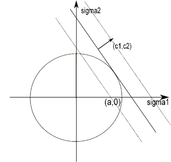
We can get the optimal solution by analyzing the problem geometrically with the norm vector (c1,c2)Tsuperscriptsubscript𝑐1subscript𝑐2𝑇(c_{1},c_{2})^{T} of the objective function as shown in the Fig. 1. The constraint of the problem is represented by the circle with a radius of a𝑎a. We move the line l1subscript𝑙1l_{1} with the slope c1c2subscript𝑐1subscript𝑐2-\dfrac{c_{1}}{c_{2}} to get the largest intercept between l1subscript𝑙1l_{1} and σ2subscript𝜎2\sigma_{2} axis under the constraint that there is an intersection between the circle and the line l1subscript𝑙1l_{1}. The corresponding optimal solution is found when l1subscript𝑙1l_{1} becomes a tangent line to the circle, which is

σ1=c1ac12+c22σ2=c2ac12+c22subscript𝜎1subscript𝑐1𝑎subscriptsuperscript𝑐21subscriptsuperscript𝑐22subscript𝜎2subscript𝑐2𝑎subscriptsuperscript𝑐21subscriptsuperscript𝑐22\begin{split}\sigma_{1}=\frac{c_{1}a}{\sqrt{c^{2}_{1}+c^{2}_{2}}}\\ \sigma_{2}=\frac{c_{2}a}{\sqrt{c^{2}_{1}+c^{2}_{2}}}\\ \end{split} (39)
Refer to caption
Figure 1: Geometric solution for systems with two sensors.

For a system with arbitrary number of sensors, we can repeat the same procedure to find the optimal solution by using hyperplanes and hyperspheres. In general, the optimal attack strategy can be found and summarized as follows.

Theorem 1.

For a system with M𝑀M sensors, the optimal strategy for the adversary is to inject dependent random noises with a pairwise correlation coefficient of 111. The random bias power is allocated such that

σbi=ciaj=1Mcj2,fori=1,,M.formulae-sequencesubscript𝜎subscript𝑏𝑖subscript𝑐𝑖𝑎superscriptsubscript𝑗1𝑀subscriptsuperscript𝑐2𝑗for𝑖1𝑀\sigma_{b_{i}}=\frac{c_{i}a}{\sqrt{\sum_{j=1}^{M}c^{2}_{j}}},\;\;\;\mathrm{for}\;i=1,\cdots,M. (40)

VI-A2 Attack Strategy For A Single Position And Velocity Sensor

In this case, let us assume that the sensors collect both position and velocity measurements of the target. Therefore, the measurement matrix for the i𝑖ith sensor is 𝐇i=𝐈2subscript𝐇𝑖subscript𝐈2{\bf H}_{i}={\bf I}_{2}, where 𝐈2subscript𝐈2{\bf I}_{2} is a 2×2222\times 2 identity matrix. At the i𝑖ith sensor, the adversary injects the bias noise vector 𝐛kisubscript𝐛subscript𝑘𝑖\mathbf{b}_{k_{i}} to the sensor measurement 𝐳kisubscript𝐳subscript𝑘𝑖{\bf z}_{k_{i}}, where 𝐛ki=[bpibvi]Tsubscript𝐛subscript𝑘𝑖superscriptdelimited-[]subscript𝑏subscript𝑝𝑖subscript𝑏subscript𝑣𝑖𝑇\mathbf{b}_{k_{i}}=[b_{p_{i}}\;\;b_{v_{i}}]^{T} consists biases in position and velocity measurements. Let us assume that the system bias vector 𝐛k=[𝐛k1T,,𝐛kMT]Tsubscript𝐛𝑘superscriptsuperscriptsubscript𝐛𝑘1𝑇superscriptsubscript𝐛𝑘𝑀𝑇𝑇{\bf b}_{k}=[{\bf b}_{k1}^{T},\cdots,{\bf b}_{kM}^{T}]^{T} is zero-mean and has a 2M×2M2𝑀2𝑀2M\times 2M covariance matrix 𝚺Ksubscript𝚺𝐾{\bf\Sigma}_{K}. Further, the (i,j)𝑖𝑗(i,\;j)th 2×2222\times 2 submatrix for 𝚺Ksubscript𝚺𝐾{\bf\Sigma}_{K} is defined as

𝚺K(i,j)=[ρbpi,bpjσbpiσbpjρbpi,bvjσbpiσbvjρbvi,bpjσbviσbpjρbvi,bvjσbviσbvj]subscript𝚺𝐾𝑖𝑗delimited-[]subscript𝜌subscriptsubscript𝑏𝑝𝑖subscriptsubscript𝑏𝑝𝑗subscript𝜎subscript𝑏subscript𝑝𝑖subscript𝜎subscript𝑏subscript𝑝𝑗subscript𝜌subscriptsubscript𝑏𝑝𝑖subscriptsubscript𝑏𝑣𝑗subscript𝜎subscriptsubscript𝑏𝑝𝑖subscript𝜎subscriptsubscript𝑏𝑣𝑗missing-subexpressionmissing-subexpressionsubscript𝜌subscriptsubscript𝑏𝑣𝑖subscriptsubscript𝑏𝑝𝑗subscript𝜎subscriptsubscript𝑏𝑣𝑖subscript𝜎subscript𝑏subscript𝑝𝑗subscript𝜌subscriptsubscript𝑏𝑣𝑖subscriptsubscript𝑏𝑣𝑗subscript𝜎subscriptsubscript𝑏𝑣𝑖subscript𝜎subscript𝑏subscript𝑣𝑗missing-subexpressionmissing-subexpression{\bf\Sigma}_{K}(i,j)=\left[\begin{array}[]{cccc}\rho_{{b_{p}}_{i},{b_{p}}_{j}}\sigma_{b_{p_{i}}}\sigma_{b_{p_{j}}}&\rho_{{b_{p}}_{i},{b_{v}}_{j}}\sigma_{{b_{p}}_{i}}\sigma_{{b_{v}}_{j}}\\ \rho_{{b_{v}}_{i},{b_{p}}_{j}}\sigma_{{b_{v}}_{i}}\sigma_{b_{p_{j}}}&\rho_{{b_{v}}_{i},{b_{v}}_{j}}\sigma_{{b_{v}}_{i}}\sigma_{b_{v_{j}}}\\ \end{array}\right] (41)

for 1i,jMformulae-sequence1𝑖𝑗𝑀1\leq i,\;j\leq M. σbpisubscript𝜎subscriptsubscript𝑏𝑝𝑖\sigma_{{b_{p}}_{i}} and σbvisubscript𝜎subscriptsubscript𝑏𝑣𝑖\sigma_{{b_{v}}_{i}} are the position and velocity bias noise standard deviations at the i𝑖ith sensor respectively. The ρ𝜌\rhos are defined as the proper correlation coefficients between components of the bias vector, and ρbpi,bpi=ρbvi,bvi=1subscript𝜌subscriptsubscript𝑏𝑝𝑖subscriptsubscript𝑏𝑝𝑖subscript𝜌subscriptsubscript𝑏𝑣𝑖subscriptsubscript𝑏𝑣𝑖1\rho_{{b_{p}}_{i},{b_{p}}_{i}}=\rho_{{b_{v}}_{i},{b_{v}}_{i}}=1, for 1iM1𝑖𝑀1\leq i\leq M. Since the position bias bpsubscript𝑏𝑝b_{p} and velocity bias bvsubscript𝑏𝑣b_{v} have different units, we need an appropriate constraint for bias noise power. Here we assume that the total noise power is defined as

i=1Mσbpi2+T2σbvi2superscriptsubscript𝑖1𝑀superscriptsubscript𝜎subscript𝑏subscript𝑝𝑖2superscript𝑇2superscriptsubscript𝜎subscript𝑏subscript𝑣𝑖2\sum_{i=1}^{M}\sigma_{b_{p_{i}}}^{2}+T^{2}\sigma_{b_{v_{i}}}^{2} (42)

Note that this is a meaningful power definition, since the two terms in the above equation has the same unit. Recall that according to the target tracking system plant equation and ignoring the system process noise, we have ξk+1=ξk+Tξ˙ksubscript𝜉𝑘1subscript𝜉𝑘𝑇subscript˙𝜉𝑘\xi_{k+1}=\xi_{k}+T\dot{\xi}_{k}. Therefore, the power defined in (42) can be interpreted as the summation of the extra mean squared errors for the position estimate caused by independent bias injections. We can see that the best attack strategy derived under a constraint on power defined in (42) can be easily adjusted and extended for other power definitions, as long as in the new definition, the second term is proportional to T2σbvi2superscript𝑇2superscriptsubscript𝜎subscript𝑏subscript𝑣𝑖2T^{2}\sigma_{b_{v_{i}}}^{2}.

As we can use the equivalent sensor to represent the multiple sensors, we focus on the single-sensor case first. If we are interested in the case of N=0𝑁0N=0, maximizing the trace of 𝐀Ksubscript𝐀𝐾{\bf A}_{K} is equivalent to maximize the 𝐖K𝚺K𝐖KTsubscript𝐖𝐾subscript𝚺𝐾subscriptsuperscript𝐖𝑇𝐾\mathbf{W}_{K}{\bf\Sigma}_{K}\mathbf{W}^{T}_{K}. We assume that the adversary knows the system models and the prior information 𝐏0|0subscript𝐏conditional00{\bf P}_{0|0} at time zero, so that he/she can calculate the offline Kalman filter gain matrix 𝐖ksubscript𝐖𝑘{\bf W}_{k} recursively. Therefore, the best strategy the adversary can adopt to attack the system is the solution to the following optimization problem:

max𝚺KTr[𝐖K𝚺K𝐖KT]subscriptsubscript𝚺𝐾Trdelimited-[]subscript𝐖𝐾subscript𝚺𝐾subscriptsuperscript𝐖𝑇𝐾\displaystyle\max_{{\bf\Sigma}_{K}}\mathrm{Tr}\left[\mathbf{W}_{K}{\bf\Sigma}_{K}\mathbf{W}^{T}_{K}\right]
s.t.σbp2+T2σbv2=a2formulae-sequence𝑠𝑡superscriptsubscript𝜎subscript𝑏𝑝2superscript𝑇2superscriptsubscript𝜎subscript𝑏𝑣2superscript𝑎2\displaystyle s.t.\;\;\;\sigma_{b_{p}}^{2}+T^{2}\sigma_{b_{v}}^{2}=a^{2}
1ρbp,bv11subscript𝜌subscript𝑏𝑝subscript𝑏𝑣1\displaystyle\;\;\;\;\;\ -1\leq\rho_{b_{p},b_{v}}\leq 1
σbp,σbv>0subscript𝜎subscript𝑏𝑝subscript𝜎subscript𝑏𝑣0\displaystyle\;\;\;\;\;\ \sigma_{b_{p}},\sigma_{b_{v}}>0 (43)

where

𝚺K=[σbp2ρbp,bvσbpσbvρbp,bvσbpσbvσbv2]subscript𝚺𝐾delimited-[]superscriptsubscript𝜎subscript𝑏𝑝2subscript𝜌subscript𝑏𝑝subscript𝑏𝑣subscript𝜎subscript𝑏𝑝subscript𝜎subscript𝑏𝑣subscript𝜌subscript𝑏𝑝subscript𝑏𝑣subscript𝜎subscript𝑏𝑝subscript𝜎subscript𝑏𝑣superscriptsubscript𝜎subscript𝑏𝑣2\boldsymbol{\Sigma}_{K}=\left[\begin{array}[]{cc}\sigma_{b_{p}}^{2}&\rho_{b_{p},b_{v}}\sigma_{b_{p}}\sigma_{b_{v}}\\ \rho_{b_{p},b_{v}}\sigma_{b_{p}}\sigma_{b_{v}}&\sigma_{b_{v}}^{2}\\ \end{array}\right] (44)

and

𝐖K=[w11w12w21w22]subscript𝐖𝐾delimited-[]subscript𝑤11subscript𝑤12subscript𝑤21subscript𝑤22\mathbf{W}_{K}=\left[\begin{array}[]{cc}w_{11}&w_{12}\\ w_{21}&w_{22}\\ \end{array}\right] (45)

It is easy to show that

Tr[𝐖K𝚺K𝐖KT]=Tr[𝐖KT𝐖K𝚺K]=(w112+w212)σbp2+(w122+w222)σbv2+2(w11w12+w21w22)ρbp,bvσbpσbvTrdelimited-[]subscript𝐖𝐾subscript𝚺𝐾subscriptsuperscript𝐖𝑇𝐾Trdelimited-[]subscriptsuperscript𝐖𝑇𝐾subscript𝐖𝐾subscript𝚺𝐾superscriptsubscript𝑤112superscriptsubscript𝑤212superscriptsubscript𝜎subscript𝑏𝑝2superscriptsubscript𝑤122superscriptsubscript𝑤222superscriptsubscript𝜎subscript𝑏𝑣22subscript𝑤11subscript𝑤12subscript𝑤21subscript𝑤22subscript𝜌subscript𝑏𝑝subscript𝑏𝑣subscript𝜎subscript𝑏𝑝subscript𝜎subscript𝑏𝑣\displaystyle\begin{split}\mathrm{Tr}&\left[\mathbf{W}_{K}{\bf\Sigma}_{K}\mathbf{W}^{T}_{K}\right]=\mathrm{Tr}\left[\mathbf{W}^{T}_{K}\mathbf{W}_{K}{\bf\Sigma}_{K}\right]\\ &=(w_{11}^{2}+w_{21}^{2})\sigma_{b_{p}}^{2}+(w_{12}^{2}+w_{22}^{2})\sigma_{b_{v}}^{2}\\ &+2(w_{11}w_{12}+w_{21}w_{22})\rho_{b_{p},b_{v}}\sigma_{b_{p}}\sigma_{b_{v}}\\ \end{split} (46)

According to the sign of (w11w12+w21w22)subscript𝑤11subscript𝑤12subscript𝑤21subscript𝑤22(w_{11}w_{12}+w_{21}w_{22}), we can set the value of the ρbp,bvsubscript𝜌subscript𝑏𝑝subscript𝑏𝑣\rho_{b_{p},b_{v}} to maximize the objective function. For example, if (w11w12+w21w22)subscript𝑤11subscript𝑤12subscript𝑤21subscript𝑤22(w_{11}w_{12}+w_{21}w_{22}) is positive, we set ρbp,bv=1subscript𝜌subscript𝑏𝑝subscript𝑏𝑣1\rho_{b_{p},b_{v}}=1 and the optimization problem becomes

max(w11σbp+w12σbv)2+(w21σbp+w22σbv)2\displaystyle\max(w_{11}\sigma_{b_{p}}+w_{12}\sigma_{b_{v}})^{2}+(w_{21}\sigma_{b_{p}}+w_{22}\sigma_{b_{v}})^{2}
s.t.σbp2+T2σbv2=a2formulae-sequence𝑠𝑡superscriptsubscript𝜎subscript𝑏𝑝2superscript𝑇2superscriptsubscript𝜎subscript𝑏𝑣2superscript𝑎2\displaystyle s.t.\;\;\;\sigma_{b_{p}}^{2}+T^{2}\sigma_{b_{v}}^{2}=a^{2} (47)
σbp,σbv0subscript𝜎subscript𝑏𝑝subscript𝜎subscript𝑏𝑣0\displaystyle\;\;\;\sigma_{b_{p}},\sigma_{b_{v}}\geq 0

To solve this constrained optimization problem, let us first denote

w112+w212=β1w122+w222=β2w11w12=α1w21w22=α2superscriptsubscript𝑤112superscriptsubscript𝑤212subscript𝛽1superscriptsubscript𝑤122superscriptsubscript𝑤222subscript𝛽2subscript𝑤11subscript𝑤12subscript𝛼1subscript𝑤21subscript𝑤22subscript𝛼2\displaystyle\begin{split}w_{11}^{2}+w_{21}^{2}=\beta_{1}\\ w_{12}^{2}+w_{22}^{2}=\beta_{2}\\ w_{11}w_{12}=\alpha_{1}\\ w_{21}w_{22}=\alpha_{2}\\ \end{split} (48)

The constraint in (43) can be written as

σbp2T2+σbv2=a2T2=a12superscriptsubscript𝜎subscript𝑏𝑝2superscript𝑇2superscriptsubscript𝜎subscript𝑏𝑣2superscript𝑎2superscript𝑇2superscriptsubscript𝑎12\displaystyle\frac{\sigma_{b_{p}}^{2}}{T^{2}}+\sigma_{b_{v}}^{2}=\frac{a^{2}}{T^{2}}=a_{1}^{2} (49)

Now we set σbp=a1Tsin(θ)subscript𝜎subscript𝑏𝑝subscript𝑎1𝑇𝜃\sigma_{b_{p}}=a_{1}T\sin(\theta) and σbv=a1cos(θ)subscript𝜎subscript𝑏𝑣subscript𝑎1𝜃\sigma_{b_{v}}=a_{1}\cos(\theta). Plugging σbpsubscript𝜎subscript𝑏𝑝\sigma_{b_{p}} and σbvsubscript𝜎subscript𝑏𝑣\sigma_{b_{v}} into the objective function, we have the following equivalent optimization problem

maxθa12[β1T12+β22+Asin(2θ+ϕ)]subscript𝜃superscriptsubscript𝑎12delimited-[]subscript𝛽1superscriptsubscript𝑇12subscript𝛽22𝐴2𝜃italic-ϕ\displaystyle\max_{\theta}a_{1}^{2}\left[\frac{\beta_{1}T_{1}^{2}+\beta_{2}}{2}+A\sin(2\theta+\phi)\right]
s.t.   0θπ2formulae-sequence𝑠𝑡.0𝜃𝜋2\displaystyle s.t.\;\;\;0\leq\theta\leq\frac{\pi}{2} (50)

where

A𝐴\displaystyle A =\displaystyle= 14(β2β1T2)2+T2(α1+α2)214superscriptsubscript𝛽2subscript𝛽1superscript𝑇22superscript𝑇2superscriptsubscript𝛼1subscript𝛼22\displaystyle\sqrt{\frac{1}{4}\left(\beta_{2}-\beta_{1}T^{2}\right)^{2}+T^{2}(\alpha_{1}+\alpha_{2})^{2}} (51)
tan(ϕ)italic-ϕ\displaystyle\tan(\phi) =\displaystyle= β2β1T22T(α1+α2)subscript𝛽2subscript𝛽1superscript𝑇22𝑇subscript𝛼1subscript𝛼2\displaystyle\frac{\beta_{2}-\beta_{1}T^{2}}{2T(\alpha_{1}+\alpha_{2})} (52)

Clearly, the optimal solution is

θ=π4ϕ2superscript𝜃𝜋4italic-ϕ2\theta^{*}=\frac{\pi}{4}-\frac{\phi}{2} (53)

We summarize this result in the following theorem.

Theorem 2.

For a system with one sensor observing position and velocity of the target, the optimal strategy for the adversary is to inject random noise that has dependent position and velocity components. If w11w12+w21w22>0subscript𝑤11subscript𝑤12subscript𝑤21subscript𝑤220w_{11}w_{12}+w_{21}w_{22}>0, the correlation coefficient ρbp,bvsubscript𝜌subscript𝑏𝑝subscript𝑏𝑣\rho_{b_{p},b_{v}} should be set as 111, and the random bias power is allocated such that

σbp=asin(θ)subscript𝜎subscript𝑏𝑝𝑎superscript𝜃\displaystyle\sigma_{b_{p}}=a\sin(\theta^{*}) (54)
σbv=aTcos(θ)subscript𝜎subscript𝑏𝑣𝑎𝑇superscript𝜃\displaystyle\sigma_{b_{v}}=\frac{a}{T}\cos(\theta^{*})
θ=π4ϕ2superscript𝜃𝜋4italic-ϕ2\displaystyle\theta^{*}=\frac{\pi}{4}-\frac{\phi}{2}
ϕ=arctan[β2β1T22T(α1+α2)]italic-ϕsubscript𝛽2subscript𝛽1superscript𝑇22𝑇subscript𝛼1subscript𝛼2\displaystyle\phi=\arctan\left[\frac{\beta_{2}-\beta_{1}T^{2}}{2T(\alpha_{1}+\alpha_{2})}\right]
w112+w212=β1superscriptsubscript𝑤112superscriptsubscript𝑤212subscript𝛽1\displaystyle w_{11}^{2}+w_{21}^{2}=\beta_{1}
w122+w222=β2superscriptsubscript𝑤122superscriptsubscript𝑤222subscript𝛽2\displaystyle w_{12}^{2}+w_{22}^{2}=\beta_{2}
w11w12=α1subscript𝑤11subscript𝑤12subscript𝛼1\displaystyle w_{11}w_{12}=\alpha_{1}
w21w22=α2subscript𝑤21subscript𝑤22subscript𝛼2\displaystyle w_{21}w_{22}=\alpha_{2}

When w11w12+w21w22<0subscript𝑤11subscript𝑤12subscript𝑤21subscript𝑤220w_{11}w_{12}+w_{21}w_{22}<0, we should set ρbp,bv=1subscript𝜌subscript𝑏𝑝subscript𝑏𝑣1\rho_{b_{p},b_{v}}=-1 and set α1=w11w12subscript𝛼1subscript𝑤11subscript𝑤12\alpha_{1}=-w_{11}w_{12} and α2=w21w22subscript𝛼2subscript𝑤21subscript𝑤22\alpha_{2}=-w_{21}w_{22}. The rest of the equations in formula (54) remains the same.

VI-A3 Attack Strategy For Multiple Position And Velocity Senors

In this case, M=2𝑀2M=2, and the measurement matrix is 𝐇=[𝐈2𝐈2]T𝐇superscriptdelimited-[]subscript𝐈2subscript𝐈2𝑇{\bf H}=[{\bf I}_{2}\;{\bf I}_{2}]^{T}. The measurement covariance matrix for the i𝑖ith sensor is assumed to be

𝐑i=[σpi200σvi2]subscript𝐑𝑖delimited-[]subscriptsuperscript𝜎2subscript𝑝𝑖0missing-subexpression0subscriptsuperscript𝜎2subscript𝑣𝑖missing-subexpression{\bf R}_{i}=\left[\begin{array}[]{ccc}\sigma^{2}_{p_{i}}&0\\ 0&\sigma^{2}_{v_{i}}\\ \end{array}\right] (55)

Now, according to (25), we have

𝐑e=[𝐑11+𝐑21]1=[(σp12+σp22)100(σv12+σv22)1]subscript𝐑𝑒superscriptdelimited-[]subscriptsuperscript𝐑11subscriptsuperscript𝐑121delimited-[]superscriptsubscriptsuperscript𝜎2subscript𝑝1subscriptsuperscript𝜎2subscript𝑝2100superscriptsubscriptsuperscript𝜎2subscript𝑣1subscriptsuperscript𝜎2subscript𝑣21\begin{split}{\bf R}_{e}&=[{\bf R}^{-1}_{1}+{\bf R}^{-1}_{2}]^{-1}\\ &=\left[\begin{array}[]{cc}\left(\sigma^{-2}_{p_{1}}+\sigma^{-2}_{p_{2}}\right)^{-1}&0\\ 0&\left(\sigma^{-2}_{v_{1}}+\sigma^{-2}_{v_{2}}\right)^{-1}\\ \end{array}\right]\end{split} (56)

According to (24), we define

𝐂i=𝐑e𝐇iT𝐑i1=[σpi2σp12+σp2200σvi2σv12+σv22]subscript𝐂𝑖subscript𝐑𝑒superscriptsubscript𝐇𝑖𝑇subscriptsuperscript𝐑1𝑖delimited-[]subscriptsuperscript𝜎2subscript𝑝𝑖subscriptsuperscript𝜎2subscript𝑝1subscriptsuperscript𝜎2subscript𝑝20missing-subexpression0subscriptsuperscript𝜎2subscript𝑣𝑖subscriptsuperscript𝜎2subscript𝑣1subscriptsuperscript𝜎2subscript𝑣2missing-subexpression\begin{split}{\bf C}_{i}&={\bf R}_{e}{\bf H}_{i}^{T}{\bf R}^{-1}_{i}\\ &=\left[\begin{array}[]{ccc}\frac{\sigma^{-2}_{p_{i}}}{\sigma^{-2}_{p_{1}}+\sigma^{-2}_{p_{2}}}&0\\ 0&\frac{\sigma^{-2}_{v_{i}}}{\sigma^{-2}_{v_{1}}+\sigma^{-2}_{v_{2}}}\\ \end{array}\right]\end{split} (57)

as the weighting matrix for the i𝑖ith sensor’s observation 𝐳isubscript𝐳𝑖{\bf z}_{i}. Further, we define

cpi=𝐂i(1,1)cvi=𝐂i(2,2)subscript𝑐subscript𝑝𝑖subscript𝐂𝑖11subscript𝑐subscript𝑣𝑖subscript𝐂𝑖22\begin{split}c_{p_{i}}={\bf C}_{i}(1,1)\\ c_{v_{i}}={\bf C}_{i}(2,2)\end{split} (58)

both of which are positive numbers. The equivalent noise injection is therefore

𝐛eK=i=12𝐂i𝐛Kisubscript𝐛𝑒𝐾superscriptsubscript𝑖12subscript𝐂𝑖subscript𝐛subscript𝐾𝑖{\bf b}_{eK}=\sum_{i=1}^{2}{\bf C}_{i}{\bf b}_{K_{i}} (59)

So the covariance matrix of the equivalent bias vector is

𝚺eK=i=12i=j2𝐂i𝚺K(i,j)𝐂jTsubscript𝚺𝑒𝐾superscriptsubscript𝑖12superscriptsubscript𝑖𝑗2subscript𝐂𝑖subscript𝚺𝐾𝑖𝑗superscriptsubscript𝐂𝑗𝑇{\bf\Sigma}_{eK}=\sum_{i=1}^{2}\sum_{i=j}^{2}{\bf C}_{i}{\bf\Sigma}_{K}(i,j){\bf C}_{j}^{T} (60)

where 𝚺K(i,j)subscript𝚺𝐾𝑖𝑗{\bf\Sigma}_{K}(i,j) has been defined in (41). It can be shown that

𝚺eK=[s1s2s2s3]subscript𝚺𝑒𝐾delimited-[]subscript𝑠1subscript𝑠2subscript𝑠2subscript𝑠3{\bf\Sigma}_{eK}=\left[\begin{array}[]{cc}s_{1}&s_{2}\\ s_{2}&s_{3}\\ \end{array}\right] (61)

Where

s1=cp12σbp12+cp22σbp22+2ρbp1,bp2cp1cp2σbp1σbp2s3=cv12σbv12+cv22σbv22+2ρbv1,bv2cv1cv2σbv1σbv2subscript𝑠1superscriptsubscript𝑐subscript𝑝12superscriptsubscript𝜎subscript𝑏subscript𝑝12superscriptsubscript𝑐subscript𝑝22superscriptsubscript𝜎subscript𝑏subscript𝑝222subscript𝜌subscript𝑏subscript𝑝1subscript𝑏subscript𝑝2subscript𝑐subscript𝑝1subscript𝑐subscript𝑝2subscript𝜎subscript𝑏subscript𝑝1subscript𝜎subscript𝑏subscript𝑝2subscript𝑠3superscriptsubscript𝑐subscript𝑣12superscriptsubscript𝜎subscript𝑏subscript𝑣12superscriptsubscript𝑐subscript𝑣22superscriptsubscript𝜎subscript𝑏subscript𝑣222subscript𝜌subscript𝑏subscript𝑣1subscript𝑏subscript𝑣2subscript𝑐subscript𝑣1subscript𝑐subscript𝑣2subscript𝜎subscript𝑏subscript𝑣1subscript𝜎subscript𝑏subscript𝑣2\begin{split}s_{1}=c_{p_{1}}^{2}\sigma_{b_{p_{1}}}^{2}+c_{p_{2}}^{2}\sigma_{b_{p_{2}}}^{2}+2\rho_{b_{p_{1}},b_{p_{2}}}c_{p_{1}}c_{p_{2}}\sigma_{b_{p_{1}}}\sigma_{b_{p_{2}}}\\ s_{3}=c_{v_{1}}^{2}\sigma_{b_{v_{1}}}^{2}+c_{v_{2}}^{2}\sigma_{b_{v_{2}}}^{2}+2\rho_{b_{v_{1}},b_{v_{2}}}c_{v_{1}}c_{v_{2}}\sigma_{b_{v_{1}}}\sigma_{b_{v_{2}}}\end{split} (62)
s2=cp1cv1ρbp1,bv1σbp1σbv1+cp1cv2ρbp1,bv2σbp1σbv2+cp2cv1ρbp2,bv1σbp2σbv1+cp2cv2ρbp2,bv2σbp2σbv2subscript𝑠2subscript𝑐subscript𝑝1subscript𝑐subscript𝑣1subscript𝜌subscript𝑏subscript𝑝1subscript𝑏subscript𝑣1subscript𝜎subscript𝑏subscript𝑝1subscript𝜎subscript𝑏subscript𝑣1subscript𝑐subscript𝑝1subscript𝑐subscript𝑣2subscript𝜌subscript𝑏subscript𝑝1subscript𝑏subscript𝑣2subscript𝜎subscript𝑏subscript𝑝1subscript𝜎subscript𝑏subscript𝑣2subscript𝑐subscript𝑝2subscript𝑐subscript𝑣1subscript𝜌subscript𝑏subscript𝑝2subscript𝑏subscript𝑣1subscript𝜎subscript𝑏subscript𝑝2subscript𝜎subscript𝑏subscript𝑣1subscript𝑐subscript𝑝2subscript𝑐subscript𝑣2subscript𝜌subscript𝑏subscript𝑝2subscript𝑏subscript𝑣2subscript𝜎subscript𝑏subscript𝑝2subscript𝜎subscript𝑏subscript𝑣2\begin{split}s_{2}&=c_{p_{1}}c_{v_{1}}\rho_{b_{p_{1}},b_{v_{1}}}\sigma_{b_{p_{1}}}\sigma_{b_{v_{1}}}+c_{p_{1}}c_{v_{2}}\rho_{b_{p_{1}},b_{v_{2}}}\sigma_{b_{p_{1}}}\sigma_{b_{v_{2}}}\\ &+c_{p_{2}}c_{v_{1}}\rho_{b_{p_{2}},b_{v_{1}}}\sigma_{b_{p_{2}}}\sigma_{b_{v_{1}}}+c_{p_{2}}c_{v_{2}}\rho_{b_{p_{2}},b_{v_{2}}}\sigma_{b_{p_{2}}}\sigma_{b_{v_{2}}}\end{split} (63)

The optimization problem can be written as follows.

max𝚺eKTr[𝐖eK𝚺eK𝐖eKT]subscriptsubscript𝚺𝑒𝐾Trdelimited-[]subscript𝐖𝑒𝐾subscript𝚺𝑒𝐾subscriptsuperscript𝐖𝑇𝑒𝐾\displaystyle\max_{{\bf\Sigma}_{eK}}\mathrm{Tr}\left[\mathbf{W}_{eK}{\bf\Sigma}_{eK}\mathbf{W}^{T}_{eK}\right] (64)
s.t.σbp12+σbp22+T2σbv12+T2σbv22=a2,formulae-sequence𝑠𝑡superscriptsubscript𝜎subscript𝑏subscript𝑝12superscriptsubscript𝜎subscript𝑏subscript𝑝22superscript𝑇2superscriptsubscript𝜎subscript𝑏subscript𝑣12superscript𝑇2superscriptsubscript𝜎subscript𝑏subscript𝑣22superscript𝑎2\displaystyle s.t.\;\;\;\sigma_{b_{p_{1}}}^{2}+\sigma_{b_{p_{2}}}^{2}+T^{2}\sigma_{b_{v_{1}}}^{2}+T^{2}\sigma_{b_{v_{2}}}^{2}=a^{2},
1ρpi,vj1,1subscript𝜌subscript𝑝𝑖subscript𝑣𝑗1\displaystyle\;\;\;\;\;\ -1\leq\rho_{p_{i},v_{j}}\leq 1,
1ρvi,vj1,1subscript𝜌subscript𝑣𝑖subscript𝑣𝑗1\displaystyle\;\;\;\;\;\ -1\leq\rho_{v_{i},v_{j}}\leq 1,
1ρpi,pj1,1subscript𝜌subscript𝑝𝑖subscript𝑝𝑗1\displaystyle\;\;\;\;\;\ -1\leq\rho_{p_{i},p_{j}}\leq 1,
σpi,σvi0,i,j{1,2}formulae-sequencesubscript𝜎subscript𝑝𝑖subscript𝜎subscript𝑣𝑖0for-all𝑖𝑗12\displaystyle\;\;\;\;\;\ \sigma_{p_{i}},\sigma_{v_{i}}\geq 0,\;\;\;\forall i,j\in\{1,2\}

where

𝐖eK=[w11w12w21w22]subscript𝐖𝑒𝐾delimited-[]subscript𝑤11subscript𝑤12subscript𝑤21subscript𝑤22\mathbf{W}_{eK}=\left[\begin{array}[]{cc}w_{11}&w_{12}\\ w_{21}&w_{22}\\ \end{array}\right] (65)

is Kalman filter gain calculated using the equivalent measurement covariance matrix 𝐑esubscript𝐑𝑒{\bf R}_{e} and equivalent measurement matrix 𝐇esubscript𝐇𝑒{\bf H}_{e}. It is easy to show that

Tr[𝐖K𝚺K𝐖KT]=Tr[𝐖KT𝐖K𝚺K]Trdelimited-[]subscript𝐖𝐾subscript𝚺𝐾subscriptsuperscript𝐖𝑇𝐾Trdelimited-[]subscriptsuperscript𝐖𝑇𝐾subscript𝐖𝐾subscript𝚺𝐾\displaystyle\mathrm{Tr}\left[\mathbf{W}_{K}{\bf\Sigma}_{K}\mathbf{W}^{T}_{K}\right]=\mathrm{Tr}\left[\mathbf{W}^{T}_{K}\mathbf{W}_{K}{\bf\Sigma}_{K}\right] (66)
=(w112+w212)2s1+(w122+w222)2s3absentsuperscriptsubscriptsuperscript𝑤211subscriptsuperscript𝑤2212subscript𝑠1superscriptsubscriptsuperscript𝑤212subscriptsuperscript𝑤2222subscript𝑠3\displaystyle=(w^{2}_{11}+w^{2}_{21})^{2}s_{1}+(w^{2}_{12}+w^{2}_{22})^{2}s_{3}
+2(w11w12+w21w22)s22subscript𝑤11subscript𝑤12subscript𝑤21subscript𝑤22subscript𝑠2\displaystyle+2(w_{11}w_{12}+w_{21}w_{22})s_{2}

Clearly, all the ρ𝜌\rhos that appear in s1subscript𝑠1s_{1} and s3subscript𝑠3s_{3} should be set as 1 to maximize the objective function. The optimal values for ρ𝜌\rhos in s2subscript𝑠2s_{2} depend on Kalman filter gain 𝐖eKsubscript𝐖𝑒𝐾{\bf W}_{eK}. More specifically, when w11w12+w21w22>0subscript𝑤11subscript𝑤12subscript𝑤21subscript𝑤220w_{11}w_{12}+w_{21}w_{22}>0, all the ρ𝜌\rhos that appear in s2subscript𝑠2s_{2} should be set to 111; otherwise, they should be set as 11-1. Let us first suppose that w11w12+w21w22>0subscript𝑤11subscript𝑤12subscript𝑤21subscript𝑤220w_{11}w_{12}+w_{21}w_{22}>0 is true, then we have

Tr[𝐖K𝚺K𝐖KT]=(w112+w212)2(cp1σp1+cp2σp2)2+(w122+w222)2(cv1σv1+cv2σv2)2+2(w11w12+w21w22)(cp1cv1σp1σv1+cp1cv2σp1σv2+cp2cv1σp2σv1+cp2cv2σp2σv2)Trdelimited-[]subscript𝐖𝐾subscript𝚺𝐾subscriptsuperscript𝐖𝑇𝐾superscriptsubscriptsuperscript𝑤211subscriptsuperscript𝑤2212superscriptsubscript𝑐subscript𝑝1subscript𝜎subscript𝑝1subscript𝑐subscript𝑝2subscript𝜎subscript𝑝22superscriptsubscriptsuperscript𝑤212subscriptsuperscript𝑤2222superscriptsubscript𝑐subscript𝑣1subscript𝜎subscript𝑣1subscript𝑐subscript𝑣2subscript𝜎subscript𝑣222subscript𝑤11subscript𝑤12subscript𝑤21subscript𝑤22subscript𝑐subscript𝑝1subscript𝑐subscript𝑣1subscript𝜎subscript𝑝1subscript𝜎subscript𝑣1subscript𝑐subscript𝑝1subscript𝑐subscript𝑣2subscript𝜎subscript𝑝1subscript𝜎subscript𝑣2subscript𝑐subscript𝑝2subscript𝑐subscript𝑣1subscript𝜎subscript𝑝2subscript𝜎subscript𝑣1subscript𝑐subscript𝑝2subscript𝑐subscript𝑣2subscript𝜎subscript𝑝2subscript𝜎subscript𝑣2\displaystyle\begin{split}&\mathrm{Tr}\left[\mathbf{W}_{K}{\bf\Sigma}_{K}\mathbf{W}^{T}_{K}\right]=(w^{2}_{11}+w^{2}_{21})^{2}(c_{p_{1}}\sigma_{p_{1}}+c_{p_{2}}\sigma_{p_{2}})^{2}\\ &+(w^{2}_{12}+w^{2}_{22})^{2}(c_{v_{1}}\sigma_{v_{1}}+c_{v_{2}}\sigma_{v_{2}})^{2}\\ &+2(w_{11}w_{12}+w_{21}w_{22})(c_{p_{1}}c_{v_{1}}\sigma_{p_{1}}\sigma_{v_{1}}+c_{p_{1}}c_{v_{2}}\sigma_{p_{1}}\sigma_{v_{2}}\\ &+c_{p_{2}}c_{v_{1}}\sigma_{p_{2}}\sigma_{v_{1}}+c_{p_{2}}c_{v_{2}}\sigma_{p_{2}}\sigma_{v_{2}})\end{split} (67)

So far, we have converted the objective function in (64), which involves 10 variables to one that involves only 4 variables. Considering that the power constraint reduces one degree of freedom, we only need to solve an optimization problem in a 3-dimensional space.

VI-A4 Strategy For A Single Sensor With Multiple Time Attack

Based on Proposition 2, we get the extra mean square matrix,

𝐀K+N=m=0N𝐃m𝚺K+Nm𝐃mTsubscript𝐀𝐾𝑁superscriptsubscript𝑚0𝑁subscript𝐃𝑚subscript𝚺𝐾𝑁𝑚subscriptsuperscript𝐃𝑇𝑚\displaystyle\mathbf{A}_{K+N}=\sum_{m=0}^{N}\mathbf{D}_{m}{\bf\Sigma}_{K+N-m}\mathbf{D}^{T}_{m}

Suppose at the time K𝐾K, the adversary wants to attack the system continuously from time K𝐾K to K+N𝐾𝑁K+N, the weight for different time is αi,iNsubscript𝛼𝑖𝑖𝑁\alpha_{i},i\in N, as shown below,

𝐀K+0=α0(𝐃0𝚺K𝐃0T)subscriptsuperscript𝐀𝐾0subscript𝛼0subscript𝐃0subscript𝚺𝐾subscriptsuperscript𝐃𝑇0\displaystyle\mathbf{A}^{{}^{\prime}}_{K+0}=\alpha_{0}(\mathbf{D}_{0}{\bf\Sigma}_{K}\mathbf{D}^{T}_{0})
𝐀K+1=α1(𝐃0𝚺K+1𝐃0T+𝐃1𝚺K𝐃1T)subscriptsuperscript𝐀𝐾1subscript𝛼1subscript𝐃0subscript𝚺𝐾1subscriptsuperscript𝐃𝑇0subscript𝐃1subscript𝚺𝐾subscriptsuperscript𝐃𝑇1\displaystyle\mathbf{A}^{{}^{\prime}}_{K+1}=\alpha_{1}(\mathbf{D}_{0}{\bf\Sigma}_{K+1}\mathbf{D}^{T}_{0}+\mathbf{D}_{1}{\bf\Sigma}_{K}\mathbf{D}^{T}_{1}) (68)
\displaystyle...
𝐀K+N=αN(𝐃0𝚺K+N𝐃0T++𝐃N𝚺K𝐃NT)subscriptsuperscript𝐀𝐾𝑁subscript𝛼𝑁subscript𝐃0subscript𝚺𝐾𝑁subscriptsuperscript𝐃𝑇0subscript𝐃𝑁subscript𝚺𝐾subscriptsuperscript𝐃𝑇𝑁\displaystyle\mathbf{A}^{{}^{\prime}}_{K+N}=\alpha_{N}(\mathbf{D}_{0}{\bf\Sigma}_{K+N}\mathbf{D}^{T}_{0}+...+\mathbf{D}_{N}{\bf\Sigma}_{K}\mathbf{D}^{T}_{N})

where m=0Nαm=1subscriptsuperscript𝑁𝑚0subscript𝛼𝑚1\sum^{N}_{m=0}\alpha_{m}=1. So the objective function in the multi-shot attack case is the trace of the weighted sum of the EMSE matrices at different time points that is m=0Nαm𝐀K+m=m=0N𝐀K+msuperscriptsubscript𝑚0𝑁subscript𝛼𝑚subscript𝐀𝐾𝑚superscriptsubscript𝑚0𝑁subscriptsuperscript𝐀𝐾𝑚\sum_{m=0}^{N}\alpha_{m}\mathbf{A}_{K+m}=\sum_{m=0}^{N}\mathbf{A}^{{}^{\prime}}_{K+m}. It is equivalent to maximize the trace of the weighted sum of the MSE matrices of the state estimates, because once the system reaches its steady state, 𝐏K+m|K+msubscript𝐏𝐾conditional𝑚𝐾𝑚{\bf P}_{K+m|K+m} becomes constant, and the weighted sum of 𝐏K+m|K+msubscript𝐏𝐾conditional𝑚𝐾𝑚{\bf P}_{K+m|K+m} will remain the same. First we study the case where the system has position sensors which are being attacked, so all the items above are scalars. Using lower case d,σp2𝑑superscriptsubscript𝜎𝑝2d,\sigma_{p}^{2} to denote 𝐃,𝚺𝐃𝚺\mathbf{D},{\bf\Sigma}, we can formulate the optimization problem below,

maxσpK,,σpK+Nsubscriptsubscript𝜎subscript𝑝𝐾subscript𝜎subscript𝑝𝐾𝑁\displaystyle\max_{\sigma_{p_{K}},\cdots,\sigma_{p_{K+N}}} m=0Nαm𝐀K+m=m=0N𝐀K+msuperscriptsubscript𝑚0𝑁subscript𝛼𝑚subscript𝐀𝐾𝑚superscriptsubscript𝑚0𝑁subscriptsuperscript𝐀𝐾𝑚\displaystyle\sum_{m=0}^{N}\alpha_{m}\mathbf{A}_{K+m}=\sum_{m=0}^{N}\mathbf{A}^{{}^{\prime}}_{K+m}
=σpK2(α0d02+α1d12++αNdN2)absentsubscriptsuperscript𝜎2subscript𝑝𝐾subscript𝛼0subscriptsuperscript𝑑20subscript𝛼1subscriptsuperscript𝑑21subscript𝛼𝑁subscriptsuperscript𝑑2𝑁\displaystyle=\sigma^{2}_{p_{K}}(\alpha_{0}d^{2}_{0}+\alpha_{1}d^{2}_{1}+...+\alpha_{N}d^{2}_{N})
+σpK+12(α1d02+α2d12++αNdN12)subscriptsuperscript𝜎2subscript𝑝𝐾1subscript𝛼1subscriptsuperscript𝑑20subscript𝛼2subscriptsuperscript𝑑21subscript𝛼𝑁subscriptsuperscript𝑑2𝑁1\displaystyle+\sigma^{2}_{p_{K+1}}(\alpha_{1}d^{2}_{0}+\alpha_{2}d^{2}_{1}+...+\alpha_{N}d^{2}_{N-1})
+σpK+22(α2d02+α3d12++αNdN22)subscriptsuperscript𝜎2subscript𝑝𝐾2subscript𝛼2subscriptsuperscript𝑑20subscript𝛼3subscriptsuperscript𝑑21subscript𝛼𝑁subscriptsuperscript𝑑2𝑁2\displaystyle+\sigma^{2}_{p_{K+2}}(\alpha_{2}d^{2}_{0}+\alpha_{3}d^{2}_{1}+...+\alpha_{N}d^{2}_{N-2})
+\displaystyle+...
+σpK+N2(αNd02)subscriptsuperscript𝜎2subscript𝑝𝐾𝑁subscript𝛼𝑁subscriptsuperscript𝑑20\displaystyle+\sigma^{2}_{p_{K+N}}(\alpha_{N}d^{2}_{0})
s.t.formulae-sequence𝑠𝑡\displaystyle s.t. m=KK+Nσpm2a2superscriptsubscript𝑚𝐾𝐾𝑁subscriptsuperscript𝜎2subscript𝑝𝑚superscript𝑎2\displaystyle\sum_{m=K}^{K+N}\sigma^{2}_{p_{m}}\leq a^{2}
m=0Nαm=1subscriptsuperscript𝑁𝑚0subscript𝛼𝑚1\displaystyle\sum^{N}_{m=0}\alpha_{m}=1

The adversary can allocate the power based on the coefficients of the variance variables at different time. For example, if the weights αmssuperscriptsubscript𝛼𝑚𝑠\alpha_{m}^{\prime}s are all the same, the best strategy is to allocate all the power to the sensors at the first beginning (at time K) because the coefficient for σpK2subscriptsuperscript𝜎2subscript𝑝𝐾\sigma^{2}_{p_{K}} is the largest. Second, if the sensors measure both position and velocity, and the attacker aims to attack the system with position and velocity false information, the optimization problem can be characterized as below,

max𝚺K,,𝚺K+Nsubscriptsubscript𝚺𝐾subscript𝚺𝐾𝑁\displaystyle\max_{\boldsymbol{\Sigma}_{K},\cdots,\boldsymbol{\Sigma}_{K+N}} Tr[m=0Nαm𝐀K+m]=Tr[m=0N𝐀K+m]Trdelimited-[]superscriptsubscript𝑚0𝑁subscript𝛼𝑚subscript𝐀𝐾𝑚Trdelimited-[]superscriptsubscript𝑚0𝑁subscriptsuperscript𝐀𝐾𝑚\displaystyle\mathrm{Tr}\left[\sum_{m=0}^{N}\alpha_{m}\mathbf{A}_{K+m}\right]=\mathrm{Tr}\left[\sum_{m=0}^{N}\mathbf{A}^{{}^{\prime}}_{K+m}\right]
=Tr[𝚺K(α0𝐃0T𝐃0++αN𝐃NT𝐃N)]absentTrdelimited-[]subscript𝚺𝐾subscript𝛼0subscriptsuperscript𝐃𝑇0subscript𝐃0subscript𝛼𝑁subscriptsuperscript𝐃𝑇𝑁subscript𝐃𝑁\displaystyle=\mathrm{Tr}\left[{\bf\Sigma}_{{K}}(\alpha_{0}\mathbf{D}^{T}_{0}\mathbf{D}_{0}+...+\alpha_{N}\mathbf{D}^{T}_{N}\mathbf{D}_{N})\right]
+Tr[𝚺K+1(α1𝐃0T𝐃0++αN𝐃N1T𝐃N1)]Trdelimited-[]subscript𝚺𝐾1subscript𝛼1subscriptsuperscript𝐃𝑇0subscript𝐃0subscript𝛼𝑁subscriptsuperscript𝐃𝑇𝑁1subscript𝐃𝑁1\displaystyle+\mathrm{Tr}\left[{\bf\Sigma}_{{K+1}}(\alpha_{1}\mathbf{D}^{T}_{0}\mathbf{D}_{0}+...+\alpha_{N}\mathbf{D}^{T}_{N-1}\mathbf{D}_{N-1})\right]
+Tr[𝚺K+2(α2𝐃0T𝐃0++αN𝐃N2T𝐃N2)]Trdelimited-[]subscript𝚺𝐾2subscript𝛼2subscriptsuperscript𝐃𝑇0subscript𝐃0subscript𝛼𝑁subscriptsuperscript𝐃𝑇𝑁2subscript𝐃𝑁2\displaystyle+\mathrm{Tr}\left[{\bf\Sigma}_{{K+2}}(\alpha_{2}\mathbf{D}^{T}_{0}\mathbf{D}_{0}+...+\alpha_{N}\mathbf{D}^{T}_{N-2}\mathbf{D}_{N-2})\right]
+\displaystyle+...
+Tr[𝚺K+N(αN𝐃0T𝐃0)]Trdelimited-[]subscript𝚺𝐾𝑁subscript𝛼𝑁subscriptsuperscript𝐃𝑇0subscript𝐃0\displaystyle+\mathrm{Tr}\left[{\bf\Sigma}_{{K+N}}(\alpha_{N}\mathbf{D}^{T}_{0}\mathbf{D}_{0})\right]
s.t.formulae-sequence𝑠𝑡\displaystyle s.t. m=KK+Nσpm2+T2σvm2a2superscriptsubscript𝑚𝐾𝐾𝑁subscriptsuperscript𝜎2subscript𝑝𝑚superscript𝑇2subscriptsuperscript𝜎2subscript𝑣𝑚superscript𝑎2\displaystyle\sum_{m=K}^{K+N}\sigma^{2}_{p_{m}}+T^{2}\sigma^{2}_{v_{m}}\leq a^{2}
m=0Nαm=1subscriptsuperscript𝑁𝑚0subscript𝛼𝑚1\displaystyle\sum^{N}_{m=0}\alpha_{m}=1

where 𝚺msubscript𝚺𝑚{\bf\Sigma}_{m} and 𝐃jT𝐃jsubscriptsuperscript𝐃𝑇𝑗subscript𝐃𝑗\mathbf{D}^{T}_{j}\mathbf{D}_{j} are positive semidefinite matrices, so Tr[𝚺m(𝐃jT𝐃j)]0Trdelimited-[]subscript𝚺𝑚subscriptsuperscript𝐃𝑇𝑗subscript𝐃𝑗0\mathrm{Tr}\left[{\bf\Sigma}_{{m}}(\mathbf{D}^{T}_{j}\mathbf{D}_{j})\right]\geq 0 all the time. The trace function Tr()Tr\mathrm{Tr(\cdot)} is a monotonically increasing function of the positive semidefinite matrix. So the best strategy for the adversary to attack the system is to put all the power at the time with the largest positive semidefinite matrix.

VI-B Attack Strategies from Determinant Perspective

VI-B1 Attack Strategy For Multiple Position Sensors

We are also interested in the effect of bias information on Kalman filter’s estimation MSE from the determinant perspective. By using the equivalent measurement approach as in Section VI-A1, we have

|𝐏K|K+𝐀K|=|𝐏K|K+ΣeK𝐃0𝐃0T|=|𝐏K|K||𝐈+ΣeK𝐃0𝐏K|K1𝐃0T|subscript𝐏conditional𝐾𝐾subscript𝐀𝐾subscript𝐏conditional𝐾𝐾subscriptΣ𝑒𝐾subscript𝐃0subscriptsuperscript𝐃𝑇0subscript𝐏conditional𝐾𝐾𝐈subscriptΣ𝑒𝐾subscript𝐃0subscriptsuperscript𝐏1conditional𝐾𝐾superscriptsubscript𝐃0𝑇\displaystyle\begin{split}&|{\bf P}_{K|K}+{\bf A}_{K}|=|{\bf P}_{K|K}+{\Sigma}_{eK}\mathbf{D}_{0}\mathbf{D}^{T}_{0}|\\ &=|{\bf P}_{K|K}||{\bf I}+{\Sigma}_{eK}\mathbf{D}_{0}{\bf P}^{-1}_{K|K}\mathbf{D}_{0}^{T}|\\ \end{split} (71)

where 𝐃0subscript𝐃0\mathbf{D}_{0} is defined in Proposition LABEL:lem:mse_bia. ΣeKsubscriptΣ𝑒𝐾{\Sigma}_{eK} is defined in (VI-A1). As 𝐏K|Ksubscript𝐏conditional𝐾𝐾{\bf P}_{K|K} is constant and positive definite, 𝐃0𝐏K|K1𝐃0Tsubscript𝐃0subscriptsuperscript𝐏1conditional𝐾𝐾superscriptsubscript𝐃0𝑇\mathbf{D}_{0}{\bf P}^{-1}_{K|K}\mathbf{D}_{0}^{T} is positive semidefinite meaning that all the eigenvalues of the 𝐃0𝐏K|K1𝐃0Tsubscript𝐃0subscriptsuperscript𝐏1conditional𝐾𝐾superscriptsubscript𝐃0𝑇\mathbf{D}_{0}{\bf P}^{-1}_{K|K}\mathbf{D}_{0}^{T} are non-negative. First, let us denote 𝐂𝐂{\bf C} as a square matrix whose columns are the eigenvectors of 𝐃0𝐏K|K1𝐃0Tsubscript𝐃0subscriptsuperscript𝐏1conditional𝐾𝐾superscriptsubscript𝐃0𝑇\mathbf{D}_{0}{\bf P}^{-1}_{K|K}\mathbf{D}_{0}^{T}. Then through eigendecomposition, (LABEL:eq:Deter) can be written concisely as,

|𝐏K|K||𝐂𝐈𝐂1+ΣeK𝐂𝚲𝐂1|=|𝐏K|K||𝐈+ΣeK𝚲|subscript𝐏conditional𝐾𝐾superscript𝐂𝐈𝐂1subscriptΣ𝑒𝐾𝐂𝚲superscript𝐂1subscript𝐏conditional𝐾𝐾𝐈subscriptΣ𝑒𝐾𝚲\displaystyle\begin{split}&|{\bf P}_{K|K}||{\bf C}{\bf I}{\bf C}^{-1}+{\Sigma}_{eK}{\bf C}{\bf\Lambda}{\bf C}^{-1}|\\ &=|{\bf P}_{K|K}||{\bf I}+{\Sigma}_{eK}\mathbf{\Lambda}|\\ \end{split} (72)

where 𝚲𝚲\mathbf{\Lambda} is a diagonal matrix whose diagonal elements are the eigenvalues of the 𝐃0𝐏K|K1𝐃0Tsubscript𝐃0subscriptsuperscript𝐏1conditional𝐾𝐾superscriptsubscript𝐃0𝑇\mathbf{D}_{0}{\bf P}^{-1}_{K|K}\mathbf{D}_{0}^{T}. So we just need to maximize ΣeKsubscriptΣ𝑒𝐾{\Sigma}_{eK} in order to maximize the determinant of 𝐏K|K+𝐀Ksubscript𝐏conditional𝐾𝐾subscript𝐀𝐾{\bf P}_{K|K}+{\bf A}_{K}. This is equivalent to maximizing the trace of 𝐏K|K+𝐀Ksubscript𝐏conditional𝐾𝐾subscript𝐀𝐾{\bf P}_{K|K}+{\bf A}_{K} as discussed in Section VI-A1.

VI-B2 Attack Strategy For A Single Position And Velocity Sensor

We assume that the adversary knows the system model and the prior information 𝐏0|0subscript𝐏conditional00{\bf P}_{0|0} at time zero, so that he/she can calculate the offline Kalman filter gain matrix 𝐖ksubscript𝐖𝑘{\bf W}_{k} recursively. The best attack strategy is the solution to the following optimization problem.

max𝚺K|𝐏K|K+𝐖K𝚺K𝐖KT|subscriptsubscript𝚺𝐾subscript𝐏conditional𝐾𝐾subscript𝐖𝐾subscript𝚺𝐾subscriptsuperscript𝐖𝑇𝐾\displaystyle\max_{{\bf\Sigma}_{K}}\left|{\bf{P}}_{K|K}+\mathbf{W}_{K}{\bf\Sigma}_{K}\mathbf{W}^{T}_{K}\right|
s.t.σbp2+T2σbv2=a2formulae-sequence𝑠𝑡superscriptsubscript𝜎subscript𝑏𝑝2superscript𝑇2superscriptsubscript𝜎subscript𝑏𝑣2superscript𝑎2\displaystyle s.t.\;\;\;\sigma_{b_{p}}^{2}+T^{2}\sigma_{b_{v}}^{2}=a^{2} (73)
1ρbp,bv11subscript𝜌subscript𝑏𝑝subscript𝑏𝑣1\displaystyle\;\;\;\;\;\ -1\leq\rho_{b_{p},b_{v}}\leq 1
σbp,σbv>0subscript𝜎subscript𝑏𝑝subscript𝜎subscript𝑏𝑣0\displaystyle\;\;\;\;\;\ \sigma_{b_{p}},\sigma_{b_{v}}>0

where 𝐖K𝚺K𝐖KT=𝐀Ksubscript𝐖𝐾subscript𝚺𝐾subscriptsuperscript𝐖𝑇𝐾subscript𝐀𝐾\mathbf{W}_{K}{\bf\Sigma}_{K}\mathbf{W}^{T}_{K}={\bf A}_{K}, and

𝚺K=[σbp2ρbp,bvσbpσbvρbp,bvσbpσbvσbv2]subscript𝚺𝐾delimited-[]superscriptsubscript𝜎subscript𝑏𝑝2subscript𝜌subscript𝑏𝑝subscript𝑏𝑣subscript𝜎subscript𝑏𝑝subscript𝜎subscript𝑏𝑣subscript𝜌subscript𝑏𝑝subscript𝑏𝑣subscript𝜎subscript𝑏𝑝subscript𝜎subscript𝑏𝑣superscriptsubscript𝜎subscript𝑏𝑣2\boldsymbol{\Sigma}_{K}=\left[\begin{array}[]{cc}\sigma_{b_{p}}^{2}&\rho_{b_{p},b_{v}}\sigma_{b_{p}}\sigma_{b_{v}}\\ \rho_{b_{p},b_{v}}\sigma_{b_{p}}\sigma_{b_{v}}&\sigma_{b_{v}}^{2}\\ \end{array}\right] (74)

Using the properties of the determinant, we get the formula as follows.

|𝐏K|K+𝐖K𝚺K𝐖KT|subscript𝐏conditional𝐾𝐾subscript𝐖𝐾subscript𝚺𝐾subscriptsuperscript𝐖𝑇𝐾\displaystyle|{\bf P}_{K|K}+\mathbf{W}_{K}{\bf\Sigma}_{K}\mathbf{W}^{T}_{K}|
=|𝐏K|K||𝐈n+𝚺K𝐖KT𝐏K|K1𝐖K|absentsubscript𝐏conditional𝐾𝐾subscript𝐈𝑛subscript𝚺𝐾subscriptsuperscript𝐖𝑇𝐾subscriptsuperscript𝐏1conditional𝐾𝐾subscript𝐖𝐾\displaystyle=|{\bf P}_{K|K}||{\bf I}_{n}+{\bf\Sigma}_{K}\mathbf{W}^{T}_{K}{\bf P}^{-1}_{K|K}\mathbf{W}_{K}| (75)

Since 𝐏K|Ksubscript𝐏conditional𝐾𝐾{\bf P}_{K|K} is independent of 𝚺Ksubscript𝚺𝐾{\bf\Sigma}_{K}, the optimization problem can be further written as:

max𝚺Ksubscriptsubscript𝚺𝐾\displaystyle\max_{{\bf\Sigma}_{K}} |𝐈n+𝚺K𝐖KT𝐏K|K1𝐖K|subscript𝐈𝑛subscript𝚺𝐾subscriptsuperscript𝐖𝑇𝐾subscriptsuperscript𝐏1conditional𝐾𝐾subscript𝐖𝐾\displaystyle\left|{\bf I}_{n}+{\bf\Sigma}_{K}\mathbf{W}^{T}_{K}{\bf P}^{-1}_{K|K}\mathbf{W}_{K}\right|
s.t.formulae-sequence𝑠𝑡\displaystyle s.t. σbp2+T2σbv2=a2superscriptsubscript𝜎subscript𝑏𝑝2superscript𝑇2superscriptsubscript𝜎subscript𝑏𝑣2superscript𝑎2\displaystyle\;\;\;\sigma_{b_{p}}^{2}+T^{2}\sigma_{b_{v}}^{2}=a^{2}
1ρbp,bv11subscript𝜌subscript𝑏𝑝subscript𝑏𝑣1\displaystyle\;\;\;\;\;\ -1\leq\rho_{b_{p},b_{v}}\leq 1
σbp,σbv>0subscript𝜎subscript𝑏𝑝subscript𝜎subscript𝑏𝑣0\displaystyle\;\;\;\;\;\ \sigma_{b_{p}},\sigma_{b_{v}}>0

By defining

𝐖KT𝐏K|K1𝐖K=[m1m2m2m3]subscriptsuperscript𝐖𝑇𝐾subscriptsuperscript𝐏1conditional𝐾𝐾subscript𝐖𝐾delimited-[]subscript𝑚1subscript𝑚2subscript𝑚2subscript𝑚3\displaystyle\mathbf{W}^{T}_{K}{\bf P}^{-1}_{K|K}\mathbf{W}_{K}=\left[\begin{array}[]{cc}m_{1}&m_{2}\\ m_{2}&m_{3}\\ \end{array}\right] (79)

and after simplifying (VI-B2), the objective function becomes

|𝐈n+𝚺K𝐖KT𝐏K|K1𝐖K|subscript𝐈𝑛subscript𝚺𝐾subscriptsuperscript𝐖𝑇𝐾subscriptsuperscript𝐏1conditional𝐾𝐾subscript𝐖𝐾\displaystyle\left|{\bf I}_{n}+{\bf\Sigma}_{K}\mathbf{W}^{T}_{K}{\bf P}^{-1}_{K|K}\mathbf{W}_{K}\right|
=1+(1ρbp,bv2)σbp2σbv2(m1m3m22)absent11superscriptsubscript𝜌subscript𝑏𝑝subscript𝑏𝑣2superscriptsubscript𝜎subscript𝑏𝑝2superscriptsubscript𝜎subscript𝑏𝑣2subscript𝑚1subscript𝑚3superscriptsubscript𝑚22\displaystyle=1+(1-\rho_{b_{p},b_{v}}^{2})\sigma_{b_{p}}^{2}\sigma_{b_{v}}^{2}(m_{1}m_{3}-m_{2}^{2}) (80)
+σbp2m1+σbv2m3+2ρbp,bvσbpσbvm2superscriptsubscript𝜎subscript𝑏𝑝2subscript𝑚1superscriptsubscript𝜎subscript𝑏𝑣2subscript𝑚32subscript𝜌subscript𝑏𝑝subscript𝑏𝑣subscript𝜎subscript𝑏𝑝subscript𝜎subscript𝑏𝑣subscript𝑚2\displaystyle+\sigma_{b_{p}}^{2}m_{1}+\sigma_{b_{v}}^{2}m_{3}+2\rho_{b_{p},b_{v}}\sigma_{b_{p}}\sigma_{b_{v}}m_{2}

The optimal solution to the problem will be the best strategy to attack the system.

We denote 𝚺K=𝐑T𝐑subscript𝚺𝐾superscript𝐑𝑇𝐑{\bf\Sigma}_{K}={\bf R}^{T}{\bf R} and since 𝚺Ksubscript𝚺𝐾{\bf\Sigma}_{K} is invertible, we have

|𝐈n+𝚺K𝐖KT𝐏K|K1𝐖K|subscript𝐈𝑛subscript𝚺𝐾subscriptsuperscript𝐖𝑇𝐾subscriptsuperscript𝐏1conditional𝐾𝐾subscript𝐖𝐾\displaystyle\left|{\bf I}_{n}+{\bf\Sigma}_{K}\mathbf{W}^{T}_{K}{\bf P}^{-1}_{K|K}\mathbf{W}_{K}\right|
=\displaystyle= |𝐈n+𝐑T𝐑𝐖KT𝐏K|K1𝐖K|subscript𝐈𝑛superscript𝐑𝑇subscriptsuperscript𝐑𝐖𝑇𝐾subscriptsuperscript𝐏1conditional𝐾𝐾subscript𝐖𝐾\displaystyle\left|{\bf I}_{n}+{\bf R}^{T}{\bf R}\mathbf{W}^{T}_{K}{\bf P}^{-1}_{K|K}\mathbf{W}_{K}\right| (81)
=\displaystyle= |𝐈n+𝐑𝐖KT𝐏K|K1𝐖K𝐑T|subscript𝐈𝑛subscriptsuperscript𝐑𝐖𝑇𝐾subscriptsuperscript𝐏1conditional𝐾𝐾subscript𝐖𝐾superscript𝐑𝑇\displaystyle\left|{\bf I}_{n}+{\bf R}\mathbf{W}^{T}_{K}{\bf P}^{-1}_{K|K}\mathbf{W}_{K}{\bf R}^{T}\right|

In order to obtain the optimal solution, two useful lemmas [22] are introduced as follows,

Lemma 1.

Suppose 𝐀𝐀{\bf A} and 𝐁𝐁{\bf B} are n×n𝑛𝑛n\times n positive semidefinite matrices with eigendecomposition 𝐀=𝚿𝐀𝚺𝐀𝚿𝐀T𝐀subscript𝚿𝐀subscript𝚺𝐀subscriptsuperscript𝚿𝑇𝐀{\bf A}={\bf\Psi}_{\bf A}{\bf\Sigma}_{\bf A}{\bf\Psi}^{T}_{\bf A} and 𝐁=𝚿𝐁𝚺𝐁𝚿𝐁T𝐁subscript𝚿𝐁subscript𝚺𝐁subscriptsuperscript𝚿𝑇𝐁{{\bf B}={\bf\Psi}_{\bf B}{\bf\Sigma}_{\bf B}{\bf\Psi}^{T}_{\bf B}}, the eigenvalues of 𝐀𝐀{\bf A} and 𝐁𝐁{\bf B} satisfy that α1α2αnsubscript𝛼1subscript𝛼2subscript𝛼𝑛\alpha_{1}\geq\alpha_{2}\geq\cdots\geq\alpha_{n} and β1β2βnsubscript𝛽1subscript𝛽2subscript𝛽𝑛\beta_{1}\geq\beta_{2}\geq\cdots\geq\beta_{n}, then

Πi=1n(αi+βi)det(𝐀+𝐁)Πi=1n(αi+βn+1i)superscriptsubscriptΠ𝑖1𝑛subscript𝛼𝑖subscript𝛽𝑖𝐀𝐁superscriptsubscriptΠ𝑖1𝑛subscript𝛼𝑖subscript𝛽𝑛1𝑖\Pi_{i=1}^{n}(\alpha_{i}+\beta_{i})\leq\det({\bf A+B})\leq\Pi_{i=1}^{n}(\alpha_{i}+\beta_{n+1-i}) (82)

where the upper bound is achieved if and only if 𝚿𝐀=𝚿𝐁𝚯subscript𝚿𝐀subscript𝚿𝐁𝚯{\bf\Psi_{A}=\Psi_{B}\Theta}, the lower bound is achieved if and only if 𝚿𝐀=𝚿𝐁subscript𝚿𝐀subscript𝚿𝐁{\bf\Psi_{A}=\Psi_{B}}, and 𝚯𝚯{\bf\Theta} is the matrix defined below,

[001010100]delimited-[]001010100\left[\begin{array}[]{cccc}0&0&\cdots&1\\ 0&\cdots&1&0\\ \vdots&\vdots&\vdots&\vdots\\ 1&0&\cdots&0\end{array}\right] (83)

Readers are referred to [22] for the proof of Lemma 1. The optimal solution to find the upper bound is the best strategy to attack the system with the most effect on Kalman filter system and the lower bound is the least attack effect the adversary can get.

Lemma 2.

Given a n×n𝑛𝑛n\times n matrix 𝐕1subscript𝐕1{\bf V}_{1} and a n×n𝑛𝑛n\times n positive semidefinite matrix 𝚵1subscript𝚵1{\bf\Xi}_{1} with 𝐕1𝚵1𝐕1Tsubscript𝐕1subscript𝚵1subscriptsuperscript𝐕𝑇1{\bf V}_{1}{\bf\Xi}_{1}{\bf V}^{T}_{1} being a diagonal matrix with diagonal elements in increasing order, it is always possible to find another n×n𝑛𝑛n\times n matrix 𝐕¯1subscript¯𝐕1\bar{{\bf V}}_{1} such that 𝐕¯1𝚵1𝐕¯1T=β𝐕1𝚵1𝐕1Tsubscript¯𝐕1subscript𝚵1superscriptsubscript¯𝐕1𝑇𝛽subscript𝐕1subscript𝚵1subscriptsuperscript𝐕𝑇1\bar{{\bf V}}_{1}{\bf\Xi}_{1}\bar{{\bf V}}_{1}^{T}=\beta{\bf V}_{1}{\bf\Xi}_{1}{\bf V}^{T}_{1} with Tr(𝐕1𝐕1T)=Tr(𝐕¯1𝐕¯1T)𝑇𝑟subscript𝐕1superscriptsubscript𝐕1𝑇𝑇𝑟subscript¯𝐕1superscriptsubscript¯𝐕1𝑇Tr({\bf V}_{1}{\bf V}_{1}^{T})=Tr(\bar{{\bf V}}_{1}\bar{{\bf V}}_{1}^{T}) where β1𝛽1\beta\geq 1. 𝐕¯1subscript¯𝐕1\bar{{\bf V}}_{1} can be written as Σ𝚵𝚿1TsubscriptΣ𝚵superscriptsubscript𝚿1𝑇\Sigma_{{\bf\Xi}}{\bf\Psi}_{1}^{T}, where 𝚿1subscript𝚿1{\bf\Psi}_{1} is the unitary matrix whose columns are the eigenvectors corresponding to the eigenvalues of 𝚵1subscript𝚵1{\bf\Xi}_{1} in increasing order, and 𝚺𝚵subscript𝚺𝚵\bf\Sigma_{\Xi} is a diagonal matrix.

By combining the two lemmas together, we can get the final optimal solution to the optimization problem above. It is obvious that 𝐈nsubscript𝐈𝑛{\bf I}_{n} and 𝐑𝐖KT𝐏K|K1𝐖K𝐑Tsubscriptsuperscript𝐑𝐖𝑇𝐾subscriptsuperscript𝐏1conditional𝐾𝐾subscript𝐖𝐾superscript𝐑𝑇{\bf R}\mathbf{W}^{T}_{K}{\bf P}^{-1}_{K|K}\mathbf{W}_{K}{\bf R}^{T} are both positive semidefinite matrices, and their eigendecomposition can be written as follows,

𝐈n=𝚿1𝚺1𝚿1Tsubscript𝐈𝑛subscript𝚿1subscript𝚺1subscriptsuperscript𝚿𝑇1\displaystyle{\bf I}_{n}={\bf\Psi}_{1}{{\bf\Sigma}_{1}}{\bf\Psi}^{T}_{1}
𝐑𝐖KT𝐏K|K1𝐖K𝐑T=𝚿2𝚺2𝚿2Tsubscriptsuperscript𝐑𝐖𝑇𝐾subscriptsuperscript𝐏1conditional𝐾𝐾subscript𝐖𝐾superscript𝐑𝑇subscript𝚿2subscript𝚺2superscriptsubscript𝚿2𝑇\displaystyle{\bf R}\mathbf{W}^{T}_{K}{\bf P}^{-1}_{K|K}\mathbf{W}_{K}{\bf R}^{T}={\bf\Psi}_{2}{\bf\Sigma}_{2}{\bf\Psi}_{2}^{T} (84)

with identity matrix 𝚺1=diag([σ1,1,,σ1,n])subscript𝚺1𝑑𝑖𝑎𝑔subscript𝜎11subscript𝜎1𝑛{\bf{\Sigma}}_{1}=diag([\sigma_{1,1},\cdots,\sigma_{1,n}]) and 𝚺2=diag([σ2,1,,σ2,n])subscript𝚺2𝑑𝑖𝑎𝑔subscript𝜎21subscript𝜎2𝑛{\bf\Sigma}_{2}=diag([\sigma_{2,1},\cdots,\sigma_{2,n}]), where σ2,i,i{1,,n}subscript𝜎2𝑖𝑖1𝑛\sigma_{2,i},i\in\{1,\cdots,n\} is the diagonal element of the matrix 𝚺2subscript𝚺2{\bf\Sigma}_{2}. Based on Lemma 1, we can get,

|𝐈n+𝐑𝐖KT𝐏K|K1𝐖K𝐑T|Πi=1n(σ2,i+1)subscript𝐈𝑛subscriptsuperscript𝐑𝐖𝑇𝐾subscriptsuperscript𝐏1conditional𝐾𝐾subscript𝐖𝐾superscript𝐑𝑇superscriptsubscriptΠ𝑖1𝑛subscript𝜎2𝑖1\left|{\bf I}_{n}+{\bf R}\mathbf{W}^{T}_{K}{\bf P}^{-1}_{K|K}\mathbf{W}_{K}{\bf R}^{T}\right|\leq\Pi_{i=1}^{n}(\sigma_{2,i}+1) (85)

where 𝚿1=𝚿2𝚯subscript𝚿1subscript𝚿2𝚯{{\bf\Psi}_{1}={\bf\Psi}_{2}{\bf\Theta}}.

|𝐈n+𝐑𝐖KT𝐏K|K1𝐖K𝐑T|subscript𝐈𝑛subscriptsuperscript𝐑𝐖𝑇𝐾subscriptsuperscript𝐏1conditional𝐾𝐾subscript𝐖𝐾superscript𝐑𝑇\displaystyle|{\bf I}_{n}+{\bf R}\mathbf{W}^{T}_{K}{\bf P}^{-1}_{K|K}\mathbf{W}_{K}{\bf R}^{T}|
=|𝚿1T||𝐈n+𝐑𝐖KT𝐏K|K1𝐖K𝐑T||𝚿1|absentsuperscriptsubscript𝚿1𝑇subscript𝐈𝑛subscriptsuperscript𝐑𝐖𝑇𝐾subscriptsuperscript𝐏1conditional𝐾𝐾subscript𝐖𝐾superscript𝐑𝑇subscript𝚿1\displaystyle=|{\bf\Psi}_{1}^{T}||{\bf I}_{n}+{\bf R}\mathbf{W}^{T}_{K}{\bf P}^{-1}_{K|K}\mathbf{W}_{K}{\bf R}^{T}||{\bf\Psi}_{1}| (86)
=|𝐈n+𝚿1T𝐑𝐖KT𝐏K|K1𝐖K𝐑T𝚿1|absentsubscript𝐈𝑛subscriptsuperscript𝚿𝑇1subscriptsuperscript𝐑𝐖𝑇𝐾subscriptsuperscript𝐏1conditional𝐾𝐾subscript𝐖𝐾superscript𝐑𝑇subscript𝚿1\displaystyle=|{\bf I}_{n}+{\bf\Psi}^{T}_{1}{\bf R}\mathbf{W}^{T}_{K}{\bf P}^{-1}_{K|K}\mathbf{W}_{K}{\bf R}^{T}{\bf\Psi}_{1}|

Set 𝐑1=𝚿1T𝐑subscript𝐑1superscriptsubscript𝚿1𝑇𝐑{\bf R}_{1}={\bf\Psi}_{1}^{T}{\bf R} and 𝚺3=𝚯𝚺2𝚯Tsubscript𝚺3𝚯subscript𝚺2superscript𝚯𝑇{\bf\Sigma}_{3}={\bf\Theta}{\bf\Sigma}_{2}{\bf\Theta}^{T} with the eigenvalues of increasing order and Tr(𝐑𝐑T)=Tr(𝐑1𝐑1T)𝑇𝑟superscript𝐑𝐑𝑇𝑇𝑟subscript𝐑1superscriptsubscript𝐑1𝑇Tr({\bf R}{\bf R}^{T})=Tr({\bf R}_{1}{\bf R}_{1}^{T}). So the optimization problem can be written as below,

max\displaystyle\max |𝐈n+𝐑1𝐖KT𝐏K|K1𝐖K𝐑1T|subscript𝐈𝑛subscript𝐑1subscriptsuperscript𝐖𝑇𝐾subscriptsuperscript𝐏1conditional𝐾𝐾subscript𝐖𝐾superscriptsubscript𝐑1𝑇\displaystyle|{\bf I}_{n}+{\bf R}_{1}\mathbf{W}^{T}_{K}{\bf P}^{-1}_{K|K}\mathbf{W}_{K}{\bf R}_{1}^{T}|
s.t.formulae-sequence𝑠𝑡\displaystyle s.t. Tr(𝐑1𝐑1T)a2𝑇𝑟subscript𝐑1superscriptsubscript𝐑1𝑇superscript𝑎2\displaystyle Tr({\bf R}_{1}{\bf R}_{1}^{T})\leq a^{2}
𝐑1𝐖KT𝐏K|K1𝐖K𝐑1T=𝚺𝟑subscript𝐑1subscriptsuperscript𝐖𝑇𝐾subscriptsuperscript𝐏1conditional𝐾𝐾subscript𝐖𝐾superscriptsubscript𝐑1𝑇subscript𝚺3\displaystyle{\bf R}_{1}\mathbf{W}^{T}_{K}{\bf P}^{-1}_{K|K}\mathbf{W}_{K}{\bf R}_{1}^{T}={\bf\Sigma_{3}}

Setting 𝐖KT𝐏K|K1𝐖K=𝚵~subscriptsuperscript𝐖𝑇𝐾subscriptsuperscript𝐏1conditional𝐾𝐾subscript𝐖𝐾~𝚵\mathbf{W}^{T}_{K}{\bf P}^{-1}_{K|K}\mathbf{W}_{K}=\tilde{{\bf\Xi}}, we have 𝐑1𝚵~𝐑1T=𝚺3subscript𝐑1~𝚵superscriptsubscript𝐑1𝑇subscript𝚺3{\bf R}_{1}\tilde{{\bf\Xi}}{\bf R}_{1}^{T}={\bf\Sigma}_{3}. Based on Lemma 2, we can surely find a matrix 𝐑¯¯𝐑\bar{\bf R} such that 𝐑¯1𝚵~𝐑¯1T=β𝐑1𝚵~𝐑1Tsubscript¯𝐑1~𝚵superscriptsubscript¯𝐑1𝑇𝛽subscript𝐑1~𝚵superscriptsubscript𝐑1𝑇{\bf\bar{R}}_{1}\tilde{{\bf\Xi}}{\bf\bar{R}}_{1}^{T}=\beta{\bf R}_{1}\tilde{{\bf\Xi}}{\bf R}_{1}^{T}, with β1𝛽1\beta\geq 1. Note that det(\cdot) is a monotonic increasing function of the positive semidefinite matrix. So

|𝐈n+𝐑1𝚵~𝐑1T||𝐈n+𝐑¯1𝚵~𝐑¯1T|subscript𝐈𝑛subscript𝐑1~𝚵superscriptsubscript𝐑1𝑇subscript𝐈𝑛subscript¯𝐑1~𝚵superscriptsubscript¯𝐑1𝑇\displaystyle|{\bf I}_{n}+{\bf R}_{1}\tilde{{\bf\Xi}}{\bf R}_{1}^{T}|\leq|{\bf I}_{n}+{\bf\bar{R}}_{1}\tilde{{\bf\Xi}}{\bf\bar{R}}_{1}^{T}| (88)

So the optimal solution 𝐑¯¯𝐑\bar{\bf R} should be in the form of 𝐕¯¯𝐕\bar{\bf V}. The eigendecompostion of 𝚵~~𝚵\tilde{\bf\Xi} is as follows,

𝚵~=𝐕Ξ𝚺Ξ𝐕ΞT~𝚵subscript𝐕Ξsubscript𝚺Ξsuperscriptsubscript𝐕Ξ𝑇\tilde{{\bf\Xi}}={\bf V}_{\Xi}{\bf\Sigma}_{\Xi}{\bf V}_{\Xi}^{T} (89)

where 𝚺Ξ=diag([σξ,1,σξ,2,,σξ,n])subscript𝚺Ξ𝑑𝑖𝑎𝑔subscript𝜎𝜉1subscript𝜎𝜉2subscript𝜎𝜉𝑛{\bf\Sigma}_{\Xi}=diag([\sigma_{\xi,1},\sigma_{\xi,2},\cdots,\sigma_{\xi,n}]) in increasing order. 𝐕Ξsubscript𝐕Ξ{\bf V}_{\Xi} is a unitary matrix whose column vectors corresponds to the eigenvalues of 𝚵~~𝚵\tilde{{\bf\Xi}}. The problem can be written as

maxσb,i2subscriptsubscriptsuperscript𝜎2𝑏𝑖\displaystyle\max_{\sigma^{2}_{b,i}} i=1nlog(σb,i2σξ,i+1)superscriptsubscript𝑖1𝑛𝑙𝑜𝑔subscriptsuperscript𝜎2𝑏𝑖subscript𝜎𝜉𝑖1\displaystyle\sum_{i=1}^{n}log(\sigma^{2}_{b,i}\sigma_{\xi,i}+1) (90)
s.t.formulae-sequence𝑠𝑡\displaystyle s.t. i=1n(σb,i2)a2superscriptsubscript𝑖1𝑛subscriptsuperscript𝜎2𝑏𝑖superscript𝑎2\displaystyle\sum_{i=1}^{n}(\sigma^{2}_{b,i})\leq a^{2}

The objective function above is a concave and increasing function. The optimal solution is achieved through Lagrangian multipliers yielding the water-filling strategy,

σb,i2=(1λ1σξ,i)+subscriptsuperscript𝜎2𝑏𝑖superscript1𝜆1subscript𝜎𝜉𝑖\sigma^{2}_{b,i}=\left(\frac{1}{\lambda}-\frac{1}{\sigma_{\xi,i}}\right)^{+} (91)

where the value of λ𝜆\lambda can be obtained by solving

i=1n(1λ1σξ,i)+=a2superscriptsubscript𝑖1𝑛superscript1𝜆1subscript𝜎𝜉𝑖superscript𝑎2\sum_{i=1}^{n}\left(\frac{1}{\lambda}-\frac{1}{\sigma_{\xi,i}}\right)^{+}=a^{2} (92)

The solution is

𝐑opt=𝚿1[𝚺𝐛𝟏/𝟐]𝐓𝐕𝚵𝐓superscript𝐑𝑜𝑝𝑡subscript𝚿1superscriptdelimited-[]superscriptsubscript𝚺𝐛12𝐓subscriptsuperscript𝐕𝐓𝚵{\bf R}^{opt}={\bf\Psi}_{1}[\bf{\Sigma}_{b}^{1/2}]^{T}{\bf V}^{T}_{\Xi} (93)

Finally, the optimal solution of (VI-B2) is,

𝚺K=𝐕𝚵𝚺b𝐕𝚵Tsubscript𝚺𝐾subscript𝐕𝚵subscript𝚺𝑏subscriptsuperscript𝐕𝑇𝚵\displaystyle{\bf\Sigma}_{K}={\bf V}_{\bf\Xi}{\bf\Sigma}_{b}{\bf V}^{T}_{\bf\Xi} (94)

VI-B3 Attack Strategy For Multiple Position and Velocity Sensors

For a system with multiple sensors, the best strategy to allocate the bias noise power and set the correlation coefficients among the bias noises at different sensors is also investigated. Let us denote the number of sensors as M𝑀M, and the measurement matrix as 𝐇=[𝐈2,,𝐈2]T𝐇superscriptsubscript𝐈2subscript𝐈2𝑇{\bf H}=[{\bf I}_{2},\cdots,{\bf I}_{2}]^{T}. The measurement covariance matrix for the i𝑖ith sensor is assumed to be

𝐑i=[σpi200σvi2]subscript𝐑𝑖delimited-[]subscriptsuperscript𝜎2subscript𝑝𝑖0missing-subexpression0subscriptsuperscript𝜎2subscript𝑣𝑖missing-subexpression{\bf R}_{i}=\left[\begin{array}[]{ccc}\sigma^{2}_{p_{i}}&0\\ 0&\sigma^{2}_{v_{i}}\\ \end{array}\right] (95)

Now, according to (23), we have

𝐑e=(i=1M𝐑i1)1=[(i=1Mσpi2)100(i=1Mσvi2)1]subscript𝐑𝑒superscriptsuperscriptsubscript𝑖1𝑀subscriptsuperscript𝐑1𝑖1delimited-[]superscriptsuperscriptsubscript𝑖1𝑀subscriptsuperscript𝜎2subscript𝑝𝑖100superscriptsuperscriptsubscript𝑖1𝑀subscriptsuperscript𝜎2subscript𝑣𝑖1\begin{split}{\bf R}_{e}&=\left(\sum_{i=1}^{M}{\bf R}^{-1}_{i}\right)^{-1}\\ &=\left[\begin{array}[]{cc}\left(\sum_{i=1}^{M}\sigma^{-2}_{p_{i}}\right)^{-1}&0\\ 0&\left(\sum_{i=1}^{M}\sigma^{-2}_{v_{i}}\right)^{-1}\\ \end{array}\right]\end{split} (96)

According to (21), we define

𝐂i=𝐑e𝐑i1=[σpi2j=1Mσpj200σvi2j=1Mσvj2]subscript𝐂𝑖subscript𝐑𝑒subscriptsuperscript𝐑1𝑖delimited-[]subscriptsuperscript𝜎2subscript𝑝𝑖superscriptsubscript𝑗1𝑀subscriptsuperscript𝜎2subscript𝑝𝑗0missing-subexpression0subscriptsuperscript𝜎2subscript𝑣𝑖superscriptsubscript𝑗1𝑀subscriptsuperscript𝜎2subscript𝑣𝑗missing-subexpression\begin{split}{\bf C}_{i}&={\bf R}_{e}{\bf R}^{-1}_{i}\\ &=\left[\begin{array}[]{ccc}\frac{\sigma^{-2}_{p_{i}}}{\sum_{j=1}^{M}\sigma^{-2}_{p_{j}}}&0\\ 0&\frac{\sigma^{-2}_{v_{i}}}{\sum_{j=1}^{M}\sigma^{-2}_{v_{j}}}\\ \end{array}\right]\end{split} (97)

as the weighting matrix for the i𝑖ith sensor’s observation 𝐳isubscript𝐳𝑖{\bf z}_{i}.

The equivalent injected bias noise is therefore

𝐛eK=i=1M𝐂i𝐛Kisubscript𝐛𝑒𝐾superscriptsubscript𝑖1𝑀subscript𝐂𝑖subscript𝐛subscript𝐾𝑖{\bf b}_{eK}=\sum_{i=1}^{M}{\bf C}_{i}{\bf b}_{K_{i}} (98)

and the covariance matrix of the equivalent bias vector is

𝚺eK=i=1Mj=1M𝐂iE(bibjT)𝐂jTsubscript𝚺𝑒𝐾superscriptsubscript𝑖1𝑀superscriptsubscript𝑗1𝑀subscript𝐂𝑖𝐸subscript𝑏𝑖subscriptsuperscript𝑏𝑇𝑗superscriptsubscript𝐂𝑗𝑇{\bf\Sigma}_{eK}=\sum_{i=1}^{M}\sum_{j=1}^{M}{\bf C}_{i}E(b_{i}b^{T}_{j}){\bf C}_{j}^{T} (99)

Now the optimization problem can be formulated as follows.

max𝚺eK|𝐏K|K+𝐖eK𝚺eK𝐖eKT|subscriptsubscript𝚺𝑒𝐾subscript𝐏conditional𝐾𝐾subscript𝐖𝑒𝐾subscript𝚺𝑒𝐾subscriptsuperscript𝐖𝑇𝑒𝐾\displaystyle\max_{{\bf\Sigma}_{eK}}\left|{\bf P}_{K|K}+\mathbf{W}_{eK}{\bf\Sigma}_{eK}\mathbf{W}^{T}_{eK}\right| (100)
s.t.i=1Nσbpi2+T2j=1Nσbvi2=a2,formulae-sequence𝑠𝑡superscriptsubscript𝑖1𝑁superscriptsubscript𝜎subscript𝑏subscript𝑝𝑖2superscript𝑇2superscriptsubscript𝑗1𝑁superscriptsubscript𝜎subscript𝑏subscript𝑣𝑖2superscript𝑎2\displaystyle s.t.\;\;\;\sum_{i=1}^{N}\sigma_{b_{p_{i}}}^{2}+T^{2}\sum_{j=1}^{N}\sigma_{b_{v_{i}}}^{2}=a^{2},
1ρbpi,bvj1,1subscript𝜌subscript𝑏subscript𝑝𝑖subscript𝑏subscript𝑣𝑗1\displaystyle\;\;\;\;\;\ -1\leq\rho_{b_{p_{i}},b_{v_{j}}}\leq 1,
1ρbvi,bvj1,1subscript𝜌subscript𝑏subscript𝑣𝑖subscript𝑏subscript𝑣𝑗1\displaystyle\;\;\;\;\;\ -1\leq\rho_{b_{v_{i}},b_{v_{j}}}\leq 1,
1ρbpi,bpj1,1subscript𝜌subscript𝑏subscript𝑝𝑖subscript𝑏subscript𝑝𝑗1\displaystyle\;\;\;\;\;\ -1\leq\rho_{b_{p_{i}},b_{p_{j}}}\leq 1,
σbpi,σbvi0,i,j{1,M}formulae-sequencesubscript𝜎subscript𝑏subscript𝑝𝑖subscript𝜎subscript𝑏subscript𝑣𝑖0for-all𝑖𝑗1𝑀\displaystyle\;\;\;\;\;\ \sigma_{b_{p_{i}}},\sigma_{b_{v_{i}}}\geq 0,\;\;\;\forall i,j\in\{1,M\}

where 𝐖eKsubscript𝐖𝑒𝐾{\bf W}_{eK} is Kalman filter gain calculated using 𝐇esubscript𝐇𝑒{\bf H}_{e} and 𝐑esubscript𝐑𝑒{\bf R}_{e}. The optimal solution of (100) can be obtained numerically as shown later in the paper.

VII Numerical Results

Some numerical results are presented in this section to illustrate the theoretical results.

VII-A System with Position Sensors

The parameters used in the target tracking example are provided below. The system sampling interval is T=1𝑇1T=1. The adversary injects bias information to two sensors with σw12=3superscriptsubscript𝜎subscript𝑤123\sigma_{w_{1}}^{2}=3 and σw22=4superscriptsubscript𝜎subscript𝑤224\sigma_{w_{2}}^{2}=4, respectively. The variance of the system process noise is σv2=0.25superscriptsubscript𝜎𝑣20.25\sigma_{v}^{2}=0.25. The biases bisubscript𝑏𝑖b_{i}s are zero-mean Gaussian random variables with variances σbi2subscriptsuperscript𝜎2subscript𝑏𝑖\sigma^{2}_{b_{i}}s. For the power constraint we discussed earlier, we set the sum of σbi2subscriptsuperscript𝜎2subscript𝑏𝑖\sigma^{2}_{b_{i}} to be 3000.

The effect of the bias injection on Kalman filter is measured by a Chi-squared test. More specifically, we use the sum of the normalized MSE over Nmsubscript𝑁𝑚N_{m} Monte-Carlo runs

qk=j=1Nm[𝐱^k|kj𝐱kj]T𝐏k|k1[𝐱^k|kj𝐱kj]subscript𝑞𝑘subscriptsuperscriptsubscript𝑁𝑚𝑗1superscriptdelimited-[]subscriptsuperscript^𝐱𝑗conditional𝑘𝑘subscriptsuperscript𝐱𝑗𝑘𝑇superscriptsubscript𝐏conditional𝑘𝑘1delimited-[]subscriptsuperscript^𝐱𝑗conditional𝑘𝑘subscriptsuperscript𝐱𝑗𝑘\displaystyle q_{k}=\sum^{N_{m}}_{j=1}\left[\hat{\mathbf{x}}^{\prime j}_{k|k}-\mathbf{x}^{j}_{k}\right]^{T}\mathbf{P}_{k|k}^{-1}\left[\hat{\mathbf{x}}^{\prime j}_{k|k}-\mathbf{x}^{j}_{k}\right] (101)

where at time k𝑘k, 𝐏k|ksubscript𝐏conditional𝑘𝑘\mathbf{P}_{k|k} is the nominal state covariance matrix calculated by Kalman filter, 𝐱^k|kjsubscriptsuperscript^𝐱𝑗conditional𝑘𝑘\hat{\mathbf{x}}^{\prime j}_{k|k} is the state estimate, and 𝐱kjsubscriptsuperscript𝐱𝑗𝑘\mathbf{x}^{j}_{k} is the true state, during the j𝑗jth Monte-Carlo run. First, if the random biases injected to different sensors are independent, we should allocate all the bias power to the sensor with the smallest measurement noise variance. This is clearly true as demonstrated in Fig. 2, where allocating all the power to sensor 1 causes the maximum estimation MSE.
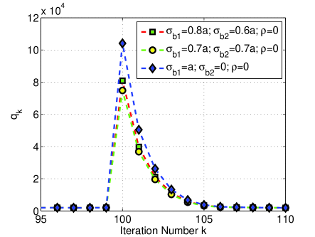
Refer to caption
Figure 2: The normalized MSE when independent biases are used. σb12+σb22=a2subscriptsuperscript𝜎2subscript𝑏1subscriptsuperscript𝜎2subscript𝑏2superscript𝑎2\sigma^{2}_{b_{1}}+\sigma^{2}_{b_{2}}=a^{2} for each case.
Figure 3: The normalized MSE for dependent biases. σb12+σb22=a2subscriptsuperscript𝜎2subscript𝑏1subscriptsuperscript𝜎2subscript𝑏2superscript𝑎2\sigma^{2}_{b_{1}}+\sigma^{2}_{b_{2}}=a^{2} for each case.

In Fig. 3, three dependent-noise attack strategies are compared, including the optimal one according to (39), allocating the power equally among the sensors, and allocating all the power to the sensor with smallest measurement error variance. It is clear that the optimal solution has the largest impact on the estimation performance, and it outperforms the best independent-noise attack strategy significantly.

VII-B Systems with Position and Velocity Sensors

We now consider the case where the adversary attacks Kalman filtering system with a vector sensor observation containing both position and velocity measurements. We first consider a single-sensor system, and the sensor has a position measurement variance of 3 and a velocity measurement variance of 4. We set the sum of σbp12superscriptsubscript𝜎subscript𝑏subscript𝑝12\sigma_{b_{p_{1}}}^{2} and T2σbv12superscript𝑇2superscriptsubscript𝜎subscript𝑏subscript𝑣12T^{2}\sigma_{b_{v_{1}}}^{2} to be 3000. In this particular case, w11w12+w21w22>0subscript𝑤11subscript𝑤12subscript𝑤21subscript𝑤220w_{11}w_{12}+w_{21}w_{22}>0, so the optimal choice is ρbp,bv=1subscript𝜌subscript𝑏𝑝subscript𝑏𝑣1\rho_{b_{p},b_{v}}=1. Based on Theorem 2, the best strategy is to set σbp=52.3subscript𝜎subscript𝑏𝑝52.3\sigma_{b_{p}}=52.3 and σbv=16.2subscript𝜎subscript𝑏𝑣16.2\sigma_{b_{v}}=16.2. It is clear from Fig. 4 that the strategy provided in Theorem 2 maximizes the MSE of Kalman filter system by injecting vector bias information.
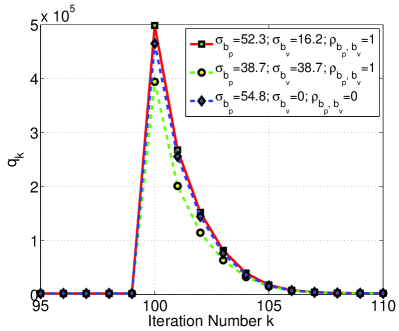
Refer to caption
Figure 4: The normalized MSE for a system with a single sensors. σp12+T2σv12=a2subscriptsuperscript𝜎2subscript𝑝1superscript𝑇2subscriptsuperscript𝜎2subscript𝑣1superscript𝑎2\sigma^{2}_{p_{1}}+T^{2}\sigma^{2}_{v_{1}}=a^{2} for each case.

Next we consider a system with two sensors. The first sensor is the same as the one described above, and the second one is with position measurement variance 4 and velocity measurement variance 5. In this particular case, again we have w11w12+w21w22>0subscript𝑤11subscript𝑤12subscript𝑤21subscript𝑤220w_{11}w_{12}+w_{21}w_{22}>0, so all the ρ𝜌\rhos in s1subscript𝑠1s_{1}, s2subscript𝑠2s_{2}, and s3subscript𝑠3s_{3} should be set as 1. We first use a systematic grid search to find an approximate globally optimal solution and then we use the FMINCON function in Matlab, a local search algorithm, to refine this approximate globally optimal solution. The optimal solution we have obtained is σbp12=1826,σbp22=1023,σbv12=81,σbv22=68formulae-sequencesuperscriptsubscript𝜎subscript𝑏subscript𝑝121826formulae-sequencesuperscriptsubscript𝜎subscript𝑏subscript𝑝221023formulae-sequencesuperscriptsubscript𝜎subscript𝑏subscript𝑣1281superscriptsubscript𝜎subscript𝑏subscript𝑣2268\sigma_{b_{p_{1}}}^{2}=1826,\sigma_{b_{p_{2}}}^{2}=1023,\sigma_{b_{v_{1}}}^{2}=81,\sigma_{b_{v_{2}}}^{2}=68. For comparison purpose, we also implement an attack strategy that allocate power equally among the observation components and among the two sensors, which is σbp12=σbp22=σbv12=σbv22=750superscriptsubscript𝜎subscript𝑏subscript𝑝12superscriptsubscript𝜎subscript𝑏subscript𝑝22superscriptsubscript𝜎subscript𝑏subscript𝑣12superscriptsubscript𝜎subscript𝑏subscript𝑣22750\sigma_{b_{p_{1}}}^{2}=\sigma_{b_{p_{2}}}^{2}=\sigma_{b_{v_{1}}}^{2}=\sigma_{b_{v_{2}}}^{2}=750. The simulation result is shown in Fig. 5. As we can see, the optimal attack strategy has a much greater impact than the one that allocates power equally. Based on the optimal solution, we can find that allocating more power to the measurement with lower variance will have a greater effect on Kalman filter system.
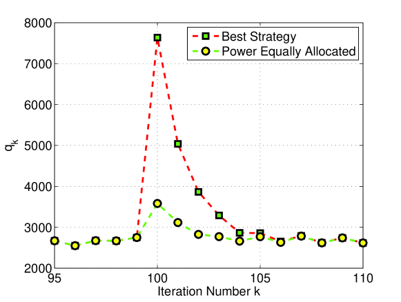
Refer to caption
Figure 5: The normalized MSE for a system with two sensors. σp12+σp22+T2σv12+T2σv22=a2superscriptsubscript𝜎subscript𝑝12superscriptsubscript𝜎subscript𝑝22superscript𝑇2superscriptsubscript𝜎subscript𝑣12superscript𝑇2superscriptsubscript𝜎subscript𝑣22superscript𝑎2\sigma_{p_{1}}^{2}+\sigma_{p_{2}}^{2}+T^{2}\sigma_{v_{1}}^{2}+T^{2}\sigma_{v_{2}}^{2}=a^{2} for each case.

VII-C Determinant case

Numerical results are presented in this section to illustrate the effectiveness of the proposed attack strategies. Assuming that the injected bias noise 𝐛ksubscript𝐛𝑘{\bf b}_{k} is zero-mean and Gaussian distributed, we can show that the posterior probability density function (PDF) of the target state conditioned on the past observations and the current corrupted observation is

p(𝐱K|𝐳1:K1,𝐳K)=𝒩(𝐱^K|K,𝐏K|K+𝐀K)𝑝conditionalsubscript𝐱𝐾subscript𝐳:1𝐾1subscriptsuperscript𝐳𝐾𝒩subscript^𝐱conditional𝐾𝐾subscript𝐏conditional𝐾𝐾subscript𝐀𝐾p({\bf x}_{K}|{\bf z}_{1:K-1},{\bf z}^{\prime}_{K})={\cal N}(\hat{\bf x}_{K|K},{\bf P}_{K|K}+{\bf A}_{K}) (102)

where 𝐱^K|Ksubscript^𝐱conditional𝐾𝐾\hat{\bf x}_{K|K} is the updated state estimate calculated by Kalman filter, which is unaware of the presence of the injected false information. Then the target state 𝐱Ksubscript𝐱𝐾{\bf x}_{K} will be in the following confidence region (or error ellipse)

{𝐱:(𝐱𝐱^K|K)T(𝐏K|K+𝐀K)1(𝐱𝐱^K|K)γ}conditional-set𝐱superscript𝐱subscript^𝐱conditional𝐾𝐾𝑇superscriptsubscript𝐏conditional𝐾𝐾subscript𝐀𝐾1𝐱subscript^𝐱conditional𝐾𝐾𝛾\displaystyle\left\{{\bf x}:({\bf x}-\hat{\bf x}_{K|K})^{T}({\bf P}_{K|K}+{\bf A}_{K})^{-1}({\bf x}-\hat{\bf x}_{K|K})\leq\gamma\right\} (103)

with probability determined by the threshold γ𝛾\gamma [23]. The volume of the confidence region defined by (103) corresponding to the threshold γ𝛾\gamma is

V(K)=cnx|γ(𝐏K|K+𝐀K)|1/2𝑉𝐾subscript𝑐subscript𝑛𝑥superscript𝛾subscript𝐏conditional𝐾𝐾subscript𝐀𝐾12V(K)=c_{n_{x}}|\gamma({\bf P}_{K|K}+{\bf A}_{K})|^{1/2} (104)

where nxsubscript𝑛𝑥n_{x} is the dimension of the target state 𝐱𝐱{\bf x},

cn=πn/2Γ(n/2+1)subscript𝑐𝑛superscript𝜋𝑛2Γ𝑛21\displaystyle c_{n}=\frac{\pi^{n/2}}{\Gamma(n/2+1)} (105)

and Γ()Γ\Gamma(\cdot) is the gamma function. First, let us consider a single-sensor case, where the sensor has a position measurement with noise variance of 333, which is independent of the velocity measurement with noise variance of 444. We set the bias noise power constraint as σbp2+T2σbv2=3000superscriptsubscript𝜎subscript𝑏𝑝2superscript𝑇2superscriptsubscript𝜎subscript𝑏𝑣23000\sigma_{b_{p}}^{2}+T^{2}\sigma_{b_{v}}^{2}=3000. We solve the optimization problem formulated in Section LABEL:sec:single-sensor numerically, and the optimal solution to (VI-B2) is σbp2=1500,σbv2=1500,ρbp,v=0.063formulae-sequencesubscriptsuperscript𝜎2subscript𝑏𝑝1500formulae-sequencesubscriptsuperscript𝜎2subscript𝑏𝑣1500subscript𝜌subscript𝑏𝑝𝑣0.063\sigma^{2}_{b_{p}}=1500,\sigma^{2}_{b_{v}}=1500,\rho_{b_{p,v}}=0.063. In Fig. 6, error ellipsis for different attack strategies are plotted. For all the different attack strategies, we set ρbp,v=0.063subscript𝜌subscript𝑏𝑝𝑣0.063\rho_{b_{p,v}}=0.063.

Refer to caption
Figure 6: Error ellipsis for different power allocation strategies

As we can see, under normal condition without false information injection, the error ellipse has the smallest area, while the optimal attack strategy leads to an error ellipse with the largest area. In Figs. 7 and 8, the volume (area) of the error ellipse is provided as a function of ρbp,vsubscript𝜌subscript𝑏𝑝𝑣\rho_{b_{p,v}} and the ratio κ=σbpσbvT𝜅subscript𝜎subscript𝑏𝑝subscript𝜎subscript𝑏𝑣𝑇\kappa=\frac{\sigma_{b_{p}}}{\sigma_{b_{v}}T}. We can see that when the κ=σbpσbvT=1𝜅subscript𝜎subscript𝑏𝑝subscript𝜎subscript𝑏𝑣𝑇1\kappa=\frac{\sigma_{b_{p}}}{\sigma_{b_{v}}T}=1, the area of the ellipse is maximized. Also from Figs. 7 and 8, it is clear that the area of ellipse increases as the absolute value of ρ𝜌\rho decreases. In Fig. 9, the trend of the error ellipsis as the ρ𝜌\rho changes from 11-1 to +11+1 is illustrated.

Refer to caption
Figure 7: Error ellipse volume
Refer to caption
Figure 8: Error ellipse volume
Refer to caption
Figure 9: Error ellipsis for different ρ𝜌\rhos

In this particular case, since σbp2+T2σbv2=3000superscriptsubscript𝜎subscript𝑏𝑝2superscript𝑇2superscriptsubscript𝜎subscript𝑏𝑣23000\sigma_{b_{p}}^{2}+T^{2}\sigma_{b_{v}}^{2}=3000, 𝚺Ksubscript𝚺𝐾\boldsymbol{\Sigma}_{K} is large and in (VI-B2) the second term (𝐖K𝚺K𝐖KTsubscript𝐖𝐾subscript𝚺𝐾subscriptsuperscript𝐖𝑇𝐾\mathbf{W}_{K}{\bf\Sigma}_{K}\mathbf{W}^{T}_{K}) dominates. Therefore, in (VI-B2) the identity matrix in the objective function is relatively small comparing to the second item, and approximately we have

|𝐈n+𝚺K𝐖KT𝐏K|K1𝐖K|subscript𝐈𝑛subscript𝚺𝐾subscriptsuperscript𝐖𝑇𝐾subscriptsuperscript𝐏1conditional𝐾𝐾subscript𝐖𝐾\displaystyle\left|{\bf I}_{n}+{\bf\Sigma}_{K}\mathbf{W}^{T}_{K}{\bf P}^{-1}_{K|K}\mathbf{W}_{K}\right|
|𝚺K||𝐖KT𝐏K|K1𝐖K|absentsubscript𝚺𝐾subscriptsuperscript𝐖𝑇𝐾subscriptsuperscript𝐏1conditional𝐾𝐾subscript𝐖𝐾\displaystyle\approx\left|{\bf\Sigma}_{K}\right|\left|\mathbf{W}^{T}_{K}{\bf P}^{-1}_{K|K}\mathbf{W}_{K}\right| (106)

The second term in the second line of the above equation is a constant. Hence, in order to get the maximum determinant, we should set σbp2=σbv2T2superscriptsubscript𝜎subscript𝑏𝑝2superscriptsubscript𝜎subscript𝑏𝑣2superscript𝑇2\sigma_{b_{p}}^{2}=\sigma_{b_{v}}^{2}T^{2} and ρbp,bv=0subscript𝜌subscript𝑏𝑝subscript𝑏𝑣0\rho_{b_{p},b_{v}}=0. This is almost the same solution as we have obtained numerically. Next we consider a system with two sensors. The first sensor is the same as the one described above, and the second one is with position measurement variance 444 and velocity measurement variance 555. To solve the optimization problem formulated in (100), we first use a systematic grid search to find an approximate globally optimal solution and then we use the FMINCON function in Matlab, a local search algorithm, to refine this approximate globally optimal solution. The optimal solution we have obtained is σbp12=1100,σbp22=600,σbv12=750,σbv22=550formulae-sequencesuperscriptsubscript𝜎subscript𝑏subscript𝑝121100formulae-sequencesuperscriptsubscript𝜎subscript𝑏subscript𝑝22600formulae-sequencesuperscriptsubscript𝜎subscript𝑏subscript𝑣12750superscriptsubscript𝜎subscript𝑏subscript𝑣22550\sigma_{b_{p_{1}}}^{2}=1100,\;\sigma_{b_{p_{2}}}^{2}=600,\;\sigma_{b_{v_{1}}}^{2}=750,\;\sigma_{b_{v_{2}}}^{2}=550,  ρbp1,p2=0.99,ρbp1,v1=0.83,ρbp1,v2=0.75,ρbv1,p2=0.89,ρbp2,v2=0.23,ρbv1,v2=0.95formulae-sequencesubscript𝜌subscript𝑏subscript𝑝1subscript𝑝20.99formulae-sequencesubscript𝜌subscript𝑏subscript𝑝1subscript𝑣10.83formulae-sequencesubscript𝜌subscript𝑏subscript𝑝1subscript𝑣20.75formulae-sequencesubscript𝜌subscript𝑏subscript𝑣1subscript𝑝20.89formulae-sequencesubscript𝜌subscript𝑏subscript𝑝2subscript𝑣20.23subscript𝜌subscript𝑏subscript𝑣1subscript𝑣20.95\rho_{b_{p_{1},p_{2}}}=0.99,\;\rho_{b_{p_{1},v_{1}}}=-0.83,\;\rho_{b_{p_{1},v_{2}}}=0.75,\;\rho_{b_{v_{1},p_{2}}}=0.89,\;\rho_{b_{p_{2},v_{2}}}=-0.23,\;\rho_{b_{v_{1},v_{2}}}=0.95. For comparison purpose, we introduce three sub-optimal attack strategies: Strategy I with all the ρ𝜌\rhos being 00s, and σbp12=1100,σbp22=600,σbv12=750,σbv22=550formulae-sequencesuperscriptsubscript𝜎subscript𝑏subscript𝑝121100formulae-sequencesuperscriptsubscript𝜎subscript𝑏subscript𝑝22600formulae-sequencesuperscriptsubscript𝜎subscript𝑏subscript𝑣12750superscriptsubscript𝜎subscript𝑏subscript𝑣22550\sigma_{b_{p_{1}}}^{2}=1100,\sigma_{b_{p_{2}}}^{2}=600,\sigma_{b_{v_{1}}}^{2}=750,\sigma_{b_{v_{2}}}^{2}=550; Strategy II with all the ρ𝜌\rhos being 111s, and σbp12=1100,σbp22=600,σbv12=750,σbv22=550formulae-sequencesuperscriptsubscript𝜎subscript𝑏subscript𝑝121100formulae-sequencesuperscriptsubscript𝜎subscript𝑏subscript𝑝22600formulae-sequencesuperscriptsubscript𝜎subscript𝑏subscript𝑣12750superscriptsubscript𝜎subscript𝑏subscript𝑣22550\sigma_{b_{p_{1}}}^{2}=1100,\sigma_{b_{p_{2}}}^{2}=600,\sigma_{b_{v_{1}}}^{2}=750,\sigma_{b_{v_{2}}}^{2}=550; and Strategy II with the ρ𝜌\rhos being the same as those for the optimal strategy, and σbp12=σbp22=σbv12=σbv22=750superscriptsubscript𝜎subscript𝑏subscript𝑝12superscriptsubscript𝜎subscript𝑏subscript𝑝22superscriptsubscript𝜎subscript𝑏subscript𝑣12superscriptsubscript𝜎subscript𝑏subscript𝑣22750\sigma_{b_{p_{1}}}^{2}=\sigma_{b_{p_{2}}}^{2}=\sigma_{b_{v_{1}}}^{2}=\sigma_{b_{v_{2}}}^{2}=750. The numerical results are shown in Fig. 10. As we can see, the optimal attack strategy has a greater impact than those sub-optimal attack strategies, resulting in the largest error ellipse.
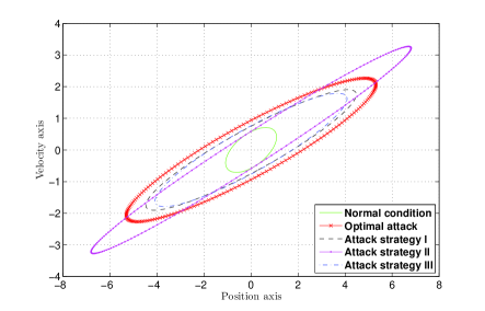
Refer to caption
Figure 10: Error ellipsis for different power allocation strategies

VIII Conclusions

In this paper, we derived the EMSE due to the injected random biases for a Kalman filter in a linear dynamic system. This allows us to find how to allocate the bias power among multiple sensors in order to maximize the effect of the false information on Kalman filter from two perspectives: trace and determinant. A concrete example of multi-sensor target tracking system has been provided. In this example, we investigated both the case where the sensors provide position measurements and the case where they collect both position and velocity measurements. Further, many closed-form results have been provided for the optimal attack strategies. In the future, we will use game theory and hypothesis testing techniques to characterize the model in order to have a better understanding of the false information attacks and Kalman filter defense against such attacks.

References

  • [1] J. Lu and R. Niu, “False Information Detection with Minimum Mean Squared Errors for Bayesian Estimation,” in Proc. The 49th Annual Conference on Information Systems and Sciences, Baltimore, Maryland, Mar 2015.
  • [2] Y. Liu, M.K. Reiter, and P. Ning, “False data injection attacks agianst state estimation in electric power grids,” in Proc. the 16th ACM Conference on Computer and Communications Security, Chicago, IL, November 2009.
  • [3] L. Jia, R.J. Thomas, and L. Tong, “Malicious data attack on real-time electricity market,” in Proc. International Conference on Acoustics, Speech, and Signal Processing, Prague, Czech Republic, May 2011, pp. 5952–5955.
  • [4] O. Kosut, L. Jia, R. J. Thomas, and L. Tong, “Malicious Data Attack on Smart Grid State Estimation: Attack Strategies and Countermeasures,” in Proc. First IEEE International Conference on Smart Grid Communications (SmartGridComm), Gaithersburg, MD, Oct. 2010, pp. 220–225.
  • [5] L. Jia, R. J. Thomas, and L. Tong, “On the nonlinearity effects on malicious data attack on power system,” in Power and Energy Society General Meeting, San Diego, CA, July 2012, pp. 1–8.
  • [6] M. A. Rahman and H. Mohsenian-Rad, “False data injection attacks with incomplete information against smart power grids,” in Proc. Global Communications Conference, San Diego, CA, Dec. 2012, pp. 3153–3158.
  • [7] J. Kim, L. Tong, and R. J. Thomas, “Data framing attack on state estimation,” IEEE Trans. on Aerospace and Electronic Systems, vol. 49, no. 3, pp. 1637–1653, July.
  • [8] X. Song, P. Willett, S. Zhou, and P. B. Luh, “The mimo radar and jammer games,” IEEE Trans. on Signal Processing, vol. 60, no. 2, pp. 687–699, February.
  • [9] J. Lu and R. Niu, “A State Estimation and Malicious Attack Game in Multi-Sensor Dynamic Systems,” in Proc. the 18th International Conference on Information Fusion, Washington, USA, Jul 2015.
  • [10] C. Yang, L. Kaplan, and E. Blasch, “Performance measures of covariance and information matrices in resource management for target state estimation,” IEEE Trans. on Aerospace and Electronic Systems, vol. 48, no. 3, pp. 2594–2612, July.
  • [11] C. Yang, L. Kaplan, E. Blasch, and M. Bakich, “Optimal placement of heterogeneous sensors for targets with gaussian priors,” IEEE Trans. on Aerospace and Electronic Systems, vol. 49, no. 3, pp. 1637–1653, July.
  • [12] M. P. Vitus and C J. Tomlin, “False data injection attacks against state estimation in electric power grids,” Sensor Placement for Improved Robotic Navigation.
  • [13] X. Lin and Y. Bar-Shalom, “Multisensor target tracking performance with bias compensation,” IEEE Trans. Aerosp. Electron. Syst., vol. 42, no. 3, pp. 1139–1149, July 2006.
  • [14] R. Niu and L. Huie, “System State Estimation in the Presence of False Information Injection,” in Statistical Signal Processing Workshop (SSP), Ann Arbor, MI, Aug. 2012, pp. 385–388.
  • [15] J. Lu and R. Niu, “False Information Injection Attack on Dynamic State Estimation in Multi-Sensor Systems,” in Proc. of the 17th International Conference on Information Fusion, Salamanca, Spain, July 2014.
  • [16] J. Lu and R. Niu, “Malicious Attacks on State Estimation in Multi-Sensor Dynamic Systems,” in Proc. IEEE Workshop on Information Forensics and Security, Atlanta, Georgia, USA, Dec 2014.
  • [17] J. Lu and R. Niu, “Sparse Attacking Strategies in Multi-Sensor Dynamic Systems Maximizing State Estimation Errors,” in Proc. 41st IEEE International Conference on Acoustics, Speech and Signal Processing, Shanghai, China, Mar 2016.
  • [18] J. Lu, R. Niu, and P. Han, “Optimal space-time attacks on system state estimation under a sparsity constraint,” in Proc. SPIE Sensors and Systems for Space Applications IX, April 2016.
  • [19] R. Niu, “Dynamic System State Estimation in the Presence of Continuous False Information Injection,” Tech. Rep., Extension Grant from Visiting Faculty Research Program, Air Force Research Laboratory Information Directorate, March 2012.
  • [20] Y. Bar-Shalom, X.R. Li, and T. Kirubarajan, Estimation with Applications to Tracking and Navigation, Wiley, New York, 2001.
  • [21] S. Boyd and L. Vandenberghe, Convex Optimization, Cambridge Univ. Press, Cambridge, U.K., 2004.
  • [22] B. Tang, J. Tang, and Y. Peng, “Mimo radar waveform design in colored noise based on information theory,” IEEE Trans. on Signal Processing, vol. 58, no. 9, pp. 4684 – 4697, September.
  • [23] Y. Bar-Shalom, P.K. Willett, and X. Tian, Tracking and Data Fusion: A Handbook of Algorithms, YBS Publishing, Storrs, CT, 2011.