Edge-Based Wedge Sampling to Estimate Triangle Counts in Very Large Graphs

Abstract

The number of triangles in a graph is useful to deduce a plethora of important features of the network that the graph is modeling. However, finding the exact value of this number is computationally expensive. Hence, a number of approximation algorithms based on random sampling of edges, or wedges (adjacent edge pairs) have been proposed for estimating this value. We argue that for large sparse graphs with power-law degree distribution, random edge sampling requires sampling large number of edges before providing enough information for accurate estimation, and existing wedge sampling methods lead to biased samplings, which in turn lead to less accurate estimations. In this paper, we propose a hybrid algorithm between edge and wedge sampling that addresses the deficiencies of both approaches. We start with uniform edge sampling and then extend each selected edge to form a wedge that is more informative for estimating the overall triangle count. The core estimate we make is the number of triangles each sampled edge in the first phase participates in. This approach provides accurate approximations with very small sampling ratios, outperforming the state-of-the-art up to 8 times in sample size while providing estimations with 95% confidence.

I Introduction

Graphs are heavily employed in modeling relationships, networks, and interactions of many real world applications. User interactions and usage patterns in social or mobile networks, compound/atom/amino-acid/molecule bonding/interaction tendencies in chemistry or biology, process/data/resource interaction/communication/dependency patterns in parallel/distributed systems can be listed among the examples where graph-based modeling is heavily used.

Triangles in a graph represent ternary relationships among the modeled objects/entities. The count of triangles in a graph is an important metric that can be used in determining the degree of clustering of the modeled networks. Graph metrics such as clustering coefficient [1] or transitivity ratio [2] make use of triangle count, and they are used as features for critical applications such as social network analysis [3], gene expression microarray data analysis [4], or text summarization [5].

Currently, the best known theoretical algorithm for identifying the exact number of triangles in a given graph ${\cal G}$ has a complexity of $O\left(m^{2\gamma/(\gamma+1)}\right)\approx O(m^{1.407})$ [6], where $m$ is the number of edges in ${\cal G}$, and $\gamma<2.372864$. This algorithm computes the third power of the adjacency matrix on the high-degree vertices and $\gamma$ is the exponent of the state-of-the-art matrix multiplication algorithm [7]. The practically used triangle counting and listing algorithms, however, take $O(m^{3/2})$ time [8]. Moreover, since finding the exact triangle count is computationally expensive for very large graphs with billions of edges that do not fit in memory, some studies focus on minimizing the number of disk I/Os performed [23, 24] during counting.

In many scenarios finding the exact triangle count is not necessary and an approximate number is sufficient as the graphs are very dynamic. A number of studies propose approximation solutions for estimating the triangle count [9, 10, 11, 12, 13, 14, 8, 15, 16]. These studies can be categorized based on the settings they consider: the streaming setting where graph components arrive as a data stream [9, 11, 10, 14], the semi-streaming setting where a constant number of passes over the edges are allowed [17, 18], and the static setting where the entire graph is available for analysis [13, 19, 15]. Another vein of studies consider efficient parallelization of this estimation process [20, 21, 22]. In this paper, we focus on the triangle count estimation problem under the static sequential setting. However, the intuition we provide can be used in a streaming setting as well.

The state-of-the-art approximation approaches are mostly based on random edge or wedge sampling. Random wedge sampling approaches first sample random vertices where vertex sampling probability is proportional to wedge participation probability of that vertex. After vertex sampling, two edges of each selected vertex are sampled to form wedges. The ratio of sampled wedges to closed wedges is used to estimate the number of triangles in the original graph [15]. When deployed on power-law degree graphs, wedge sampling approaches can suffer from bias (mostly high degree vertices are selected as hinge points of selected wedges), as they start with vertex sampling. Random edge sampling approaches count the number of triangles [13] or the number of wedges that are “closed” [16] (that have a third closing edge in the original graph) in the sampled subgraph, and use this count to estimate the triangle count. However, if graphs are sparse and the sampling ratio is low, these approaches can suffer from scarcity of valuable information (e.g. triangles, wedges) in the sampled subgraph.

We propose an algorithm for the graph triangle count estimation problem that combines the strong points of edge and wedge sampling while alleviating their deficiencies. Our approach starts with random edge sampling to avoid challenges arising in power-law graphs. Then we first estimate the number of triangles the sampled edges participate in the original graph. We use that first estimate to estimate the triangle count of the original graph. We accomplish this by turning the sampled edges into wedges in a second random edge selection phase and by checking if these sampled wedges are closed.

Our contributions can be listed as follows: (i) We propose an approach that offers highly accurate triangle count estimations even when employed over sparse power-law degree graphs and the sampling ratio is low. (ii) We theoretically prove the bounds of our algorithm and show with experiments that found bounds are tight. We also provide theoretical bounds for the state-of-the-art approaches. (iii) We theoretically and practically show that the proposed approach achieves up to eight times sampling size reduction over the state-of-the-art on large-scale real-world graphs.

The remainder of this paper is organized as follows. We present existing approximation approaches in Section II along with our observations that led to the development of the proposed algorithm. Section III discusses details of our proposed edge-based wedge selection algorithm. We provide a theoretical analysis of the proposed method and other methods in the literature in Section IV. We evaluate the performance of the proposed method and compare it against the state-of-the-art in Section V. In Section VI we conclude.

II Counting Triangles in a Graph

Given an undirected graph ${\cal G}=({\cal V},{\cal E})$ defined by a set of vertices ${\cal V}$ and a set ${\cal E}$ of pairwise relations (edges) among vertices in ${\cal V}$, we would like to estimate $\Delta$, the number of triangles (three edge cycles) in ${\cal G}$. Approximation approaches to this problem mostly consider randomly sampling edges or adjacent edge pairs (wedges) from the original graph ${\cal G}$ and try to estimate the number of triangles in ${\cal G}$ based on analysis conducted on the sampled graph entities.

Existing approximation methods have certain deficiencies when applied to graphs modeling real networks that exhibit power-law degree distributions with many low-degree vertices and few very high-degree vertices [25]. Using the current random edge sampling methods, sampled subgraphs can be too sparse to reveal sufficient information for accurate estimation when low sampling ratios are employed. Using the current random wedge-sampling methods, the uniformity on the wedge selection scheme favors high-degree vertices, and this leads to less accurate estimations.

In the remainder of this section, we explain the state-of-the-art edge and wedge sampling based approaches in detail, discuss their strengths and deficiencies, and provide our intuitions to address these deficiencies. In Table I we summarize the important notations that we use in our discussions and in the remainder of the paper.

II-A Random edge sampling

Random edge sampling based approaches first construct a subgraph ${{\cal G}}_{S}$ of ${\cal G}$ by traversing over each edge in ${\cal E}$ and adding each edge to the subgraph ${{\cal G}}_{S}$ with probability $p$. They then extract features from ${{\cal G}}_{S}$ for estimating $\Delta$.

II-A1 Counting triangles in ${{\cal G}}_{S}$

The idea of random edge sampling to construct a subgraph ${{\cal G}}_{S}$ was first proposed by Tsourakakis et al. [13]. In their work, they use the number of triangles in ${{\cal G}}_{S}$ to estimate $\Delta$ as ${\Delta}_{S}/p^{3}$, where ${\Delta}_{S}=\left|\{(u,v,w)~{}|~{}(u,v),(v,w),(w,u)\in{{\cal G}}_{S}\}\right|$. This estimation is based on the fact that all three edges of any triangle in ${{\cal G}}_{S}$ has to be selected with probability $p$ from ${\cal G}$. A drawback of this approach is that when $p$ is small, ${{\cal G}}_{S}$ is very unlikely to contain even one triangle, making this approach impractical for small sampling ratios.

II-A2 Counting closed wedges in ${{\cal G}}_{S}$

Recently, Etemadi et al. [16] proposed an approach that improves upon [13]. They first identify all of the wedges formed in ${{\cal G}}_{S}$, and then check for edges in ${\cal G}$ to determine whether the wedges in ${{\cal G}}_{S}$ are closed in ${\cal G}$. That is, for any wedge $u-$$v$$-w$ in ${{\cal G}}_{S}$, they check whether the third edge $(w,u)$ is in ${\cal G}$ or not. They use the count of such closed wedges to estimate $\Delta$ as ${\Lambda}_{S}^{+}/3p^{2}$, where ${\Lambda}_{S}^{+}$=$\left|\{(u,v,w)~{}|~{}(u,v),(v,w)\in{{\cal G}}_{S},(w,u)\in{\cal G}\}\right|$. This estimation is due to the following two facts that the two edges forming a wedge in ${{\cal G}}_{S}$ have to be independently selected with probability $p$, and that any triangle contains three wedges.

Symbol	Description
${\cal G}$	Original graph with vertex set ${\cal V}$ and edge set ${\cal E}$
$\Delta$	Number of triangles in ${\cal G}$
$\Lambda$	Number of wedges in ${\cal G}$
${{\cal G}}_{S}$	Random subgraph by edge selection
${\Delta}_{S}$	Number of triangles in ${{\cal G}}_{S}$
${\Lambda}_{S}^{+}$	Number of closed wedges in ${{\cal G}}_{S}$
$T(e)$	Number of triangles in ${\cal G}$ that contain edge $e$
${T}_{S}$	Sum of $T(e)$ for edges in ${{\cal G}}_{S}$: $\sum_{e\in{{\cal G}}_{S}}T(e)$
$\tau$	Estimate on ${T}_{S}$ (EWSample)
$d_{u}$	Degree of vertex $u$
$\delta(e)$	Degree of lower degree end vertex of edge $e$=$(u,v)$:
	$\delta(e)$=$min(d_{u},d_{v})$
$\sigma(t)$	Sum of $\delta(e)$ for edges in triangle $t$: $\sum_{e\in t}\delta(e)$

TABLE I: Summary of the notations.

Although [16] enables selection of smaller $p$ values compared to the proposed approach in [13], we note that achieving accurate estimates still requires a large sampling probability $p$ as the chance of observing sufficient number of wedges remains low when sampling edges from large sparse graphs. In particular, for a graph ${\cal G}$ with $m$ edges and $\Delta$ triangles, the expected number of wedges in the sampled graph that is part of a triangle in the original graph is $3\Delta p^{2}$ [16] . In our subsequent experiments, $\Delta$ can be in the order of $10^{10}$, and we would like to support $p$ values in the range $[10^{-5},10^{-6}]$. In such a scenario, clearly, the number of closed wedges in the sampled subgraph (each of which form a triangle in the original graph) will be too low to provide accurate estimations.

II-A3 Strengths of edge-based sampling approaches

Random edge-based sampling methods do not require any previous knowledge on the structure of ${\cal G}$ and can be applied without any preprocessing. Furthermore, in power-low graphs, factoring computations over edges instead of vertices can alleviate challenges associated with the power-law degree distribution of vertices and can also ease parallelism [26].

II-A4 Deficiencies of edge-based sampling approaches

The core problem of existing edge-based sparsification approaches is that the relationship between the findings they extract from the sampled graph ${{\cal G}}_{S}$ and the estimation they make for triangle count in ${\cal G}$ is a cubic or quadratic function of $p$. This prevents accurate estimation for low $p$ values. Ideally, the estimation should be directly proportional to $p$.

II-A5 Proposed improvement over edge sampling

The intuition behind our proposed approach is similar in nature to the improvement proposed by [16] over [13]. In [16], they point out that instead of counting entities that appear with probability $p^{3}$ (triangles in ${{\cal G}}_{S}$), they can count entities that appear with probability $p^{2}$ (closed wedges in ${{\cal G}}_{S}$) and thus enable using lower sampling ratios while achieving the same accuracy. In this work, we take one more step further and estimate $\Delta$ using entities that appear with probability $p$.

In our approach, we also start with randomly selecting a set of edges ${{\cal E}}_{S}\subset{\cal E}$. Then, using each edge $e$ in ${{\cal E}}_{S}$, we directly estimate the number of triangles that $e$ is a part of. More formally, let $T(e)$ be the number of triangles in ${\cal G}$ that $e$ is a part of. Furthermore, let ${T}_{S}$ be the total number of triangles in ${\cal G}$ that each edge in ${{\cal E}}_{S}$ is a part of, i.e. ${T}_{S}=\sum_{e\in{{\cal E}}_{S}}T(e)$. In our approach, we estimate ${T}_{S}$, which can also be written as: ${T}_{S}=\left|\{(u,v,w)~{}|~{}(u,v)\in{{\cal E}}_{S},(v,w),(w,u)\in{\cal G}\}\right|$. We call our estimation for ${T}_{S}$ as $\tau$ and further estimate $\Delta$ as $\tau/3p$, since an edge can be selected with probability $p$ and since each triangle has three edges. Our estimate of ${T}_{S}$ is directly proportional to $p$. We explain in detail how we estimate ${T}_{S}$ and why the probability associated with ${T}_{S}$ estimation is proportional to $p$ in Section III and Section IV respectively.

II-B Random wedge sampling

Random wedge sampling approaches extract wedges from ${\cal G}$ and analyze properties of extracted wedges to estimate $\Delta$.

II-B1 Uniform wedge sampling

Random uniform wedge sampling for triangle counting was first proposed by Schank and Wagner [27]. More recently, Seshadhri et al. [19, 15] analyze this approach in depth for counting various triadic measures, including counting triangles. Similar appraoches have also been considered in a streaming setting [14].

In a nutshell, uniform random wedge sampling first picks a vertex $v$ in ${\cal V}$ based on the number of wedges hinging at $v$ and then investigates if a randomly created wedge that consists of two randomly selected edges of $v$ is a closed wedge or not. The ratio of closed wedges to sampled wedges is used to estimate $\Delta$ by multiplying one third of the ratio with $\Lambda$, the total number of wedges in ${\cal G}$. This estimation is based on the fact that there are three different closed wedges for each triangle in ${\cal G}$.

II-B2 Strengths of uniform wedge sampling

This approach does not get adversely impacted from the sparsity of graphs and can support small sampling probabilities as each sampled entity (wedge) is an entity of interest and overall search target (the number of triangles in the graph) is directly proportional to the findings about sampled entities (ratio of closed wedges).

II-B3 Deficiencies of uniform wedge sampling

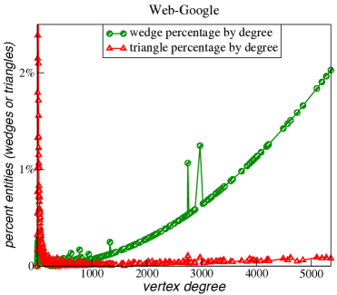
For graphs with power-law degree distributions, triangles are not uniformly distributed across wedges, as shown on an example in Figure 1. In this figure, we present the percentage of wedges hinging at vertices with a given degree (indicated via green circles) and the percentage of triangles that vertices with a given degree participate in (indicated via red triangles) for a real-world power-law Web graph from Google [28]. As can be seen from the figure, the uniform wedge sampling approach would select more wedges hinging at higher degree vertices simply because there are more such wedges. In fact, as expected, as the vertex degree $d$ increases, the number of wedges hinging at vertices with degree $d$ increases almost quadratically. However, the number of triangles that vertices with degree $d$ participate in have a linear relationship with the degree. These characteristics demonstrate that uniform wedge sampling will provide biased estimations. We observe similar characteristics in many real world networks and they become more prominent as graphs grow larger and sparser.

Figure 1: Wedge and triangle distribution per vertex degree for the Web-Google dataset [28].

It is also important to note that, for applying uniform wedge sampling, one needs to compute the degree distribution of the vertices and the number of wedges in ${\cal G}$; therefore, such approaches require a preprocessing step which takes linear time in the number of edges.

II-B4 Proposed improvement over uniform wedge sampling

To avoid favoring high degree vertices, our algorithm starts by random edge sampling instead of uniform wedge sampling. We then extend each sampled edge to a wedge, and check for the existence of the closing edge in ${\cal G}$ to determine whether the vertices of the wedge define a triangle or not. To increase the accuracy of our estimate, we only consider the wedges that hinge at the lower degree vertex of the selected edges. By selecting random edges in the first step, we ensure that we start with a good sampling distribution. Note that the probability of sampling a wedge in our schema is linearly proportional with the degree of the vertex that the wedge hinges at, whereas for uniform wedge sampling, that probability is quadratically proportional with the degree of the hinge vertex.

III Edge-Based Wedge Sampling

(a) Example graph ${\cal G}$ with 11 vertices, 16 edges, and 5 triangles. Sampling probability $p$ is given as $p$=$3/16$.

(b) Random edge sampling over the example graph ${\cal G}$ provides three selected edges: ${{\cal E}}_{S}$=${\{(v_{2},v_{5}),(v_{1},v_{4}),(v_{7},v_{8})\}}$.

(c) Informed wedge sampling for selected edges. Each wedge hinges on the lower degree end of the initially selected edges.

(d) Triangle check in ${\cal G}$. Wedges hinging at $v_{4}$, $v_{8}$ form triangles, $\tau$$=$$(d_{v_{4}}-1)$$+$$(d_{v_{8}}-1)$$=$$3$. Estimate is $\tau/3p\approx 5.33$.

Figure 2: Illustration of EWSample on an example graph.

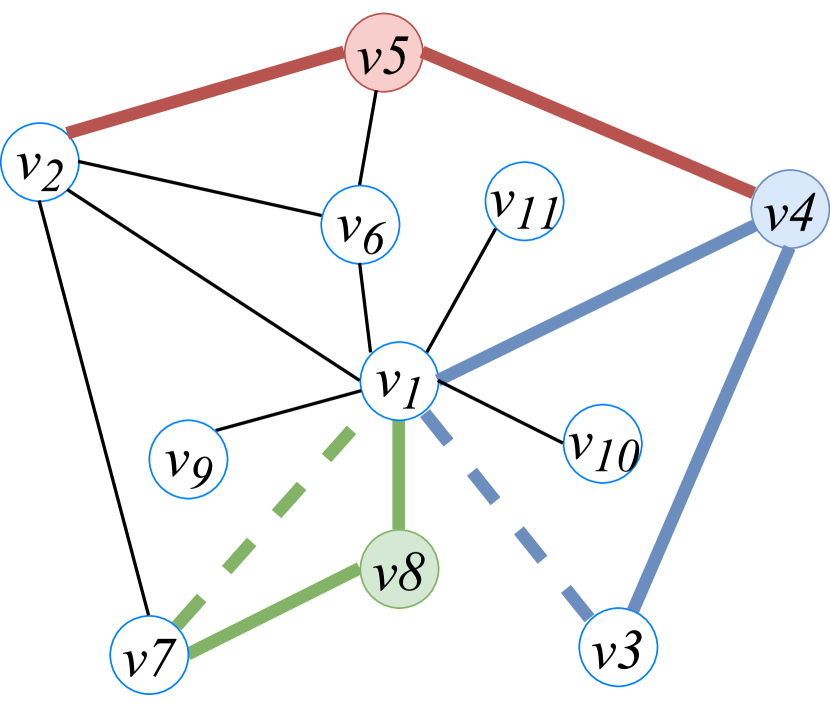
Our approach to estimating the number of triangles in ${\cal G}$ is based on sampling a set of edges ${{\cal E}}_{S}$ and estimating the number of triangles in ${\cal G}$ that the sampled edges are part of. To accomplish this, after sampling a set of edges ${{\cal E}}_{S}$ in a first step, we keep sampling further edges in a second step to form wedges with each sampled edge in ${{\cal E}}_{S}$. To increase the accuracy of our estimate, in the second step, we only consider edges that form wedges hinging at the lower degree vertices of the edges selected in the first step. In a third step, we perform a check for the third edge to determine whether the vertices of a selected wedge define a triangle or not. If any such wedge is closed, we estimate the number of triangles the originally sampled edge contributes in to be the degree of its lower-end vertex. If a sampled wedge is not closed, we estimate the number of triangles the originally sampled edge contributes in to be zero. Using these estimates, we then estimate the total number of triangles in the original graph.

Since our approach is initially based on random edge sampling, we do not need to perform a preprocessing step to obtain degree distributions of vertices in ${\cal G}$; we only consider degrees of vertices of sampled edges ${{\cal E}}_{S}$. Furthermore, via edge sampling, we avoid being highly biased towards high degree vertices. By constructing wedges via a second sampling stage we ensure that all sampled edges turn into entities of interest. By selecting low-end of each sampled edge as wedge hinge points, we reduce the search space. Finally, by making an estimation associated with each sampled edge (i.e. the number of triangles that edge participates in), we ensure that our overall estimation correlates linearly with the sampling size, which enables us to significantly reduce sampling ratio.

Next, we discuss in detail our edge-based wedge selection and triangle estimation algorithm EWSample. Pseudocode of EWSample is depicted in Algorithm 1. Given a graph ${\cal G}$ and a sampling probability $p$, we first randomly sample edges ${{\cal E}}_{S}$ as shown in lines 2–5. For any edge $e=(u,v)\in{{\cal E}}_{S}$ selected in the first step, let us assume $d_{v}\leq d_{u}$ without loss of generality. In lines 6–7, for any selected edge in ${{\cal E}}_{S}$, we randomly select one more edge, say $(v,w)$ among the remaining edges incident to $v$ to form a path or wedge $u$-$v$-$w$. In lines 8–9, we check for the existence of the edge $(u,w)$ in the original graph. If the original graph indeed contains the edge $(u,w)$, we increment the total triangle count $\tau$ by $d_{v}-1$. That is, if the sampled wedge originating from $e=(u,v)$ is closed and forms a triangle, then we estimate $T(e)$, the number of triangles $e$ participates in, as the number of edges adjacent to $e$ at $v$, which is equal to $d_{v}-1$. The rationale of this estimation is based on a single wedge, hence, we estimate $T(e)$ to be 0 or $d_{v}-1$ depending on the outcome. Finally, in line 10, we return $\tau/3p$ as an estimate for $\Delta$ since a triangle can be counted by all of its three edges’ estimates. The complexity of our algorithm is $O(m)$: the subgraph sampling takes $O(m)$ time, and the rest of the algorithm takes $O(pm)$ time.

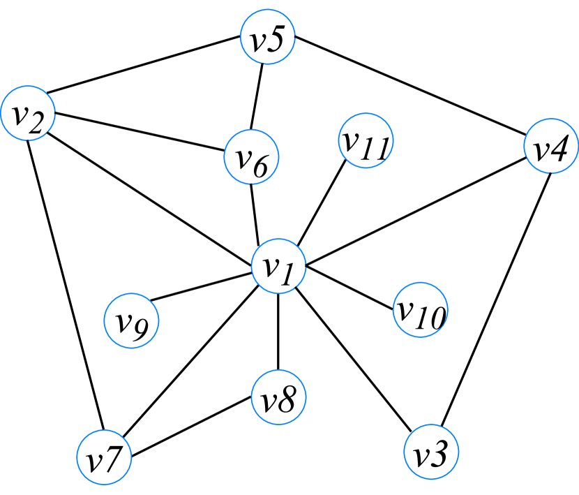
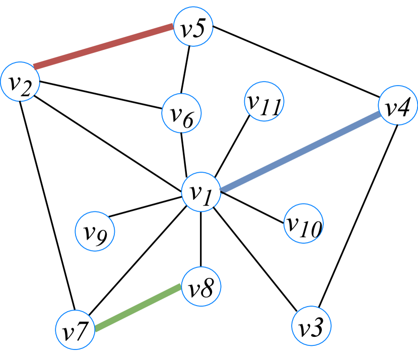
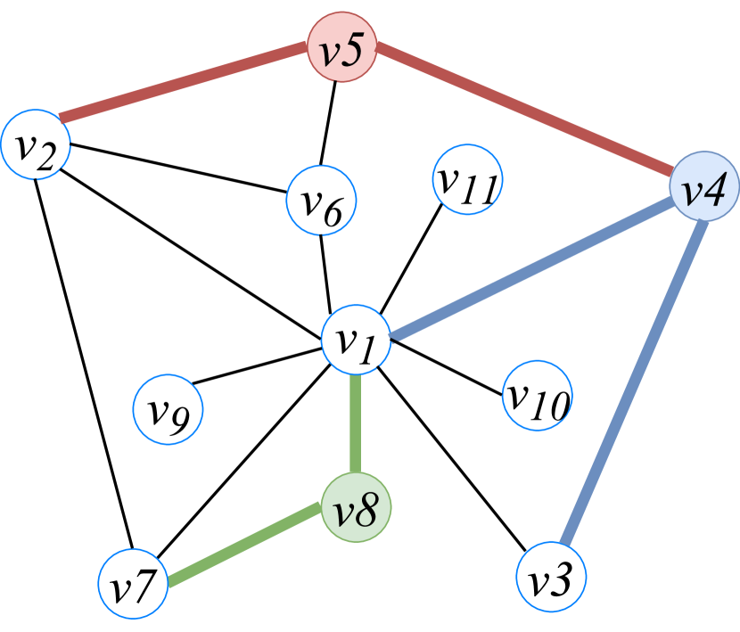
We illustrate our algorithm EWSample on an example (see Figure 2). Our example graph ${\cal G}$ contains 11 vertices, 16 edges and 5 triangles (Figure 2(a)). The triangles are $\{v_{1},v_{2},v_{6}\},\{v_{1},v_{2},v_{7}\},\{v_{1},v_{3},v_{4}\},\{v_{1},v_{7},v_{8}\},$ and $\{v_{2},v_{5},v_{6}\}$. Running EWSample with probability $p=3/16$, let us assume that the sampled edges ${{\cal E}}_{S}$ in the first step are $(v_{2},v_{5}),(v_{1},v_{4}),$ and $(v_{7},v_{8})$ (Figure 2(b)). In the second step, we randomly select an edge incident to the low degree vertices of these edges (Figure 2(c)); for $e=(v_{2},v_{5})$ let the randomly selected edge be $e^{\prime}=(v_{5},v_{4})$, for $e=(v_{1},v_{4})$ let $e^{\prime}=(v_{4},v_{3})$, and for $e=(v_{7},v_{8})$ let $e^{\prime}=(v_{8},v_{1})$ (note that the last selection is with probability 1 since $d_{v_{8}}-1=1$). Then, we compute $\tau$ based on whether these wedges are closed or not (Figure 2(d)): $v_{2}$$-$$v_{5}$$-$$v_{4}$ is not closed so that wedge does not increase $\tau$, but the other two wedges $v_{1}$$-$$v_{4}$$-$$v_{3}$ and $v_{7}$$-$$v_{8}$$-$$v_{1}$ are closed and they both increase $\tau$ by their low degrees - 1 respectively. In particular, $\tau$ gets increased by 2 for the edge $(v_{1},v_{4})$ and by 1 for the edge $(v_{7},v_{8})$. Finally, EWSample outputs the final estimate as:

$$\frac{\tau}{3p}=\frac{3}{3\times\frac{3}{16}}=\frac{16}{3}\approx 5.33$$

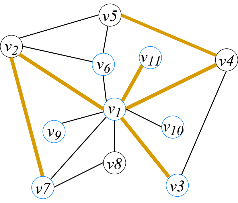
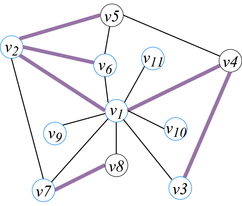
To compare our approach to existing approaches, Figure 3(a) showcases a potential run of the algorithm proposed in [15] with a sampling rate of $p=3/16$, i.e., $k=3$ random wedges. As seen in the figure, their randomly selected wedges are $v_{1}$$-$$v_{4}$$-$$v_{5}$, $v_{1}$$-$$v_{2}$$-$$v_{7}$, and $v_{11}$$-$$v_{1}$$-$$v_{3}$, and only one of them is closed: $v_{1}$$-$$v_{2}$$-$$v_{7}$. In this graph number of wedges $\Lambda=56$, therefore their estimate can be calculated as:

$$1\times\frac{\Lambda}{3k}=\frac{56}{9}\approx 6.22$$

Figure 3(b) showcases a potential run of the algorithm proposed in [16]. One can argue that since our approach and uniform wedge sampling work with wedges, the random edge sampling method should be allowed to pick twice the number of edges. However, note that random edge selection requires constructing the subgraph ${{\cal G}}_{S}$, and identifying all the wedges in ${{\cal G}}_{S}$, which can be very costly. Practically, sampling an edge and sampling a wedge have similar costs and algorithms should be compared based on their performance when they sample the same number of entities (edges or wedges).

We note that when $p$ is very low, finding even one closed wedge using the algorithm in [16] becomes very difficult even in our simple example. So we pick twice the number of edges to be able to find some closed wedges in the sampled graph, i.e., we use a sampling rate of $2p$. As seen in the figure, their sample graph contains 6 edges and these sampled edges form 4 wedges. Out of these 4 wedges, ${\Lambda}_{S}^{+}=3$ of them are closed: $v_{5}$$-$$v_{2}$$-$$v_{6}$, $v_{1}$$-$$v_{2}$$-$$v_{6}$, and $v_{1}$$-$$v_{4}$$-$$v_{3}$. Noting that the probability used in their first step is $3/8$, their estimate can be computed as:

$$\frac{{\Lambda}_{S}^{+}}{3p^{2}}=\frac{3}{3\times(\frac{3}{8})^{2}}=\frac{64}{9}\approx 7.11$$

Algorithm 1 EWSample(${\cal G}=({\cal V},{\cal E}),p$)

1:  $\tau\leftarrow 0$, $\ {{\cal E}}_{S}\leftarrow\emptyset$

2:  for each edge $e\in{\cal E}$ do

3:     randomly select edge $e=(u,v)$ with probability $p$

4:     if $e$ is selected then

5:        ${{\cal E}}_{S}\leftarrow{{\cal E}}_{S}\cup{\{e\}}$

6:  for each selected edge $e=(u,v)\in{{\cal E}}_{S}$ do

7:     randomly select an edge $e^{\prime}=(v,w)$ incident to $v$, where $d_{v}\leq d_{u}$ and $w\neq u$

8:     if $e^{\prime\prime}=(u,w)\in{\cal E}$ then

9:        $\tau\leftarrow\tau+d_{v}-1$

10:  return $\tau/3p$

(a) Random-wedge sampling algorithm proposed in [15]. Out of the 3 sampled wedges, only 1 wedge is closed. Estimate is $56/9$$\approx$$6.22$.

(b) Random-edge sampling and wedge counting algorithm proposed in [16]. The edges form 4 wedges, 3 of which are closed. Estimate is $64/9$$\approx$$7.11$.

Figure 3: Illustration of applying the state-of-the-art approaches: (a) uniform wedge sampling approach proposed in [15], and (b) random edge sampling approach proposed in [16].

IV Expected Value, Variance, and RSE

We analyze the expected value, variance, and relative standard error (RSE) of our estimate $\tau$ in order to investigate the confidence interval of the outputs of EWSample. We also analyze the same terms for the state-of-the-art approaches to provide theoretical comparisons. We provide the theoretical analysis in this section, and show empirical evidences that corroborate our theory in the next section.

IV-A Expected Value, Variance, and RSE of EWSample

To provide this analysis we first express our output in terms of indicator variables. First, we number the edges in the original graph as $e_{1},\ldots,e_{m}$. For any given edge $e_{i}$, we represent each of the $T(e_{i})$ triangles that $e_{i}$ participates in by the wedges that hinge on the lower degree vertex of $e_{i}$. To that extent, we number each such edge that belongs to a triangle with $e_{i}$ and adjacent to $e_{i}$ on the lower degree vertex. Letting these edges be $e_{i1},\ldots,e_{iT(e_{i})}$, we define our indicator variable $w_{ij}$ as the indicator for selecting $e_{i}$ in the first step and $e_{ij}$ in the second step as the wedge for $e_{i}$. Finally, defining $\delta(e_{i})$ to be the degree of the lower degree vertex of $e_{i}$, we express $\tau$, our estimate for ${T}_{S}$ as:

$$\tau=\sum_{i=1}^{m}\sum_{j=1}^{T(e_{i})}w_{ij}\cdot(\delta(e_{i})-1).$$

Using this expression, we show that the expected value of $\tau$ is $3p\Delta$, and thus the expected value of the output of EWSample is $\Delta$.

Lemma 1.

The expected value of $\tau$ is $3p\Delta$.

Proof.

We have $\tau=\sum_{i=1}^{m}\sum_{j=1}^{T(e_{i})}w_{ij}\cdot(\delta(e_{i})-1)$ for the EWSample algorithm. Hence:

$$\mathbb{E}(\tau)=\sum_{i=1}^{m}\sum_{j=1}^{T(e_{i})}\mathbb{E}(w_{ij})\cdot(\delta(e_{i})-1)$$

The probability that $w_{ij}=1$ is $p/(\delta(e_{i})-1)$, therefore:

$$\mathbb{E}(\tau)=\sum_{i=1}^{m}\sum_{j=1}^{T(e_{i})}p=\sum_{i=1}^{m}pT(e_{i})=3p\Delta$$

where the latter equality holds as each triangle is counted in each of its edges’ $T(e)$ values. ∎

Next, we argue that the variance of $\tau$ is low, however, our arguments involve some features of the original graph ${\cal G}$. More specifically, the variance of $\tau$ involves the terms $K$ and $\phi$, where $K$ is the number of pairs of triangles that share an edge in ${\cal G}$ [16], and we define $\phi$ as $\phi=\sum_{i=1}^{\Delta}\sigma(t_{i})-3$, where $\sigma(t_{i})$ is the sum of $\delta(e)$ for edges in triangle $t_{i}$: $\sigma(t_{i})=\sum_{e\in t_{i}}\delta(e)$. Intuitively, one can think of $\phi$ as the sum of the degrees of each vertex in each triangle in ${\cal G}$, except that instead of summing the maximum degree vertex, the sum involves the minimum degree vertex twice. This is due to fact that we select the low degree vertex of the initially selected edge as hinge point in our edge-based wedge construction mechanism.

Lemma 2.

The variance of $\tau$ is $p\phi-p^{2}(3\Delta+2K)$, where $\phi=\sum_{i=1}^{\Delta}\sigma(t_{i})-3$.

Proof.

Since the indicator variables $w_{i_{1}j_{1}}$ and $w_{i_{2}j_{2}}$ are independent for $i_{1}\neq i_{2}$, we have:

$$var(\tau)=\sum_{i=1}^{m}var\left(\sum_{j=1}^{T(e_{i})}w_{ij}\cdot(\delta(e_{i})-1)\right)$$

This can be rewritten as

$$var(\tau) =\sum_{i=1}^{m}\left(\sum_{j=1}^{T(e_{i})}(\delta(e_{i})-1)^{2}\cdot var(w_{ij})\right.$$

$$+\left.\sum_{j\neq k}(\delta(e_{i})-1)^{2}\cdot covar(w_{ij},w_{ik})\right)$$

We have $var(w_{ij})=(p/(\delta(e_{i})-1)-p^{2}/(\delta(e_{i})-1)^{2})$ and since we are selecting only one wedge for each edge, we have $covar(w_{ij},w_{ik})=(0-p^{2}/(\delta(e_{i})-1)^{2})$. Further simplifying:

$$var(\tau) =\sum_{i=1}^{m}\left(\sum_{j=1}^{T(e_{i})}p\cdot(\delta(e_{i})-1)-\sum_{j=1}^{T(e_{i})}p^{2}-\sum_{j\neq k}p^{2}\right)$$

$$=p\sum_{i=1}^{m}T(e_{i})\cdot(\delta(e_{i})-1)-p^{2}\sum_{i=1}^{m}T(e_{i})$$

$$-p^{2}\sum_{i=1}^{m}T(e_{i})(T(e_{i})-1)$$

The first term can be written as a sum over the triangles where for each triangle, the value $\delta(e)-1$ is summed for each of its edges. The second term can be written in terms of $\Delta$, the number of triangles in ${\cal G}$. And, the third term can be written in terms of $K$, the number of pairs of triangles that share an edge in ${\cal G}$. Finally, we prove:

$$var(\tau)=p\left(\sum_{i=1}^{\Delta}\sigma(t_{i})-3\right)-p^{2}(3\Delta+2K)$$

where $\sigma(t_{i})$ is the sum of $\delta(e)$ for edges in triangle $t_{i}$. ∎

In order to compare our method to previous work, we use the Relative Standard Error (RSE) values of all of the methods and base our arguments on the RSE values. Applying the formula for the relative standard error $RSE(\tau)=\sqrt{var(\tau)}/\mathbb{E}(\tau)$, we obtain:

$$RSE(\tau) =\frac{\sqrt{p\phi-p^{2}(3\Delta+2K)}}{3p\Delta}=\sqrt{\frac{\phi}{9p\Delta^{2}}-\frac{3\Delta+2K}{9\Delta^{2}}}$$

The above formula is complex, however, we can approximate it by simply dropping the negative term inside the square root. We argue that this will not affect our actual RSE values too much since the $p$ values we choose for our experiments will be very low, and in addition the actual value of the negative term, $(3\Delta+2K)/9\Delta^{2}$, will be too low for the graphs we consider making the negative term very insignificant. Therefore, we approximate our RSE using the following formula:

$$RSE(\tau)\approx\sqrt{\frac{\phi}{9p\Delta^{2}}}$$ (1)

where $\phi=\sum_{i=1}^{\Delta}\sigma(t_{i})-3$ is a constant depending only on the original graph ${\cal G}$. In our experiments, we show that we achieve RSE values that are very close to the approximation we provide in Equation 1.

IV-B RSE of Other Methods

We also analyze the expected value, variance, and the RSE of the other methods to offer a theoretical comparison with our method. We consider two state-of-the-art methods, the method introduced by Etemadi et al. [16], which we call EdgeSample, as well as the method introduced by Seshadhri at al. [15], which we call WedgeSample.

We begin with the analysis of WedgeSample, the method introduced by Seshadhri et al. [15]. We define indicator variables for each of the $3\Delta$ closed wedges in order to express the random variable that counts the number of closed wedges observed in WedgeSample. Letting $w_{i}$ to be an indicator for the $i^{th}$ closed wedge, indicator for whether it is one of the randomly selected $k=pm$ wedges, we define:

$$\omega=\sum_{i=1}^{3\Delta}w_{i}$$

Using $\omega$, WedgeSample outputs $\omega\Lambda/3k$ to estimate $\Delta$. In the next lemma, we provide the expected value and the variance analysis of $\omega$ to be used in the relative standard error analysis of $\omega$, where $C=3\Delta/\Lambda$ is the clustering coefficient:

Lemma 3.

The expected value of $\omega$ is $pmC$, and the variance of $\omega$ is $pmC(1-C)\left(1-\frac{pm-1}{\Lambda-1}\right)$.

Proof.

We have $\mathbb{E}(\omega)=\sum_{i=1}^{3\Delta}\mathbb{E}(w_{i})=\sum_{i=1}^{3\Delta}k/\Lambda=3\Delta k/\Lambda$, which implies $\mathbb{E}(\omega)=pmC$ by definition.

For variance, we have $var(w_{i})=\frac{k}{\Lambda}(1-\frac{k}{\Lambda})$. Also, we have $covar(w_{j},w_{k})=\frac{k}{\Lambda}(\frac{k-1}{\Lambda-1}-\frac{k}{\Lambda})$ for any $w_{j}\neq w_{k}$. Therefore, we write variance as:

$$var(\omega) =\sum_{i=1}^{3\Delta}var(r_{i})+\sum_{j\neq k}covar(r_{j},r_{k})$$

$$=3\Delta\frac{k}{\Lambda}\left(1-\frac{k}{\Lambda}\right)+3\Delta(3\Delta-1)\frac{k}{\Lambda}\left(\frac{k-1}{\Lambda-1}-\frac{k}{\Lambda}\right)$$

$$=kC\left(1-\frac{k}{\Lambda}\right)+kC(3\Delta-1)\left(\frac{k-1}{\Lambda-1}-\frac{k}{\Lambda}\right)$$

$$=kC\left(1-\frac{k-1}{\Lambda-1}+3\Delta\left(\frac{k-1}{\Lambda-1}-\frac{k-1}{\Lambda}-\frac{1}{\Lambda}\right)\right)$$

$$=kC\left(1-\frac{k-1}{\Lambda-1}+3\Delta\frac{k-1}{\Lambda(\Lambda-1)}-3\Delta\frac{1}{\Lambda}\right)$$

The last equation simplifies as $pmC(1-C)\left(1-\frac{pm-1}{\Lambda-1}\right)$ proving the variance stated in the lemma. ∎

Using this lemma, we obtain the formula for their relative standard error $RSE(\omega)=\sqrt{var(\omega)}/\mathbb{E}(\omega)$:

$$RSE(\omega) =\frac{\sqrt{pmC(1-C)\left(1-\frac{pm-1}{\Lambda-1}\right)}}{pmC}$$

$$=\sqrt{\frac{1-C}{pmC}\left(1-\frac{pm-1}{\Lambda-1}\right)}$$

Similarly, we can drop the insignificant negative terms from the above formula and get an approximation with fewer simpler terms:

$$RSE(\omega)\approx\sqrt{\frac{1-C}{pmC}}$$ (2)

TABLE II: Datasets used in experiments and their features.

Dataset	$n$	$m$	$\Delta$	$C$$=$$\frac{3\Delta}{\Lambda}$	$\frac{3\Delta}{m}$	$\frac{\phi}{3\Delta}$	$\frac{K}{\Delta}$	Description
Ego-Facebook [29]	4K	88K	1612K	0.5192	54.8	115.5	141.9	Online social network (OSN) in Facebook
Enron-email [28]	36K	183K	727K	0.0853	11.9	102.1	50.2	Email communication network in Enron
Brightkite [29]	58K	214K	494K	0.1106	6.9	76.6	59.1	OSN in Brightkite
Dblp-coauthor [29]	317K	1049K	2224K	0.3064	6.4	37.6	47.2	Co-authorship network in DBLP
Amazon [29]	334K	925K	667K	0.2052	2.2	7.1	5.3	Co-purchasing network from Amazon
Web-NotreDame [28]	325K	1090K	8910K	0.0877	24.5	119.4	174.2	Web graph of Notre Dame
Citeseer [28]	384K	1736K	1351K	0.0496	2.3	26.6	11.6	Citation network in Citeseer
Dogster [28]	426K	8543K	83499K	0.0143	29.3	1085.2	503.8	OSN from dogster.com website
Web-Google [28]	875K	4322K	13391K	0.0552	9.3	35.4	46.4	Web graph from Google
YouTube [29]	1134K	2987K	3056K	0.0062	3.1	257.7	82.4	OSN in Youtube
DBLP [28]	1314K	5362K	12184K	0.1703	6.8	38.0	35.8	Co-authorship network in DBLP
As-skitter [29]	1696K	11095K	28769K	0.0054	7.8	796.4	713.3	Internet connections from Skitter project
Flicker [28]	2302K	22838K	837605K	0.1076	110.0	1239.9	732.8	Online social network in Flicker
Orkut [28]	3072K	117185K	627584K	0.0413	16.1	371.3	106.9	Online social network in Orkut
LiveJournal [29]	3997K	34681K	177820K	0.1253	15.4	204.3	222.1	OSN in LiveJournal
Orkut2 [30]	11514K	327036K	223127K	0.0003	2.0	1229.0	155.4	OSN in Orkut
Web-Arabic [30]	22743K	553903K	36895360K	0.0313	199.8	2047.7	3042.7	Web graph from Arabian countries
MicrosoftAG [31]	46742K	528463K	578188K	0.0151	3.3	97.1	33.9	Citation network from Microsoft Academic
Twitter [28]	41652K	1202513K	34824916K	0.0008	86.9	11638.5	5061.5	OSN from Twitter
Friendster [28]	65608K	1806067K	4173724K	0.0174	6.9	311.6	44.4	OSN of website Friendster

In the next section, we provide empirical evidence that verifies the above approximation given in Equation 2.

Next, we analyze EdgeSample, the method proposed by Etemadi et al. [16]. Once again, we define an indicator variable for each of the $3\Delta$ closed wedges in order to express the closed wedge count of this method. Letting $r_{i}$ to be an indicator for the $i^{th}$ closed wedge, indicator for whether it is included in ${{\cal G}}_{S}$ in the first step of EdgeSample, we define:

$$\rho=\sum_{i=1}^{3\Delta}r_{i}$$

Using $\rho$, EdgeSample outputs $\rho/3p^{2}$ to estimate $\Delta$. In the next lemma, we provide the expected value and variance of $\rho$ based on the discussion from their original work [16]:

Lemma 4.

The expected value of $\rho$ is $3p^{2}\Delta$, and the variance of $\rho$ is $3\Delta(p^{2}-p^{4})+8K(p^{3}-p^{4})$.

Using this lemma, we obtain the formula for their relative standard error $RSE(\rho)=\sqrt{var(\rho)}/\mathbb{E}(\rho)$:

$$RSE(\rho) =\frac{\sqrt{3\Delta(p^{2}-p^{4})+8K(p^{3}-p^{4})}}{3p^{2}\Delta}$$

$$=\sqrt{\frac{1}{3p^{2}\Delta}-\frac{1}{3\Delta}+\frac{8K}{9p\Delta^{2}}-\frac{8K}{9\Delta^{2}}}$$

Once again, we can drop the insignificant negative terms from the above formula to get an approximation with fewer simpler terms.

$$RSE(\rho)\approx\sqrt{\frac{1}{3p^{2}\Delta}+\frac{8K}{9p\Delta^{2}}}$$ (3)

Note that the approximation in Equation 3 is different than the one in proposed in the work of Etemadi et al. [16] and the main reason to include the extra term is to ensure a much better approximation. In the next section, we verify the validity of our approximation schemes and argue that we can simply use the theoretical approximations to compare the performance of the three methods.

V Evaluation

In this section, we provide an empirical and theoretical evaluation of the proposed algorithm.

V-A Experimental Setup

We compare the performance of our edge-based wedge sampling algorithm (EWS) with the state-of-the-art edge sampling (ES) and wedge sampling (WS) approaches proposed by Etemadi et al. [16] and Seshadhri et al. [15] both theoretically and experimentally using graphs modeling real-world large-scale networks. We also corroborate the theoretical analysis we provided in Section IV with empirical evidence. In the forthcoming experiments and analysis, we sample the same number of entities for the three different approaches; edges for ES, and wedges for WS and EWS. All approaches perform closed wedge checks as necessary; however, we do not account for the cost of those checks. In practice, the costs are almost exactly the same for WS and EWS, however, ES performs more checks as it considers closed wedge checks for any pair of adjacent edges in the sampled subgraph.

For comparison and also in order to verify our theoretical analysis, we observe the relative standard error ($RSE$) values of different algorithms for each of the datasets and compare these values with the theoretical analysis we provided in Section IV.

In order to provide comparable results, as was done in [16], we either fix the sampling probability, and report the corresponding RSE values of the three algorithms, or fix an RSE value and report the corresponding sampling rates. We calculate the experimental $RSE$ values observed with $k$ different runs of the algorithms using the formula:

$$RSE=\frac{\sqrt{\frac{1}{k}\sum_{i=1}^{k}(\Delta_{i}-\mu)}}{\Delta},$$

where $\Delta_{i}$ is the estimate obtained in the $i$-th run and $\mu$ is the mean of all of the $k$ runs, i.e., $\mu=\frac{1}{k}\sum_{i=1}^{k}\Delta_{i}$. In all of our experiments, we use $k=1000$.

The experiments are conducted on a server with 16 CPUs and 64 GB of RAM. In our experimental analysis we use 20 real-world datasets that were also used in [16]. These datasets vary in size; largest containing vertices in the order of ten millions and triangles in the order of ten billions, and the smallest containing vertices in the order of thousands and triangles in the order of millions. Features of these datasets are presented in Table II.

In addition to graph features, we also provide metrics of graphs that impact the performance of ES, WS and EWS in Table II as well. For example the higher the value of global clustering coefficient $C=3\Delta/\Lambda$, the better the performance of WS, as the chances of finding closed wedges during sampling increase. Similarly, $3\Delta/m$ indicates the number of triangles an average edge participates in a graph, and the higher this number the better the performance of EWS in general. EWS performance also gets impacted from the value of $\phi/3\Delta$ as well, which can be considered as the degree of the lowest degree or medium degree vertex in an average triangle. The higher this number gets, the courser the estimations made by EWS, hence the worse its performance. A similar argument can be made for ES and $K/\Delta$.

V-B Empirical Analysis and Verification of Theory

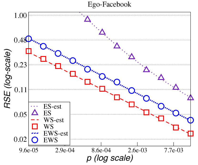
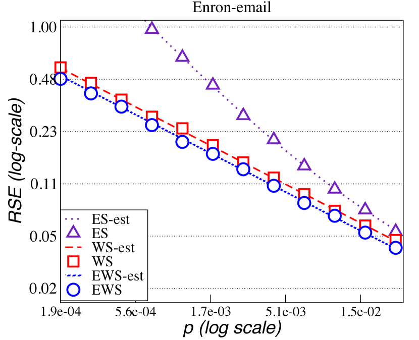
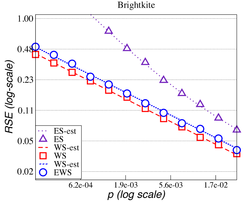
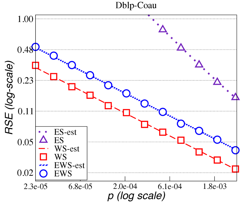
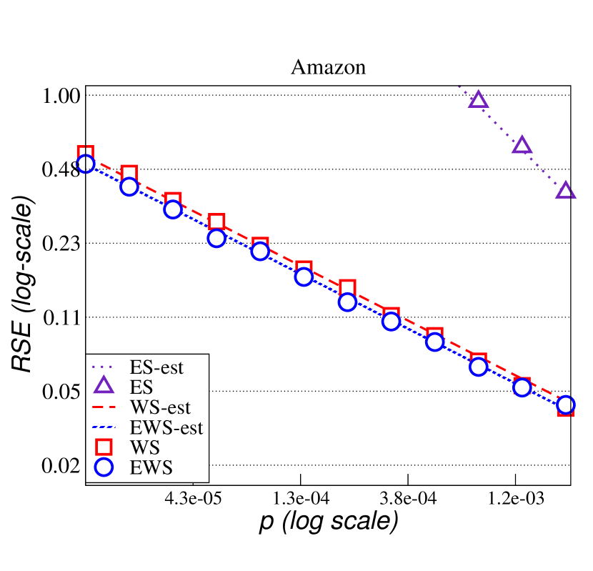
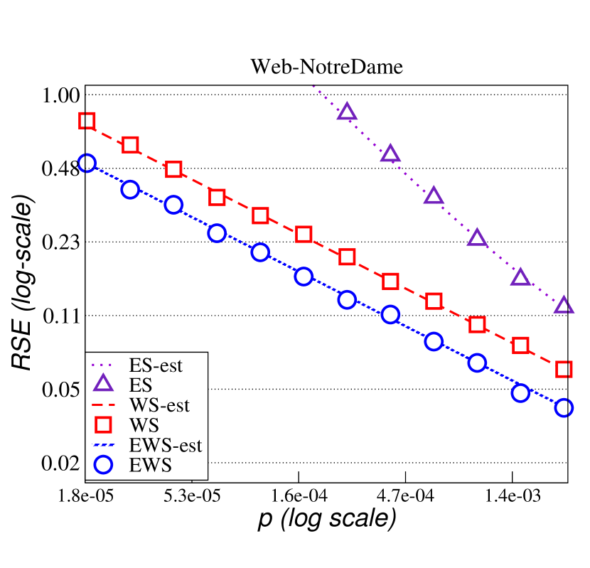
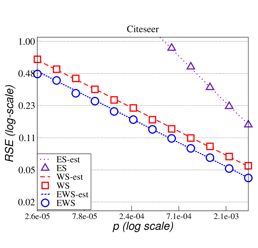
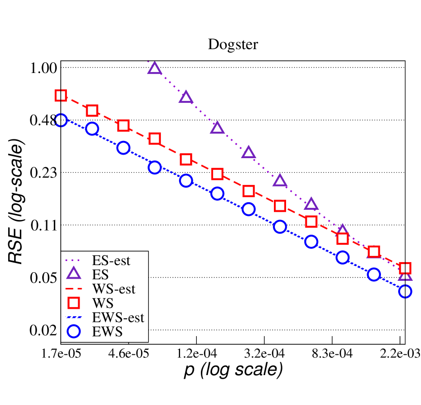
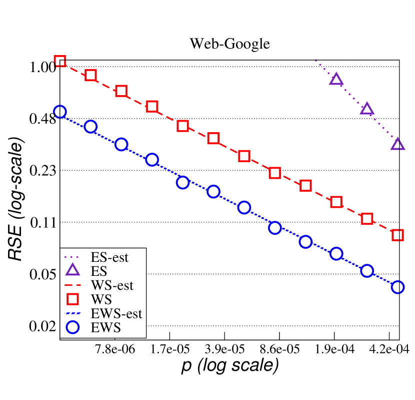
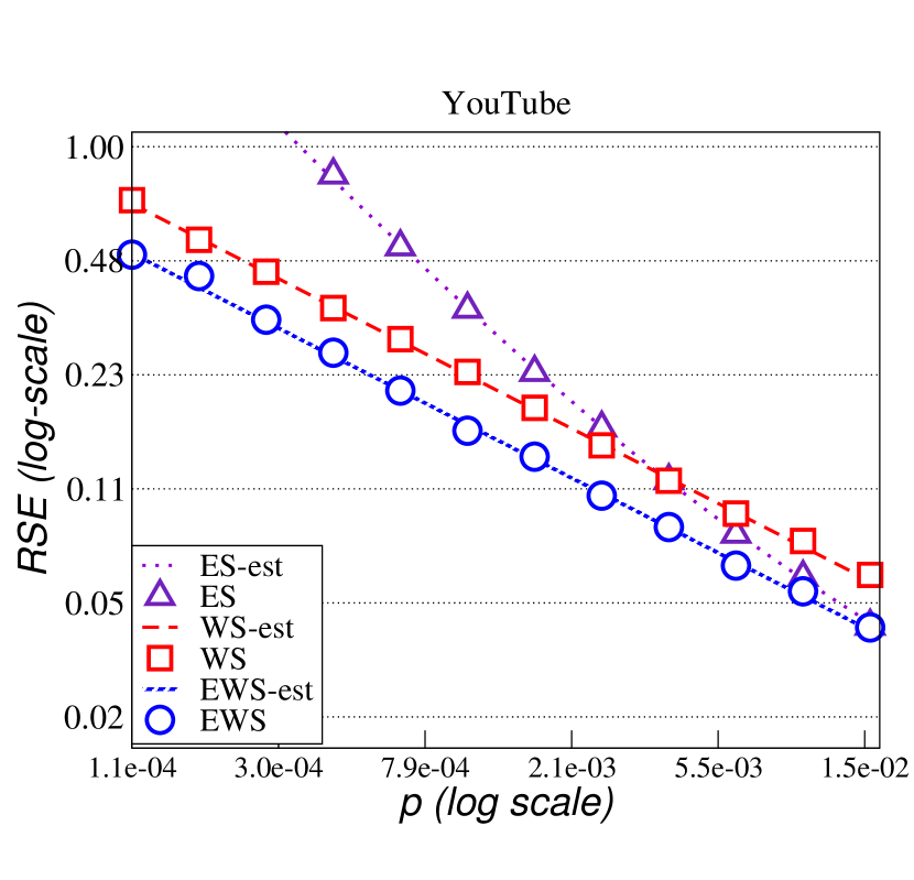
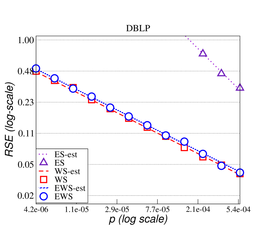
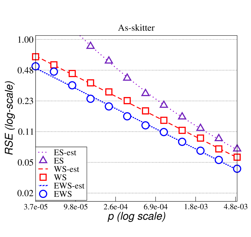
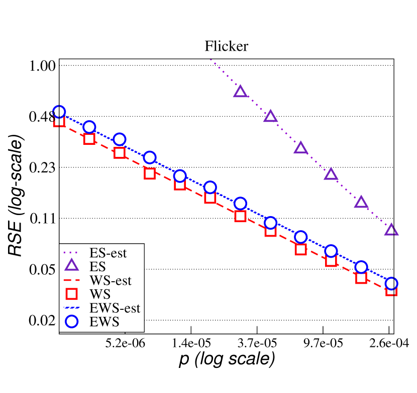
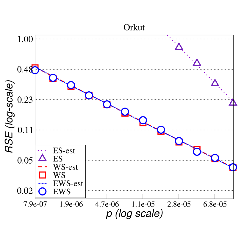
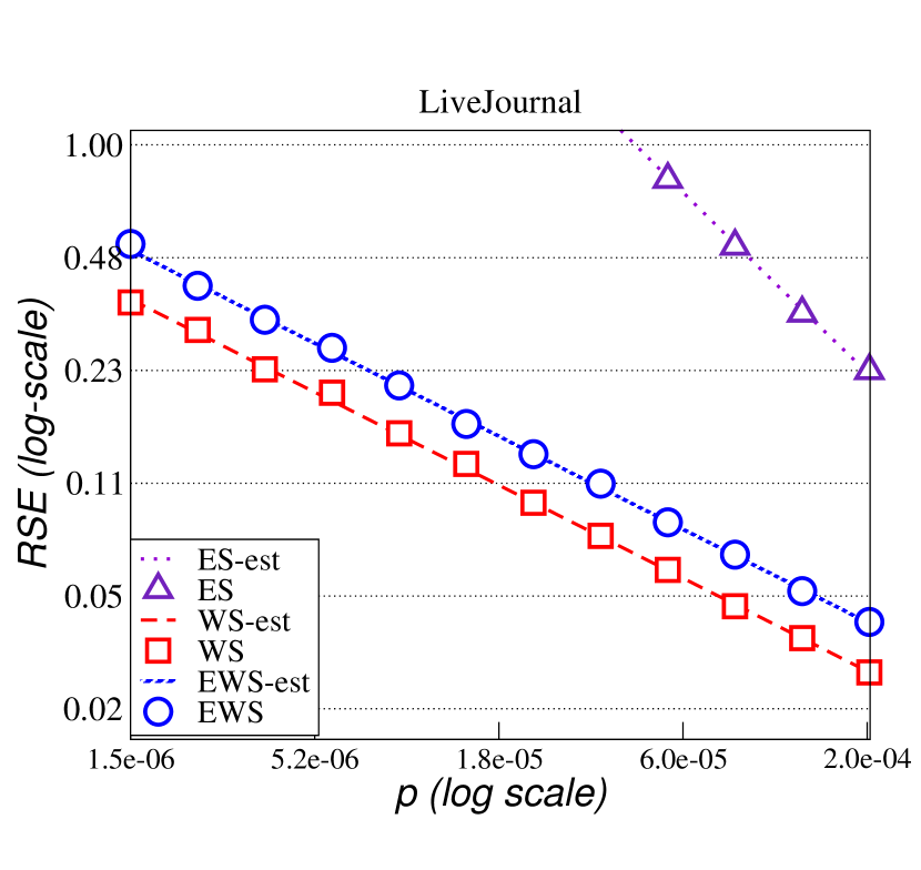
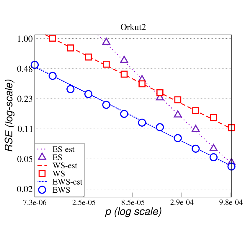
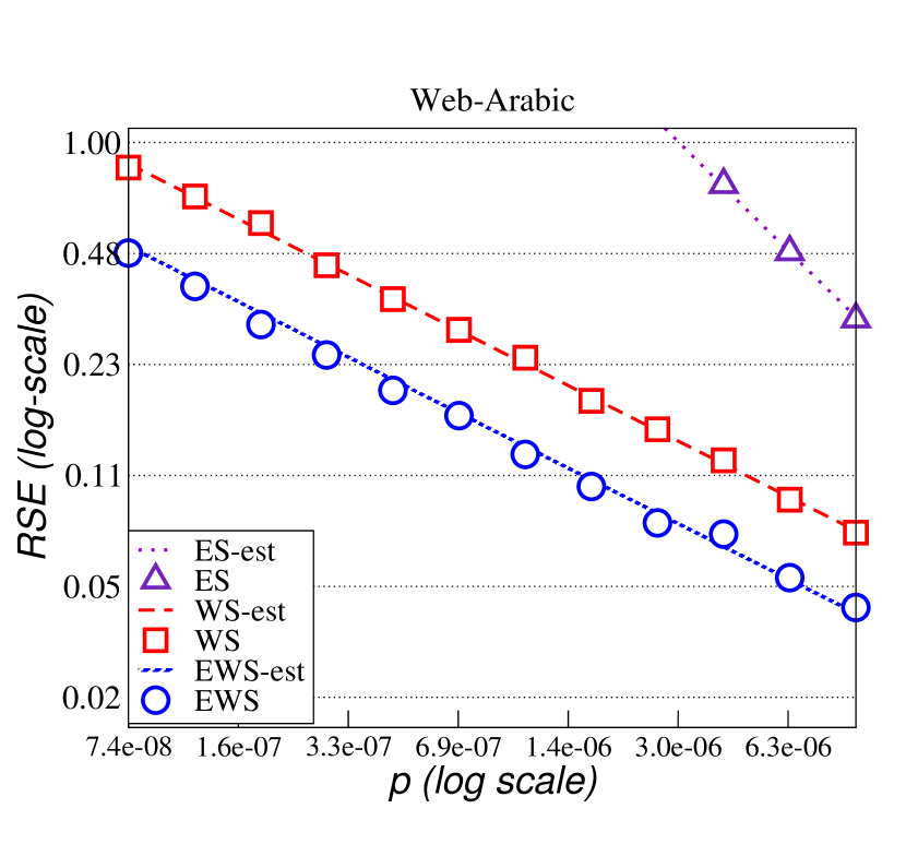
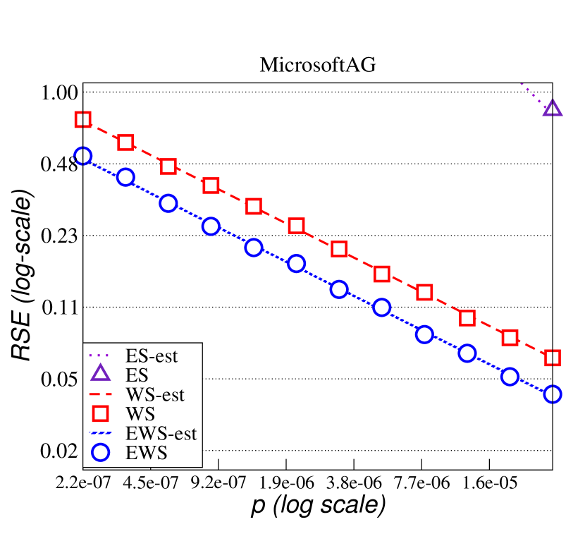
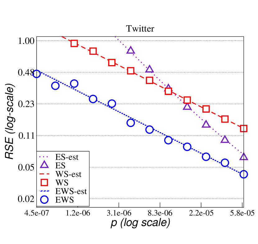
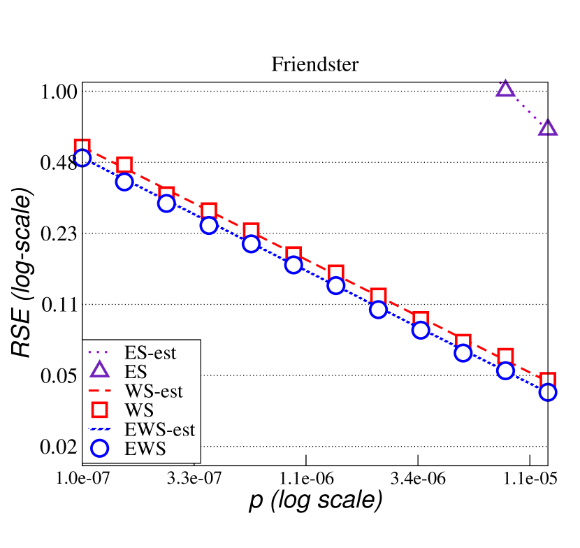
Figure 4, provides an empirical analysis of ES, WS, and EWS over the 20 datasets listed in Table II. The figure also depicts the RSE estimations indicated by Equations 1, 2, and 3 for EWS, WS, and ES, respectively. In this figure, the $x$-axis ranges between the sampling probabilities that provides $RSE$ values between 0.50 and 0.04 for EWS and we report the corresponding RSE values for ES, WS, and EWS when using the same sampling rates.

For all datasets depicted in Figure 4, the empirical RSE observations we make for EWS, WS, and ES match the theoretical bounds EWS-est, WS-est, and ES-est that we compute using Equations 1, 2, and 3, respectively. This proves the validity of our theoretical analysis.

Interestingly, we can observe in Figure 4 that the datapoints for EWS and WS follow a similar pattern and they exhibit parallel trends irrespective of the sampling ratio. In fact, this is to be expected as the theoretical $RSE$ approximations in Equations 1 and 2 both depend linearly on the sampling ratio and hence the estimations EWS-est and WS-est are parallel. Therefore, the ratio of their RSE values remain the same accross various sampling probabilities. Whichever of these two algorithms will perform better is based on the parameters of the graph. In 14 of the datasets EWS performs better than WS and in 6 datasets WS performs better than EWS. We note that since this is a log-log figure, the slight difference between the two lines in fact indicate a multiplicative difference.

In Figure 4, for all datasets and most $p$ values, EWS and WS perform significantly better than ES. On the other hand, the slope for ES-est is much steeper—also to be expected because of the quadratic dependence on the sampling ratio—and even though ES provides much higher RSE values for low $p$ values, as $p$ increases, the accuracy of ES increases significantly.

(a) Ego-Facebook.

(b) Enron-email.

(c) Brightkite.

(d) Dblp-Coau.

(e) Amazon.

(f) Web-NotreDame.

(g) Citeseer.

(h) Dogster.

(i) Web-Google.

(j) YouTube.

(k) DBLP.

(l) As-skitter.

(m) Flicker.

(n) Orkut.

(o) LiveJournal.

(p) Orkut2.

(q) Web-Arabic.

(r) MicrosoftAG.

(s) Twitter.

(t) Friendster.

Figure 4: $RSE$ vs $p$ for the 20 datasets.

TABLE III: Sample sizes to achieve RSE=0.05.

Dataset	$m$	$ES$	$WS$	$EWS$	$\frac{WS}{EWS}$
Ego-Facebook	88K	2978	370	843	0.44
Enron-email	183K	5619	4288	3443	1.25
Brightkite	214K	10299	3217	4417	0.73
Dblp-coauthor	1049K	13005	905	2369	0.38
Amazon	925K	14460	1549	1316	1.18
Web-NotreDame	1090K	9459	4162	1948	2.14
Citeseer	1736K	20102	7660	4554	1.68
Dogster	8543K	23326	27631	14805	1.87
Web-Google	4322K	16556	6842	1525	4.49
Youtube	2987K	38692	63923	33586	1.90
DBLP	5362K	20763	1949	2228	0.87
As-skitter	11095K	103336	73852	40950	1.80
Flicker	22838K	13332	3315	4507	0.74
Orkut	117185K	57679	9293	9244	1.01
LiveJournal	34681K	38703	2791	5314	0.52
Orkut2	327036K	296516	1519667	240184	6.33
Web-Arabic	553903K	42394	12363	4098	3.02
MicrosoftAG	528463K	259340	26135	11836	2.21
Twitter	1202513K	111704	472194	53584	8.81
Friendster	1806067K	326237	22621	17976	1.26

To provide a deeper understanding of the difference between the three algorithms we compare, we also present Table III, where we fix the RSE to 0.05 (95% confidence value) and compare the number of sampled entities that allows all approaches to achieve this given RSE value using the theoretic approximations from Equations 1, 2, and 3. As seen in the table, in all datasets either EWS or WS provides the lowest sampling size. Hence, in the last column of the table we provide the ratio of the sampling sizes for WS and EWS. Similar to the results provided in Figure 4, in 14 datasets the $\frac{WS}{EWS}$ value is higher than one, indicating that EWS outperforms WS, and for 6 datasets it is lower. Furthermore, because the RSE values of both approaches depend linearly on the sampling ratio, the $\frac{WS}{EWS}$ ratio in Table III would remain the same if some other fixed RSE value was used instead.

Noticeably, the datasets that WS outperforms EWS are datasets with high global clustering coefficient values (e.g. $C\geq 0.1$). This is expected as in these datasets the probability of observing closed wedges when sampling wedges increase significantly and the advantage of EWS over WS is lost. However, EWS outperforms WS for all graphs with low global clustering coefficient values ($C<0.1$) as the performance of WS is directly tied to this coefficient. We also note that advantage of EWS over WS becomes more prominent as the sizes of graphs increase.

Complexity of EWS, ES, and WS are all $O(m)$ and practical runtimes of these algorithms with low sampling ratios over very large graphs are very fast. As an example, on the Twitter dataset, with a sampling ratio of $p\approx 0.00006$, EWS, ES, and WS takes 1.12, 1.11, and 0.26 seconds.

VI Conclusion

We proposed an edge-based wedge sampling approach for estimating the number of triangles in very large power-law degree graphs. Our approach combines the benefits of edge and wedge sampling to offer highly accurate estimations even for very large sparse graphs and for very low sampling ratios. Furthermore, it does not require any preprocessing to be performed over the graphs. Through analysis conducted over graphs modeling large-scale real-world networks, we theoretically and empirically show that our approach offers highly confident estimations and up to eight times sampling size reduction over the state-of-the-art alternatives even when the sampling ratio is low.

References

- [1] M. E. Newman, “The structure and function of complex networks,” SIAM review, vol. 45, no. 2, pp. 167–256, 2003.
- [2] S. Wasserman and K. Faust, Social network analysis: Methods and applications. Cambridge university press, 1994, vol. 8.
- [3] Z. Yang, C. Wilson, X. Wang, T. Gao, B. Y. Zhao, and Y. Dai, “Uncovering social network sybils in the wild,” ACM Transactions on Knowledge Discovery from Data (TKDD), vol. 8, no. 1, p. 2, 2014.
- [4] G. Kalna and D. J. Higham, “A clustering coefficient for weighted networks, with application to gene expression data,” AI Commun., vol. 20, no. 4, pp. 263–271, Dec. 2007.
- [5] Y. A. AL-Khassawneh, N. Salim, and O. A. Isiaka, “Extractive text summarisation using graph triangle counting approach: Proposed method,” in 1 st International Conference of Recent Trends in Information and Communication Technologies in Universiti Teknologi Malaysia, Johor, Malaysia, 2014, pp. 300–311.
- [6] N. Alon, R. Yuster, and U. Zwick, “Finding and counting given length cycles,” Algorithmica, vol. 17, no. 3, pp. 209–223, Mar 1997.
- [7] F. Le Gall, “Powers of tensors and fast matrix multiplication,” in Proceedings of the 39th International Symposium on Symbolic and Algebraic Computation, ser. ISSAC ’14. New York, NY, USA: ACM, 2014, pp. 296–303.
- [8] T. Schank and D. Wagner, “Finding, counting and listing all triangles in large graphs, an experimental study,” in Experimental and Efficient Algorithms: 4th International Workshop, WEA, S. E. Nikoletseas, Ed. Berlin, Heidelberg: Springer Berlin Heidelberg, 2005, pp. 606–609.
- [9] Z. Bar-Yossef, R. Kumar, and D. Sivakumar, “Reductions in streaming algorithms, with an application to counting triangles in graphs,” in Proceedings of the Thirteenth Annual ACM-SIAM Symposium on Discrete Algorithms, ser. SODA’02. Society for Industrial and Applied Mathematics, 2002, pp. 623–632.
- [10] H. Jowhari and M. Ghodsi, “New streaming algorithms for counting triangles in graphs,” in Proceedings of the 11th Annual International Conference on Computing and Combinatorics, ser. COCOON’05. Berlin, Heidelberg: Springer-Verlag, 2005, pp. 710–716.
- [11] L. S. Buriol, G. Frahling, S. Leonardi, A. Marchetti-Spaccamela, and C. Sohler, “Counting triangles in data streams,” in Proceedings of the Twenty-fifth ACM SIGMOD-SIGACT-SIGART Symposium on Principles of Database Systems, ser. PODS ’06, 2006, pp. 253–262.
- [12] M. Latapy, “Main-memory triangle computations for very large (sparse (power-law)) graphs,” Theoretical Computer Science, vol. 407, no. 1-3, pp. 458–473, 2008.
- [13] C. E. Tsourakakis, U. Kang, G. L. Miller, and C. Faloutsos, “Doulion: Counting triangles in massive graphs with a coin,” in Proceedings of the 15th ACM SIGKDD International Conference on Knowledge Discovery and Data Mining, ser. KDD ’09. ACM, 2009, pp. 837–846.
- [14] M. Jha, C. Seshadhri, and A. Pinar, “A space efficient streaming algorithm for triangle counting using the birthday paradox,” in Proceedings of the 19th ACM SIGKDD International Conference on Knowledge Discovery and Data Mining, ser. KDD ’13. ACM, 2013, pp. 589–597.
- [15] C. Seshadhri, A. Pinar, and T. G. Kolda, “Wedge sampling for computing clustering coefficients and triangle counts on large graphs†,” Statistical Analysis and Data Mining, vol. 7, no. 4, pp. 294–307, 2014.
- [16] R. Etemadi, J. Lu, and Y. H. Tsin, “Efficient estimation of triangles in very large graphs,” in Proceedings of the 25th ACM International on Conference on Information and Knowledge Management, ser. CIKM ’16. New York, NY, USA: ACM, 2016, pp. 1251–1260.
- [17] L. Becchetti, P. Boldi, C. Castillo, and A. Gionis, “Efficient semi-streaming algorithms for local triangle counting in massive graphs,” in Proceedings of the 14th ACM SIGKDD International Conference on Knowledge Discovery and Data Mining, ser. KDD’08, 2008, pp. 16–24.
- [18] M. N. Kolountzakis, G. L. Miller, R. Peng, and C. E. Tsourakakis, Efficient Triangle Counting in Large Graphs via Degree-Based Vertex Partitioning, 2010, pp. 15–24.
- [19] C. Seshadhri, A. Pinar, and T. G. Kolda, “Triadic measures on graphs: The power of wedge sampling,” in Proceedings of the 2013 SIAM International Conference on Data Mining. SIAM, 2013, pp. 10–18.
- [20] S. Suri and S. Vassilvitskii, “Counting triangles and the curse of the last reducer,” in Proceedings of the 20th International Conference on World Wide Web, ser. WWW ’11, 2011, pp. 607–614.
- [21] R. Pagh and C. E. Tsourakakis, “Colorful triangle counting and a mapreduce implementation,” Information Processing Letters, vol. 112, no. 7, pp. 277 – 281, 2012.
- [22] T. G. Kolda, A. Pinar, T. Plantenga, C. Seshadhri, and C. Task, “Counting triangles in massive graphs with mapreduce,” SIAM Journal on Scientific Computing, vol. 36, no. 5, pp. S48–S77, 2014.
- [23] X. Hu, Y. Tao, and C.-W. Chung, “I/O-efficient algorithms on triangle listing and counting,” ACM Trans. Database Syst., vol. 39, no. 4, pp. 27:1–27:30, Dec. 2014.
- [24] H. Kim, J. Lee, S. S. Bhowmick, W.-S. Han, J. Lee, S. Ko, and M. H. Jarrah, “Dualsim: Parallel subgraph enumeration in a massive graph on a single machine,” in Proceedings of the 2016 International Conference on Management of Data, ser. SIGMOD’16, 2016, pp. 1231–1245.
- [25] A.-L. Barabási and R. Albert, “Emergence of scaling in random networks,” Science, vol. 286, no. 5439, pp. 509–512, 1999.
- [26] J. E. Gonzalez, Y. Low, H. Gu, D. Bickson, and C. Guestrin, “Powergraph: Distributed graph-parallel computation on natural graphs,” in Presented as part of the 10th USENIX Symposium on Operating Systems Design and Implementation (OSDI 12). USENIX, 2012, pp. 17–30.
- [27] T. Schank and D. Wagner, “Approximating clustering coefficient and transitivity,” Journal of Graph Algorithms and Applications, vol. 9, p. 2005, 2005.
- [28] J. Kunegis, “Konect: the koblenz network collection,” in Proceedings of the 22nd International Conference on World Wide Web. ACM, 2013, pp. 1343–1350.
- [29] J. Leskovec and A. Krevl, “SNAP Datasets:Stanford large network dataset collection,” 2015.
- [30] P. Boldi, M. Rosa, M. Santini, and S. Vigna, “Layered label propagation: A multiresolution coordinate-free ordering for compressing social networks,” in Proceedings of the 20th international conference on World wide web. ACM, 2011, pp. 587–596.
- [31] “Microsoft academic graph.” http://research.microsoft.com/en-us/projects/mag/, 2015.