LOFAR reveals the giant: a low-frequency radio continuum study of the outflow in the nearby FR I radio galaxy 3C 31

Abstract

We present a deep, low-frequency radio continuum study of the nearby Fanaroff–Riley class I (FR I) radio galaxy 3C 31 using a combination of LOw Frequency ARray (LOFAR; 30–85 and 115–178 MHz), Very Large Array (VLA; 290–420 MHz), Westerbork Synthesis Radio Telescope (WSRT; 609 MHz) and Giant Metre Radio Telescope (GMRT; 615 MHz) observations. Our new LOFAR 145-MHz map shows that 3C 31 has a largest physical size of $1.1$ Mpc in projection, which means 3C 31 now falls in the class of giant radio galaxies. We model the radio continuum intensities with advective cosmic-ray transport, evolving the cosmic-ray electron population and magnetic field strength in the tails as functions of distance to the nucleus. We find that if there is no in-situ particle acceleration in the tails, then decelerating flows are required that depend on radius $r$ as $\varv\propto r^{\beta}$ ($\beta\approx-1$). This then compensates for the strong adiabatic losses due to the lateral expansion of the tails. We are able to find self-consistent solutions in agreement with the entrainment model of Croston & Hardcastle, where the magnetic field provides $\approx$$1/3$ of the pressure needed for equilibrium with the surrounding intra-cluster medium (ICM). We obtain an advective time-scale of $\approx$$190$ Myr, which, if equated to the source age, would require an average expansion Mach number ${\cal M}\approx 5$ over the source lifetime. Dynamical arguments suggest that instead, either the outer tail material does not represent the oldest jet plasma or else the particle ages are underestimated due to the effects of particle acceleration on large scales.

1 Introduction

The jets of low-luminosity radio galaxies (class I of Fanaroff & Riley, 1974, hereafter FR I) are thought to be relativistic decelerating flows that emanate from active galactic nuclei (AGN). Models fitted to observations (Laing & Bridle, 2002a, 2004) and numerical simulations (Perucho & Martí, 2007; Perucho et al., 2014) have convincingly shown that jets decelerate on kpc-scales and can be described as relativistic flows observing the conservation of particles, energy and momentum. Advances in the modelling of FR I outflows were made possible by combining radio and X-ray observations, which constrain the density, temperature and pressure without having to rely on the assumption of energy equipartition between cosmic rays and the magnetic field (Burbidge, 1956). This has made it possible to show that the outflow deceleration can be explained by entrainment of material, both from internal and external entrainment. The former refers to the entrainment of material stemming from sources inside the jet volume, such as stellar winds, and the latter to entrainment of material from the intra-cluster medium (ICM) via shearing instabilities in the jet–ICM boundary layer. The inclusion of entrainment also can explain why the jet pressures, as derived from energy equipartition of the cosmic rays and the magnetic field, are smaller than the surrounding pressure as measured from the hot, X-ray emitting gas (Morganti et al., 1988; Croston & Hardcastle, 2014).

The modelling of the FR I outflow evolution has so far fallen into two categories. Within the first few kpc ($\lessapprox$$10$ kpc) the outflow is relativistic and narrow, so that relativistic beaming effects affect the apparent jet surface brightness; modelling these processes in total intensity and polarization allows the speeds and inclination angles to be constrained (e.g. Laing & Bridle, 2002a). This area will be referred to hereafter as the jet region. Further away from the nucleus (10–100 kpc), the outflow widens significantly with widths of a few kpc to a few 10 kpc and becomes sub-relativistic. This part of the outflow is commonly known as the radio tails (also called plumes), and in these regions the assumption of pressure equilibrium with the surrounding X-ray emitting ICM can be used to estimate properties of the tails such as speed and magnetic and particle pressures (e.g. Croston & Hardcastle, 2014, hereafter CH14).

In this paper, we present low-frequency radio continuum observations of the nearby FR I radio galaxy 3C 31. This source is particularly well suited for jet modelling studies, because it is large, bright and nearby, and these properties of the source have enabled some of the most detailed studies of radio-galaxy physics to date, including the modelling of physical parameters such as magnetic field strength and outflow speed. We acquired LOw Frequency ARray (LOFAR; van Haarlem et al., 2013) observations between 30 and 178 MHz, which we combine with new Very Large Array (VLA) and Giant Metrewave Radio Telescope (GMRT) observations and archival Westerbork Synthesis Radio Telescope (WSRT) data between 230 and 615 MHz. This paper is organized as follows: Section 1.1 reviews our knowledge of the outflow in 3C 31, before we describe our observations and data reduction methods in Section 2. Section 3 contains a description of the radio continuum morphology and the observed radio continuum spectrum of 3C 31. In Section 4, we investigate the transport of cosmic-ray electrons (CREs) in the radio tails, employing a quasi-1D model of pure advection. We discuss our results in Section 5 and present a summary of our conclusions in Section 6. Throughout the paper, we use a cosmology in which $H_{0}=70~{}\rm km\,s^{-1}~{}Mpc^{-1}$, $\Omega_{\rm m}=0.3$ and $\Omega_{\Lambda}=0.7$. At the redshift of 3C 31 ($z=0.0169$; Laing & Bridle, 2002a), this gives a luminosity distance of $D=73.3~{}\rm Mpc$ and an angular scale of $0.344~{}\rm kpc\,arcsec^{-1}$. Spectral indices $\alpha$ are defined in the sense $S_{\nu}\propto\nu^{\alpha}$, where $S_{\nu}$ is the (spectral) flux density and $\nu$ is the observing frequency. Reported errors are $1\sigma$, except where otherwise noted. Throughout the paper, the equinox of the coordinates is J$2000.0$. Distances from the nucleus are measured along the tail flow direction, accounting for bends, and corrected for an inclination angle to the line of sight of $\vartheta=52\degr$ (Laing & Bridle, 2002a).

1.1 Current understanding of the outflow in 3C 31

3C 31 is a moderately powerful FR I radio galaxy with a 178-MHz luminosity of $9\times 10^{23}~{}\rm W\,Hz^{-1}\,sr^{-1}$. Because it is relatively nearby, it has been extensively studied in the radio. The two jets show a significant asymmetry in the radio continuum intensity, with the northern jet much brighter than the southern jet on kpc-scales (Burch, 1977; Ekers et al., 1981; van Breugel & Jagers, 1982; Laing & Bridle, 2002a; Laing et al., 2008). This asymmetry is reflected in the radio polarization as well (Burch, 1979; Fomalont et al., 1980; Laing & Bridle, 2002a) and can also be seen on pc-scales (Lara et al., 1997). The brighter northern jet has an optical counterpart (Croston et al., 2003), which is also detected in X-ray (Hardcastle et al., 2002) and in infrared emission (Lanz et al., 2011); the spectrum is consistent with synchrotron emission ranging from radio to X-ray frequencies. 3C 31 belongs to a sub-class of FR I galaxies with limb-darkened radio tails where the spectra steepen with increasing distance from the nucleus (Strom et al., 1983; Andernach et al., 1992; Parma et al., 1999). It is hosted by the massive elliptical galaxy NGC 383, which displays a dusty disc (Martel et al., 1999), and is a member of the optical chain Arp 331 (Arp, 1966). NGC 383 is the most massive galaxy in a group or poor cluster of galaxies, containing approximately 20 members within a radius of 500 kpc (Ledlow et al., 1996). The group is embedded in extended X-ray emission from the hot ICM (Morganti et al., 1988; Komossa & Böhringer, 1999; Hardcastle et al., 2002).

High-resolution radio observations have allowed detailed modelling of the velocity field in the jets within 10 kpc from the nucleus, resting on the assumption that the differences in the jet brightness can be explained entirely by Doppler beaming and aberration of approaching and receding flows. The modelling by Laing & Bridle (2002a) showed that the jets have an inclination angle to the line of sight of $\approx$$52\degr$ and the on-axis jet speed is $\varv/c\approx 0.9$ at 1 kpc from the nucleus, decelerating to $\varv/c\approx 0.22$ at 12 kpc, with slower speeds at the jet edges. Laing & Bridle (2002b) used the kinematic models of Laing & Bridle (2002a) and combined them with the X-ray observations of Hardcastle et al. (2002) to show that the structure of the jets and their velocity field can be explained by the conservation laws as derived by Bicknell (1994). CH14 used an XMM–Newton-derived external pressure profile to extend the modelling of entrainment out to a distance of 120 kpc from the nucleus. They showed that at this distance from the nucleus the external pressure is approximately a factor of 10 higher than the pressure derived on the assumption of equipartition of energy between relativistic leptons and magnetic field. CH14 favoured a model in which continuing entrainment of material on 50–100-kpc scales accounts for this discrepancy.

The present work extends the previous studies of 3C 31 (Laing & Bridle, 2002a, b; Croston & Hardcastle, 2014) to the physical conditions at distances exceeding 120 kpc from the nucleus. This not only serves as a consistency check, by extending previous work to lower frequencies, but can also address the question of whether the entrainment model of CH14 can be extended to the outskirts of the tails. It is also an opportunity to revisit the spectral ageing analysis of 3C 31, previously carried out by Burch (1977), Strom et al. (1983) and Andernach et al. (1992). These works suggest flow velocities of a few $1000~{}\rm km\,s^{-1}$, using the spectral break frequency and assuming equipartition magnetic field strengths. In particular, Andernach et al. (1992) found a constant advection speed of $5000~{}\rm km\,s^{-1}$ in the southern tail and an accelerating flow in the northern tail.

Table 1: Journal of the observations.

— LOFAR LBA —
Observation IDs	L96535
Array configuration	LBA_OUTER
Stations	55 (42 core and 13 remote)
Integration time	1 s
Observation date	2013 Feb 3
Total on-source time	10 h (1 scan of 10 h)
Correlations	$XX$, $XY$, $YX$, $YY$
Frequency setup	30–87 MHz (mean 52 MHz)
Bandwidth	48 MHz (244 sub-bands)
Bandwidth per sub-band	$195.3125$ kHz
Channels per sub-band	64
Primary calibrator	3C 48 (1 scan of 10 h)
— LOFAR HBA —
Observation IDs	L86562–86647
Array configuration	HBA_DUAL_INNER
Stations	61 (48 core and 13 remote)
Integration time	1 s
Observation date	2013 Feb 17
Total on-source time	8 h (43 scans of 11 min)
Correlations	$XX$, $XY$, $YX$, $YY$
Frequency setup	115–178 MHz (mean 145 MHz)
Bandwidth	63 MHz (324 sub-bands)
Bandwidth per sub-band	$195.3125$ kHz
Channels per sub-band	64
Primary calibrator	3C 48 (43 scans of 2 min)
— VLA $P$ band —
Observation ID	13B-129
Array configuration	A-array / B-array / C-array
Integration time	1 s
Observation date	2014 Apr 7 / 2013 Dec 14 / 2014 Dec 2
Total on-source time	12 h (4 h per array, scans of 30 min)
Correlations	$XX$, $XY$, $YX$, $YY$
Frequency setup	224–480 MHz (mean 360 MHz)
Bandwidth	256 MHz (16 sub-bands)
Bandwidth per sub-band	16 MHz
Channels per sub-band	128
Primary calibrator	3C 48 (10 min)
Secondary calibrator	J0119+3210 (scans of 2 min)
— GMRT —
Observation ID	12KMH01
Array configuration	N/A
Integration time	16 s
Observation date	2007 Aug 17
Total on-source time	$5.5$ h (scans of 30 min)
Correlations	$RR$
Frequency setup	594–626 MHz (mean 615 MHz)
Bandwidth	32 MHz (1 sub-band)
Bandwidth per sub-band	32 MHz
Channels per sub-band	256
Primary calibrator	3C 48 (10 min)
Secondary calibrator	J0119+3210 (scans of 5 min)

2 Observations and data reduction

2.1 LOFAR HBA data

Data from the LOFAR High-Band Antenna (HBA) system were acquired during Cycle 0 observations in February 2013 (see Table 1 for details). We used the HBA_Dual_Inner configuration resulting in a field of view (FOV) of approximately $8\degr$ with baseline lengths of up to 85 km. We used the 8-bit mode that can provide up to 95 MHz of instantaneous bandwidth. The data were first processed using the ‘demixing’ technique (van der Tol et al., 2007) to remove Cas A and Cyg A from the visibilities. In order to reduce the data storage volume and speed up the processing, the data were then averaged in time, from 1 to 10 s, and in frequency, from 64 channels to 1 channel per sub-band, prior to further data reduction. We note that the strong compression in time and frequency will lead to bandwidth smearing in the outer parts of the FOV; since we are only interested in the central $1\degr$, this does not affect our science goals.

Before calibration, we applied the New Default Processing Pipeline (NDPPP) in order to mitigate the radio frequency interference (RFI) using AOFlagger (Offringa et al., 2010). Following this, we calibrated phases and amplitudes of our primary calibrator using Black Board Selfcal (BBS; Pandey et al., 2009), where we used the calibrator model and flux density of 3C 48 given by Scaife & Heald (2012). The gain solutions were transferred to the target and sets of 18 sub-bands were combined into 18 bands each with a bandwidth of $3.5~{}\rm MHz$, before we performed a calibration in phase only, employing the global sky model (GSM) developed by Scheers (2011).

For self-calibration, we imaged the entire FOV with the AWIMAGER (Tasse et al., 2013). We used a CLEAN mask, created with the Python Blob Detection and Source Measurement (PyBDSM; Mohan & Rafferty, 2015) software. We used a sliding window of 420 arcsec to calculate the local rms noise, which suppresses sidelobes or artefacts in the mask and thus in the CLEAN components. A sky model was then created with CASAPY2BBS.PY, which converts the model image (CLEAN components) into a BBS-compatible sky model. We determined direction independent phase solutions with a 10 s solution interval and applied these solutions with BBS. In order to test the success of our calibration, we checked the peak and integrated flux density of 3C 34, a compact ($<$$1~{}\rm arcmin$) bright (17 Jy at 150 MHz) source $0\aas@@fstack{\circ}9$ south-east of 3C 31. The first round of self-calibration in phase increased the peak flux density of 3C 34 by 8 per cent, but did not change the integrated flux density of either 3C 31 or 34 by more than 1 per cent.

For a second round of phase-only self-calibration, we imaged the FOV using the Common Astronomy Software Applications (CASA; McMullin et al., 2007) and used the MS–MFS CLEAN algorithm described by Rau & Cornwell (2011). A sky model was created with PyBDSM. We subtracted all sources in the FOV, except 3C 31, our target, from the $(u,v)$ data and the sky model. Following this, we performed another direction-independent calibration in phase with BBS. This resulted in a significant improvement of our image: the peak flux densities of components within 3C 31 increased by up to 40 per cent, and the rms noise decreased by 20–30 per cent, while the integrated flux densities were preserved. This self-calibration also suppressed some ‘striping’ surrounding 3C 31, which was obvious in the map before this last round of self-calibration. This method is a simplified way of performing a ‘facet calibration’ (van Weeren et al., 2016; Williams et al., 2016), where we use only one facet, namely our source 3C 31. The solutions, while technically using BBS’s direction-independent phase solutions, are tailored for the direction of 3C 31, resulting in an improved image. Our rms noise is still a factor of 3–5 higher than the expected thermal noise level ($\approx$$100~{}\mu\rm Jy\,beam^{-1}$). This is partly due to the imperfect subtraction of the field sources, which leaves behind residual sidelobes stemming from the variations in phase and amplitude due to the ionosphere. In order to reach the thermal noise level, approximately ten of the brightest field sources would have to be subtracted with tailored gain solutions (D. A. Rafferty 2017, priv. comm.). But since our 145-MHz map is our most sensitive one, showing the largest angular extent of 3C 31, and we are interested in measuring the spectral index with the maps at other frequencies, it is not necessary for this work to reach the thermal noise limit and we can achieve our main science goals with the map created with our simplified method.

We created the final image using CASA’s MS–MFS CLEAN, fitting for the radio spectral index of the sky model (‘nterms=2’) and using Briggs’ robust weighting (‘robust=0’) as well as using angular CLEANing scales of up to 800 arcsec. The rms noise level of the map depends only weakly on position: it is largely between $0.4$ and $0.5$ $\rm mJy\,beam^{-1}$. The map has a resolution of $16.5\times 11.8~{}\rm arcsec^{2}$ ($\rm PA=73\degr$). The theoretical resolution is in good agreement with the actual resolution which we measured by fitting 2D Gaussians with IMFIT (part of the Astronomical Image Processing System; AIPS) to point-like sources. We did not correct for primary beam attenuation: the correction is smaller than 3 per cent across our target. We checked that the in-band spectral indices agree with the overall (across all frequencies) spectral index. It is a recognized issue that the overall LOFAR flux scale, and the in-band HBA spectral index can be significantly in error after the standard gain transfer process due to the uncertainty in the ‘station efficiency factor’ as function of elevation (Hardcastle et al., 2016). The fact that this is not an issue for us is probably related to the fact that the primary calibrator is very nearby ($6^{\circ}$ away) and at a similar declination, so that the difference in elevation does not play a role.

2.2 LOFAR LBA data

Data with the LOFAR Low-Band Antenna (LBA) system were acquired during Cycle 0 observations in 2013 March. The LBA observational setup differs slightly from that of HBA: we observed with two beams simultaneously, one centred on our target, 3C 31, and the other centred on our calibrator, 3C 48 (see Table 1 for details). After removing RFI with the AOFlagger, the data were demixed to remove Cas A and Cyg A from the visibilities. We averaged from 1 to 10 s time resolution and from 64 to 4 channels per sub-band. Time-dependent phase and amplitude solutions for 3C 48 were determined using the source model and flux scale of Scaife & Heald (2012) and transferred to our target. Following this, the target data were again calibrated in phase only with BBS using the GSM sky model. For self-calibration in phase, we imaged the FOV with AWIMAGER, using the same mask as for the HBA data and converted the CLEAN components into a BBS-compatible sky model with CASAPY2BBS.PY. We calibrated in phase with BBS using a solution interval of 10 s and corrected the data accordingly. After self-calibration the peak flux density of 3C 34 increased by 8 per cent; the integrated flux density of 3C 31 increased by 3 per cent, probably due to a slightly improved deconvolution. We attempted a second round of phase calibration (as with the HBA data) with everything but 3C 31 subtracted from the $(u,v)$ data (and the sky model), but this did not result in any further improvement and reduced the integrated flux density of 3C 31 by 5 per cent. We therefore used the maps with one phase calibration only in the remainder of our analysis.

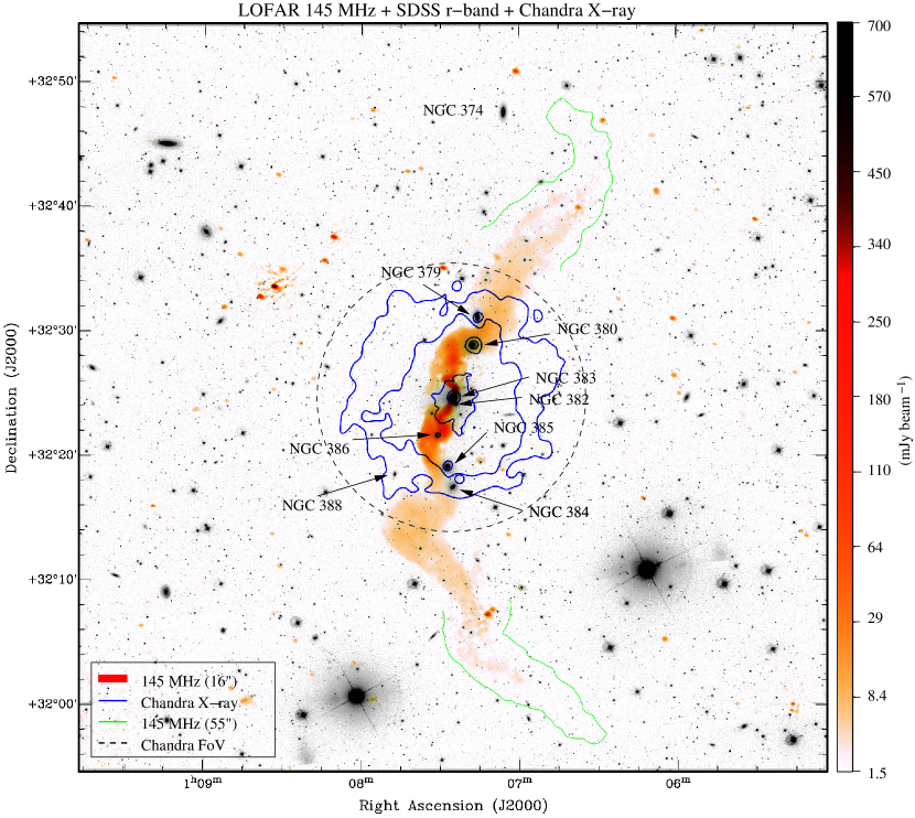
Figure 1: LOFAR 145-MHz radio continuum emission, overlaid on a SDSS r-band map with Chandra X-ray emission as contours. The image shows a $1~{}\rm deg^{2}$ area (corresponding to $1.2\times 1.2$ Mpc²), centred on 3C 31, where the 145-MHz radio continuum emission is shown with a red colour transfer function ($1.5\ldots 700~{}\rm mJy\,beam^{-1}$) at $16.5\times 11.8~{}\rm arcsec^{2}$ ($\rm PA=73\degr$) resolution. The blue contours show the hot gas of the ICM as traced by Chandra X-ray emission (contours at $0.7$, $0.84$, $1.2$ and $2.4$ ACIS counts s^-1), where the dashed circle indicates the FOV of the Chandra observations. Green contours indicate the maximum extent of the faint radio tails as measured from our low-resolution map (contours are at $4.5~{}\rm mJy\,beam^{-1}$).

As for the HBA observations, we performed the final imaging of the data within CASA, using the MS–MFS CLEAN algorithm with the spectral index fitting of the sky model enabled (‘nterms=2’) and a variety of angular scales. The rms noise of the LBA image is 5 $\rm mJy\,beam^{-1}$ using robust weighting (‘robust=0’) at a resolution of $38.0\times 23.5~{}\rm arcsec^{2}$ ($\rm PA=-73\degr$). The theoretical resolution is in good agreement (within 5 per cent) of the actual resolution, as for the LOFAR HBA data (Section 2.1).

2.3 VLA data

Observations with the Karl G. Jansky Very Large Array (VLA) with the recently commissioned $P$-band receiver were taken between 2013 December and 2014 December (see Table 1 for details). We followed standard data reduction procedures, using CASA and utilizing the flux scale by Scaife & Heald (2012). We checked that no inverted cross-polarizations were in the data (M. Mao & S. G. Neff 2014, priv. comm.). Of the 16 spectral windows 5 had to be discarded (1, 2, 11, 14 and 15) because the primary calibrator 3C 48 had no coherent phases, which prevents calibration. A further three spectral windows (0, 8 and 9) had to be flagged because of strong RFI. We imaged the data in CASA, first in A-array alone to self-calibrate phases, then in A- and B-array, and finally in A-, B- and C-array together. Prior to combination we had to change the polarization designation from circular polarizations (Stokes $RR$, $LL$) to linear polarization (Stokes $XX$, $YY$) of the A- and B-array data. Furthermore, we had to re-calculate the weights of the C-array data which were unusually high ($\approx$$10000$). We performed two rounds of self-calibration in phase only followed by two rounds of self-calibration in phase and amplitude with solution intervals of 200 s. We normalized the amplitude gains and found that the integrated flux densities of 3C 31 and 34 did not change by more than 2 per cent. The rms noise of the full bandwidth VLA $P$-band image is $0.15~{}\rm mJy\,beam^{-1}$ at a resolution of $7.5\times 4.6~{}\rm arcsec^{2}$ ($\rm PA=71\degr$). The largest angular scale the VLA can detect at 360 MHz is $1\aas@@fstack{\circ}1$ in C-array, which is enough to image 3C 31 to the same angular extent as measured with LOFAR.

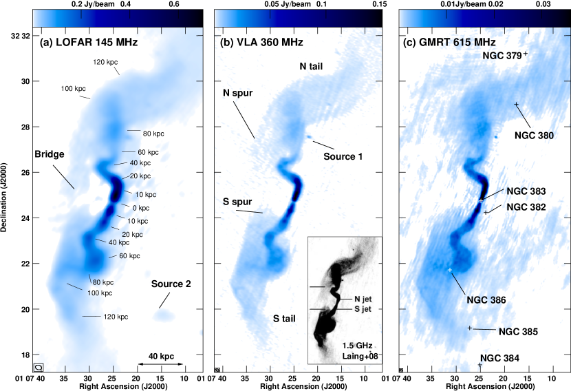
Figure 2: Left: Zoom-in on the combined LOFAR HBA data at 115–178 MHz, with a mean frequency of 145 MHz, at an angular resolution of $16.5\times 11.8~{}\rm arcsec^{2}$ ($\rm PA=73\degr$). The map shows the central 14 arcmin (290 kpc), centred on the nucleus. The transfer function ($1.5$–700 mJy beam^-1) is stretched to show weak, diffuse emission. The rms noise is approximately $0.5$ mJy beam^-1. Middle: Combined VLA data at 260–420 MHz (mean 360 MHz) at an angular resolution of $8.7\times 4.7~{}\rm arcsec^{2}$ ($\rm PA=71\degr$). The grey-scale corresponds to intensities of $0.05$–150 mJy beam^-1. The rms noise level is $0.25~{}\rm mJy\,beam^{-1}$. The inset shows the $1.5$-GHz map of Laing et al. (2008) at $5.5$ arcsec resolution. Right: Combined GMRT data at 615 MHz at an angular resolution of $5.4\times 4.5~{}\rm arcsec^{2}$ ($\rm PA=56\degr$). The grey-scale corresponds to intensities of $0.15$–36 mJy beam^-1. The rms noise level is $0.3~{}\rm mJy\,beam^{-1}$. In panels (a)–(c), we label features discussed in the text with the size of the synthesized beam shown in the bottom-left corner. Panel (c) shows the position of the cluster galaxies.

2.4 GMRT data

Observations with the Giant Metrewave Radio Telescope (GMRT) were taken in August 2007 in 615/235 MHz dual band mode (Swarup, 1991, see Table 1 for details). In this mode, the frequencies are observed simultaneously in two 16-MHz sub-bands consisting of $128\times 125$-kHz channels. The 615-MHz data are stored in one polarization ($RR$) in both the upper and lower sideband. The data reduction was carried out following standard flagging and calibration procedures in AIPS. The FWHM of the GMRT primary beam at 615 MHz is 44 arcmin; we corrected for primary beam attenuation in our final images with PBCOR (part of AIPS). In order to accurately recover the flux and structure of 3C 31, we imaged all bright sources well beyond the primary beam, using faceting to account for the sky curvature. The extent of 3C 31 is such that at 615 MHz, two facets were necessary to cover the entire source, one for each radio tail. The seam between the two facets was placed such that it crosses between the bases of the two jets where no radio emission is observed. The facets were iteratively CLEANed to reveal increasingly faint emission and then re-gridded on the same coordinate system and linearly combined with FLATN (part of AIPS) to create the final image. The GMRT 615-MHz map has a final synthesized beam of $5.4\times 4.5~{}\rm arcsec^{2}$ ($\rm PA=56\degr$) and the rms noise is $0.3$ mJy beam^-1.

2.5 General map properties

In addition to the new reductions described above, we used a $609$-MHz map observed with the Westerbork Radio Synthesis Telescope (WSRT), which we obtained from the ‘Atlas of DRAGNs’ public webpage which presents 85 objects of the ‘3CRR’ sample of Laing et al. (1983). This map, which was presented by Strom et al. (1983), has an angular resolution of 55 arcsec, the lowest of our 3C 31 maps. The WSRT 609-MHz map has the advantage over the GMRT 615-MHz map that it recovers better the large-scale structure of 3C 31, which is largely resolved out in the high-resolution GMRT map. Hence, for the spectral analysis in what follows we use only the WSRT 609-MHz map while the GMRT 615-MHz map is used only for the morphological analysis. The maps created from the LOFAR and VLA observations, together with the WSRT map, will be used in the rest of the paper to study the spatially resolved radio spectral index of 3C 31.

In order to ensure that we have a set of maps that are sensitive to the same angular scales, we imaged all our data with an identical $(u,v)$-range between $0.04$ and $4.9$ k$\lambda$. Since we did not have the the $(u,v)$ data for the 609-MHz map available, we could not re-image these data. But the $(u,v)$-range for these data is with $0.06\rightarrow 5.6~{}{\rm k}\lambda$ quite similar, so re-imaging is not necessary. In what follows, these maps are referred to as ‘low-resolution maps’, whereas the maps without a $(u,v)$-range applied are referred to as ‘full-resolution maps’.

For further processing, we took the maps into AIPS, where we made use of PYTHON scripting interface PARSELTONGUE (Kettenis et al., 2006) to batch process them. We used CONVL to convolve them with a Gaussian to the same angular resolution and HGEOM to register them to the same coordinate system. To create a mask, we blanked unresolved background sources with BLANK, and applied the same mask to all maps to be compared. The flux densities as determined from the final maps are in agreement with literature values. The integrated spectrum of 3C 31 can be described by a power law between $30$ and $10700$ MHz with a radio spectral index of $-0.67\pm 0.01$. We use calibration uncertainties of 5 per cent and add noise contributions from the rms map noise and zero-level offset in order to determine our uncertainties (see Appendix A for details).

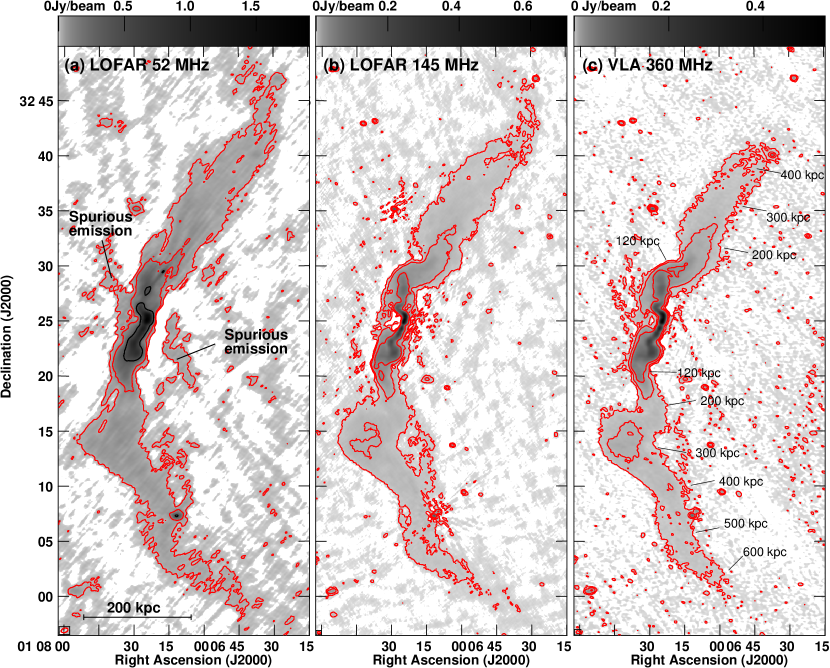
Figure 3: Left: Combined LOFAR LBA data at 35–85 MHz (mean 52 MHz), at an angular resolution of $38.0\times 23.5~{}\rm arcsec^{2}$ ($\rm PA=-73\degr$). The transfer function (0–1900 mJy beam^-1) is stretched to show weak, diffuse emission. The rms noise is $6.5$ mJy beam^-1. Middle: Combined LOFAR HBA data at 115–178 MHz (mean 145 MHz), at an angular resolution of $16.5\times 11.8~{}\rm arcsec^{2}$ ($\rm PA=73\degr$). The grey-scale corresponds to intensities of 0–700 mJy beam^-1. The rms noise is $0.5~{}\rm mJy\,beam^{-1}$. Right: Combined VLA $P$-band data at 288–432 MHz (mean 360 MHz), at an angular resolution of $21.0\times 14.6~{}\rm arcsec^{2}$ ($\rm PA=74\degr$). The grey-scale corresponds to intensities of 0–530 mJy beam^-1. The rms noise level is $0.3~{}\rm mJy\,beam^{-1}$. In all panels, contours are at $2.5$, $12.5$ and $62.5$ $\times$ the rms noise level and the size of the synthesized beam is shown in the bottom-left corner.

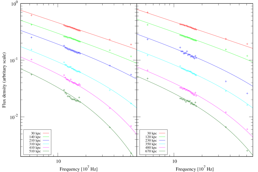
Figure 4: Radio continuum spectra within selected regions between 52 and 609 MHz at 20 frequencies (LOFAR LBA 52 MHz, 17 combined sub-bands at 117–173 MHz from LOFAR HBA, VLA 360 MHz and WSRT 609 MHz). Solid lines are the spectra as predicted by our best-fitting advection models. The size of the data points is approximately equivalent to the size of the error bars. Spectra in the northern tail are shown in the left panel, spectra in the southern tail are shown in the right panel. The legend shows the distance to the nucleus (see Figs. 2c and 3c).

3 Morphology and observed spectrum

3.1 Morphology

Figure 1 presents a panoramic low-frequency view of 3C 31, showing our 145-MHz map at full resolution as colour-scale, with contours of Chandra X-ray emission, showing the hot ICM. We overlay the data on a SDSS r-band image, which shows the optical stellar light. The SDSS r-band image shows the large, diffuse halo of the host galaxy, NGC 383, with a diameter of 3 arcmin (60 kpc). The closest member of the group is NGC 382, $0.5$ arcmin (10 kpc) south-south-west of NGC 383. There are a handful of further members of this group, some of which can be detected in the X-ray data as point-like sources embedded in the diffuse X-ray emission from the ICM. None shows any radio emission in our image.

Figure 2 shows the full-resolution maps of the central 14 arcmin (290 kpc) at 145 (LOFAR HBA), 360 (VLA) and 615 MHz (GMRT). Our 360-MHz map shows the northern and southern ‘spurs’ of Laing et al. (2008) – extensions from the tails towards the nucleus. Both spurs are also visible in the 145-MHz map, where the northern spur is connected via a ‘bridge’ to the southern one. Similarly, the 615-MHz map shows both spurs although the visibility of the northern one is limited by the image fidelity. We find two compact sources in the radio continuum near the jet (labelled as ‘Source 1’ and ‘Source 2’ in Fig. 2), but they have no counterparts in the optical (SDSS), the mid-infrared (WISE 22 $\mu$m; Wright et al., 2010) or in the far-UV (GALEX). We thus conclude that these sources are unrelated to 3C 31 or the galaxies associated with it.

Further away from the nucleus, the radio tails can be particularly well traced at low frequencies. Figure 3 presents our maps at full resolution (although we omit the A-array from the VLA data) at 52 (LOFAR LBA), 145 (LOFAR HBA) and 360 MHz (VLA); the emission extends spatially further than any of the previous studies have revealed. Andernach et al. (1992) found an angular extent of 40 arcmin in declination in their 408-MHz map and speculated that the tails did not extend any further. Our new data show that 3C 31 extends at least 51 arcmin mostly in the north-south direction, between declinations of $+31\degr 57\arcmin$ and $+32\degr 48\arcmin$, as traced by our most sensitive 145-MHz map. The projected linear size hence exceeds 1 Mpc, so that 3C 31 can now be considered to be a member of the sub-class of objects that are referred to in the literature as giant radio galaxies (GRGs). It remains difficult to ascertain whether we have detected the full extent of 3C 31 since it is certainly possible that the radio emission extends even further, as 3C 31 has tails of diffuse emission extending away from the nucleus – as opposed to lobes with well-defined outer edges (see de Gasperin et al., 2012, for a LOFAR study of Virgo A, exhibiting well-defined lobes).

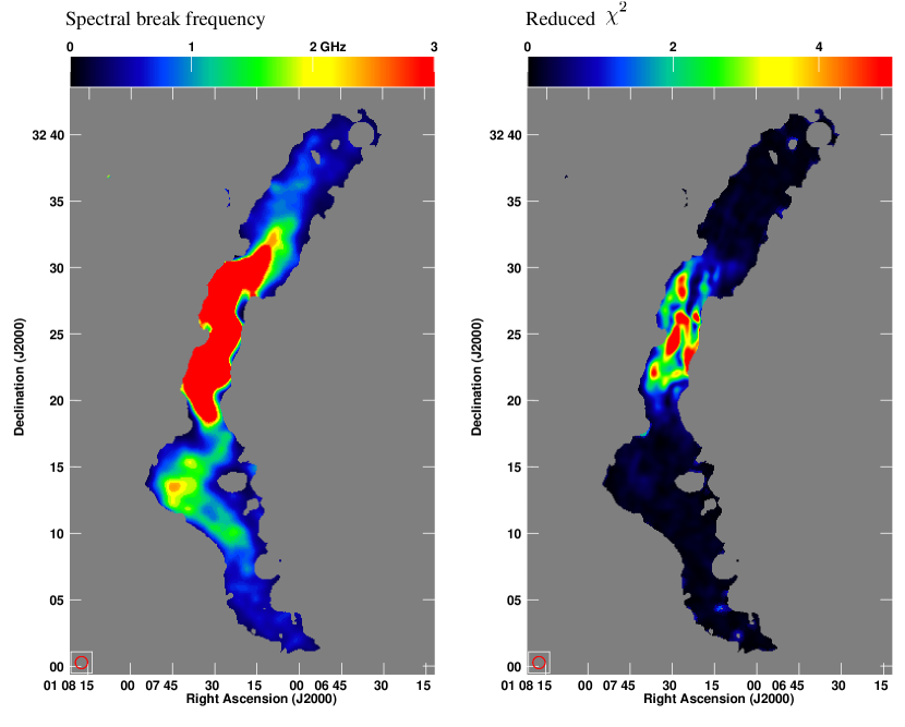
Figure 5: Left: Spectral break frequency at 55 arcsec angular resolution (equivalent to 19 kpc) as indicated by the boxed circle in the bottom-left corner. Data points at 20 frequencies (LOFAR LBA 52 MHz, 17 combined sub-bands at 117–173 MHz from LOFAR HBA, VLA 360 MHz and WSRT 609 MHz) were fitted with a JP model (assuming $\delta_{\rm inj}=2.1$). Right: The corresponding reduced $\chi^{2}$.

Weżgowiec, Jamrozy & Mack (2016) claimed the detection of diffuse $1.4$-GHz emission surrounding 3C 31, based on combining NVSS and Effelsberg single-dish imaging data. Their integrated flux density of 3C 31 lies $\approx$$1.2$ Jy (or $3.6~{}\sigma$) above our integrated power-law spectrum (see Appendix A), which predicts a $1.4$-GHz flux density of $5.61$ Jy. We find no hint of this ‘halo’ structure. The largest detectable angular scale in our HBA map is $\approx$$1\aas@@fstack{\circ}4$ (a factor $1.6$ larger than the detected total source extent), so that we should not be resolving out cocoon structure on scales comparable to the detected source. Our 145-MHz low-resolution map has a $3\sigma$ threshold in surface brightness of $\approx$$1.3~{}\mu$Jy arcsec^-2. If we consider the 1.4-GHz extended halo feature reported by Weżgowiec et al. (2016) and assume a halo flux of $\approx$$1.2$ Jy (the excess emission above our integrated spectrum) distributed uniformly over a surface area of $\approx$$227$ arcmin², then for $\alpha$ between $-0.7$ and $-1.5$, the 145-MHz surface brightness would be between $7$–$45~{}\mu$Jy arcsec^-2. This is well above our detection threshold, and even bearing in mind the likely uncertainty in the flux estimate from Weżgowiec et al. (2016), our data are not consistent with the presence of the large-scale halo presented in that work. However, we cannot rule out the existence of an even larger, lower surface brightness halo, which could still evade detection in our observations. This possibility is discussed in Section 5.2.

3.2 Spectrum

In Fig. 4, we show the evolution of the radio continuum spectrum as function of distance from the nucleus. The spectrum is a power law within 120–140 kpc from the nucleus, so that spectral ageing plays no role there, at least not in the frequency range covered by our data. At larger distances, a significant spectral curvature develops, which grows with increasing distance from the nucleus. The spectra can be characterized by the fitting of Jaffe–Perola (JP; Jaffe & Perola, 1973) models to determine a characteristic (‘break’) frequency (e.g. Hughes, 1991). We fitted models to our low-resolution maps using the Broadband Radio Astronomy Tools (BRATS; Harwood et al., 2013), assuming a CRE injection spectral index of $\delta_{\rm inj}=2.1$ (with a CRE number density of $n\propto E^{-\delta_{\rm inj}}$, where $E$ is the CRE energy). The resulting spectral break frequency is shown in Fig. 5. The high reduced $\chi^{2}$ found in the inner region can be at least in part explained due to averaging over regions with very different spectra (cf. fig. 12 in Laing et al., 2008). We used for the fitting 17 combined sub-bands from LOFAR HBA, but we tested that using only one HBA map instead changes the spectral age locally by 20 per cent at most and averaged across the tails the difference is even smaller.

As expected, the spectral break frequency decreases with increasing distance from the nucleus, which can be explained by spectral ageing. The spectral break frequency $\nu_{\rm brk}$ can be related to the age $\tau_{\rm Myr}$ of the CREs (in units of Myr) via (e.g. Hughes, 1991):

$$\nu_{\rm brk}=2.52\times 10^{3}\frac{B/{10~{}\mu\rm G}}{[(B/{10~{}\mu\rm G})^{2}+(B_{\rm CMB}/{10~{}\mu\rm G})^{2}]^{2}\tau_{\rm Myr}^{2}}~{}{\rm GHz},$$ (1)

where $B$ is the magnetic field strength and $B_{\rm CMB}$, the equivalent cosmic microwave background (CMB) magnetic field strength of $3.2~{}\mu\rm G$ (at redshift zero), is defined so that the magnetic energy density is equal to the CMB photon energy density. If we use a magnetic field strength of $B=5~{}\mu\rm G$, which is an extrapolation from CH14, we find that for a spectral break frequency of 1 GHz, the CREs are 100 Myr old. This already provides a good estimate of the source age. However, the magnetic field strength (whether estimated via equipartition or otherwise) is expected to change with distance from the nucleus, and the average field strength may be different to the value we assume here. In the next section, we introduce a model of cosmic-ray transport in order to investigate the evolution of tail properties in more detail.

4 Cosmic-ray transport

To explore the tail physical conditions and dynamics in more detail we use the quasi-1D cosmic-ray transport model of Heesen et al. (2016, hereafter HD16). In that work, cosmic-ray transport via advection and diffusion is considered within galaxy haloes. For a jet environment we expect advection to be the dominant transport mode. This is corroborated by the intensity profiles, which are of approximately exponential shape as expected for an advection model (HD16) and the corresponding radio spectral index profiles, which show a linear steepening (Fig. 6).

The model self-consistently calculates the evolution of the CRE spectrum along the tails, accounting for adiabatic, synchrotron and inverse Compton (IC) losses, with the aim of reproducing the evolution of radio intensity and spectral index, as shown in Fig. 6. The aim is to obtain a self-consistent model for the velocity distribution and the evolution of magnetic field strength along the tails. We make the following basic assumptions: (i) the tail is a steady-state flow, (ii) the CRE energy distribution is described by a power law at the inner boundary, and (iii) there is no in-situ particle acceleration in the modelled region. The first assumption is not strictly valid in the outermost parts of the source, as we expect that the tails are still growing; we discuss the effects of expansion of the outer tails in Section 4.4. The second assumption is well justified by the radio spectral index in the inner jet (Fig. 4). It is difficult to obtain any direct constraints on particle acceleration in the outer parts of FR I plumes, and so the assumption of no particle acceleration is a limitation of all spectral ageing models.

We model the tails between 15 kpc and 800 (northern) or 900 (southern tail) kpc, taking 15 kpc as the inner boundary, as the jet parameters at this distance are well constrained from the work of Laing & Bridle (2002a, b). The geometry of the tails is taken from observations assuming a constant inclination angle of $52\degr$ to the line of sight (Laing & Bridle, 2002a). The details of the advection modelling process are described in Section 4.2. There are a number of free parameters in the model, and so in the next section we summarize our approach to exploring the parameter space of possible models.

4.1 Modelling approach and assumptions

The model parameters are as follows, where the injection parameters are at 15 kpc distance from the nucleus:

• Injection magnetic field, $B_{0}$

• Injection velocity, $\varv_{0}$

• The deceleration parameter, $\beta$

with the primary model outputs being a profile of velocity and magnetic field strength along the tail. The expansion of the tails leads to strong adiabatic losses along the tail which are inconsistent with the observed spectral evolution unless the flow is decelerating. We chose to model such a deceleration assuming $\varv\propto r^{\beta}$, where $r$ is the tail radius. We also tested a velocity dependence on distance rather than tail radius; however, this led to poorer model fits. The dependence on radius would be expected from momentum flux conservation if mass entrainment is occurring in regions where the radius increases (e.g. CH14). We assumed $\delta_{\rm inj}=2.1$, consistent with the work of Laing & Bridle (2002a) and our observed spectra in the inner parts of the source (Appendix A).

Our modelling approach then involves considering a range of input values for $\beta$, $\varv_{0}$ and $B_{0}$, and applying the advection model as described in Section 4.2 below to determine an output magnetic field and velocity profiles $B(z)$ and $\varv(z)$ (where $z$ is distance along the tail) that minimize $\chi^{2}$. However, there is an intrinsic degeneracy between the velocity and magnetic field strength profiles along the tail if we wish to avoid the traditional minimum energy assumption in which the CRE and magnetic field energy densities are approximately equal with no relativistic protons. Hence there are multiple combinations of parameters that can achieve a good fit to the radio data.

Our initial approach to tackling the degeneracy between velocity and magnetic field strength is to compare the best-fitting magnetic field profiles for a range of input parameters ($\beta$, $\varv_{0}$, $B_{0}$) with the expected magnetic field strength profile of models that use further observational constraints – specifically, assuming pressure equilibrium with the surrounding X-ray emitting ICM (e.g. CH14) – in order to assess their physical plausibility. In Section 4.4, we also discuss alternative scenarios.

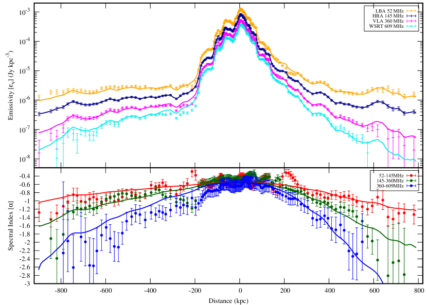
Figure 6: Top panels: Profiles of the radio continuum emissivity as function of distance from the nucleus at various frequencies. Shown are the LOFAR LBA 52 MHz (orange), HBA 145 MHz (dark blue), VLA 360 MHz (magenta) and WSRT 609 MHz (cyan) observations. Bottom panels: Corresponding profiles of the radio spectral index between 52 and 145 MHz (red), 145 and 360 MHz (dark green) and between 360 and 609 MHz (blue). Solid lines show the best-fitting advection models using SPINNAKER (see text for details). The northern tail is on the right-hand side ($z>0$ kpc) and the southern tail is on the left-hand side ($z<0$ kpc).

4.2 Advection model

Our quasi-1D cosmic-ray transport model (based on HD16) is able to predict non-thermal (synchrotron) radio continuum intensity profiles at multiple frequencies, assuming advection is the dominant transport process. For no in-situ cosmic-ray acceleration in the tails, the stationary (no explicit time dependence) advection model prescribes the CRE flux (units of $\rm s^{-1}\,GeV^{-1}$) $N(E,z)$ as:

$$\frac{\partial N(E,z)}{\partial z}=\frac{1}{\varv}\left[\frac{\partial}{\partial E}\left(b(E)N(E,z)\right)\right]\qquad(z>0),$$ (2)

where $z$ is distance along the tail, $E$ is the electron energy, $\varv$ is the advection speed (which may depend on position) and $b(E)$ include the losses of the CREs via IC and synchrotron radiation as well as adiabatic losses:

$$b(E) = -\left(\frac{{\rm d}E}{{\rm d}t}\right)=-\left(\frac{{\rm d}E}{{\rm d}t}\right)_{\rm IC}-\left(\frac{{\rm d}E}{{\rm d}t}\right)_{\rm syn}-\left(\frac{{\rm d}E}{{\rm d}t}\right)_{\rm ad}$$

$$= \frac{4}{3}\sigma_{\rm T}c\left(\frac{E}{m_{\rm e}c^{2}}\right)^{2}U_{\rm rad}+\frac{4}{3}\sigma_{\rm T}c\left(\frac{E}{m_{\rm e}c^{2}}\right)^{2}U_{\rm B}+\frac{E}{t_{\rm ad}},$$

where $U_{\rm rad}=4.2\times 10^{-13}~{}\rm erg\,cm^{-3}$ is the radiation energy density (here the only source is the CMB), $U_{\rm B}=B^{2}/(8\pi)$ is the magnetic energy density, $\sigma_{\rm T}=6.65\times 10^{-25}~{}\rm cm^{2}$ is the Thomson cross section and $m_{\rm e}=511~{}\rm keV\,c^{-2}$ is the electron rest mass. Adiabatic losses are caused by the longitudinal dilution of the CRE density due to an accelerating flow or due to lateral dilution by an expanding flow. The corresponding losses of the CREs is ${\rm d}E/{\rm d}t=-1/3(\nabla\varv)E$ (Longair, 2011). This means we can calculate the adiabatic loss time-scale as (Appendix B):

$$t_{\rm ad}=\frac{3}{2}\left(\frac{\varv}{r}\cdot\frac{\partial r}{\partial z}\right)+3\frac{\partial\varv}{\partial z},$$ (4)

where $r$ is the tail radius. In HD16, $N(E,z)$ describes the CRE number density, which is identical to the CRE flux when the advection velocity and cross-sectional areas are constant. In our case, however, we need to convert the CRE flux into the CRE number density (units of $\rm cm^{-3}\,GeV^{-1}$):

$$n=\frac{N}{A\cdot\varv}.$$ (5)

Then, the model emissivity can be calculated with the following expression using $A=\pi r^{2}$:

$$\epsilon_{\nu}={\rm const.}\int_{0}^{\infty}j(\nu)\frac{N(E,z)}{r^{2}\varv}{\rm d}E,$$ (6)

where $j(\nu)={\rm(const.)}B(z)F(\nu)$ is the synchrotron emissivity of a single ultra-relativistic CRE (Rohlfs & Wilson, 2004). Here, we have assumed a uniform distribution of the CRE number density and that the tails are cylindrical over small ranges of distances from the nucleus $\Delta z$. Now, we determine the observed emissivity profiles. The emissivity $\kappa_{\nu}$ of a small volume in the tails can be calculated in a straightforward way as:

$$\kappa_{\nu}=\frac{S_{\nu}}{\pi r^{2}\Delta z},$$ (7)

where $\pi r^{2}\Delta z$ is the volume from which the emission stems, noting that $z$ is the physical distance from the nucleus. In order to convert the observed intensities into emissivities, we first calculate the flux density of the emitting volume:

$$S_{\nu}=\langle I_{\nu}\rangle\cdot\frac{2r\Delta z\cdot\sin(\vartheta)}{\Omega\cdot D^{2}},$$ (8)

where $\langle I_{\nu}\rangle$ is the average intensity across the integration area, $\vartheta=52\degr$ is the inclination angle of the tail to the line of sight and $\Omega$ is the solid angle of the synthesized beam. We measure the radius $r$ of the tails from our 145-MHz low-resolution map and from our 360-MHz full-resolution map in the inner part. Then, the emissivity is:

$$\kappa_{\nu}=\langle I_{\nu}\rangle\cdot\frac{2\cdot\sin(\vartheta)}{\pi r\Omega\cdot D^{2}}.$$ (9)

Combining all the constants and retaining only the variables, we find for the observed emissivity:

$$\kappa_{\nu}=1.16\times 10^{-3}\cdot\frac{\langle I_{\nu}\rangle}{r/{\rm kpc}}~{}{\rm Jy\,kpc^{-3}},$$ (10)

The observed emissivity profiles are shown in Fig. 6.

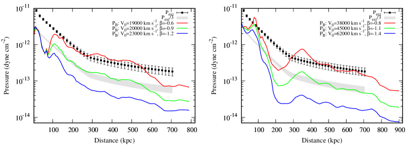
Figure 7: Comparison of the external pressure $P_{\rm ext}$ (data points) with the magnetic pressure $P_{\rm B}$ in the northern (left) and southern tail (right). The grey-shaded area indicates the range of pressures if the external pressure, extrapolated beyond the observed profile of CH14 extending to $\approx$$200$ kpc using their best-fitting model, is divided by a constant factor of $3$, which is the expected magnetic pressure for the entrainment model of CH14 (see text for details). The various lines are the best-fitting advection models for Model I ($B_{0}=15~{}\mu\rm G$) and for various values of $\beta$.

Table 2: Results of the cosmic-ray transport modelling.

Parameter	Northern tail	Southern tail
Injection spectral index ($\delta_{\rm inj}$)	$2.1$
Deceleration ($\beta$, $\varv\propto r^{\beta}$)	$-0.9$	$-1.1$
Degrees of freedom ($\rm dof$)	83	67
— Model I: $B_{0}$ from CH14 entrainment model —
Injection magnetic field ($B_{0}$)	$15~{}\mu\rm G$
Injection velocity ($\varv_{0}$)	$20000~{}\rm km\,s^{-1}$	$45000~{}\rm km\,s^{-1}$
Advection time ($\tau_{\rm adv}$)	190 Myr	160 Myr
Reduced $\chi^{2}$	$1.3$	$1.6$
— Model II: $B_{0}$ assuming magnetically dominated tails —
Injection magnetic field ($B_{0}$)	$26~{}\mu\rm G$
Injection velocity ($\varv_{0}$)	$40000~{}\rm km\,s^{-1}$	$80000~{}\rm km\,s^{-1}$
Advection time ($\tau_{\rm adv}$)	100 Myr	90 Myr
Reduced $\chi^{2}$	$1.3$	$1.7$
— Model III: $B_{0}$ assuming equipartition and no relativistic protons —
Injection magnetic field ($B_{0}$)	$9~{}\mu\rm G$
Injection velocity ($\varv_{0}$)	$13000~{}\rm km\,s^{-1}$	$31000~{}\rm km\,s^{-1}$
Advection time ($\tau_{\rm adv}$)	300 Myr	240 Myr
Reduced $\chi^{2}$	$1.6$	$1.4$

HD16 developed the computer code SPINNAKER (SPectral INdex Numerical Analysis of K(c)osmic-ray Electron Radio-emission), which implements the methods discussed above to model the radio continuum emission. The right-hand side of equation (2) is solved numerically using the method of finite differences on a two-dimensional grid, which has both a spatial and a frequency (equivalent to the CRE energy) dimension. The left-hand side of equation (2) can then be integrated from the inner boundary using a Runge–Kutta scheme (e.g. Press et al., 1992), which provides us with a profile of $N(E,z)$. The initial parameters (see Section 4.1) are listed in Table 2.

4.3 Fitting procedure

For each set of input parameters ($B_{0}$, $\varv_{0}$, $\beta$), we used SPINNAKER to fit equation (6) to the observed radio emissivity profiles obtained from equation (10). We fit only to the 145-MHz data within distances $z<140~{}\rm kpc$ (in the northern tail) and $|z|<360$ kpc (in the southern tail) because the spectral index in this area becomes unreliable due to insufficient angular resolution (resulting in a superposition of different CRE populations), but include the other three radio frequencies beyond these distances. The reduced $\chi^{2}_{\rm red}$ is:

$$\chi^{2}_{\rm red}=\frac{1}{\rm dof}\sum\left(\frac{\kappa_{\nu,i}-\zeta\cdot{\epsilon_{\nu,i}}}{\sigma_{i}}\right)^{2}.$$ (11)

Here, $\kappa_{\nu,i}$ is the $i$th observed emissivity and $\epsilon_{\nu,i}$ the corresponding model emissivity, $\sigma_{i}$ the error of the observed value and $\rm dof$ is the degree of freedom (number of data points minus number of fitting parameters). The normalization parameter $\zeta$ is determined by minimizing the reduced $\chi^{2}$. The magnetic field is then varied with an iterative process where the 145-MHz observed emissivities are fitted, assuming that the model emissivities scale as $\epsilon_{\nu}\propto B^{1-\alpha}$. If the magnetic field has to be adjusted locally, the field has to change as $B\propto\epsilon_{\nu}^{1/(1-\alpha)}$ (which is accurate if $N(E,z)$ follows a power law in energy):

$$B_{j+1}(z)=B_{j}(z)\times\left(\frac{\kappa_{145}(z)}{\xi\cdot[\epsilon_{145}(z)]_{j}}\right)^{1/(1-\alpha_{52-145})},$$ (12)

where $\alpha_{52-145}$ is the radio spectral index between 52 and 145 MHz. This is repeated several times until the fit converges and the reduced $\chi^{2}$ does not decrease any further. Here, $j$ is an integer variable, describing consecutive magnetic field models. While fitting equation (12), we vary the normalization factor of the model emissivities $\xi$ so that $B_{0}$ is unchanged. In summary, the procedure is as follows:

1. Prescribe the magnetic field strength profile.

2. Fit the model, deriving the scaling $\zeta$ by minimize the reduced $\chi^{2}$ (equation 11).

3. Adjust the magnetic field profile using equation (12), varying $\xi$ so that $B_{0}$ is fixed.

4. Iterate (ii) and (iii) until $\chi^{2}$ converges.

With this procedure the 145-MHz emissivities are perfectly fitted since all the variations in the profile are absorbed by the magnetic field profile. The real test for our model is that the other frequencies are fitted as well, hence the spectral index profiles are most important.

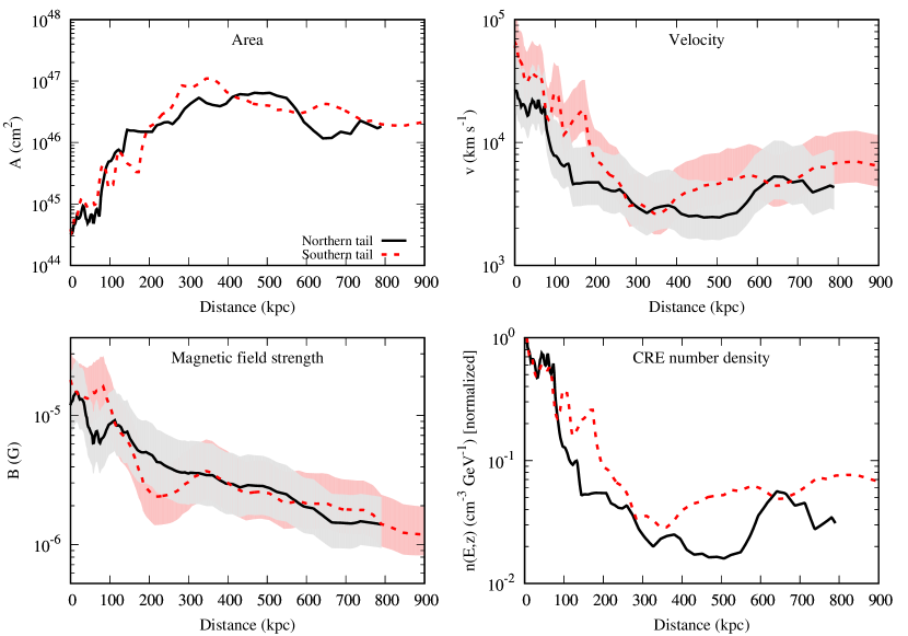
Figure 8: Cross-sectional area (top left), velocity (top right), magnetic field strength (bottom left) and CRE number density corresponding to a critical frequency of 145 MHz (bottom right) as function of distance to the nucleus. Profiles in the northern (southern) tail are shown as black solid (red dashed) lines, which are for Model I. The shaded areas indicate the variation of velocity and magnetic field strength when using Models II and III.

4.4 Results

Table 2 lists the model fitting results for three scenarios. In each case, we fixed $B_{0}$ and $\beta$, as explained below, and then determined the best-fitting magnetic field profile and $\varv_{0}$.

For our primary model (Model I in Table 2), we require the tail to be in rough pressure balance with the external medium, as measured by CH14. In their favoured model of dominant thermal pressure from entrained material, it was assumed that the magnetic field energy density is in rough equipartition with the total particle energy density. This model predicts that the magnetic field pressure contribution, $P_{\rm B}$, relates to the external pressure, $P_{\rm ext}$, as $P_{\rm B}=P_{\rm ext}/3$. In Fig. 7, we show the external pressure profile inferred from the measured profile of CH14, which extends to $\approx$$200$ kpc, extrapolating their best-fitting double-beta model to 700 kpc. The grey-shaded area indicates the predicted magnetic field pressure evolution in this model.

The magnetic field profile is almost solely determined by the profile of the velocity along the radio tails, due the strong effect of adiabatic losses on the evolution of CRE number densities. In Fig. 7 we show the effect of varying $\beta$ on the magnetic pressure profile: the best agreement with the extrapolated pressure profile of CH14 is for a value of $\beta\approx-1$. If we now vary the initial magnetic field strength $B_{0}$ but keep $\beta=-0.9$ (northern tail) and $\beta=-1.1$ (southern tail), the curves in Fig. 7 will move up and down, and the corresponding best-fitting $\varv_{0}$ values will change, but the magnetic pressure profile shape does not change. Table 2 compares the results of three models: Model I, using $B_{0}=15~{}\mu$G, taken from CH14, Model II in which the tails are magnetically dominated and the magnetic pressure is roughly equal to the external pressure, which corresponds to the most extreme high-$B$ scenario, and Model III, in which we assume that $B_{0}$ is the equipartition magnetic field assuming no relativistic protons. We used the magnetic field distribution indicated by the shaded area in Fig. 7 (Model I) as an initial guess and calculated the predicted radio intensities. For Models II and III, we rescaled this magnetic field profile to obtain the corresponding value of $B_{0}$. We can be confident that the true magnetic field pressure is somewhere in between these extremes. We have tested other starting conditions, e.g. uniform and exponential magnetic field profiles, and find that the final profiles of velocity and field strength after iteration are reasonably independent of the initial field strength profile for a given value of $\beta$. The best-fitting profiles are shown in Fig. 8, with the range allowed for the three models showed by the shaded areas. The corresponding best-fitting parameters are shown in Table 2.

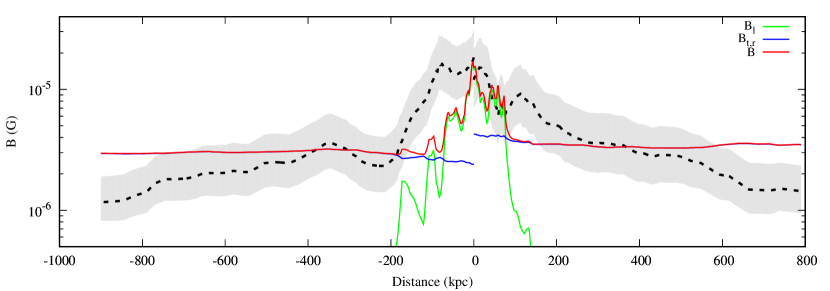
Figure 9: Adiabatic (flux conserving) magnetic field models. The black dashed line shows the best-fitting magnetic field strength from Model I, where the shaded area indicates the variation when using Models II and III. The green and blue lines denote the best-fitting longitudinal and toroidal (radial) model components and the red line the total field strength. The northern tail is on the right-hand side ($z>0$ kpc) and the southern tail is on the left-hand side ($z<0$ kpc).

We find that our models describe the data reasonably well, with a reduced $\chi^{2}\approx 1.5$. The spectral index profiles (Fig. 6, bottom panel) show a continuous decrease (steepening of the spectrum) with increasing slope with distance. Notably, the shape of the spectral index profiles is modelled accurately and has the typical shape of advective transport, where the spectral index steepens in almost linear way with only a slightly increasing curvature (cf. fig. 5 in HD16).

The resulting advection time-scale lies between 90 and 300 Myr. Our best-fitting velocity on scales exceeding $100$ kpc is broadly consistent with the estimated mean velocity of Andernach et al. (1992), based on data of considerably lower resolution and sensitivity. Our model assumes a steady-state flow, even in the outer parts of the tails, although in reality the tails are expected to be expanding in the longitudinal direction (the cylindrical shape in the outer few 100-kpc supports the assumption that the tails are not laterally expanding). We considered the effects of this growth on our assumptions, by comparing the time-scales for tail growth and advection of particles through the tails in the outer few 100-kpc. Since the cross-sectional area and the advection speed are both roughly constant in this region (Fig. 8), the fractional change in the length of a tail segment during the particle advection time-scale across that region is given by the ratio of the tail-tip advance speed and the advection speed. From ram-pressure balance (using the external pressure inferred from Fig. 7), which is an extrapolation from the inner model at the distance of interest, we estimate the tail-tip advance speed to be $\approx$$200~{}\rm km\,s^{-1}$, while the advection speed in the outer few 100-kpc is $\approx$$5000~{}\rm km\,s^{-1}$. Therefore the fractional increase in volume for a segment of jet over the particle advection time-scale is $\approx$4 per cent. As discussed in Section 3, it is likely that we are not detecting the full extent of the radio structure, and our external pressure estimate comes from an extrapolation rather than direct measurement at this distance. Consequently, the external pressure at the true end point of the source may be lower. However, the weak dependence of the advance speed on the external pressure means that this does not change the calculation very much for plausible environmental pressures. We conclude that the effect of tail growth on the particle energy evolution in the outer few 100-kpc should not significantly alter our results.

5 Discussion

5.1 Magnetic field structure

What regulates the magnetic field strength in the radio tails? One possibility is simply that flux conservation is responsible. In cylindrical coordinates, with the $z$-axis along the tail, the magnetic field has a longitudinal component $B_{\rm l}$ and two transverse components, a radial $B_{\rm r}$ and a toroidal $B_{\rm t}$ one. As Laing & Bridle (2014) have shown, the magnetic field in FR I jets to first order makes a transition from longitudinal (first few kpc, where the jet is relativistic) to toroidal, occasionally with a significant radial component. From flux conservation it is expected that the longitudinal component falls much more rapidly than the two transverse components because for a 1D non-relativistic flow (Baum et al., 1997):

$$\begin{array}[]{ll}B_{\rm l}\propto r^{-2}\quad{\rm(longitudinal)}\\[5.0pt] B_{\rm t},~{}B_{\rm r}\propto(r\varv)^{-1}=r^{-1-\beta}\quad{\rm(toroidal,radial)},\end{array}$$ (13)

where $r$ is the tail radius and $\varv$ the advection velocity. While we expect the radial component to fall off rapidly with radius with $B_{l}\propto r^{-2}$, the toroidal and radial components should be almost constant if $\beta\approx-1$. We have fitted these models to our recovered magnetic field distribution (Fig. 8), using the following normalization:

$$B=B_{0}\cdot\left[f^{2}\cdot\left(\frac{A}{A_{0}}\right)^{-2}+(1-f^{2})\cdot\left(\frac{A}{A_{0}}\right)^{-1-\beta}\right]^{0.5},$$ (14)

where $A_{0}$ is the cross-sectional area of the tail and $f$ is the ratio of longitudinal to total magnetic field strength at $|z|=15$ kpc. The resulting flux-freezing magnetic field models are shown in Fig. 9. At injection, the best-fitting flux conservation scenario requires that the longitudinal magnetic field component totally dominates and the radial and toroidal field strengths are very small. At distances $>$100 kpc from the nucleus, the longitudinal component becomes rapidly negligible compared with the toroidal and radial magnetic field components. However, the flux-freezing models do not fit the observed magnetic field profile very well. At best, our advection model results are consistent with such a flux conservation model out to a distance of $\approx$500 kpc. At larger distances, magnetic flux cannot be conserved as the resulting magnetic field pressure becomes too high. It is clear from the relatively flat profiles of cross-sectional area and velocity shown in Fig. 8 that the magnetic field evolution should be roughly constant if flux is conserved, whereas our model, strongly constrained by the observations, implies a decreasing magnetic field strength with distance. We note that similar geometrical arguments apply to the model of CH14 so that flux freezing is not consistent with the evolution of the inner plumes in their model. An alternative scenario is that the magnetic flux evolution is affected by entrainment, either continuously along the tails or at particular locations where some level of disruption occurs, with energy transferred between the magnetic field and evolving particle population.

5.2 Source age and energetics

An important characteristic of radio galaxies is the source age, which can be measured either as a dynamical time-scale if the source expansion speed is known, or as a spectral time-scale derived from the spectral ageing of the CREs (e.g. Heesen et al., 2014). We can use the sound crossing time as a first estimate for the source age (Wykes et al., 2013). The ICM temperature is approximately $1.5$ keV (CH14, their table 1), resulting in a sound speed of $600~{}\rm km\,s^{-1}$, implying a sound crossing time of $\approx$$1000$ Myr. This would provide an upper limit to the source age were we confident about the inclination of the outer tails, but if the outer parts are more projected than we assume based on the inner jet, the true sound-crossing time could be higher. If, instead, we assume that we are observed the oldest plasma in the outer parts of the tails, then we obtain a source age of $\approx$$200$ Myr. If our advection time-scale gives a realistic estimate of the source age, then the average source expansion speed is $\approx$$5$ times the speed of sound. As discussed in Section 4.4, ram-pressure balance arguments suggest that the current expansion speed is considerably lower than this, so that the overall source expansion at the present time is not supersonic. This apparent inconsistency could be explained if there is a weak internal shock somewhere beyond the detected emission, with back-flowing material forming an undetected cocoon of older plasma. If no such cocoon of material exists, then the advection speeds found by our model must be too high, presumably because of the effects of in-situ particle acceleration on the radio spectrum, which cannot be accounted for in our model.

We briefly consider further the detectability of a large-scale diffuse cocoon in our observations. In Section 3.1, we argued that our observations are not consistent with the claimed detection of a halo surrounding 3C 31 by Weżgowiec et al. (2016). However, there still may be low-energy electrons which are not detected in the current observations. Assuming our 145-MHz $3\sigma$ threshold of $1.3~{}\mu\rm Jy\,arcsec^{-2}$, it would be possible for a diffuse halo of up to 15–20 Jy brightness to evade detection in our observations, depending on the assumed geometry. Based on a rough minimum energy calculation (assuming the total energy required to power the halo is $\approx$$4/3$ the internal energy), we estimate that it is energetically feasible for a jet of 3C 31’s power to generate such an ellipsoidal halo surrounding the visible low-frequency structure, on a timescale of $\approx$1000 Myr. Hence, our observations cannot distinguish between the scenario where our modelled advection speeds are correct, and a large-scale cocoon of low-energy electrons exists, and the scenario in which the spectral age estimates are incorrect.

We conclude that our model can self-consistently describe the dynamics and energetics of 3C 31; however, dynamical considerations suggest that the advection time of the oldest visible material is likely to underestimate the true source age. This could be explained by the existence of a large repository of older, undetectable plasma, as discussed above, or by the effects of in-situ particle acceleration on the radio spectrum. An improved model would need to take into account the variation of the magnetic field across the width of the tails, small-scale variations due to turbulence, and, most challengingly, any in-situ particle acceleration on large scales. It has long been reported that the dynamical ages of FR I sources appear significantly larger than their spectral ages (e.g. Eilek et al., 1997, and references therein) – our deep, low-frequency observations and detailed modelling do not resolve this discrepancy for 3C 31.

5.3 Comparison with earlier work and uncertainties

Our injection advection velocity for our favoured Model I in the northern tail is $0.06$c; this is lower than the $0.14$c that Laing & Bridle (2002a) found at 15 kpc from the nucleus. In the southern tail, our advection speed of $0.15$c is, however, in good agreement with their measurements. In the northern tail, only for the magnetically dominated Model II we recover advection speeds with the correct value ($0.13$c). Although we note that in the model of Laing & Bridle (2002a) the jet velocity changes as function of radius, e.g. decreasing from $0.16$c (on-axis) to $0.11$c (edge) and since our advection speeds are averages across the width of the tail we can not expect a perfect agreement. In comparison to CH14, who use the injection velocities of Laing & Bridle (2002a) as input parameter for the inner boundary condition, our velocities in the northern tail are lower by factors of $\approx$$2.5$ and $\approx$$1.5$ in the northern and southern tails, respectively. Scaling our velocities with these constant factors, we find agreement mostly within $0.2$ dex out to a distance of 100 kpc.

Our measurements hence agree roughly with previous observations, but we will discuss here some of the uncertainties that will affect our results. First, we note that we assume a constant inclination angle of the radio tails which may not hold in the outskirts of the tails. Because we are measuring only projected distances, we potentially under- or overestimate the advection speeds. However, the advection times are unaffected by this, since the CRE travelling distances differ by the same factor. Another uncertainty is the inhomogeneity of the ICM, which maybe the cause of the many direction changes of the radio tails (CH14). It is hence expected that the velocity changes in a way different from the simple parametrisation with radius that we assume. This may also account for some of the variation of the magnetic pressure in comparison to the external pressure (Section 5.1). We have already earlier mentioned the effects of particle acceleration, which could result in the spectral ages underestimating the true source age .

Our models also rely on the assumption of a power-law injection of the CREs. With our measurement of the the power-law radio continuum spectrum down to $30$ MHz we can measure the CRE spectrum to energies of $0.25$ GeV, corresponding to $\gamma\approx 500$. However, lack of spatial resolution and calibration uncertainties prevent us from measuring spatially resolved spectra at the lowest frequencies and so the assumption of a power law with the injection spectral index of $\delta_{\rm inj}=2.1$ can not be tested. Another strong assumption is that of a homogeneous magnetic field, where we do not take into account the radial dependence of the magnetic field strength or the turbulent magnetic field structure. Hardcastle (2013) showed that in such a case we might underestimate the spectral ages and hence overestimate the advection velocities.

6 Conclusions

We have conducted LOFAR low-frequency radio continuum observations of the nearby FR I radio galaxy 3C 31 between 30 and 178 MHz. These data were combined with VLA observations between 290 and 420 MHz, GMRT observations at 615 MHz and archive WSRT data at 609 MHz. We have modelled these data with a quasi-1D cosmic-ray transport model for pure advection using SPINNAKER, taking into account synchrotron losses in the magnetic field and IC losses in the CMB. We included adiabatic losses due to the expansion of the tails, while assuming a decelerating flow that partially compensates for this. These are our main results:

1. We have shown that 3C 31 is significantly larger than was previously known; it now appears to extend at least 51 arcmin in the north-south direction, equivalent to $1.1$ Mpc at the distance of 3C 31, which enables it to be classed as a GRG. Taking into account the bends in the radio tails, we can now trace the plasma flow for distances of 800–900 kpc in each direction.

2. The radio spectral index steepens significantly in the radio tails. The spatially resolved spectrum in the radio tails displays significant steepening and curvature, indicative of spectral ageing. The spectral index steepening can be well described by an advective cosmic-ray transport model.

3. We found that a decelerating flow in which $\varv\propto r^{\beta}$, with $\beta=-1.1\ldots-0.9$, is required to compensate partially for the strong adiabatic losses in the tails due to lateral expansion; however, the resulting velocity profile is relatively flat at distances $>$$200$ kpc.

4. We have constructed a self-consistent advection model in which the magnetic field strengths are in approximate agreement with pressure balance with the surrounding ICM, where the pressure supplied by the magnetic field is $1/3$ of the external pressure and the remainder is provided by a hot but sub-relativistic thermal gas (CH14).

5. The derived source age of $\approx$200 Myr is smaller than the sound crossing time of 1000 Myr, which is expected, and the average Mach number for the expansion of the tails into the ICM is $\approx$5. If our model is correct, then we would predict the presence of a large-scale low surface brightness cocoon surrounding the observed tails, which could contain significant flux below our surface brightness sensitivity limit.

6. In the absence of in-situ particle acceleration, the derived spectral ages are firm upper limits on the cosmic-ray lifetimes, even taking into account uncertainties in the magnetic field strength. The magnetic field strength in the tails is mostly $<$$3~{}\mu\rm G$, so that IC losses are comparable to synchrotron losses of the CREs. Lowering the magnetic field strength further does not lead to a significant increase of the spectral age because IC radiation takes over as the dominant loss mechanism.

3C 31 represents the first object where it has been possible to carry out such a detailed study using low-frequency images at high spatial resolution, taking advantage of the high quality of the LOFAR data. In future, the goal is to expand this to other famous FR I radio galaxies and to samples extracted from the LOFAR surveys (Shimwell et al., 2017). The first part is already in progress, with the study of objects such as 3C 449, NGC 315 and NGC 6251 under way.

This paper has been typeset from a TeX/LaTeXfile prepared by the author.

Appendix A Flux scale and uncertainty

Table 3: Integrated flux densities $S_{\nu}$.

$\nu$ (MHz)	3C 34 (Jy)	3C 31 (Jy)	3C 31 (Jy)a	Ref.
$33.9$	$74.3\pm 2.2$	$68.5\pm 2.1$	$47.9\pm 1.4$	This work
$36.9$	$68.8\pm 2.1$	$66.4\pm 2.0$	$46.2\pm 1.4$	This work
$38.0$	$74.3\pm 7.4$	$62.7\pm 6.4$	$-$	1
$39.9$	$63.3\pm 1.9$	$62.2\pm 1.9$	$42.4\pm 1.3$	This work
$42.3$	$61.1\pm 1.8$	$57.1\pm 1.8$	$38.6\pm 1.2$	This work
$46.0$	$55.8\pm 1.7$	$54.0\pm 1.7$	$37.7\pm 1.1$	This work
$48.3$	$53.5\pm 1.6$	$54.0\pm 1.6$	$37.2\pm 1.1$	This work
$51.3$	$50.8\pm 1.5$	$50.6\pm 1.6$	$34.8\pm 1.0$	This work
$54.4$	$47.3\pm 1.4$	$48.7\pm 1.5$	$32.5\pm 1.0$	This work
$56.7$	$44.3\pm 1.3$	$47.7\pm 1.5$	$30.9\pm 0.9$	This work
$59.4$	$42.3\pm 1.3$	$45.8\pm 1.4$	$30.3\pm 0.9$	This work
$62.2$	$40.3\pm 1.2$	$43.5\pm 1.3$	$28.9\pm 0.9$	This work
$65.2$	$38.8\pm 1.2$	$42.0\pm 0.9$	$26.6\pm 0.8$	This work
$74.0$	$34.9\pm 3.5$	$27.8\pm 2.8$	$-$	2
$116.7$	$21.2\pm 0.6$	$31.4\pm 0.9$	$23.0\pm 0.7$	This work
$120.2$	$20.4\pm 0.6$	$30.0\pm 0.9$	$22.2\pm 0.7$	This work
$123.7$	$20.0\pm 0.6$	$29.4\pm 0.9$	$21.9\pm 0.7$	This work
$127.3$	$19.4\pm 0.6$	$28.7\pm 0.8$	$21.4\pm 0.6$	This work
$130.8$	$19.0\pm 0.6$	$28.2\pm 0.8$	$21.0\pm 0.6$	This work
$134.3$	$18.6\pm 0.6$	$27.9\pm 0.8$	$20.9\pm 0.6$	This work
$137.8$	$18.3\pm 0.6$	$27.8\pm 0.8$	$20.8\pm 0.6$	This work
$141.3$	$17.8\pm 0.5$	$27.0\pm 0.8$	$20.3\pm 0.6$	This work
$144.8$	$17.4\pm 0.5$	$26.6\pm 0.8$	$20.1\pm 0.6$	This work
$148.4$	$17.0\pm 0.5$	$26.3\pm 0.8$	$19.9\pm 0.6$	This work
$151.9$	$16.5\pm 0.5$	$25.7\pm 0.8$	$19.5\pm 0.6$	This work
$155.4$	$16.1\pm 0.5$	$25.2\pm 0.8$	$19.2\pm 0.6$	This work
$158.9$	$15.7\pm 0.5$	$24.7\pm 0.7$	$18.8\pm 0.6$	This work
$162.4$	$15.3\pm 0.5$	$24.3\pm 0.7$	$18.6\pm 0.6$	This work
$165.9$	$14.9\pm 0.4$	$24.0\pm 0.7$	$18.3\pm 0.5$	This work
$169.4$	$14.7\pm 0.4$	$24.0\pm 0.7$	$18.2\pm 0.5$	This work
$173.0$	$14.3\pm 0.4$	$23.5\pm 0.7$	$17.9\pm 0.5$	This work
$178.0$	$13.0\pm 1.3$	$18.3\pm 1.6$	$-$	1
$296.0$	$9.6\pm 0.3$	$16.5\pm 0.5$	$14.0\pm 0.4$	This work
$312.0$	$9.0\pm 0.3$	$15.5\pm 0.5$	$13.2\pm 0.4$	This work
$325.0$	$8.5\pm 0.8$	$13.5\pm 1.4$	$-$	3
$328.0$	$8.4\pm 0.2$	$15.0\pm 0.4$	$12.6\pm 0.4$	This work
$344.0$	$8.2\pm 0.2$	$14.7\pm 0.4$	$12.3\pm 0.4$	This work
$392.0$	$7.3\pm 0.2$	$13.1\pm 0.4$	$11.2\pm 0.3$	This work
$424.0$	$6.9\pm 0.2$	$12.3\pm 0.4$	$10.6\pm 0.3$	This work
$608.5$	$-$	$9.6\pm 0.3$	$8.6\pm 0.3$	This work
$750.0$	$2.8\pm 0.3$	$8.2\pm 0.2$	$-$	1
$1400.0$	$-$	$5.4\pm 0.3$	$-$	1
$2700.0$	$-$	$3.5\pm 0.4$	$-$	4
$4850.0$	$-$	$2.1\pm 0.3$	$-$	5
$10700.0$	$-$	$1.3\pm 0.1$	$-$	4

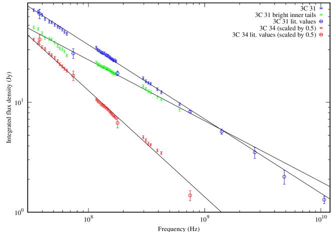
Figure 10: Spectrum of the integrated flux densities of 3C 31 and 34, where solid data points are our measurements and open data points are literature data. Lines show power-law fits to the data. The flux densities of 3C 34 were scaled by a factor of $0.5$ for clarity. The green data points show the flux densities of the bright inner tails of 3C 31 (see text for details).

In this appendix, we present some more detail about the observations (see Table 1 for a summary), in particular about the flux densities, source spectra and uncertainties. Table 3 contains the integrated flux densities of 3C 31, our science target, and of 3C 34, a compact, bright source located $0\aas@@fstack{\circ}9$ south-east of 3C 31. We used the CASA’s MS–MFS CLEANed LOFAR maps for 3C 31 and the AWIMAGER CLEANed LOFAR maps for 3C 34. AWIMAGER was used for 3C 34, because it allows for a correction for the LOFAR primary beam attenuation. The flux densities presented in this paper are scaled to the flux scale of Roger, Costain & Bridle (1973, hereafter RCB). Our own observations (LOFAR, VLA) were calibrated according to the calibrator models by Scaife & Heald (2012), which utilize the RCB scale. The 178-MHz values presented by Laing & Peacock (1980) were measured by Kellermann, Pauliny-Toth & Williams (1969, hereafter KPW) and scaled with a factor of $1.09$ to the RCB scale. Similarly, the 38-MHz value presented by Laing & Peacock (1980) was measured by KPW and scaled with a factor of $1.10$ to the RCB scale. The 74-MHz values were obtained from the VLSS redux survey, which are scaled to the calibrator models of Scaife & Heald (2012). The 750-MHz values are from Pauliny-Toth et al. (1966) and were scaled by a factor of $1.046$ in Laing & Peacock (1980). The remaining values were scaled from the flux scale of Baars, Genzel, Pauliny-Toth & Witzel (1977, hereafter B77) to the RCB scale using the factors from B77.

In order to check our flux scale, we investigated the spectrum of 3C 34 and compared it with values from the literature. This source is particularly well suited to a flux scale comparison since it is unresolved in our observations at 1 arcmin resolution, and similarly this is the case for the archive observations of the VLSS survey, WENSS survey and other archive data, which all have resolutions around 1 arcmin. In Fig. 10, we present our measured radio continuum fluxes of 3C 34 between 34 and 424 MHz obtained from our low-resolution maps. They can be well described by a power law with a radio spectral index of $-0.97\pm 0.01$ and with a reduced $\chi^{2}$ of $2.1$. For the error bars, we assumed a flux scale uncertainty of 3 per cent, which comes solely from the uncertainty on the flux calibrator 3C 48 (Scaife & Heald, 2012). We find that the power-law fit to our data agrees reasonably well with the literature values (shown as non-filled circles in Fig. 10).

For 3C 31, the comparison with literature values is more complex: the reason is that the source has faint and very extended radio tails, where the detection of emission is a function of sensitivity. The spectrum of the integrated emission (inner part plus tails) in Fig. 10 can be described by a power law, with a radio spectral index of $-0.67\pm 0.01$ between 34 and $10700$ MHz. The literature data points at 74 and 178 MHz are too low, which deserves some further investigation. The 178-MHz data point is based on the KPW measurements using the Cambridge pencil-beam interferometer (called 4CT pencil-beam by Laing et al., 1983) which had a FWHM of 20 arcmin in north-south orientation at the declination of 3C 31. As we shall see below, 3C 31 is essentially a source of 51 arcmin extending in north-south direction at this frequency, so the KPW 178-MHz observations will certainly have resolved the source, but will have detected the bright tails as a point-like source, picking up most of the flux. Similarly, the 74-MHz map of the VLSS redux survey (Lane et al., 2012) shows only the bright inner tails with little emission from the tails. We can check the consistency of our data points by simulating this effect, where we measured the flux density only in an area surrounding the bright inner tails (a rectangular box within R.A. $01^{\rm h}07^{\rm m}42^{\rm s}$–$01^{\rm h}07^{\rm m}00^{\rm s}$, Dec. $+32\degr 18\arcmin$–$32\degr 33\arcmin$). These data are plotted in Fig. 10 as triangles; they can be fitted by a power law with a radio spectral index of $-0.55\pm 0.01$ with reduced $\chi^{2}=2.2$ (the relatively high $\chi^{2}$ is due to the fact that the LBA in-band spectral index is too steep). Now the best-fitting power law is in very good agreement with the KPW data point. In the above measurements, we have assumed that the absolute calibration uncertainty is 3 per cent, which is the uncertainty of the calibrator model of Scaife & Heald (2012). This uncertainty is small, but is corroborated by our finding of a reduced $\chi^{2}=1.0$ when fitting the integrated 3C 31 flux densities (excluding the 74 and 178-MHz values) with a power law.

Finally, we discuss the uncertainties of our spatially resolved flux density measurements. In the following analysis, we use our low-resolution maps, where we average in a certain area (typically 3–10 beam areas) in order to find the averaged intensity. There are three sources of uncertainty which we take into account. Firstly, the calibration uncertainty $\rm cal_{e}=0.05$, which we assume to be 5 per cent. It is slightly larger than the uncertainty of the calibrator model, owing to the fact that imaging of extended emission results into an increased uncertainty due to the imperfect $(u,v)$-coverage. Secondly, there is the thermal noise in the $(u,v)$ visibilities, which results in approximately Gaussian fluctuations of the intensities in the map quantified by $\sigma_{I}$. Thirdly, we find that the average in the map is not always zero as expected for an interferometer. In areas of $\approx$100 beam areas, the average intensity should be within $0.1\sigma_{\rm rms}$ with zero. But in our maps this is not the case, the average intensity $\sigma_{\rm zero}$ is typically comparable to $|\sigma_{\rm rms}|$ (so it can be either positive or negative). We add the contributions in quadrature, so that we obtain for the error of the averaged intensities:

$$\sigma=\sqrt{({\rm cal_{e}}\cdot I_{\nu})^{2}+(\sigma_{I}/\sqrt{N_{\rm beam}})^{2}+(\sigma_{\rm zero})^{2}},$$ (15)

where $N_{\rm beam}$ is the number of beam areas within the integration area. In Table 4, we present the noise properties of our maps.

Table 4: Noise properties of our low-resolution maps (in units of $\rm mJy\,beam^{-1}$).

Map (MHz)	LBA (52)	HBA (145)	VLA (360)	WSRT (609)
$\sigma_{I}$	10	$1.5$	$1.0$	$0.8$
$\sigma_{\rm zero}$	3	$0.8$	$0.5$	$0.4$

Appendix B Adiabatic losses

The adiabatic losses (gains) are calculated as:

$$-\left(\frac{{\rm d}E}{{\rm d}t}\right)_{\rm ad}=\frac{1}{3}(\nabla\varv)\cdot E=\frac{E}{t_{\rm ad}}.$$ (16)

In cylindrical coordinates:

$$\nabla\varv=\frac{1}{\rho}\frac{\partial\varv_{\rho}}{\partial\rho}+\frac{\partial\varv_{z}}{\partial z}.$$ (17)

In the following, we assume that the tail expands (or contract) in a homologous way, so that:

$$\varv_{\rho}=\varv_{\rho 0}\cdot\frac{\rho}{r}\quad{\rm with}\quad\varv_{\rho 0}=\frac{\partial r}{\partial t}=\frac{\partial r}{\partial z}\cdot\varv_{z},$$ (18)

where $r$ is the tail radius. Hence:

$$\nabla\varv=2\frac{\partial r}{\partial z}\cdot\frac{\varv_{z}}{r}+\frac{\partial\varv_{z}}{\partial z}.$$ (19)

The adiabatic loss (gain) time-scale is then:

$$\frac{1}{t_{\rm ad}}=\frac{1}{t_{{\rm ad},r}}+\frac{1}{t_{{\rm ad},\varv}},$$ (20)

with the adiabatic losses (gains) through the tail lateral expansion (contraction):

$$t_{\rm ad,r}=\frac{2}{3}\frac{\partial r}{\partial z}\cdot\frac{\varv_{z}}{\partial z},$$ (21)

and the adiabatic losses (gains) though the tail’s velocity acceleration (deceleration):

$$t_{{\rm ad},\varv}=\frac{1}{3}\frac{\partial\varv_{z}}{\partial z}.$$ (22)

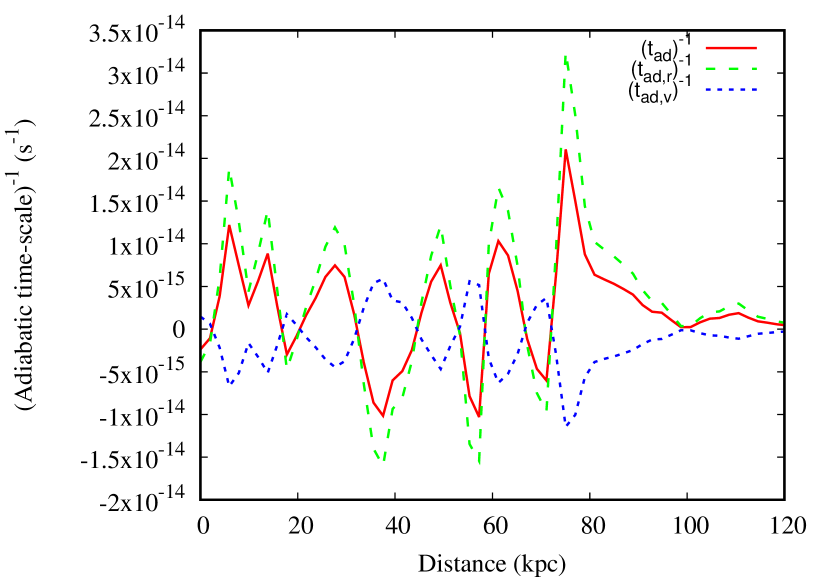
Figure 11: Inverse adiabatic time-scales in the northern tail with a decelerating flow ($\beta=-0.75$).

If the flow in the tail decelerates, the longitudinal compression cause adiabatic gains which offset partially the adiabatic losses due to the lateral expansion. For a flow velocity $\varv\propto r^{\beta}$, with $\beta=-2$ the adiabatic losses vanish. For $\beta=-0.75$, the adiabatic losses are significantly reduced as shown in Fig. 11.

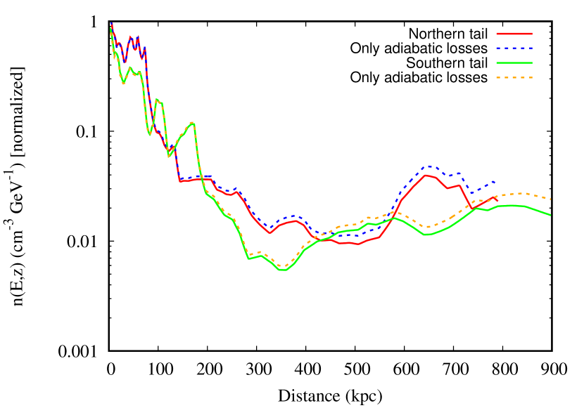
Figure 12: Comparison of the CRE (volume) number density at the critical frequency of 145 MHz with adiabatic models.

In order to test our numerical implementation, we compared our resulting CRE number density with the analytical expression (e.g. Baum et al., 1997):

$$n\propto(\varv\cdot A)^{-(\delta_{\rm inj}+2)/3}.$$ (23)

As can be seen in Fig. 12, the analytical expression is in close agreement with our numerical results. The small difference can be explained that in our model the CREs have additional spectral losses via synchrotron and IC radiation.

References

- Andernach et al. (1992) Andernach H., Feretti L., Giovannini G., Klein U., Rossetti E., Schnaubelt J., 1992, A&AS, 93, 331
- Arp (1966) Arp H., 1966, ApJS, 14, 1
- Baars et al. (1977) Baars J. W. M., Genzel R., Pauliny-Toth I. I. K., Witzel A., 1977, A&A, 61, 99
- Baum et al. (1997) Baum S. A., et al., 1997, ApJ, 483, 178
- Becker et al. (1991) Becker R. H., White R. L., Edwards A. L., 1991, ApJS, 75, 1
- Bicknell (1994) Bicknell G. V., 1994, ApJ, 422, 542
- Burbidge (1956) Burbidge G. R., 1956, ApJ, 124, 416
- Burch (1977) Burch S. F., 1977, MNRAS, 181, 599
- Burch (1979) Burch S. F., 1979, MNRAS, 187, 187
- Croston & Hardcastle (2014) Croston J. H., Hardcastle M. J., 2014, MNRAS, 438, 3310
- Croston et al. (2003) Croston J. H., Hardcastle M. J., Birkinshaw M., Worrall D. M., 2003, MNRAS, 346, 1041
- Eilek et al. (1997) Eilek J. A., Melrose D. B., Walker M. A., 1997, ApJ, 483, 282
- Ekers et al. (1981) Ekers R. D., Fanti R., Lari C., Parma P., 1981, A&A, 101, 194
- Fanaroff & Riley (1974) Fanaroff B. L., Riley J. M., 1974, MNRAS, 167, 31P
- Fomalont et al. (1980) Fomalont E. B., Bridle A. H., Willis A. G., Perley R. A., 1980, ApJ, 237, 418
- Hardcastle (2013) Hardcastle M. J., 2013, MNRAS, 433, 3364
- Hardcastle et al. (2002) Hardcastle M. J., Worrall D. M., Birkinshaw M., Laing R. A., Bridle A. H., 2002, MNRAS, 334, 182
- Hardcastle et al. (2016) Hardcastle M. J., et al., 2016, MNRAS, 462, 1910
- Harwood et al. (2013) Harwood J. J., Hardcastle M. J., Croston J. H., Goodger J. L., 2013, MNRAS, 435, 3353
- Heesen et al. (2014) Heesen V., Croston J. H., Harwood J. J., Hardcastle M. J., Hota A., 2014, MNRAS, 439, 1364
- Heesen et al. (2016) Heesen V., Dettmar R.-J., Krause M., Beck R., Stein Y., 2016, MNRAS, 458, 332
- Hughes (1991) Hughes P. A., 1991, Beams and Jets in Astrophysics. Cambridge University Press, Cambridge, UK
- Jaffe & Perola (1973) Jaffe W. J., Perola G. C., 1973, A&A, 26, 423
- Kellermann et al. (1969) Kellermann K. I., Pauliny-Toth I. I. K., Williams P. J. S., 1969, ApJ, 157, 1
- Kettenis et al. (2006) Kettenis M., van Langevelde H. J., Reynolds C., Cotton B., 2006, in Gabriel C., Arviset C., Ponz D., Enrique S., eds, ASP Conf. Ser. Vol. 351, Astronomical Data Analysis Software and Systems XV. p. 497
- Komossa & Böhringer (1999) Komossa S., Böhringer H., 1999, A&A, 344, 755
- Kuehr et al. (1981) Kuehr H., Witzel A., Pauliny-Toth I. I. K., Nauber U., 1981, A&AS, 45, 367
- Laing & Bridle (2002a) Laing R. A., Bridle A. H., 2002a, MNRAS, 336, 328
- Laing & Bridle (2002b) Laing R. A., Bridle A. H., 2002b, MNRAS, 336, 1161
- Laing & Bridle (2004) Laing R. A., Bridle A. H., 2004, MNRAS, 348, 1459
- Laing & Bridle (2014) Laing R. A., Bridle A. H., 2014, MNRAS, 437, 3405
- Laing & Peacock (1980) Laing R. A., Peacock J. A., 1980, MNRAS, 190, 903
- Laing et al. (1983) Laing R. A., Riley J. M., Longair M. S., 1983, MNRAS, 204, 151
- Laing et al. (2008) Laing R. A., Bridle A. H., Parma P., Feretti L., Giovannini G., Murgia M., Perley R. A., 2008, MNRAS, 386, 657
- Lane et al. (2012) Lane W. M., Cotton W. D., Helmboldt J. F., Kassim N. E., 2012, Radio Science, 47, RS0K04
- Lanz et al. (2011) Lanz L., Bliss A., Kraft R. P., Birkinshaw M., Lal D. V., Forman W. R., Jones C., Worrall D. M., 2011, ApJ, 731, 52
- Lara et al. (1997) Lara L., Cotton W. D., Feretti L., Giovannini G., Venturi T., Marcaide J. M., 1997, ApJ, 474, 179
- Ledlow et al. (1996) Ledlow M. J., Loken C., Burns J. O., Hill J. M., White R. A., 1996, AJ, 112, 388
- Longair (2011) Longair M. S., 2011, High Energy Astrophysics. Cambridge University Press, Cambridge, UK
- Martel et al. (1999) Martel A. R., et al., 1999, ApJS, 122, 81
- McMullin et al. (2007) McMullin J. P., Waters B., Schiebel D., Young W., Golap K., 2007, ASP Conf. Ser., 376, 127
- Mohan & Rafferty (2015) Mohan N., Rafferty D., 2015, PyBDSM: Python Blob Detection and Source Measurement, Astrophysics Source Code Library (ascl:1502.007)
- Morganti et al. (1988) Morganti R., Fanti R., Gioia I. M., Harris D. E., Parma P., de Ruiter H., 1988, A&A, 189, 11
- Offringa et al. (2010) Offringa A. R., de Bruyn A. G., Biehl M., Zaroubi S., Bernardi G., Pandey V. N., 2010, MNRAS, 405, 155
- Pandey et al. (2009) Pandey V. N., van Zwieten J. E., de Bruyn A. G., Nijboer R., 2009, in Saikia D. J., Green D. A., Gupta Y., Venturi T., eds, ASP Conf. Ser. Vol. 407, The Low-Frequency Radio Universe. p. 384
- Parma et al. (1999) Parma P., Murgia M., Morganti R., Capetti A., de Ruiter H. R., Fanti R., 1999, A&A, 344, 7
- Pauliny-Toth et al. (1966) Pauliny-Toth I. I. K., Wade C. M., Heeschen D. S., 1966, ApJS, 13, 65
- Perucho & Martí (2007) Perucho M., Martí J. M., 2007, MNRAS, 382, 526
- Perucho et al. (2014) Perucho M., Martí J. M., Laing R. A., Hardee P. E., 2014, MNRAS, 441, 1488
- Press et al. (1992) Press W. H., Teukolsky S. A., Vetterling W. T., Flannery B. P., 1992, Numerical recipes in FORTRAN. The Art of Scientific Computing. Cambridge University Press, Cambridge, UK
- Rau & Cornwell (2011) Rau U., Cornwell T. J., 2011, A&A, 532, A71
- Rengelink et al. (1997) Rengelink R. B., Tang Y., de Bruyn A. G., Miley G. K., Bremer M. N., Roettgering H. J. A., Bremer M. A. R., 1997, A&AS, 124, 259
- Roger et al. (1973) Roger R. S., Costain C. H., Bridle A. H., 1973, AJ, 78, 1030
- Rohlfs & Wilson (2004) Rohlfs K., Wilson T. L., 2004, Tools of Radio Astronomy. Springer, Berlin, Germany
- Scaife & Heald (2012) Scaife A. M. M., Heald G. H., 2012, MNRAS, 423, L30
- Scheers (2011) Scheers L. H. A., 2011, PhD thesis, Univ. Amsterdam
- Shimwell et al. (2017) Shimwell T. W., et al., 2017, A&A, 598, A104
- Strom et al. (1983) Strom R. G., Fanti R., Parma P., Ekers R. D., 1983, A&A, 122, 305
- Swarup (1991) Swarup G., 1991, in Cornwell T. J., Perley R. A., eds, ASP Conf. Ser. Vol. 19, in Radio Interferometry. Theory, Techniques, and Applications, eds. T.J. Cornwell, & R.A. Perley, IAU Colloq. 131, ASP Conf. Ser., 19, 376. pp 376–380
- Tasse et al. (2013) Tasse C., van der Tol S., van Zwieten J., van Diepen G., Bhatnagar S., 2013, A&A, 553, A105
- Weżgowiec et al. (2016) Weżgowiec M., Jamrozy M., Mack K.-H., 2016, Acta Astron., 66, 85
- Williams et al. (2016) Williams W. L., et al., 2016, MNRAS, 460, 2385
- Wright et al. (2010) Wright E. L., et al., 2010, AJ, 140, 1868
- Wykes et al. (2013) Wykes S., et al., 2013, A&A, 558, A19
- de Gasperin et al. (2012) de Gasperin F., et al., 2012, A&A, 547, A56
- van Breugel & Jagers (1982) van Breugel W., Jagers W., 1982, A&AS, 49, 529
- van Haarlem et al. (2013) van Haarlem M. P., et al., 2013, A&A, 556, A2
- van Weeren et al. (2016) van Weeren R. J., et al., 2016, ApJS, 223, 2
- van der Tol et al. (2007) van der Tol S., Jeffs B. D., van der Veen A.-J., 2007, IEEE Transactions on Signal Processing, 55, 4497