Pushing Memory Bandwidth Limitations Through Efficient Implementations of Block-Krylov Space Solvers on GPUs

Abstract

The cost of the iterative solution of a sparse matrix-vector system against multiple vectors is a common challenge within scientific computing. A tremendous number of algorithmic advances, such as eigenvector deflation and domain-specific multi-grid algorithms, have been ubiquitously beneficial in reducing this cost. However, they do not address the intrinsic memory-bandwidth constraints of the matrix-vector operation dominating iterative solvers. Batching this operation for multiple vectors and exploiting cache and register blocking can yield a super-linear speed up. Block-Krylov solvers can naturally take advantage of such batched matrix-vector operations, further reducing the iterations to solution by sharing the Krylov space between solves. Practical implementations typically suffer from the quadratic scaling in the number of vector-vector operations. We present an implementation of the block Conjugate Gradient algorithm on NVIDIA GPUs which reduces the memory-bandwidth complexity of vector-vector operations from quadratic to linear. As a representative case, we consider the domain of lattice quantum chromodynamics and present results for one of the fermion discretizations. Using the QUDA library as a framework, we demonstrate a 5$\times$ speedup compared to highly-optimized independent Krylov solves on NVIDIA’s SaturnV cluster.

1 Introduction

Two trends in HPC architectures present particular challenges to scientific software. The wider and wider architectures, in particular GPUs and Intel Xeon Phi processors, require an increasing amount of parallelism that cannot always be extracted from algorithms that had been considered state-of-the-art only a few years ago. Furthermore, the available memory bandwidth presents itself as the limiting factor in most scientific calculations. Hence, in addition to extracting parallelism exploiting data locality is key to achieve high performance. This has triggered a lot of algorithmic research, and the revisiting of older ideas can provide algorithmic speedup and high efficiency on current architectures even if these ideas had been discarded as less efficient decades ago.

An important example of an older idea, and the one of focus in this work, is the block-Krylov solver method. This method reduces the iteration count by processing blocks of right hand sides (rhs) simultaneously, augmenting the Krylov space of each rhs by information from the other rhs in the block. On its own, this idea naturally generates more parallelism and exploits data-locality with the simultaneous application of a matrix-vector operator per algorithm iteration.

As will be discussed in more depth later, the original formulation of block-Krylov methods suffered from numerical instabilities [1] due to overlapping Krylov subspaces and a quadratic scaling in the number of BLAS-like operators with the number of rhs. Later algorithmic developments efficiently overcame the issue of numerical instabilities [2], but the issue of quadratic scaling in operations still rendered the method largely unfeasable.

In the modern era, this quadratic scaling of operations in a problem featuring a large amount of spatial locality becomes a benefit. Block-Krylov methods naturally provide the arithmetic intensity required to offset memory bandwidth constraints. An efficient implementation offers a significant speedup on top of the multiplicative speedup offered by the features of the algorithm alone. Such algorithms are very suitable for current and future HPC systems, and will continue to contribute meaningful speedup and develop increased prominence as we trend towards the exascale and beyond.

GPUs provide the perfect setting for demonstrating the block-solver algorithm, and as such will be the architecture of choice for the study performed here. Present GPUs typically feature thousands of floating point units coupled to a very wide and fast memory bus, and, as common to many-core processors, a high algorithmic arithmetic intensity is required to reach a reasonable percentage of peak performance. In this work we utilize the QUDA library [3] to implement a high-efficiency block CG solver that is able to exploit the growing imbalance between floating-point peak performance and memory bandwidth.

QUDA is a domain-specific library which targets lattice quantum chromodynamics (LQCD), the numerical simulations of the theory of the strong force that underpins nuclear and particle physics. In the past few years, LQCD applications have been continually under intensive development to address computationally demanding scientific problems in nuclear and high energy physics. These algorithmic improvements and the advances in computing architectures now allow predictions with errors comparable or even below experimental results obtained at large particle colliders like the LHC at CERN. To control the statistical error, a typical computational scenario requires the solution of many systems of linear equations with the same matrix but different rhs. The development of efficient implementations of block-Krylov methods serves as an immediate win in the LQCD community.

We emphasize that our target problems within LQCD are a representative case of an algorithmic problem present across the discipline of scientific computing. We will not attempt an exhaustive list of fields where the iterative solution of a sparse matrix-vector system against multiple rhs is a predominant use of computer cycles. As a subset of examples, though, we point the interested reader to literature concerning the simulation of quasistatic electromagnetic fields [4], electromagnetic 3D modeling [5], scattering and radiation [6], and fluid simulations [7, 8], including aircraft modeling and weather forecasts. Again, each of these fields can benefit from the efficient implementation of a block-Krylov method described here.

As a last note of importance, the developments in this work are in large part orthogonal and complimentary to existing approaches to reduce the time-to-solution of the problem of solving multi-rhs systems. Block-Krylov methods are compatible with deflation methods, where low eigenvectors of the linear system are computed and projected out which provides an acceleration in its own right (see, for example, [9, 10]). Block methods are also relevant for components within adaptive multigrid [11, 12] and the related inexact deflation [13], which are mathematically optimal (no condition number dependence and constant iteration count with volume). That being said, we will not discuss these complimentary approaches further.

Our implementation of a block CG solver is, to the best of our knowledge, the first efficient implementation of a reliable block solver at scale on GPUs. Previous implementations either ran on CPU [14, 15] or didn’t provide scaling results [16, 17, 18]. We take advantage of mixed precision to mitigate memory-bandwidth limitations and – as a novel development – implement a first generalization of the idea of reliable updates [19] to block solvers, a necessary step to correct for round-off errors due to the use of mixed precision. We employ block BLAS operations to saturate memory bandwidth and exploit data locality for both streaming and reduction BLAS operations, allowing us to take advantage of the extra compute power offered by modern nodes. Last, we achieve good strong scaling both by an improved implementation of a multi-right-hand-side-stencil operation and by a new interface which allows us to overlap communications inherent to stencil operations with independent computation.

This paper is organized as follows: in $\S$2 we highlight previous work in this area, in $\S$3 we give an overview of the LQCD computations, and we give an overview of the block CG solver in $\S$4. We introduce the QUDA library in $\S$5 and describe in the detail the optimization techniques employed in our block CG implementation in $\S$6. We show weak scaling performance curves from one and two NVIDIA Quadro GP100 GPUs, and more significantly, strong-scaling performance curves from the NVIDIA SaturnV DGX-1 supercomputer in $\S$7; we discuss future implications in $\S$8 before finally concluding with $\S$9.

2 Previous Work

The first use of GPUs for LQCD was reported more than a decade ago [20], before the advent of compute APIs, necessitating the use of graphics APIs. Since then LQCD has been at the forefront of the adoption of GPUs in HPC. Notable publications include multi-GPU parallelization [21, 22, 23], the use of additive-Schwarz preconditioning to improve strong scaling [24], implementation of multi-grid solvers [25], software-managed cache-blocking strategies [26], and JIT-compilation to enable the offload of the entire underlying data-parallel framework of the Chroma [27] application without any high-level source changes [28].

Block-Krylov-space methods go back to the 1980s [29] for CG and Bi-CG solvers. By solving multiple rhs in parallel they combine the benefit of increased parallelism and data locality with an reduced iteration count compared to a non-block method. The naïve implementation was found to suffer from stability issues and the subsequent revisions which introduce explicit re-orthogonalization [2] have significantly improved their general usability. However, the stability improvements come at the cost of implementation efficiency and can become prohibitively expensive outweighing any benefit over non-block solvers. In LQCD, block methods have not seen wide adoption. The use of block BiCGSTAB has been reported in [30, 31, 32]. Birk and Frommer generalized block methods also for the use in shifted systems [33, 34], which dominate the runtime in Monte Carlo ensemble generation in LQCD.

To our best knowledge block-Krylov methods have not been reported to be efficiently implemented for LQCD on GPUs. The benefit of using the block idea for the matrix-vector operation to multiple rhs has been reported on GPU and Intel Xeon Phi [35, 36], however there it was combined with a regular CG solver resulting in only a pseudo-block algorithm.

3 Lattice Quantum Chromodynamics

3.1 Computational Method and Theoretical Relevance

LQCD calculations are typically Monte-Carlo evaluations of Euclidean-time path integrals. A sequence of configurations of the gauge fields $U$ is generated in a process known as configuration generation. The gauge configurations are importance-sampled with respect to the lattice action and represent a snapshot of the QCD vacuum. Once the field configurations have been generated, one moves on to the second stage of the calculation, known as analysis. In this phase, observables of interest are evaluated on the gauge configurations in the ensemble, and the results are then averaged appropriately, to form ensemble averaged quantities. The analysis phase can be task parallelized over the available configurations in an ensemble and is thus extremely suitable for capacity-level work on clusters, though calculations on the largest ensembles can also make highly effective use of capability-sized partitions of leadership supercomputers. These calculations rely heavily on computational resources, with LQCD workloads accounting for a significant fraction of supercomputing cycles consumed worldwide.

The numerical calculation we will focus on in this study is that of the fermion magnetic moment. Abscent the contributions from QCD, this quantity can be computed within the standard model to high accuracy. The Dirac equation predicts ${\bf\mu}=ge/(2m){\bf S}$, where ${\bf\mu}$ is the magnetic moment, $e$ is the fermion electric charge, $m$ is its mass, ${\bf S}$ is the spin and $g$ is the Landé $g$-factor. For free fermions $g=2$, but when we introduce electro-weak and strong force (QCD) interactions, $g$ receives perturbative and non-perturbative corrections, which are gathered in the anomalous magnetic moment, defined as $a_{\mu}=\frac{g-2}{2}$, which measures how far we are from the free fermion case. The particular case of the muon is extremely interesting, because there is a $3\sigma$ difference between the theoretical and experimental determinations of $a_{\mu}$. It is of the utmost importance to improve the precision of both determinations, for this difference can be an indicative of new fundamental physics. The largest part of the error in the theoretical determination of $a_{\mu}$ comes from non-perturbative QCD contributions, thus the relevance of our target numerical calculation. The LQCD calculation of this contribution is essentially computing the trace of the inverse of a large sparse matrix, the exact calculation of which is unfeasible. Therefore the calculation relies on stochastic estimators [37], involving solving thousands of rhs per linear system for many different linear systems. At present, the cost of solving a requisite number of linear systems accounts for $\sim 90\%$ of the total computational time.

3.2 Dirac PDE Discretization

The fundamental interactions of QCD are encoded in the quark-gluon interaction differential operator known as the Dirac operator. As is common in PDE solvers, the derivatives are replaced by finite differences. Thus on the lattice, the Dirac operator becomes a large sparse matrix, $M$, and the calculation of quark physics is essentially reduced to many solutions to systems of linear equations given by

$$Mx=b.$$ (1)

A small handful of discretizations are in common use, differing in their theoretical properties. Here we focus on the so-called staggered form [38], which is a central-difference discretization; where the infamous fermion doublers (which arise due to the instability in the central difference approximation) are removed through “staggering” the underlying fermionic (spin) degrees of freedom onto neighboring lattice sites. This essentially reduces the number of spin degrees of freedom per site from four to one, which reduces the computational burden significantly. This transformation, however, comes at the expense of increased discretization errors, and breaks the so-called quark-flavor symmetry. To reduce these discretization errors, the gauge field that connects nearest-neighboring sites on the lattice is smeared, which essentially is a local averaging of the field. There are many prescriptions for this averaging; and here we employ the popular HISQ procedure [39]. When acting in a vector space that is the tensor product of a four-dimensional discretized Euclidean spacetime (the lattice) and color space, the HISQ stencil operator is given by

$$M_{x,x^{\prime}} =-\frac{1}{2}\displaystyle\sum_{\mu=1}^{4}\bigl{(}\hat{U}_{x}^{\mu}\,\delta_{x+\hat{\mu},x^{\prime}}\,+\hat{U}_{x-\hat{\mu}}^{\mu\dagger}\,\delta_{x-\hat{\mu},x^{\prime}}+$$

$$\quad\quad\quad\quad\check{U}_{x}^{\mu}\,\delta_{x+3\hat{\mu},x^{\prime}}\,+\check{U}_{x-3\hat{\mu}}^{\mu\dagger}\,\delta_{x-3\hat{\mu},x^{\prime}}\bigr{)}+m\delta_{x,x^{\prime}}$$ (2)

Here $\delta_{x,y}$ is the Kronecker delta; $\hat{U}$ ($\check{U}$) is the “fat” (“long”) matrix field that connects lattice sites that are one hop (three hops) apart. These are fields of $3\times 3$ matrices acting in color space that live between the spacetime sites (and hence are referred to as link matrices); and $m$ is the quark mass parameter. The indices $x$ and $x^{\prime}$ are spacetime indices (the color indices have been suppressed for brevity). This matrix acts on a vector consisting of a complex-valued three-component color-vector for each point in spacetime. When represented as a sparse matrix, there are 16 off-diagonal matrices, representing the 1-hop and 3-hop link matrices. Given the stencil coefficients are dependent on the underlying gauge field, the coefficients vary for each configuration in the Monte Carlo ensemble.

For the current problem sizes of interest, the linear system has a rank that ranges from $V\approx 10^{6}$ for a small lattice volume ($32^{4}$) up to $V\approx 10^{10}$ for the largest ($144^{3}\times 288$). Furthermore, $M$ is typically very ill conditioned: the highest eigenvalue is of order $O(1)$, but the lowest one is determined by the quark mass, which introduces a lower bound in the spectrum. The most physically interesting cases involve very light or massless quarks, and in that case the lower bound can become as low as $O(1/V)$. The standard workhorse algorithm employed is the CG algorithm, where the normal operator $A=M^{\dagger}M$ is used since $M$ itself is not Hermitian. In our case we work with the Schur decomposed version of $M$, which is smaller in size and better conditioned than $M$ or $A$, although it still shares the problems of the original linear system.

4 Block CG Solver

The block-CG algorithm was first published in [29]. The idea is to apply the CG solver [40] to a block of $N$ rhs. In a broad sense, scalars in the CG algorithm become $N\times N$ matrices and for $N=1$ the algorithm reduces to the regular CG.

In infinite precision the block-CG algorithm will converge in at most $L/N$ iterations where $L$ denotes the length of the vectors, or the rank of the matrix $M$. While the algorithm maintains a simple link to regular CG, it has issues with numerical stability and will break down if the residual matrix $\left(R^{\dagger}R\right)$ becomes singular, i.e. if the Krylov subspaces of the different vectors in the block overlap. There have been various attempts to remedy this, including dynamically monitoring the rank and removing any linearly dependent columns [1]. A more suitable approach was introduced in [2], where a set of retooled block-CG methods are discussed. The common idea is to use a QR decomposition to enforce the full rank of the $P$ and $R$ matrices and thus avoid any rank deficits and the need to dynamically remove columns from the algorithm. We will only discuss the blockCGrQ variant, which applies the factorization to $R$, as shown in algorithm 1. This variant has been shown to generally behave the best in terms of stability and performance [2].

Algorithm 1 blockCGrQ: Solve $A^{L\times L}X^{L\times N}=B^{L\times N}$

1:$A\in\mathcal{C}^{L\times L}$; $R,B,X,Q\in\mathcal{C}^{L\times N}$; $C,S,\beta\in\mathcal{C}^{N\times N}$

2:procedure blockCGrQ($X^{L\times N},B^{L\times N}$)

3:     $R=B-AX$

4:     $QC=R$ $\triangleright$ QR decomp.

5:     $S=\mathbb{I}^{N\times N}$

6:     $P=0$

7:     while not converged do

8:         $P=Q+PS^{\dagger}$

9:         $\beta=\left(P^{\dagger}AP\right)^{-1}$

10:         $X=X+P\beta C$

11:         $QS=Q-AP\beta$ $\triangleright$ QR decomp.

12:         $C=SC$

13:     end while

14:end procedure

An important observation is that any block algorithm will naively show quadratic scaling in the number of BLAS vector-vector operations and reductions. E.g., the BLAS-1 operations from CG become BLAS-3 operations. Moreover, the factorization required for stability increases the cost per iteration. We will address these concerns when we discuss our implementation in §6.

5 The QUDA Library

QUDA (QCD on CUDA) is a library that aims to accelerate LQCD computations through offload of the most time-consuming components of an LQCD application to NVIDIA GPUs. It is a package of optimized CUDA C++ kernels and wrapper code, providing a variety of optimized linear solvers, as well as other performance critical routines required for LQCD calculations. All algorithms can be run distributed on a cluster of GPUs, using MPI to facilitate inter-GPU communication. On systems with multiple GPUs that are directly connected with either NVLink or PCIe, QUDA will take full advantage utilizing direct DMA copies between GPUs to minimize the communication overhead. Similarly, on systems that support GPU Direct RDMA, where the NIC can read/write directly to the GPU’s memory space, QUDA will utilize this to improve multi-node scaling. It has been designed to be easy to interface to existing code bases, and in this work we exploit this interface to use the popular LQCD application MILC [41] as a driver. The QUDA library has attracted a diverse developer community and is being used in production at U.S. national laboratories, as well as in locations in Europe and India. The latest development version is always available in a publicly-accessible source code repository [42].

The general strategy is to assign a single GPU thread to each lattice site. Each thread is then responsible for all memory traffic and operations required to update that site on the lattice given the stencil operator. Since the computation always takes place on a regular grid, a matrix-free approach is used. Maximum memory bandwidth is obtained by reordering the vector and link fields to achieve memory coalescing, e.g., using structures of float2 or float4 arrays, and using the texture cache where appropriate. Memory-traffic reduction is employed where possible to overcome the relatively low arithmetic intensity of the Dirac matrix-vector operations, which would otherwise limit performance. The primary strategy employed here is the use of low-precision data storage, utilizing single precision or a custom 16-bit fixed-point storage format (hereon referred to as “half precision”) together with mixed-precision linear solvers to achieve high speed with no loss in accuracy [3].

The library has been designed to allow for maximum flexibility with respect to algorithm parameter space and maximum performance. For example, all lattice objects (fields) maintain their own precision and data ordering as a dynamic variable. This allows for run-time policy tuning of algorithms; these parameters are then bound at kernel launch time when the appropriate C++ template is instantiated corresponding to these parameters.

In fact the use of this autotuning is key to achieving high performance: all kernel launch parameters (block, grid, and shared memory size) are autotuned upon the first call and cached for subsequent reuse. In the work presented here, we extended the autotuner extensively as an algorithm-policy tuner, discussed in §6.2 and §6.4.

6 Efficient Implementation of BlockCGrQ

Our implementation of blockCGrQ integrates many developments to overcome the issues discussed in §1 and §4. We will address these as we step through algorithm 1 and discuss the details of our efficient implementation. We may expect a reduced time to solution from blockCGrQ due to the reduced iteration count. An additional benefit can be achieved by applying the matrix-vector operation to multiple rhs in parallel, exploiting data locality in this operation; see §6.2. This is countered, however, by the quadratic increase in the number of BLAS-1 vector-vector operations, which generalize to BLAS-3 matrix-matrix operations, as well as an additional cost due to the factorization employed on lines 4 and 11.

We make use of a thin QR factorization [45]. By strict mathematical definition, the QR factorization of a rectangular matrix would be given as $\tilde{Q}^{L\times L}\tilde{R}^{L\times N}=M^{L\times N}$, where $\tilde{Q}$ is dense with orthonormal columns and $\tilde{R}$ is upper right triangular. A dense matrix of dimension $L\times L$ is prohibitive in LQCD as $L$ is typically of $\mathcal{O}(10^{6-9})$. However, the matrix $\tilde{R}$, being upper right triangular, has zeros in the bottom $(L-N)\times N$ components. Thus, the right $(L-N)\times N$ columns of $\tilde{Q}$ are irrelevant and can be dropped. This leads to the thin QR factorization given in algorithm 2, which of note contains structured BLAS operations.

Algorithm 2 thin QR: Decompose $Q^{L\times N}R^{N\times N}=M^{L\times N}$

1:procedure thinQR($M^{L\times N}$)

2:     $H^{N\times N}=\left(M^{L\times N}\right)^{\dagger}M^{L\times N}$

3:     $\left(R^{N\times N}\right)^{\dagger}R^{N\times N}=H^{N\times N}$ $\triangleright$ Cholesky decomp.

4:     $Q^{L\times N}=M^{L\times N}\left(R^{N\times N}\right)^{-1}$

5:end procedure

With this exposition, we can now decompose the operations in our implementation of algorithm 1 into four classes: matrix-block-vector operations in lines 3 and 9; block-vector-block-vector streaming operations in lines 8 and 10; block-vector-block-vector reduction operations in lines 3 and 9; and small dense matrix operations. The latter three kinds of operations are also embedded in the thin QR decomposition.

A key ingredient for the implementation is generalizing our lattice fields from a single vector of length $L$ to an efficient data structure of size $L\times N$. We refer to these $L\times N$ matrices as composite fields with details discussed in §6.1. We will discuss how to exploit data locality to reuse $A$ in the matrix-vector operation to obtain a speedup per rhs in §6.2 and mitigate the naïve quadratic scaling of the block-vector-block-vector operations to achieve an overall multiplicative speedup in §6.3, 6.4.

For all small $N\times N$ matrices we exploit the Eigen library [46] for the Cholesky decomposition of $R$. Given that $N\leq 64$, these matrices are comparably small and all operations are negligible in the overall runtime.

Mixed-precision implementation

For our mixed-precision implementation we rely on “reliable updates”, referring to a class of residual correction methods described, e.g., in [19, 47]. A general residual correction method periodically updates the iterated residual with the true residual from the iterated solution. This corrects for numerical round-off effects and, by extension, possible instability in Krylov methods. In the case of mixed-precision solves, this correction is often essential to monitor convergence in a meaningful fashion. We based our implementation of reliable updates on the implementation given in [3], with important deviations presented in algorithm 3. We believe that this is the first implementation of a residual correction method to improve the convergence of a block-Krylov method.

Algorithm 3 Reliable updates

1:procedure ReliableUpdate($X^{L\times N},\widehat{Q}^{L\times N},S^{N\times N}$)

2:     $Y^{L\times N}=Y^{L\times N}+X^{L\times N}$ $\triangleright$ caxpy_5d

3:     $X^{L\times N}=0$

4:     $R^{L\times N}=B^{L\times N}-A^{L\times L}Y^{L\times N}$ $\triangleright$ Block Mat-Vec, caxpy_5d

5:     $\widehat{Q}^{L\times N}C^{L\times N}=R^{L\times N}$ $\triangleright$ thin QR

6:     $S^{N\times N}=C^{N\times N}\left(C_{old}^{N\times N}\right)^{-1}$

7:end procedure

Like in [3], we employ a persistent fine precision accumulator for the iterated solution, denoted by the block vector $Y^{L\times N}$. The block vector $X^{L\times N}$ only contains the iterated update to the solution between reliable updates, which, in contrast to [3], is maintained at full precision. The block vectors $P^{L\times N}$ and $Q^{L\times N}$ are maintained in lower precision. We perform a reliable update when the maximum relative iterated residual decreases by a factor of $\delta$. We use the relative residual as opposed to the absolute residual to perform a meaningful comparison between the different rhs vectors. The iterated residual can be computed after $C^{N\times N}$ is updated on line 12 of algorithm 1 by the identity $\left|R^{L\times N}_{i}\right|^{2}=\sum_{j}\left|C_{ij}^{N\times N}\right|^{2}$.

When a reliable update is triggered, the current iterated solution update $X^{L\times N}$ is accumulated into the full solution $Y^{L\times N}$ and the true residual is computed in full precision, as implemented in [3]. As required by blockCGrQ, we perform a thin QR factorization of the true residual. The update of $S^{N\times N}$ on line 6 of algorithm 3 forces the preservation of the identity given in equation (6.1) of [2]. The new $S^{N\times N}$ enters the update of $P^{N\times N}$ on line 8 of algorithm 1. This is essential to maintain one of the defining properties of blockCGrQ, $\left(Q^{L\times N}_{old}\right)^{\dagger}P^{L\times N}=\mathbb{I}^{N\times N}$, noted below figure 6.1 of [2], which is intimately connected to preserving the Krylov search space through the reliable update.

6.1 Composite Fields

In order to provide both ease of expressibility and high efficiency for the block-solver implementation, we extended QUDA to facilitate the application of the required linear algebra components on both sets of vector fields and individual vector fields. To this end we enhanced QUDA’s vector-field container ColorSpinorField, with a new attribute: whether it is a composite field or not. When it is a composite field, the container contains an STL vector of component ColorSpinorFields, whose memory refers to contiguous subsets of the parent composite. The composite field can thus be viewed as a single higher-dimensional object while providing accessor methods to expose individual components or the entire STL vector. This functionality of being able to switch between block and scalar methods while using the same data structure was critical in algorithm prototyping, debugging, and performance analysis.

6.2 Block-optimized Matrix-vector Product

The efficient application of the stencil operator, equation 2, is critical in a performance-optimized iterative linear solver. The stencil connects lattice sites that are one and three hops away in all dimensions in both positive and negative directions relative to the center site. To apply the stencil, we load the neighboring sites (6 numbers per site), the link matrix between the neighboring sites (18 numbers per matrix), perform the link-matrix times vector multiplication and accumulate to the new resulting center value. With 16 neighbors, this means each application of the operator requires 1158 flops and 390 words of memory traffic per lattice site, for an arithmetic intensity of 0.74 in single precision. The Pascal-generation GPUs used in this study can achieve a STREAM bandwidth of 575 GB/s, giving a naïve performance upper bound of 435 GFLOPS in single precision, compared to a peak of 10.1 TFLOPS, so we can see that any naïve implementation of the stencil would be memory-bandwidth bound.

In this specific algorithm, we apply this stencil to multiple vector fields simultaneously, and as such we have implemented a block-optimized stencil operator which allows us to severely reduce the contribution of link matrices to the overall memory traffic. In the usual single-rhs stencil operator, a volume of threads are launched, each assigned to a grid point. Threads are partitioned into a grid of thread blocks, where each thread block runs on a given streaming multiprocessor (SM), roughly equivalent to a CPU core. This provides enough thread-level parallelism to saturate the GPU memory bus.

When augmenting the GPU kernel to apply the stencil to multiple sites, we utilize the Cartesian thread indexing that GPUs expose: we map the y-thread dimension to the rhs index, keeping the x-dimension thread mapping to grid points unchanged. Since all threads in the same thread block share the same L1 cache, threads with a common grid index in the same thread block (e.g., different rhs index) are able to exploit temporal locality to share the link matrix load. The optimal x-y shape of the thread block is autotuned: this effectively optimizes for the competing localities (link-matrix element reuse versus vector-field neighbor reuse) and L1 vs L2 reuse (larger blocks will result in more L1 cache hits versus L2 cache hits).

In figure 1 we plot the performance results from the block-optimized stencil for a $24^{4}$ lattice. We use the colors red, green, and blue to represent double, single, and half precision, respectively. As an alternative classifier, the bottom, middle, and top batches of lines correspond to double, single, and half precision, prespectively. The solid lines with filled squares represent the performance of the cache-tiled implementation for double, single and half precision. While we see an improvement in performance with increasing rhs, the improvement for single precision, and in particular half precision is milder. Further analysis revealed the limiting factor to be load-instruction rate and cache bandwidth. To alleviate this we utilize a register-tiling approach where each thread is responsible for updating multiple rhs at constant grid index. The register-tile size is a template parameter in our code, with tile sizes $1\ldots 6$ instantiated. The final algorithm is a hybrid of cache and register tiling, where the optimal balance is found by the autotuner. The performance of the hybrid approach is shown in the dashed lines with filled diamonds, where we see minimal improvement for double performance, but significant improvement for both single and half precision. The erratic behavior at larger numbers of rhs is due to numbers of rhs that are not divisible by a tile size greater than 1 or 2. We also include a roofline extrapolation of the expected performance from exploiting the temporal locality of the link-matrix elements. Here we are also assuming perfect reuse of vector-field loads in the x dimension, and 50% in the y dimension (e.g., for every 16 grid points each thread loads, 6 of them are cached). For double and single precision, the hybrid tiling performance broadly matches the roofline expectation, given as the dotted line with filled triangles, with the roofline actually underestimating performance at small rhs in single precision: this is due to the cache-hit rate for the vector-field loads being greater than in the model. For half precision, even with hybrid tiling, the kernel remains load-instruction-rate bound, as evidenced by it failing to match the roofline performance model.

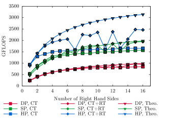
Figure 1: The performance in GFLOPS of the stencil operator as a function of number of rhs vectors. Measurements are taken from a $24^{4}$ lattice. The colors red, green, and blue correspond to double, single, and half precision, respectively. The solid lines with filled squares represent the cache-tiling implementation, the dashed lines with filled diamonds the cache-and-register-tiling implementation, and the dotted lines with filled triangles is a roofline model of the performance. Tests were performed on a Quadro GP100 GPU.

The multi-GPU parallelization of stencil operators in QUDA has been reported elsewhere [21, 24]. The essential strategy is to overlap the communication of the halo region with the computation on the interior, with a final halo update kernel required to produce the complete answer. The ability to hide the communication scales with the surface-to-volume ratio, hence strong scaling is often communication limited. To maximize performance we made use of two key technologies:

• Peer-to-peer communication: direct communication between GPUs within the same node

• GPU Direct RDMA: direct communication between the GPUs and the NICs maximizing the inter-node communication rate

On a sufficiently distributed system, the communication of the halo region can take much longer than the computation on the interior. To help mitigate this, we have implemented an interface to the stencil kernel, such that an algorithm can schedule additional computation during the halo exchange that is independent of the stencil application. This is an important optimization for a wide class of algorithms, but in particular for the block-Krylov method discussed here since the amount of work scales with the number of right hand sides.

We note that on line 10 of algorithm 1, the update of the iterated $X$ can be scheduled to occur at any point after the calculation of $\beta$. We thus move the update of $X$ to occur during the stencil application in the next iteration. This depends on maintaining the “old” version of $P$ from before the update on line 8. Our implementation of line 8 preserves the state of $P$ from when $X$ would normally be updated at no memory traffic overhead—there is no additional cost from updating $X$ during the stencil application. This allows for a simplified interface where the scheduled compute can still occur during the would-be communication on a single node at no additional cost. One exception to this situation is when a reliable update is triggered. In that case, $X$ must be updated immediately. This is infrequent and thus negligible.

6.3 Streaming Multi-BLAS

For the block linear algebra operations we distinguish between block-AXPY-type operations and block-DOT-type operations. They differ conceptually, and in implementation, since the latter require global reductions. We refer to the former as Streaming Multi-BLAS, which we focus on here, and the latter as Reduction Multi-BLAS, which we delay until §6.4.

For the discussion here we chose a caxpy operation as the representative example. In blockCGrQ it is used in the form $Y^{L\times N}=Y^{L\times N}+X^{L\times M}a^{M\times N}$, or at the element level,

$$y_{k,j}=y_{k,j}+\sum_{i=0}^{N-1}x_{k,i}a_{i,j}.$$ (3)

Note that in the case of blockCGrQ we only need the case $N=M$, and as such $a^{N\times N}$ is a square matrix. We will assume $M=N$, the number of right hand sides, unless noted otherwise.

Equation 3 can be implemented as separate caxpy applications for each component of $\alpha^{N\times N}$. This implementation incurs a quadratic scaling of memory traffic and floating-point operations with $N$. Due to the low arithmetic intensity, the operation is severely limited by memory bandwidth and becomes prohibitively expensive as the number of right hand sides increases. A block caxpy takes advantage of the memory reuse inherent in equation 3 by re-expressing the set of vector-vector operations as a single matrix-matrix computation. For a given component $k$, block caxpy loads all $N$ components of $X^{L\times N}_{k}$ and $Y^{L\times N}_{k}$, performs the $N^{2}$ multiplications and additions, then saves all $N$ components of $Y^{L\times N}_{k}$ back to memory. The quadratic scaling of memory traffic becomes a linear scaling. Since the required flops remains well below the theoretical peak of modern GPUs, the quadratic cost of the algorithm shifts to lower latency cache load instructions which can take advantage of the spatial locality inherent to cache.

We have developed a general framework to perform such BLAS-3-type operations. We distribute the update of a single block vector constituent $k$ over $N$ threads on the GPU by assigning a unique constituent $y_{k,j}$ to each thread. Each thread is tasked with updating $y_{k,j}$ with the contributions from each $x_{k,i}$. Similar to the block-matrix-vector product in $\S\ref{sec:dslash}$, we use CUDA thread blocks to ensure that for a given $k$, all $j=0,\ldots,N$ are scheduled to the same SM. This guarantees that all $x_{k,i}$ reside in L1 cache and can be shared between all $N$ threads, exploiting spatial locality.

We take extensive advantage of C++ templating which allows the compiler to perform additional optimizations. We template over all possible combinations of the block sizes of $N$ and $M$ up to a sufficient maximum, enabling the compiler to perform loop unrolling. In addition, we template over all possible precisions for $Y^{L\times M}$ and all equal or lower precisions for $X^{L\times N}$. This optimization is essential for efficient mixed-precision block-Krylov methods. Furthermore we take advantage of QUDA’s autotuner in the developed BLAS-3 framework. Finally, we note that while the block caxpy is essentially a CGEMM operation included with every standard BLAS library, the disparity between the sizes of $N$ and $L$ ($L\gg N$) are such that no out-of-the-box BLAS library would perform well for this use case, requiring us to implement our own framework to this end.

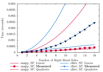
Figure 2: The average cost, in seconds, of applying a square block caxpy and a square block cDotProduct as a function of the number of right hand sides. Measurements are taken from a $24^{4}$ lattice, in single precision. Both are contrasted against a best-case linear and a worst-case quadratic extrapolation from a single caxpy and cDotProduct. The block caxpy features linear scaling for a wide range of $N$. In contrast, the block dot product shows quadratic scaling even for small $N$. Tests were performed on a Quadro GP100 GPU.

Figure 2 shows that the cost of the block-caxpy operation scales linearly for a wide range of the number of rhs. The eventual deviation from linear scaling is due to the less-penalizing cache traffic. This is consistent with figure 3, where we see that the performance of the block-capxy operations also scales linearly in $N$. Note that due to finite cache sizes there is a turnover point in $N$ where it is advantageous to recursively divide the block BLAS into tiles, e.g., to split a $24\times 24$ block operation into four $12\times 12$ block operations. We refer to a recursed segment of the BLAS operation as a “tile”, and its size as the “tile size”.

There are two places in algorithm 1, lines 4 and 8, where we can take advantage of recursively divided block-BLAS operations and perform additional optimizations. In each case, we take advantage of the triangular structure of the small, dense matrix $A$ and skip computing empty tiles. The benefit of this optimization scales quadratically in $N$ over tilesize. However, we observe that this optimization is only beneficial simultaneous with when tiling itself becomes beneficial.

6.4 Reduction Multi-BLAS

For the discussion of block reductions, we will consider the representative case of a complex dot product, or cDotProduct, $K^{N\times M}=\left(X^{L\times N}\right)^{\dagger}Y^{L\times M}$. At the component level it is defined as

$$k_{ij}=\sum_{k=0}^{L-1}x_{k,i}^{*}y_{k,j}.$$ (4)

In the following we again limit our discussion to the case $N=M$ and assume that the resulting matrix $K^{N\times N}$ is Hermitian, which is always true in blockCGrQ.

At a basic level, our software implementation of block reduction operations is similar to the implementation of Streaming Multi-BLAS operations. The goal is again to achieve an implementation of Reduction Multi-BLAS operations that obeys a linear scaling in memory traffic as opposed to a quadratic scaling. We template over both the left and right block vectors, allowing the compiler to generate efficient code for every combination of left and right block sizes and apply the autotuner separately to each combination. Each thread is responsible for the multiplication of a single component $y_{k,j}$ with every component of $x_{k,i}$. We utilize the CUB library [48] for an efficient thread block and inter-block reduction per site. We still recursively divide block reduction operations and take advantage of the known structure of the resulting dense matrices. Finally, on distributed systems, we only perform the global MPI reduction once all inner tiles have completed. We emphasize that an efficient implementation of Reduction Multi-BLAS requires a more careful recursion strategy when tiling.

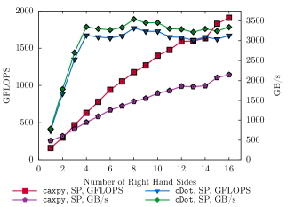
Figure 3: The GFLOPS (left) and GB/s (right) of block caxpy and cDotProduct as a function of the number of right hand sides. Measurements are taken from a $24^{4}$ lattice, in single precision. Block caxpy scales nearly linearly in the number of right hand sides, while the block cDotProduct very quickly saturates cache bandwidth. Tests were performed on a Quadro GP100 GPU.

We see in figure 2 that reductions scale linearly in cost for a much narrower regime of $N$ than the block caxpy operation. This is consistent with what is seen in figure 3. Block reductions quickly saturate cache bandwidth as a function of $N$ and tiling thus becomes essential even for modest numbers of right hand sides. On top of tuning the internal block reduction, we tune the tile size for recursive reductions to be mindful of two different potential optimizations via a policy class. First, we perform distinct tunings for when the left and right block vectors alias versus when they do not. When the two block vectors alias, the subset of reductions on the “block-diagonal” inner tiles feature memory-load reuse. Second, we perform distinct tunings for when the output dense matrix is Hermitian versus when it is not Hermitian. In blockCGrQ, the output dense matrices are always Hermitian, thus we only perform a block reduction on inner tiles (without loss of generality) above the block diagonal. We then reconstruct the inner tiles below the block diagonal by taking advantage of the overall Hermiticity of the matrix. Smaller tile sizes further reduce the total number of redundant calculations. For this reason, it may be beneficial to use a smaller tile size despite an overall increase in memory streaming. This is automatically optimized by policy-class tuning.

We also explored the potential optimization of not computing elements within the inner-block-diagonal tiles below the inner diagonal. However, as this only reduces the number of floating point operations in a tile and does not decrease the overall memory traffic, no benefit was found.

Tuning the tile size is crucial for fully optimizing block reductions. The magnitude of the vector size $L$ leads to different optimal tile sizes. Less threads are used in the case of smaller $L$ and larger tile sizes are needed to saturate memory bandwidth. In contrast, more threads are used in the case of larger $L$, which can saturate the memory bandwidth with smaller tile sizes. The optimal tile size also depends on the precision of the input block vectors. High-precision input vectors will saturate memory bandwidth more quickly than lower-precision input vectors. For this reason, high precision input vectors prefer smaller tile sizes. Low precision input vectors will instead saturate cache load instructions, which also leads to a preference towards smaller tile sizes.

6.5 Benchmarking the implementation

Optimizing the streaming and reduction multi-BLAS kernels to obtain almost linear scaling is a crucial component in our implementation. Without this, the lower iteration count would not translate into a reduced time to solution. In figure 4 we show the time for running 100 iterations of blockCGrQ in double precision.

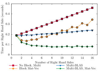
Figure 4: Time for 100 iterations of blockCGrQ. We show the naïve implementation and the effect of adding in the optimized block BLAS routines and also the block-optimized matrix-vector product. Tests were performed on a Quadro GP100 GPU.

For the naïve implementation, “No-Block”, the time per rhs rises linearly as expected from the quadratic scaling of the sequential BLAS-1 operations. Turning on the corresponding BLAS-3 operations is the most important optimization. It brings the time per rhs down to almost constant and a reduced iteration count will almost directly translate to a reduced time to solution. Switching to the version that also enables the block-matrix-vector kernel significantly reduces the time per iteration for a small number of rhs and we see an almost flat behavior between 8 and 16 rhs, at only half of the time of one iteration of a CG solver with 1 rhs. Hence we can expect to see a multiplicative speedup from the block-matrix-vector operation and the reduced iteration count from blockCGrQ.

7 Results

7.1 Methodology

To test the algorithm in the context of the target measurement of the disconnected part of the contribution to the muon $g-2$, we used development versions of the MILC code and QUDA. We compiled using GCC v4.8.5 and the CUDA-toolkit 8.0. The Small and Medium data sets were processed on a workstation equipped with two Quadro GP100 GPUs using MVAPICH2 2.2. The Large and X-Large data sets were run on the NVIDIA SaturnV cluster: each node consists of a DGX-1 server, with eight Tesla P100 GPUs with the NVLink intra-node fabric and a quad EDR Infiniband interconnect between nodes. OpenMPI 1.10.6 was used as the communications layer. We used gauge configurations from an ongoing $g-2$ project, as shown in the following table.

Label	$L_{s}$	$L_{t}$	$a$ (fm)	$m_{\pi}$ (MeV)
Small	16	48	0.15	$\approx 265$
Medium	32	48	0.15	$\approx 133$
Large	48	64	0.12	$\approx 133$
X-Large	64	192	0.06	$\approx 297$

Table 1: Lattice configurations and their physical parameters; the pion mass $m_{\pi}$ roughly corresponds to the quark mass parameter that appears in equation 2.

The goal of our tests is to determine if the optimizations explored in $\S$6 bear fruit when combined in blockCGrQ. As a model test case, we consider stochastic trace estimation for the HISQ stencil given in equation 2. This is a relevant measurement for the $g-2$ project and is also a scenario which necessarily requires a large number of linear solves. In this case, we have a total of 192 rhs per test: 24 noise sources, each partitioned into 8 disjoint subsets. For the 1–2 GPU tests on the Small and Medium datasets, we utilize the Truncated Solver Method (TSM) [49], which consists of a predictor-corrector scheme, partitioning the trace of the inverse matrix into two sweeps: first a cheaper bulk prediction is calculated, at the expense of introducing a bias that must be corrected in a subsequent high precision (fine) computation. The sloppy relative residual was set to $5\times 10^{-6}$, whereas the fine solves used $2\times 10^{-9}$. For simplicity, in our strong scaling tests, we only consider fine solves to a relative tolerance of $2\times 10^{-12}$.

The primary quantity of interest is the total time to iteratively solve $M$ against all 192 rhs. Our baseline is the current CG implementation in QUDA where we sequentially solve on all rhs. For comparison, we perform blockCGrQ in blocks of rhs of size 8, 16, 24, 32, 48, and 64, leading to 24, 12, 8, 6, 4, and 3 applications of blockCGrQ, respectively. We skip some cases as applicable due to insufficient memory or unreasonably small local volumes. We consider both the case of full double precision and a mixed double-single solve to explore the viability, stability, and potential benefits of block reliable updates. We choose to trigger a reliable update when the relative residual drops by a factor of 10. Double-half mixed-precision solves will be a point of future work as noted in $\S$8.

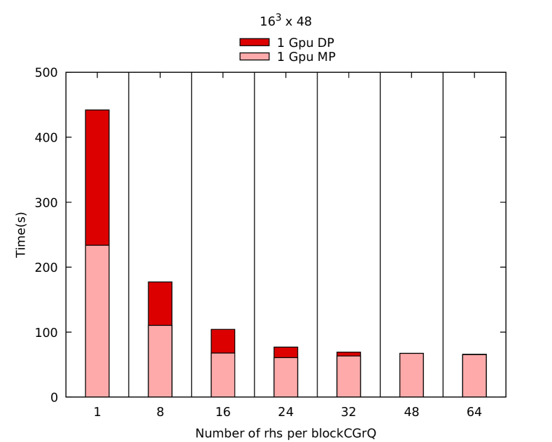
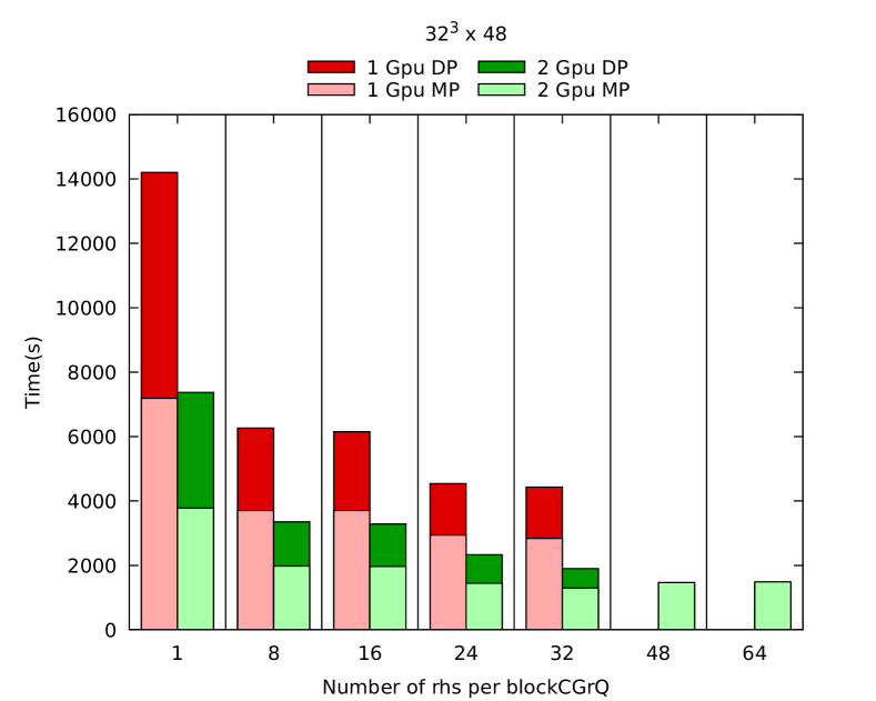
Figure 5: Time to solution for the $16^{3}\times 48$ volume, top, and $32^{3}\times 48$ volume, bottom, as a function of the number of RHS. For a fixed number of RHS, the number of GPUs increases from left to right. When the number of RHS is large enough, the system doesn’t fit in one GPU and only two GPU results are shown. The two GPU cases for 48 and 64 rhs show a consistent time to solution value between double and mixed-precision.

7.2 Results: Single Node

In the single-node case, given the optimizations discussed above, our implementation of blockCGrQ should generally display a monotonic decrease in the complete time to solution for all 192 rhs. An appreciable increase in the time to solution would indicate a remnant quadratic scaling in memory streaming, or, in the case of mixed precision, a breakdown of stability. For smaller block sizes, this is in part due to the reduced total iteration counts due to the sharing of the Krylov space inherent to blockCGrQ, but more importantly because we can better saturate memory bandwidth. For larger block sizes, after fully saturating memory bandwidth, the benefit is near solely from the reduced total iteration count.

This behavior is reflected in figure 5, the total time to solution; figure 6, the average TFLOPS per second; and the green (lowest) and blue (second highest) curves in figure 7, the total number of iterations. The relative reduction in iteration count for a double-precision case is emphasized in figure 8. We see that the total time to solution does indeed monotonically decrease, reaching a 7$\times$ speedup for double precision and 4$\times$ speedup for mixed-precision, although the benefits become less drastic for a larger block size. The drastic speedup for smaller block sizes is largely due to a better utilization of memory bandwidth, as the iteration count does not greatly decrease. After memory bandwidth has saturated, roughly correlated to a saturation in the TFLOPS per second, the benefit comes from a significant reduction in the number of iterations.

We note that the pure-double-precision solve saturates before the double-single-mixed-precision solve: this reflects both a better utilization of streaming memory bandwidth. For intermediate block sizes, this also reflects a stability of the mixed-precision solve. For larger block sizes, the double-precision solve and the mixed-precision solve take a consistent amount of time (48 and 64). This coincides with a slight breakdown in the stability of the mixed-precision solve, where the reduced time per iteration is offset by the relative increase in iteration count. Regardless, it is still slower than the mixed-precision solve at a lower block size (32). It is thus important to appropriately tune the block size; bigger is not necessarily better.

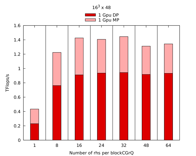
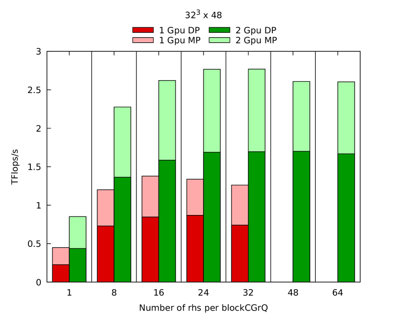
Figure 6: Performance in TFlops/s for the $16^{3}\times 48$ volume, top, and $32^{3}\times 48$ volume, bottom, as a function of the number of rhs. Notation as in figure 5.

7.3 Results: Strong Scaling

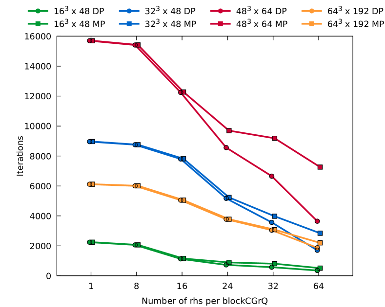
Figure 7: Total iteration count as a function of the number of RHS. The smallest volumes ($16^{3}\times 48$ and $32^{3}\times 48$) show the sum of the sloppy + fine iterations, whereas the larger volumes only show the fine iterations.

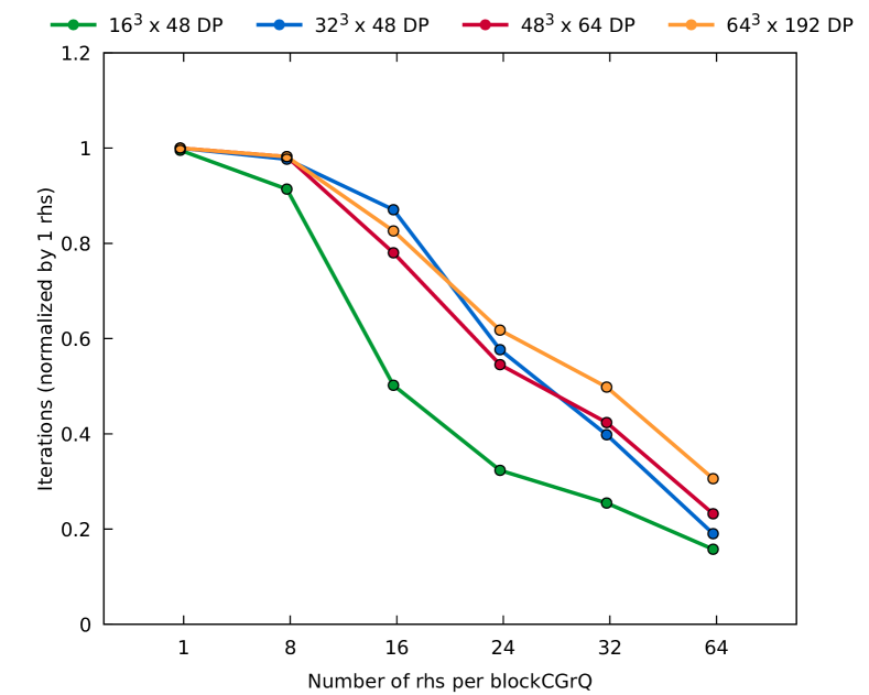
Figure 8: Total iteration count, normalized by the 1 rhs per block case, as a function of the number of RHS. To improve clarity, only the double-precision results are shown.

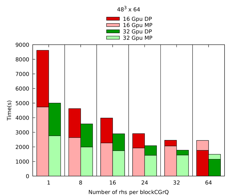
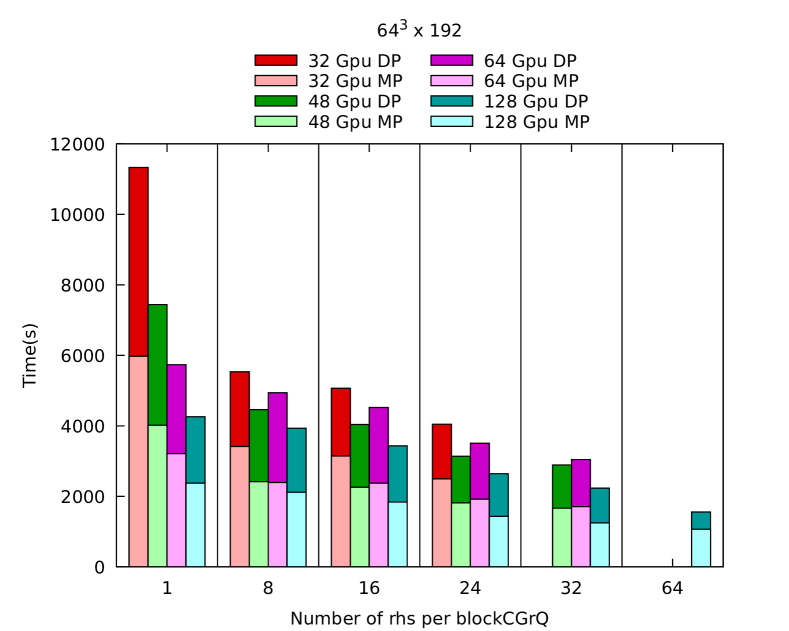
Figure 9: Time to solution for the $48^{3}\times 64$ volume, top, and $64^{3}\times 192$ volume, bottom, as a function of the number of RHS. The number of GPUs for a fixed number of RHS grows from left to right.

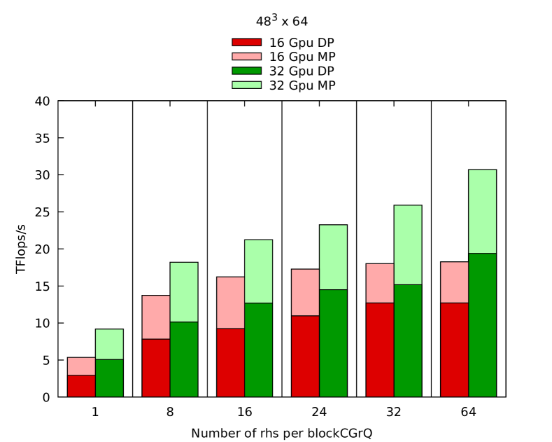
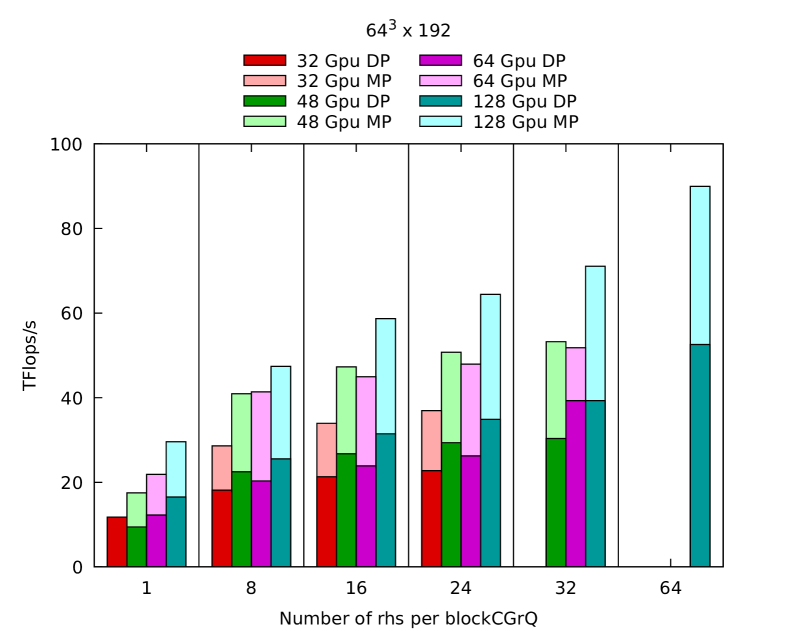
Figure 10: Performance in TFlops/s for the $48^{3}\times 64$ volume, top, and $64^{3}\times 192$ volume, bottom, as a function of the number of RHS. Notation as in figure 9.

In considering the strong-scaling regime of our implementation of blockCGrQ, we ran on the NVIDIA SaturnV cluster. The key features to highlight are that we are able to better utilize the GPUs by overlapping computation with network communications during the matrix-vector operation. In addition, we can reduce the overall number of MPI reductions by simultaneously reducing over multiple rhs as per utilizing blockCGrQ. There is also the subtle benefit that, in cases where the local volume per GPU becomes small, we can still saturate streaming memory bandwidth by sufficiently increasing the block size.

It is difficult to decouple all three of these benefits. However, we can generally comment on the achieved speed-up by again considering figure 9, the total time to solution; figure 10, the average TFLOPS per second; and the yellow (second lowest) and red (highest) curves in figure 7, the total number of iterations. The relative reduction in iteration count for a double-precision case is emphasized in figure 8. We emphasize that, despite corresponding to a larger overall volume, it is not surprising that the X-Large volume (yellow) took far less iterations than the Large volume (red)—the HISQ stencil in the X-Large case is better conditioned than the Large case in one-to-one correspondence with the larger $m_{\pi}$ in table 1. It is more important to consider the relative behavior along the curves.

Our data shows that we achieve an impressive improvement over CG in the strong-scaling regime for a smaller blocksize across both data sets and both precision studies. This is, in some sense, reflective of both the single-node optimizations and the additional strong-scaling benefits. In the case of the X-Large measurement set, the TFLOPS per second monotonically increases with both the number of rhs and the number of GPUs. This may be from a combination of there being increasing work to overlap with communications and additional memory bandwidth to saturate with smaller local volumes (especially in the mixed-precision case). This suggests that, given the resources, the algorithm would continue to strong scale well. The relatively low iterations count corresponds to a relative well-conditioning of the HISQ stencil on the X-Large data set: an increased blocksize always leads to a reduction in the number of iterations.

We see a smaller benefit for the Large measurement set, where in some cases the TFLOPS per second saturates. This could be due to a saturation of memory bandwidth on a local node combined with network latency being hidden behind computation, which in some regards indicates we can strong scale ideally. For very large block sizes there is an increase in the time to solution in the mixed-precision case: this is likely due to a decreased stability in the mixed-precision case. However, in all cases, there is an ideal number of rhs where we can minimize the total time to solution, and for our X-Large data set, that ideal pushes the maximum blocksize and strong-scaling limit we can achieve with our current tests.

In the end the benefits translate into a 2-3$\times$ speedup factor for the mixed double-single precision solver, and a 4-5$\times$ speedup factor for double precision, compared to the baseline.

8 Future Work

Our initial implementation of blockCGrQ overcomes many of the traditional issues which stifled the development and use of block-Krylov methods. There are several low-hanging fruit that can extend the application of blockCGrQ in its current form that may be of interest. For example, deflation methods, or any other method which improves the initial guess to a linear system, can be trivially combined with block-Krylov methods.

There are more advanced algorithmic pursuits that can be considered. As the Lanczos method is closely related to CG, there is an analogous block-Lanczos method that is related to block CG. At this time, we do not know if a Lanczos relation can be easily recovered from the modifications made in blockCGrQ, but if possible it may allow for the development of a block analogy to the EigCG [9] which generates and iteratively improves a deflation space along the course of a Krylov solve without any additional stencil applications.

There are further improvements possible within the scope of our current work. One novel development in this work was the implementation of reliable updates [19] in a block-Krylov method. While this was successful in the case of stabilizing a full double-precision solve as well as a mixed-precision double-single solve with a modestly sized number of rhs, our implementation of reliable updates broke down for double-single with a large number of rhs and completely broke down for a double-half mixed-precision solve. There are more advanced reliable-update methods in the literature for non-block-Krylov methods, which could potentially be generalized for block-Krylov methods. A stable implementation with half precision would significantly speed up portions of blockCGrQ that are still memory bandwidth bound. It would also speed up the matrix-vector portions of the algorithm because the HISQ stencil could now be applied in low precision. Last, it would reduce the overall memory footprint which can be the limiting factor when running at low-node count.

Further improvement to the strong scaling would likely be possible through utilizing s-step solver methods which reduce the number of reductions to less than one per solver iteration. These have been deployed previously for block solvers to improve parallel scaling [50], and such algorithms could easily be accomodated for in the context of our block-solver framework. Given that s-step solvers are typically less numerically stable, we expect that it will be essential to first develop better reliable-update methods for blockCGrQ.

As a last note, other non-block-Krylov methods have block-Krylov extensions. The technology we have developed for an efficient implementation of blockCGrQ, i.e. block-optimized stencil operations and multi-BLAS operations, are immediately applicable to other block-Krylov methods.

9 Conclusions

In this paper we revisited the blockCGrQ solver proposed in [2]. We present an implementation that, by exploiting data locality for reductions and streaming multi-BLAS operation, reduces the naïve quadratic scaling of memory traffic to almost linear scaling. Using a block-optimized matrix-vector operation we obtain a speedup that multiplicatively combines with the reduced iteration count from the blockCGrQ algorithm. With its increased parallelism it is an algorithm very well suited also for future exascale machines where we expect the gap between peak floating point operations per seconds and memory bandwidth will continue to increase. We have also laid the groundwork and demonstrated the algorithm working using mixed precision, a further important building block for efficient algorithms. In our real world LQCD use case we demonstrated a speedup of 5$\times$, notably not requiring any overhead from setup and also not requiring large storage for precalculated inputs such as eigenvectors. The availability of the building blocks for an efficient implementation of blockCGrQ can be employed with new algorithms, in order to improve lattice field theory computational methods to allow new physics research. Precision results in LQCD are already competing in accuracy with the best experimental results, but in a lot of areas computational demands are still the limiting factor.

Although we employed lattice QCD as one use case, we again emphasize that the problem of efficiently solving a sparse matrix linear system over multiple rhs is a quite general one that appears in many disciplines. The key features of the implementation that make our BlockCGrQ solver efficient are generic and transfering them to other applications or libraries is expected to be straightforward.

References

References

- [1] A. A. Nikishin, A. Y. Yeremin, SIAM J. Matrix Anal. A. 16 (4) (1995) 1135–1153.
- [2] A. Dubrulle, Electron. T. Numer. Ana. 12 (2001) 216–233.
- [3] M. A. Clark, R. Babich, K. Barros, R. C. Brower, C. Rebbi, Comput. Phys. Commun. 181 (2010) 1517–1528. arXiv:0911.3191.
- [4] M. Clemens, M. Helias, T. Steinmetz, G. Wimmer, J. Comput. Appl. Math. 215 (2008) 328–338.
- [5] V. Puzyrev, J. M. Cela, Geophys. J. Int. 202 (2) (2015) 1241–1252.
- [6] F. X. Roux, A. Barka, IEEE T. Antenn. Propag. 65 (4) (2017) 1886–1895.
- [7] B. Krasnopolsky, Simultaneous modelling of multiple turbulent flow states (Nov. 2017). arXiv:1711.10622.
- [8] Y. Wang, M. Baboulin, K. Rupp, O. Le Maître, Y. Fraigneau, Solving 3d incompressible navier-stokes equations on hybrid cpu/gpu systems, in: Proceedings of the High Performance Computing Symposium, HPC ’14, Society for Computer Simulation International, San Diego, CA, USA, 2014, pp. 12:1–12:8.
- [9] A. Stathopoulos, K. Orginos, SIAM J. Sci. Comput. 32 (1) (2010) 439–462.
- [10] W. M. Wilcox, PoS LAT2007 (2007) 025. arXiv:0710.1813.
- [11] J. Brannick, R. C. Brower, M. A. Clark, J. C. Osborn, C. Rebbi, Phys. Rev. Lett. 100 (2008) 041601. arXiv:0707.4018.
- [12] R. Babich, et al., Phys. Rev. Lett. 105 (2010) 201602. arXiv:1005.3043.
- [13] M. Lüscher, JHEP 07 (2007) 081. arXiv:0706.2298.
- [14] H. Calandra, S. Gratton, J. Langou, X. Pinel, X. Vasseur, SIAM J. Sci. Comput. 34 (2) (2012) A714–A736.
- [15] P. Jolivet, P.-H. Tournier, Block iterative methods and recycling for improved scalability of linear solvers, in: Proceedings of the International Conference for High Performance Computing, Networking, Storage and Analysis, SC ’16, IEEE Press, Piscataway, NJ, USA, 2016, pp. 17:1–17:14.
- [16] E. Bavier, M. Hoemmen, S. Rajamanickam, H. Thornquist, Sci. Program. 20 (3) (2012) 241–255.
- [17] H. Ji, M. Sosonkina, Y. Li, An implementation of block conjugate gradient algorithm on cpu-gpu processors, in: Proceedings of the 1st International Workshop on Hardware-Software Co-Design for High Performance Computing, Co-HPC ’14, IEEE Press, Piscataway, NJ, USA, 2014, pp. 72–77.
- [18] H. Ji, Y. Li, BIT Numerical Mathematics 57 (2) (2017) 379–403.
- [19] H. A. van der Vorst, Q. Ye, SIAM J. Sci. Comput. 22 (3) (2000) 835–852.
- [20] G. I. Egri, Z. Fodor, C. Hoelbling, S. D. Katz, D. Nógrádi, K. K. Szabó, Comp. Phys. Commun. 177 (8) (2007) 631 – 639. arXiv:0611022.
- [21] R. Babich, M. A. Clark, B. Joó, Parallelizing the QUDA Library for Multi-GPU Calculations in Lattice Quantum Chromodynamics, in: Proceedings of the 2010 ACM/IEEE International Conference for High Performance Computing, Networking, Storage and Analysis, SC ’10, IEEE Computer Society, Washington, DC, USA, 2010, pp. 1–11. arXiv:1011.0024.
- [22] G. Shi, S. Gottlieb, A. Torok, V. V. Kindratenko, Design of MILC lattice QCD application for GPU clusters, in: IPDPS, IEEE, 2011.
- [23] A. Alexandru, M. Lujan, C. Pelissier, B. Gamari, F. X. Lee, Efficient implementation of the overlap operator on multi- GPUs (2011). arXiv:1106.4964.
- [24] R. Babich, M. A. Clark, B. Joo, G. Shi, R. C. Brower, S. Gottlieb, Scaling Lattice QCD beyond 100 GPUs, in: SC11 International Conference for High Performance Computing, Networking, Storage and Analysis Seattle, Washington, November 12-18, 2011, 2011. arXiv:1109.2935.
- [25] M. A. Clark, B. Joó, A. Strelchenko, M. Cheng, A. Gambhir, R. C. Brower, Accelerating lattice qcd multigrid on gpus using fine-grained parallelization, in: Proceedings of the International Conference for High Performance Computing, Networking, Storage and Analysis, SC ’16, IEEE Press, Piscataway, NJ, USA, 2016, pp. 68:1–68:12.
- [26] R. Babich, M. A. Clark, High-efficiency Lattice QCD computations on the Fermi architecture, Innovative Parallel Computing (InPar), 2012.
- [27] R. G. Edwards, B. Joó, Nucl. Phys. Proc. Suppl. 140 (2005) 832. arXiv:hep-lat/0409003.
- [28] F. T. Winter, M. A. Clark, R. G. Edwards, B. Joó, A Framework for Lattice QCD Calculations on GPUs, 2014. arXiv:1408.5925.
- [29] D. P. O’Leary, Linear Algebra Appl. 29 (1980) 293–322.
- [30] T. Sakurai, H. Tadano, Y. Kuramashi, Comput. Phys. Commun. 181 (1) (2010) 113 – 117.
- [31] H. Tadano, Y. Kuramashi, T. Sakurai, Comput. Phys. Commun. 181 (2010) 883. arXiv:0907.3261.
- [32] Y. Nakamura, K. I. Ishikawa, Y. Kuramashi, T. Sakurai, H. Tadano, Comput. Phys. Commun. 183 (2012) 34–37. arXiv:1104.0737.
- [33] S. Birk, A. Frommer, PoS LATTICE2011 (2011) 027. arXiv:1205.0359.
- [34] S. Birk, A. Frommer, Numer. Algorithms 67 (3) (2014) 507–529.
- [35] O. Kaczmarek, C. Schmidt, P. Steinbrecher, M. Wagner, Conjugate gradient solvers on Intel Xeon Phi and NVIDIA GPUs, in: Proceedings, GPU Computing in High-Energy Physics (GPUHEP2014): Pisa, Italy, September 10-12, 2014, 2015, pp. 157–162. arXiv:1411.4439.
- [36] S. Mukherjee, O. Kaczmarek, C. Schmidt, P. Steinbrecher, M. Wagner, PoS LATTICE2014 (2015) 044. arXiv:1409.1510.
- [37] K. Bitar, A. D. Kennedy, R. Horsley, S. Meyer, P. Rossi, Nucl. Phys. B313 (1989) 348–376.
- [38] J. Kogut, L. Susskind, Phys. Rev. D 11 (1975) 395–408.
- [39] E. Follana, Q. Mason, C. Davies, K. Hornbostel, P. Lepage, H. Trottier, Nucl. Phys. Proc. Suppl. 129 (2004) 447–449, [,447(2003)]. arXiv:hep-lat/0311004.
- [40] M. R. Hestenes, E. Stiefel, Journal of Research of the National Bureau of Standards 49 (6) (1952) 409–436.
- [41] C. Bernard, et al., The MILC Code, http://www.physics.utah.edu/~detar/milc/milcv7.pdf (2010).
- [42] http://lattice.github.com/quda (2017).
- [43] T. Fukaya, Y. Nakatsukasa, Y. Yanagisawa, Y. Yamamoto, Choleskyqr2: A simple and communication-avoiding algorithm for computing a tall-skinny qr factorization on a large-scale parallel system, in: 2014 5th Workshop on Latest Advances in Scalable Algorithms for Large-Scale Systems, 2014, pp. 31–38.
- [44] Y. Yamamoto, Y. Nakatsukasa, Y. Yanagisawa, T. Fukaya, JSIAM Letters 8 (2015) 5–8.
- [45] G. H. Golub, C. F. Van Loan, Matrix Computations, 3rd Edition, Johns Hopkins Studies in the Mathematical Sciences, 1996.
- [46] http://eigen.tuxfamily.org (2017).
- [47] G. L. G. Sleijpen, H. A. van der Vorst, Computing 56 (2) (1996) 141–163.
- [48] D. Merrill, CUB, https://nvlabs.github.io/cub (2016).
- [49] G. S. Bali, S. Collins, A. Schafer, Comput. Phys. Commun. 181 (2010) 1570–1583. arXiv:0910.3970.
- [50] C. A. T., K. A. B., Numerical Linear Algebra with Applications 17 (1) (2010) 3–15. arXiv:https://onlinelibrary.wiley.com/doi/pdf/10.1002/nla.643.