Destruction of Axion Miniclusters in the Galaxy

Abstract

Previously, it has been established that axion dark matter (DM) is clustered to form clumps (axion miniclusters) with masses $M\sim 10^{-12}M_{\odot}$. The passages of such clumps through the Earth are very rare events occurring once in $10^{5}$ years. It has also been shown that the Earth’s passage through DM streams, which are the remnants of clumps destroyed by tidal gravitational forces from Galactic stars, is a much more probable event occurring once in several years. In this paper we have performed details calculations of the destruction of miniclusters by taking into account their distribution in orbits in the Galactic halo. We have investigated two DM halo models, the Navarro-Frenk-White and isothermal density profiles. Apart from the Galactic disk stars, we have also taken into account the halo and bulge stars. We show that about 2-5% of the axion miniclusters are destroyed when passing near stars and transform into axion streams, while the clump destruction efficiency depends on the DM halo model. The expected detection rate of streams with an overdensity exceeding an order of magnitude is 1-2 in 20 years. The possibility of detecting streams by their tidal gravitational effect on gravitational-wave interferometers is also considered.

1 INTRODUCTION

Although dark matter (DM) accounts for $\simeq 27$% of the mass of the Universe, its nature still remains unknown. As yet undetected elementary particles are considered as a probable candidate, and a number of specific candidate particles, such as, for example, neutralinos, sterile neutrinos, or axions, have been proposed in theoretical works. The axion field was initially introduced in particle physics to explain the absence of CP violation in strong interactions. The quanta of this field, axions, turned out to be promising candidates for DM particles. Although the axions are expected to have small masses, they belong to the type of cold DM, because their production mechanism is nonthermal; they were not in chemical and kinetic equilibrium with the cosmic plasma.

The existence of DM clumps consisting of axions, axion miniclusters, was predicted in KolTka94 . The clumps are formed due to strong fluctuations of the axion field in various regions of space on the horizon scale at the epoch when the axion oscillations began. The fraction of DM in the form of axion miniclusters is $f_{\rm mc}\sim 1$.

A new effect that could increase the chances of detecting the axion DM passing through the Earth was presented in TinTkaZio16 . It was shown in TinTkaZio16 that although the passage of a whole clump is an extremely rare event, some of the clumps in the Galactic halo are destroyed when interacting with stars, and DM streams with a large overdensity from the destroyed clumps can be observed in ground-based detectors approximately once in 20 years. However, a simplified calculation was performed in TinTkaZio16 . In particular, the orbital motion of clumps and their distribution in orbits were disregarded.

The orbits of clumps in the Galactic halo are not circular but, as a rule, eccentric. The clumps have some distribution in their orbital parameters, with their orbits undergoing precession (see BerDokEro07 , BerDokEro08 ). If a clump or its stream is now passing through the Solar system, then it could previously pass closer to the Galactic center, where the number density of stars is larger and the destruction probability is higher. Therefore, it is necessary to consider the passages through the Galactic disk not only in the solar neighbourhood, as was done in TinTkaZio16 , but also at other distances throughout the entire life history of the clump in the Galactic halo. The goal of this paper is to perform such a calculation. The calculation technique used here is similar to that applied in BerDokEro06 , BerDokEro07 , BerDokEro08 . In this paper we also take into account the halo and bulge stars, which contribute noticeably to the destruction of clumps.

The DM density and velocity in the Galactic halo in the solar neighbourhood are largely fixed by the observational data on the distribution and motion of stars, because DM and baryons move in the same gravitational potential. Nevertheless, there exists some freedom in the choice of halo parameters, and the observational data are compatible with various DM halo models. To ascertain the dependence of the final results on the halo model, we will perform calculations for two distributions of DM particles and DM clumps in the halo in their orbital parameters: the Navarro-Frenk-White and isothermal density profiles. The Galactic halo model turned out to affect noticeably the result.

In this paper we use the characteristic parameters of clumps from KolTka94 in our calculations: the clump mass $M=10^{-12}M_{\odot}$, the mean density $\bar{\rho}=140\rho_{\rm eq}\Phi^{3}(1+\Phi)$, where $\Phi$ are the initial entropy density perturbations in the medium of axions (for more details, see KolTka94 ), at $\Phi=1$ the clump radius is then $R=2.3\times 10^{12}$ cm, while the DM particle velocity dispersion in the clump is $v_{\rm mc}\simeq(GM/R)^{1/2}\simeq 7.6$ cm s^-1 ($v_{\rm mc}/c\simeq 2.5\times 10^{-10}$). We will choose the clump density profile in accordance with the theory of multistream instability ufn1 :

$$\rho_{\rm int}(r)=\frac{3-\beta}{3}\,\bar{\rho}\left(\frac{r}{R}\right)^{-\beta}.$$ (1)

where $\beta=1.7-1.9$ (below in the calculations we set $\beta=1.8$).

2 DESTRUCTION OF CLUMPS AND ADIABATIC PROTECTION

A DM clump is destroyed if the net change in its internal energy $\sum(\Delta E)_{j}$) after one or more gravitational interactions with disk stars or field is comparable to the binding energy of the clump $|E|$:

$$\sum\limits_{j}(\Delta E)_{j}\sim|E|,$$ (2)

where the summation is over the successive gravitational interactions. In reality, the destruction occurs not at once but there is a gradual mass loss predominantly through the tidal stripping of outer DM layers gnedin2 ; TayBab01 ; DieKuhMad ; ZTSH ; GoeGneMooDieSta07 . In this case, the central dense cores of the clumps can survive BerDokEro08 .

If the internal revolution frequencies of DM particles in their orbits inside the clump $\omega=v_{\rm mc}/R$ are much higher than the characteristic frequency of the external tidal force $\tau^{-1}$ (the reciprocal of the passage time through the disk or the reciprocal of the passage time of the impact parameter l to the star), then the influence of the tidal force weakens significantly. This effect is characterized by the so-called adiabatic correction or the Weinberg correction $A(a)$, where $a=\omega\tau$, that is defined as the ratio of the energy change in the real case to the energy change calculated in the impulse approximation Wein1 . The following approximate formula was found in gnedin2 :

$$A(a)=(1+a^{2})^{-3/2}.$$ (3)

The Galactic disk consists of stars and gas. The destruction of clumps includes both the interaction with the collective disk field and the interaction with individual stars that happen to be near the clump trajectory in the halo. In the former case, the tidal gravitational field is produced not only by the disk stars but also by the gas-dust clouds in the disk, i.e., by the total gravitating disk mass.

Let us first consider the interaction of clumps with the collective gravitational field of the disk when $\tau\simeq H_{d}/v$, where $H_{d}\sim 500$ pc is the Galactic disk halfthickness and $v\sim 200$ km s^-1 is the characteristic passage velocity. Whereas for neutralino clumps $a\sim 1$ BerDokEro08 , for axion clumps $a\sim 200$. Thus, in the latter case, the clump destruction effect is suppressed approximately by three orders of magnitude. The estimate made in the impulse approximation shows that the destruction time of axion miniclusters by the collective disk field is $\sim 10^{15}$ years. If the adiabatic correction is taken into account, then this time increases to $\sim 10^{18}$ years. Thus, this destruction channel is inefficient, and during the passage of axion clumps through the disk only the interactions with individual stars are important, while the gravitational shocks by the collective disk field play no role.

During the interactions with individual stars $\tau\sim l/v$. Let us take the maximum impact parameter at which the clump is destroyed in a single star flyby BerDokEro06 as $l$:

$$\left(\frac{l_{*}}{R}\right)^{4}=\frac{4(5-2\beta)}{3(5-\beta)}\frac{Gm_{*}^{2}}{MRv_{\rm rel}^{2}},$$ (4)

where $v_{\rm rel}$ is the relative velocity of the clump and the star, and $m_{*}$ is the mass of the star. For the typical parameters of clumps given at the end of the Introduction and at $\beta\simeq 2$, $v_{\rm rel}$=200 km s^-1, $m_{*}\sim M_{\odot}$ we obtain $l_{*}\sim 500R$ and $a\sim 10^{-4}$, i.e., in typical cases, during the interactions with stars the adiabatic correction is unimportant and will be disregarded below.

3 DESTRUCTION OF CLUMPS IN GRAVITATIONAL COLLISIONS WITH STARS

In BerDokEro06 the characteristic destruction time of a clump as it moves in a medium of stars with number density $n_{*}$ and mass $m_{*}$ was found for the case of $l_{*}/R>1$:

$$t_{*}=\frac{|E|}{\dot{E}}=\frac{1}{4\pi n_{*}m_{*}}\left[\frac{3(5-\beta)}{(5-2\beta)}\frac{M}{GR^{3}}\right]^{1/2}.$$ (5)

Note that at $l_{*}/R>1$ the destruction time (5) does not depend on the relative velocity of the clump and the stars.

The survival probability of some specific clump

$$P_{1}=e^{-\int dt/t_{*}}$$ (6)

depends on its trajectory; therefore, we will first determine the parameters of the clump trajectories in the Galactic halo needed for the subsequent discussion in a general form.

3.1 The Trajectories of Clumps in the Galactic Halo

Let us denote the orbital angular momentum of a clump by $J$. The equation of the trajectory for $r(t)$ is then

$$M\dot{r}^{2}={2}\left[E_{\rm orb}-U(r)\right]-\frac{J^{2}}{Mr^{2}},$$ (7)

where $U(r)$ is the potential energy of the clump in the halo. In what follows, we will consider an isotropic distribution of clump orbits in the halo with a total orbital energy $E_{\rm orb}$ (not to be confused with the internal energy $E$) distribution function $F(E_{\rm orb})$ when the relation to the halo density $\rho_{\rm H}(r)$ is given by the expressions Edd16

$$\rho_{\rm H}(r) = 2^{5/2}\pi\int\limits^{0}_{U(r)}\sqrt{E_{\rm orb}-U(r)}F(E_{\rm orb})dE_{\rm orb},$$ (8)

$$F(E_{\rm orb}) = \frac{1}{2^{3/2}\pi^{2}}\frac{d}{dE_{\rm orb}}{\int\limits_{r(E_{\rm orb})}^{\infty}}\frac{dr}{\sqrt{E_{\rm orb}-U(r)}}\frac{d\rho_{\rm H}(r)}{dr},\;$$ (9)

where the function $r=r(E_{\rm orb})$ is found from the equation $U[r(E_{\rm orb})]=E_{\rm orb}$.

For the convenience of our subsequent discussion, let us introduce the following dimensionless variables:

$$\xi=\frac{r}{R_{c}},\quad\tilde{\rho}(\xi)=\frac{\rho_{\rm H}^{\leavevmode\nobreak\ }(r)}{\rho_{0}},\quad y=\frac{J^{2}}{2MU_{0}R_{c}^{2}},$$ (10)

$$\varepsilon=\frac{E_{\rm orb}}{U_{0}},\quad\psi=\frac{U}{U_{0}},$$ (11)

where $U_{0}$, $\rho_{0}$, and $R_{c}$ are some characteristic values of the gravitational potential, the density, and the radius in a specific DM halo model. In what follows, we will choose these parameters so that $U_{0}=4\pi G\rho_{0}R_{c}^{2}M$.

The equation of the clump trajectory for the azimuthal angle $\phi(\xi)$ is

$$\frac{d\phi}{d\xi}=\frac{y^{1/2}}{\xi^{2}\sqrt{\varepsilon-\psi(\xi)-y/\xi^{2}}}.$$ (12)

The equation for the extreme points of the orbit $\dot{r}^{2}=0$ will be written as

$$\frac{y}{\xi^{2}}=\varepsilon-\psi.$$ (13)

In our calculations we then numerically find the roots of this equation $\xi_{\rm min}$ and $\xi_{\rm max}$. Twice the time of clump motion from $\xi_{\rm min}$ to $\xi_{\rm max}$

$$T_{c}(\varepsilon,y)=\frac{1}{\sqrt{2\pi G\rho_{0}}}\int\limits_{\xi_{\rm min}}^{\xi_{\rm max}}\frac{d\xi}{\sqrt{\varepsilon-\psi(\xi)-y/\xi^{2}}}$$ (14)

is not equal to the orbital period, because the orbital precession should be additionally taken into account. The precession angle in the time $T_{\rm c}/2$ is

$$\tilde{\phi}=y^{1/2}\int\limits_{\xi_{\rm min}}^{\xi_{\rm max}}\frac{d\xi}{\xi^{2}\sqrt{\varepsilon-\psi(\xi)-y/\xi^{2}}}-\pi,$$ (15)

and $\tilde{\phi}<0$. Therefore, the true period (the revolution around the Galactic center through $2\pi$) is

$$T_{\rm t}=T_{\rm c}\left(1+\tilde{\phi}/\pi\right)^{-1}.$$ (16)

Below we consider the clumps whose orbits are currently passing through the Solar system at a distance $r=r_{\odot}=8.5$ kpc from the Galactic center. Denote $p=\cos\theta$, where $\theta$ is the angle between the radius vector of the clump $\vec{r}$ and its velocity $\vec{v}$ in the solar neighborhood. The dimensionless parameter $y$ characterizing the angular momentum of the clump can then be found from the expression

$$y=(1-p^{2})\xi^{2}\left[\varepsilon-\psi(\xi)\right],$$ (17)

where we should set $\xi=r_{\odot}/R_{c}$.

3.2 Destruction of Clumps by Disk Stars

In the lifetime of the Galaxy $t_{\rm G}\simeq 10^{10}$ years a clump experiences $N\simeq t_{\rm G}/T_{\rm t}$ double crossings of the Galactic disk, with the crossing points every time being shifted by angles $|\tilde{\phi}|$ due to the precession effect.

The survival probability (6) of some specific clump contains the integral

$$\int m_{*}n_{*}\leavevmode\nobreak\ dt\simeq\sum\int\frac{m_{*}n_{*}dl}{v},$$ (18)

where the summation is over the successive Galactic disk crossings in the time $t_{\rm G}$, while the integration is over one specific crossing. This integral is expressed via the mass surface density $\sigma_{s}$ of the stellar component of the Galactic disk,

$$\int\frac{m_{*}n_{*}dl}{v}=\frac{\sigma_{s}}{v_{z}},$$ (19)

while the distribution of stars in masses $m_{*}$ does not enter into the result. The clump velocity component along the normal to the disk is written as

$$v_{z}=\frac{J}{r}\sin\gamma,$$ (20)

where $\gamma$ is the angle between the normal to the orbital plane and the normal to the Galactic disk plane. The surface density of the stellar component of the Galactic disk at point $r$ of its crossing by the clump is given by the expression

$$\sigma_{s}(r)=\frac{M_{d}}{2\pi r_{0}^{2}}\,e^{-r/r_{0}},$$ (21)

where $M_{d}=3\times 10^{10}M_{\odot}$ and $r_{0}=4.5$ kpc, so that $\sigma_{s}(r_{\odot})=35M_{\odot}$ pc^-2. Here, we take into account the fact that the stars constitute only part of the total disk mass. The normalization $\sigma_{s}(r_{\odot})=35M_{\odot}$ pc^-2 corresponding to the stars was taken from KuiGil89 (page 635).

The orbital precession effect facilitates considerably the calculation of the sum in Eq. (18), because the clump successively crosses the disk at equal angular intervals at all radii between the minimum and maximum radial distances of the orbit owing to the precession. Therefore, we approximately calculate the sum as follows:

$$\sum\limits_{i=1}^{N}\sigma_{s}(r)r\simeq\frac{1}{|\tilde{\phi}|}\int\sigma_{s}R_{c}\xi d\phi\simeq\frac{R_{c}}{|\tilde{\phi}|}\int\limits_{\xi_{\rm min}}^{\xi_{\rm max}}\sigma_{s}(\xi)\xi\frac{d\phi}{d\xi}d\xi\frac{2t_{\rm G}}{T_{\rm t}},$$

Let us rewrite (6) as

$$P_{1}=\exp\left\{-\frac{\lambda}{\Phi^{3/2}(1+\Phi)^{1/2}\sin\gamma}\right\},$$ (22)

where

$$\lambda=2(2\pi)^{1/2}\left(\frac{5-2\beta}{5-\beta}\right)^{1/2}\frac{G^{1/2}t_{\rm G}S}{T_{\rm t}|\tilde{\phi}|(140\rho_{\rm eq})^{1/2}U_{0}^{1/2}},$$ (23)

$$S=\int\limits_{\xi_{\rm min}}^{\xi_{\rm max}}\frac{d\xi\sigma_{s}(\xi)}{\xi\sqrt{\varepsilon-\psi(\xi)-y/\xi^{2}}}.$$ (24)

Using (14), we obtain the fraction of destroyed clumps in the solar neighbourhood:

$$P=1-\frac{\int\limits_{0}^{1}dp\int\limits_{0}^{\sin\alpha}d\cos\gamma\int\limits_{\psi(\xi)}^{0}d\varepsilon[\varepsilon-\psi(\xi)]^{1/2}F(\varepsilon)P_{1},}{\int\limits_{0}^{1}dp\int\limits_{0}^{\sin\alpha}d\cos\gamma\int\limits_{\psi(\xi)}^{0}d\varepsilon[\varepsilon-\psi(\xi)]^{1/2}F(\varepsilon),}$$ (25)

where we should substitute $\xi=r_{\odot}/R_{c}$ and $\alpha\approx\pi/2$.

3.3 Destruction of Clumps by Halo and Bulge Stars

Outside the Galactic disk there are stars of the spherical subsystems: these are halo and bulge stars (plus stars in globular clusters, which we disregard). The number density of stars in the halo at a distance $r>3$ kpc from the Galactic center is

$$n_{h,*}(r)=(\rho_{\odot}/m_{*})(r_{\odot}/r)^{3},$$ (26)

where we took $\rho_{\odot}=10^{-4}\leavevmode\nobreak\ M_{\odot}/$pc³ as an estimate. Note, however, that an order of magnitude larger value, $\rho_{\odot}=10^{-3}\leavevmode\nobreak\ M_{\odot}/$pc³, is obtained in some studies (see ColOst81 and references in ColOst81 , MarSuch ). However, the authors of MDSQ2 point out that even $\rho_{\odot}=10^{-4}\leavevmode\nobreak\ M_{\odot}/$pc³ should be considered as an upper limit for the density of stars in the halo.

The number density of stars in the bulge at a distance $r=1-3$ kpc LauZylMez is

$$n_{b,*}(r)=(\rho_{b}/m_{*})\exp\left[-(r/r_{b})^{1.6}\right],$$ (27)

where ?$\rho_{b}=8M_{\odot}/$pc³ and $r_{b}=1$ kpc.

For our calculations we will need to sum the clump energy change over the orbital period or, which is mathematically equivalent, to average $t^{-1}_{*}$ over the clump trajectory in the halo:

$$\langle t_{*}^{-1}\rangle=\frac{R_{c}}{T_{c}}\sqrt{\frac{2}{U_{0}}}\int\limits_{\xi_{\rm min}}^{\xi_{\rm max}}\frac{t_{*}^{-1}d\xi}{\sqrt{\varepsilon-\psi(\xi)-y/\xi^{2}}}.$$ (28)

The survival probability of a single clump is

$$P_{1}=e^{-t_{\rm G}\langle t_{*}^{-1}\rangle}=\exp\left\{-\frac{\lambda}{\Phi^{3/2}(1+\Phi)^{1/2}}\right\},$$ (29)

where, in the case under consideration,

$$\lambda=2(2\pi)^{1/2}\left(\frac{5-2\beta}{5-\beta}\right)^{1/2}\frac{R_{c}m_{*}G^{1/2}t_{\rm G}S}{T_{\rm c}(140\rho_{\rm eq})^{1/2}U_{0}^{1/2}},$$ (30)

$$S=\int\limits_{\xi_{\rm min}}^{\xi_{\rm max}}\frac{d\xi n_{s}(\xi)}{\sqrt{\varepsilon-\psi(\xi)-y/\xi^{2}}}.$$ (31)

Owing to the presumed spherical symmetry of the halo and the bulge, the expression for the fraction of destroyed clumps is simplified:

$$P=1-\frac{\int\limits_{0}^{1}dp\int\limits_{\psi(\xi)}^{0}d\varepsilon[\varepsilon-\psi(\xi)]^{1/2}F(\varepsilon)P_{1}}{\int\limits_{0}^{1}dp\int\limits_{\psi(\xi)}^{0}d\varepsilon[\varepsilon-\psi(\xi)]^{1/2}F(\varepsilon)}.$$ (32)

4 DESTRUCTION OF CLUMPS IN THE NAVARRO-FRENK-WHITE HALO MODEL

Let us first calculate the destruction of axion miniclusters for the Navarro-Frenk-White density profile

$$\rho_{\rm H}(r)=\frac{\rho_{0}}{(r/R_{c})(1+r/R_{c})^{2}},$$ (33)

where $\rho_{\rm H}(r_{\odot})=0.3$ GeV/cm³ and $R_{c}=20$ kpc. It should be noted that a density profile close in shape to the Navarro-Frenk-White profile was obtained in the analytical model SikTkaWan96 .

The halo density in dimensionless variables is

$$\tilde{\rho}(\xi)=\frac{1}{\xi(1+\xi)^{2}}.$$ (34)

Choosing $U_{0}=4\pi G\rho_{0}R_{c}^{2}$, we find the gravitational potential in dimensionless variables:

$$\psi(\xi)=-\frac{\log(1+\xi)}{\xi}.$$ (35)

The distribution function $F(\varepsilon)$ for the profile (34) was approximated in Wid00 by the expression

$$F(\varepsilon)=F_{1}(-\varepsilon)^{3/2}(1+\varepsilon)^{-5/2}\left[-\frac{\ln(-\varepsilon)}{(1+\varepsilon)}\right]^{q}e^{P},$$ (36)

where $F_{1}=9.1968\times 10^{-2}$, $P=\sum\limits_{i}p_{i}(-\varepsilon)^{i}$, $(q{,}p_{1}{,}p_{2}{,}p_{3}{,}p_{4})=(-2.7419{,}0.3620{,}-0.5639{,}-0.0859{,}-0.4912)$. Then,

$$\tilde{\rho}(\xi)=4\pi\sqrt{2}\int\limits_{\psi(\xi)}^{0}d\varepsilon\left[\varepsilon-\psi(\xi)\right]^{1/2}F(\varepsilon).$$ (37)

The fraction of clumps in the solar neighbourhood destroyed in their collisions with stars (25) found by numerically calculating all of the integrals in it is indicated by the circles in Fig. 1 for various values of $\Phi$. If the quantity in the exponent in (22) is much smaller than unity in absolute value, then we can expand the exponential into a series $e^{x}\approx 1+x$ and take the integral (25) over $\gamma$ analytically and the remaining integrals numerically. This allows the functional dependence on $\Phi$ to be separated out. The result of such a calculation is

$$P=\frac{6.6\times 10^{-3}}{\Phi^{3/2}(1+\Phi)^{1/2}}$$ (38)

and is indicated in Fig. 1 by the solid line. It can be seen that, in this case, there is some difference between the exact and approximate expressions.

Our calculation of the destruction by halo and bulge stars using Eq. (32) is indicated by the triangles in Fig. 1. If the exponential in (29) can be expanded, then, as above, we approximately obtain

$$P^{(s)}=\frac{1.8\times 10^{-2}}{\Phi^{3/2}(1+\Phi)^{1/2}}.$$ (39)

This quantity is indicated in Fig. 1 by the solid line. It can be seen that at $\Phi\geq 1$ the quantity (39) serves as a good approximation to the exact numerical result.

The total fraction of destroyed axion miniclusters, including their destructions by disk, halo, and bulge stars, is indicated by the squares in Fig. 1 and is satisfactorily described by the sum of Eqs. (38) and (39).

Comparing (38) with Eqs. (3.3) from TinTkaZio16 , we see that the numerical calculation performed in this paper gives approximately a factor of 3 smaller fraction of destroyed clumps if only the destruction by Galactic disk stars is taken into account. The difference between the results is explained by the fact that, in reality, the orbits of clumps in the halo are noncircular and a predominant fraction of the clumps crossing the orbit of the Solar system today spent most of the time at a distance from the Galactic center larger than the distance from the center to the Sun (as was suggested in TinTkaZio16 ). The disk crossings in the outer region of the Galaxy, where the disk has a lower surface density, exert a smaller destructive effect on the clumps. However, additional destruction is caused by halo and bulge stars, which, as a result (in the sum with (39)), leads to an increase in the total fraction of destroyed clumps by 25%. Thus, the final result turns out to be close to the result of TinTkaZio16 , where only the Galactic disk stars were taken into account and no halo and bulge stars were considered.

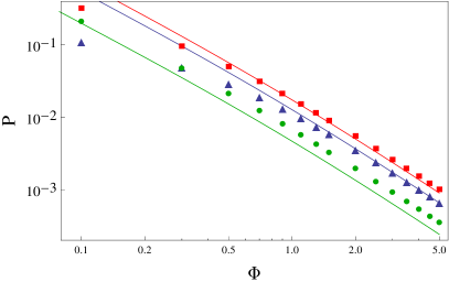
Figure 1: Fraction of destroyed axion miniclusters during their interactions with disk stars versus density perturbation $\Phi$ for the Galactic halo with the Navarro-Frenk-White density profile. The circles indicate the result of our calculation using Eq. (25), while the solid line indicates the approximate expression (38). The triangles indicate the result of our exact calculation using Eq. (32), while the corresponding solid line indicates the approximate expression (39). The total fraction of destroyed axion miniclusters is indicated by the squares, while the solid line passing through them indicates the sum of (38) and (39).

5 THE ISOTHERMAL DENSITY PROFILE

To ascertain how the result obtained depends on the Galactic halo model, let us perform calculations similar to the previous ones, but for the isothermal density profile of the Galactic halo

$$\rho_{\rm H}(r)=\frac{1}{4\pi}\frac{v_{\rm rot}^{2}}{Gr^{2}},$$ (40)

where $v_{\rm rot}=(GM_{\rm H}/R_{\rm H})^{1/2}$, $R_{\rm H}\simeq 200$ kpc, and $\rho(r)=0$ at $r>R_{\rm H}$. We choose $R_{c}=R_{\rm H}$; in this case, $U_{0}=v_{\rm rot}^{2}$ and the potential in dimensionless variables (11) is

$$\psi(r)=\log(\xi).$$ (41)

Using (9) for the profile (40) with the boundary at $r=R_{\rm H}$, we obtain

$$F(\varepsilon)=\frac{1}{2^{5/2}\pi^{3}e}\frac{v_{\rm rot}^{1/2}}{GM^{3/2}R_{\rm H}^{2}}\,F(\varepsilon),$$ (42)

where

$$f(\varepsilon)=\sqrt{2\pi}\,e^{-2\varepsilon+2}\,{\rm erf}\left[\sqrt{-2\varepsilon}\right]\!+\!\frac{e^{2}}{\sqrt{-\varepsilon}}.$$ (43)

Note that this distribution function does not reproduce the isothermal profile exactly.

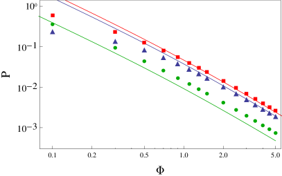
Figure 2: Fraction of destroyed axion miniclusters during their interactions with disk stars versus density perturbation $\Phi$ for the Galactic halo with the isothermal density profile. The circles indicate the result of our calculation using Eq. (25), while the solid line indicates the approximate expression (44). The triangles indicate the result of our exact calculation using Eq. (32), while the corresponding solid line indicates the approximate expression (45). The total fraction of destroyed axion miniclusters is indicated by the squares, while the solid line passing through them indicates the sum of (44) and (45).

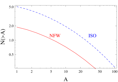
Figure 3: Detection rate of axion bursts (the number of bursts detected in 20 years of observations) with a density amplification larger than $A$. The solid curve indicates the result of our calculation in the case of the Navarro-Frenk-White profile for the sum of (38) and (39). The dashed curve indicates the result of our calculation in the case of the isothermal halo density profile for the sum of (44) and (45).

The fraction of clumps in the solar neighbourhood destroyed in their collisions with stars (25) found by numerically calculating all of the integrals in it is indicated by the dots in Fig. 2 for various values of $\Phi$. If the quantity in the exponent in (22) is much smaller than unity in absolute value, then

$$P\simeq\frac{1.3\times 10^{-2}}{\Phi^{3/2}(1+\Phi)^{1/2}}.$$ (44)

This result is indicated in Fig. 2 by the solid line.

The results of our calculation of the destruction by halo and bulge stars using Eq. (32) are indicated in Fig. 2 by the triangles. If the exponential in (29) can be expanded, then, as above, we approximately obtain

$$P^{(s)}=\frac{5.3\times 10^{-2}}{\Phi^{3/2}(1+\Phi)^{1/2}}.$$ (45)

This quantity and the total quantities for the isothermal density profile are shown in Fig. 2.

6 OBSERVATIONAL CONSEQUENCES

6.1 Detection of Streams in Axion Detectors

We calculate the expected detection rate of streams in ground-based detectors in the same way as was done in TinTkaZio16 . According to TinTkaZio16 (with the correction coefficient $3/2$ in Eq. (4.5) from TinTkaZio16 ), the frequency of stream-crossing events is

$$d\nu=\frac{3P_{\rm mc}(\Phi)[P(\Phi)+P^{(s)}(\Phi)]a(\Phi)}{2\tau(\Phi)A^{3}}dAd\Phi,$$ (46)

Here, $P_{\rm mc}(\Phi)$ is the distribution of axion miniclusters in perturbations $\Phi$, $a(\Phi)$ is the overdensity in the ministream with respect to the mean DM density in the Galactic halo in the solar neighbourhood $\rho_{\rm H}(r_{\odot})$ in the case where the minicluster is destroyed immediately after the Galactic disk formation (for more details, see TinTkaZio16 ), $A$ is the real overdensity in the ministream, and $\tau(\Phi)=2R/v$ is the passage time of the Earth through the ministream cross section. To obtain the detection rate of bursts $N(>A)=\nu(A)\Delta t$ with a density amplification larger than $A$ in an observation time $\Delta t$, it is necessary to integrate (46) over $\nu$ from ${\rm max}(A,a(\Phi))$ to $\bar{\rho}(\Phi)/\rho_{\rm H}(r_{\odot})$ and over all $\Phi$. The result of our calculations is indicated in Fig. 3 by the lower and upper lines for the Navarro-Frenk-White and isothermal density profiles, respectively.

Thus, we see that there is a dependence of the results on the Galactic halo model. For the Navarro-Frenk-White profile the destruction of clumps by the disk is approximately half as efficient as that for the singular isothermal halo. For the destruction by halo stars the isothermal profiles gives an almost a factor of 3 larger value.

6.2 On the Possibility of Detecting Streams by the LISA Detector

If a stream passes through the Solar system, then its gravitational field will act on gravitational-wave interferometers. The relative length of the interferometer arm $\Delta l/l$ will change under the tidal gravitational force from the stream. It is interesting to consider such an action on the planned LISA interferometer, which is expected to have a very high sensitivity, $\sim 2\times 10^{-18}$. The signals in the interferometer will be in the form of single pulses. The pulse structure in three directions will be strictly synchronized with the signals in the ground-based axion detectors. Therefore, based on the pattern of the pulses, it will be possible to prove almost unambiguously the passage of a stream and to ascertain its velocity direction and overall structure. The possibility of detecting compact objects with masses $10^{14}-10^{20}$ g using LISA was pointed out in LISAPBH , LISAAsteroid , LISADM , where primordial black holes, asteroids, or massive DM objects were considered as compact objects. In contrast to these papers, in our case, it is necessary to consider a noncompact mass distribution in the form of an elongated stream.

We model the stream by a straight thin thread of length $L=v_{\rm mc}t$, where $v_{\rm mc}$ is the internal velocity dispersion in the clump and $t$ is the time elapsed since the clump destruction. The gravitational field of the stream at distance $r$ from the axis is then

$$g=\frac{2GM}{rL}.$$ (47)

If $l\sim 5\times 10^{11}$ cm is the interferometer arm length (in the new eLISA project the arm length was reduced to $1\times 10^{11}$ cm), then the tidal acceleration is

$$\Delta g\sim\frac{2GM}{r^{2}L}l,$$ (48)

while the change of the arm length in the stream passage time $\Delta t\sim r/v_{\rm rel}$ is

$$\Delta l\sim\Delta g(\Delta t)^{2}/2,$$ (49)

where $v_{\rm rel}\sim 200$ km s^-1. The relative change of the arm is

$$\frac{\Delta l}{l}\sim\frac{GM}{v_{\rm rel}^{2}v_{\rm mc}t}\sim 3\times 10^{-19}$$ (50)

at $t\sim 5\times 10^{9}$ years. The quantity (50) does not depend on $r$ and is comparable to the LISA sensitivity. Slow streams with a lower $v_{\rm rel}$ will act on the detector more efficiently, but their number is also smaller. Axion streams will produce additional “noise” in space-borne detectors. The same expression for $\Delta l/l$ as (50) is also obtained if the passage of the interferometer arm inside a stream is considered.

To assess more accurately the prospects for the detection of axion streams by gravitational-wave interferometers, we will take into account the detector noise distribution. In our calculation we follow the method described in LISAPBH . Let $r_{\rm min}$ be the minimum distance from the axis of the passing stream to the center of the segment connecting the two interferometer mirrors. We will assume that during the passage the detector is always outside the stream. The tidal gravitational acceleration that the interferometer arm experiences is

$$a(t)=\frac{2GMl}{L[r_{\rm min}^{2}+(tv_{\rm rel})^{2}]},$$ (51)

while its Fourier spectrum is

$$a(f)=\int\limits_{-\infty}^{+\infty}dte^{2\pi ift}a(t)=\frac{2GMl}{Lv_{\rm rel}r_{\rm min}}e^{-2\pi r_{\rm min}f/v_{\rm rel}}.$$ (52)

If the detection is based on the optimal filtering method, then for the square of the signal-to-noise ratio we have

$$\rho^{2}_{\rm SN}=4\int\limits_{0}^{+\infty}df\frac{a^{2}(f)}{S^{2}(f)},$$ (53)

where for the LISA detector $S\simeq a_{0}\simeq 6\times 10^{-13}$ cm s^-2 Hz^-1/2. Assuming for the estimate that $S=a_{0}=const$, we obtain

$$\rho^{2}_{\rm SN}=\frac{4\pi G^{2}M^{2}l^{2}}{a_{0}^{2}L^{2}v_{\rm rel}r_{\rm min}^{3}}.$$ (54)

To detect a stream with a given $\rho_{\rm SN}$, it is necessary that the stream pass at a distance no larger than $r_{\rm min}$ from the detector. We numerically obtain

$$r_{\rm min}=6\times 10^{12}\left(\frac{l}{5\times 10^{12}\mbox{\leavevmode\nobreak\ cm}}\right)^{2/3}$$ (55)

$$\times \left(\frac{a_{0}}{6\times 10^{-13}\mbox{\leavevmode\nobreak\ cm\leavevmode\nobreak\ s${}^{-2}$\leavevmode\nobreak\ Hz${}^{-1/2}$}}\right)^{-2/3}\left(\frac{\Delta t}{5\times 10^{9}\mbox{\leavevmode\nobreak\ yars}}\right)^{-2/3}$$

$$\times \left(\frac{v_{\rm rel}}{200\mbox{\leavevmode\nobreak\ km\leavevmode\nobreak\ s${}^{-1}$}}\right)^{-2/3}\left(\frac{\rho_{\rm SN}}{0.05}\right)^{-2/3}\leavevmode\nobreak\ \mbox{cm},$$

With these normalization values the detection rate of streams will be

$${\rm Rate}=\pi r_{\rm min}^{2}v_{\rm rel}\frac{f_{\rm mc}\rho_{\rm DM}P}{M}\frac{v_{\rm mc}\Delta t}{R}\sim 0.1\mbox{\leavevmode\nobreak\ year${}^{-1}$},$$ (56)

where$f_{\rm mc}\sim 1$ is the fraction of DM in the form of axion miniclusters and $P\sim 0.02$ is the minicluster destruction probability calculated in previous sections.

Let us first consider the case with a single LISA-type detector. If we assume in (55) that the signal-to-noise ratio is $\rho_{\rm SN}\sim 5$, as is commonly assumed for a single detector, and choose $l=5\times 10^{11}$ cm, then (55) is smaller than the stream radius approximately by two orders of magnitude. The detection rate would be $\sim 10^{-5}$ yr^-1. Thus, next-generation detectors, in which the interferometer arm $l$ is larger than that in LISA by one and a half or two orders of magnitude and the noise $a_{0}$ is lower, are needed for the detection of streams with an acceptable rate. Allowance for the detector passage inside a stream and for the distribution in $v_{\rm rel}$, probably, will not change greatly the result. In the new eLISA project the detector noise at low frequencies is very large Amaetal12 ; at a characteristic frequency of $10^{-5}$ Hz we have $a_{0}\simeq 1.5\times 10^{-11}$ cm s^-2 Hz^-1/2. Therefore, in comparison with LISA, the detection rate of streams will be lower approximately by two more orders of magnitude. The dependence of the result on the distribution of clumps in velocities and directions is also interesting in the problem of the detection of clumps by gravitational-wave interferometers, but these questions are beyond the scope of this paper.

However, we may consider the detection of streams in two detectors, if there are two or more orbiting interferometers of the next (after LISA) generation, by the coincidence method and the characteristic signal shape. Suppose that the interferometer arm is an order of magnitude larger than was planned in LISA. In this case, a variant with $\rho_{\rm SN}<1$ is admissible, which was chosen in the normalization coefficients in (55) and (56). In this case, one might expect an acceptable detection rate from the viewpoint of real observations.

7 CONCLUSIONS

The particles being lost by a clump during its gravitational interactions with stars form a stream behind the clump being destroyed. In this way the bulk of the mass or the entire mass of the clump can pass into the stream. Since the area of the stream is larger than that of the clump by several orders of magnitude, the Earth’s passage through the stream is a much more probable event than its passage through the whole clump. Therefore, allowance for the streams is of great and, possibly, fundamental importance for the experiments aimed at directly detecting axion DM particles, as was shown in TinTkaZio16 .

In this paper we performed a calculation similar to that in TinTkaZio16 , but with allowance made for two additional effects. First, we took into account the fact that the orbits of clumps in the halo are noncircular and precess and that throughout its life history a clump could cross the Galactic disk at different distances from the center and could pass through halo regions with different number densities of stars. We considered two halo models, the Navarro-French-White profile and an isothermal sphere, and showed that the destruction in the second model is approximately a factor of two or three more efficient. Thus, the halo model affects noticeably the result. This influence is related to a different distribution of DM clumps in their orbital parameters.

The Navarro-Frenk-White profile was obtained in the numerical simulations of galaxies without including the baryonic component. The cooling of baryons and their settling to the halo center must lead to a deepening of the potential well and an additional increase of the DM density in the central halo region. Therefore, it is possible that the isothermal profile corresponds better to the real one, because in it the density concentration at the center is larger than that in the Navarro-Frenk-White halo.

Second, we took into account the destruction of clumps by Galactic halo and bulge stars. This effect increases the overall destruction efficiency. As is easy to show, the destruction of clumps during their pair interactions with one another is several orders of magnitude less efficient than that during the interactions of clumps with halo stars.

As a result, we obtained the distribution of the rate of stream-crossing events as a function of overdensity. For example, we found that at an overdensity $A>10$ one might expect 1-2 events in 20 years.

The prospects for the detection of streams from destroyed clumps with gravitational-wave interferometers look realistic only for detectors of the next (after LISA) generation or in the case of several LISA-type detectors and using a detection technique based on the coincidence method at a signal-to-noise ratio much less than unity in one detector.

We are grateful to D. Levkov and A. Panin for the useful discussions. This study was supported by the Russian Science Foundation (project no. 16-12-10494).

References

- (1) E. W. Kolb and I. I. Tkachev, Phys. Rev. D 50, 769 (1994); arXiv:astro-ph/9403011.
- (2) P. Tinyakov, I. Tkachev, K. Zioutas, JCAP 01, 035 (2016); arXiv:1512.02884 [astro-ph.CO].
- (3) V.S. Berezinsky, V.I. Dokuchaev and Yu.N.Eroshenko, JCAP 07, 011 (2007); arXiv:astro-ph/0612733.
- (4) V. Berezinsky, V. Dokuchaev, Yu. Eroshenko, Phys. Rev. D. 77, 083519 (2008); arXiv: 0712.3499 [astro-ph].
- (5) V. Berezinsky, V. Dokuchaev and Yu. Eroshenko, Phys. Rev. D. 73, 063504 (2006); arXiv:astro-ph/0511494.
- (6) A.V. Gurevich and K.P. Zybin, Sov. Phys. — JETP 67, 1 (1988); Sov. Phys. — JETP 67, 1957 (1988); Sov. Phys. — Usp. 165, 723 (1995).
- (7) O.Y. Gnedin and J.P. Ostriker, Astrophys. J. 513, 626 (1999).
- (8) J.E. Taylor and A. Babul, Astrophys. J. 559, 716 (2001).
- (9) J. Diemand, M. Kuhlen, P. Madau, Astrophys. J. 667, 859 (2007).
- (10) H.S. Zhao , J. Taylor, J. Silk and D. Hooper, arXiv:astro-ph/0502049v4.
- (11) T. Goerdt et al., Mon. Not. Roy. Astron. Soc. 375, 191 (2007).
- (12) M.D. Weinberg, Astron. J, 108, 1403 (1994).
- (13) P. Sikivie, I.I. Tkachev, Y. Wang, Phys. Rev. D. 56, 1863 (1997); arXiv:astro-ph/9609022.
- (14) A.S. Eddington, Mon. Not. Roy. Astron. Soc., 76, 572 (1916).
- (15) L.M. Widrow, Astrophys. J. Supp. 131, 39 (2000).
- (16) K. Kuijken, G. Gilmore, Mon. Not. Roy. Astron. Soc. 239, 605 (1989).
- (17) J.A.R.Caldwell, J.P. Ostriker, Astrophys. J. 251, 61 (1981).
- (18) L. S. Marochnik and A. A. Suchkov, The Galaxy (Nauka, Moscow, 1984) [in Russian].
- (19) B. Moore, J. Diemand, J. Stadel, T. Quinn; arXiv:astro-ph/0502213.
- (20) R. Launhardt, R. Zylka and P. G. Mezger, Astron. Astrophys. 384, 112 (2002).
- (21) N. Seto, A. Cooray , Phys. Rev. D 70, 063512 (2004).
- (22) P. Tricarico, Class. Quantum Grav. 26, 085003 (2009).
- (23) A.W. Adams, J.S. Bloom, arXiv:astro-ph/0405266.
- (24) P. Amaro-Seoane et al., Class. Quantum Grav. 29, 124016 (2012); arXiv:1202.0839 [gr-qc].