Lattice Boltzmann modeling of wall-bounded ternary fluid flows

Abstract

In this paper, a wetting boundary scheme used to describe the interactions among ternary fluids and solid is proposed in the framework of the lattice Boltzmann method. This scheme for three-phase fluids can preserve the reduction consistency property with the diphasic situation such that it could give physically relevant results. Combining this wetting boundary scheme and the lattice Boltzmann (LB) ternary fluid model based on the multicomponent phase-field theory, we simulated several ternary fluid flow problems involving solid substrate, including the spreading of binary drops on the substrate, the spreading of a compound drop on the substrate, and the shear of a compound liquid drop on the substrate. The numerical results are found to be good agreement with the analytical solutions or some available results. Finally, as an application, we use the LB model coupled with the present wetting boundary scheme to numerically investigate the impact of a compound drop on a solid circular cylinder. It is found that the dynamics of a compound drop can be remarkably influenced by the wettability of the solid surface and the dimensionless Weber number.

I Introduction

Multiphase flow systems involving ternary fluids and solid substrate have particular relevance and importance in the fields of environment and energy, such as enhanced oil recovery Maghzi , proton exchange membrane fuel cell hLi , droplet-based microfluidic chip Seemann , etc.. Within this context, the modeling of such flows is a challenging task since it involves the complex interactions among multiple fluids, and the formation of multiple contact angles on material substrate. Nonetheless, several researchers have made a great effort to develop efficient numerical approaches for simulating ternary fluid flows, which include the level set method Zhao ; Saye , volume of fluid method Bonhomme , smoothed particle hydrodynamic method Tofighi , and also the phase field method Garcke ; Boyer1 ; Kim ; Boyer2 ; Said ; Dong . Generally, these traditional numerical methods based on the macroscopic scale directly solve the incompressible Navier-Stokes equations coupled with a proper technique to track the phase interfaces. The methods have their own impressive versatility in simulating ternary fluid flows, while similar to two-phase scenario, some of them may have the limitation more or less, when they are readily applied to interfacial flows with large topological change Anderson . On the other hand, the dynamics of fluid interfaces physically can be recognized as a consequence of intermolecular interactions. In this regard, the numerical approaches based on the mesoscopic level may be more suitable to describe complex interfacial dynamics in ternary fluid systems with or without bounded wall.

The lattice Boltzmann (LB) method Guo1 , as a mesoscopic level method, has received considerable attention in the past two decades. It has some advantages over the traditional methods such as easy implementation of complex boundary and high efficiency of code parallelization. Particularly, due to its kinetic nature, the LB method can handle fluid-fluid and fluid-solid interactions directly, which can be regarded as its distinct advantage. From different physical perspectives, a wide range of multiphase, multicomponent models have been proposed in the framework of LB method, which can be commonly divided into four categories: color-gradient model Gunstensen , pseudo-potential model Shan , free-energy model Swift , and phase-field-based model He ; Lee ; Liang1 ; Liang2 ; Fakhari . Some improved variants based on these original multiphase models have also been proposed, and one can refer to the recent reviews Liu ; Li1 and references therein for the detailed expositions. Although a number of LB models have been developed for the two-phase case shown above, little attention in comparison has been paid to modelling multiphase systems involving ternary or more fluids in the LB community. Lamura et al. Lamura proposed a first lattice Boltzmann model for oil-water-amphiphile ternary systems, which is derived based on the minimisation of an appropriate free-energy functional. However, the model is only suitable to simulate ternary flows where an amphiphile phase is located at oil-water interface, and cannot be applied to arbitrary ternary flows. In addition, none distribution function is introduced to solely describe the species of amphiphile so that it has no orientational degree of freedom, which has been revised in the later developed free-energy model QunLi . Also from the viewpoint of the free-energy functional, Semprebon et al. Semprebon recently proposed a LB model for ternary fluids that can adjust independently the surface tensions among fluids and the contact angles on the substrate. Chen et al. Chen ; Nekovee developed another lattice Boltzmann model for simulating oil-water-amphiphile ternary flows, which can be regarded as an extension of the original pseudo-potential model Shan by considering interactions among three fluid components. The generalization of the color-gradient model to multiple immiscible continuum fluids was attributed to Halliday et al. Halliday1 ; Halliday2 , who introduced a color gradient for each of fluid-fluid interfaces in the color model, while their models are limited to fluids with a very small density difference. To remove this limitation, Leclaire et al. Leclaire developed a LB model based on the improved color-gradient model, where three subcollision operators are also applied. As a result, their model is able to deal with the multi-componet flows with moderate density ratios. Recently, Liang et al. Liang3 presented an alternative LB ternary model based on the Cahn-Hilliard phase-field theory, which provides a firm physical foundation on the dynamics of the interfaces among three fluids. Actually, the phase-field based LB models for multiphase flows have showed great potential in the study of complex interfacial flows Liang1 ; Liang4 .

As reviewed above, most of the aforementioned LB models only focus on ternary fluid flows in the absence of bounded solid wall, with a recent exception Semprebon . Oftentimes, ternary fluids are encountered with solid substrate in applications mentioned above, and its wettability plays a vital role in fluid interfacial dynamics. Therefore, how to describe the interactions among fluids and solid is a very cruial problem. Our main focus in this paper will be on the phase-field-based LB ternary model Liang3 . As a continuous work, a suitable wetting boundary scheme that describe the interations among fluids and solid is proposed in the framework of the LB method. One distinct feature of the scheme lies in the reduction consistency property which matches that of the LB ternary model Liang3 . Besides, multiple equilibrium contact angles can be given explicitly in the boundary condition formulation. The rest of the paper is organized as follows. In Sec. II, we firstly gives a brief introduction of the LB ternary method, and then present a novel wetting boundary scheme for ternary fluids. Numerical experiments to validate the present scheme can be found in Sec. III, where a compound drop impact on the solid cylinder is also studied. At last, we made a summary in Sec. IV.

II LB method for wall-boundary ternary fluid flows

II.1 LB method for ternary fluid flows

In this subsection, we give a brief introduction on the LB method for ternary fluid flows, and a detailed description can be found in Ref. Liang3 . The LB method consists of three LB equations, two of which is used to capture the interfaces among three-component fluids and the other is used to derive the fluid velocity and pressure. The LB evolution equations with the BGK collision operator can be written as Liang3 ; Guo2

$${f^{i}_{k}}({\bf{x}}+{{\bf{e}}_{k}}{\delta_{t}},t+{\delta_{t}})-{f^{i}_{k}}({\bf{x}},t)=-\frac{1}{\tau_{i}}\left[{{f^{i}_{k}}({\bf{x}},t)-f_{k}^{i,eq}({\bf{x}},t)}\right]+{\delta_{t}}{F^{i}_{k}}({\bf{x}},t),$$ (1a)

$${g}_{k}({\bf{x}}+{{\bf{e}}_{k}}{\delta_{t}},t+{\delta_{t}})-{g}_{k}({\bf{x}},t)=-\frac{1}{\tau_{g}}[{{g}_{k}({\bf{x}},t)-g_{k}^{eq}({\bf{x}},t)}]+{\delta_{t}}G_{k}({\bf{x}},t),$$ (1b)

where the superscript $i$ taking $1$ or $2$ represents the $i$-th phase, $f^{i}_{k}({\bf{x}},t)$ and $g_{k}({\bf{x}},t)$ are the distribution functions, $f_{k}^{i,eq}({\bf{x}},t)$ and $g_{k}^{eq}({\bf{x}},t)$ are the corresponding equilibrium functions, $\tau_{i}$ and ${\tau_{g}}$ are the non-dimensional relaxation times, $\delta_{t}$ is the time step. To recover the macroscopic equations exactly, the equilibrium distribution functions $f_{k}^{i,eq}$ and $g_{k}^{eq}$ are delicately designed as Shi ; Chai ; Liang1

$$f_{k}^{i,eq}=\left\{\begin{array}[]{ll}c_{i}+({\omega_{k}}-1)\eta{\mu_{i}},&\textrm{ $k=0$}\\ {\omega_{k}}\eta{\mu_{i}}+{\omega_{k}}c_{i}{{{\textbf{e}_{k}}\cdot{\bf{u}}}\over{c_{s}^{2}}},&\textrm{ $k\neq 0$},\end{array}\right.$$ (2a)

$$g_{k}^{eq}=\left\{\begin{array}[]{ll}{p\over{c_{s}^{2}}}({\omega_{k}}-1)+\rho{s_{k}}({\bf{u}}),&\textrm{ $k=0$},\\ {p\over{c_{s}^{2}}}{\omega_{k}}+\rho{s_{k}}({\bf{u}}),&\textrm{ $k\neq 0$},\\ \end{array}\right.$$ (2b)

where $c_{i}$ is the order parameter that represents the volume fraction of $i$-th phase within the mixture. In the phase-field models, one should use three order parameters marked by $c_{1}$, $c_{2}$, and $c_{3}$ to describe a ternary system, and they are linked through the constraint Boyer1 ; Kim ; Boyer2 ,

$$c_{1}+c_{2}+c_{3}=1.$$ (3)

In Eqs. (2a) and (2b), $\omega_{k}$ is the weighting coefficient, $\textbf{e}_{k}$ is the discrete velocity, $c_{s}$ is the sound speed, $\eta$ is an adjustable parameter, and ${s_{k}}({\bf{u}})$ is defined by Liang1 ; Liang3

$${s_{k}}({\bf{u}})={\omega_{k}}\left[{{{{{\bf{e}}_{k}}\cdot{\bf{u}}}\over{c_{s}^{2}}}+{{{{({{\bf{e}}_{k}}\cdot{\bf{u}})}^{2}}}\over{2c_{s}^{4}}}-{{{\bf{u}}\cdot{\bf{u}}}\over{2c_{s}^{2}}}}\right].$$ (4)

${\mu_{i}}$ in Eq. (2a) is the chemical potential, which depends on the variational derivative of the bulk free energy with respect to the order parameters in the ternary phase-field models. Up to now, several researchers have conducted theoretical analyses on the form of the bulk free energy Garcke ; Boyer1 ; Kim ; Boyer2 ; Said . Here the one reported in Ref. Boyer1 ; Boyer2 is used since it can be well-posed and also satisfies the algebraically and dynamically consistency conditions. Then, the bulk free energy takes the following form Boyer1 ; Boyer2 ,

$$F(c_{1},c_{2},c_{3})=\frac{\lambda_{1}}{2}{c_{1}^{2}}(1-c_{1})^{2}+\frac{\lambda_{2}}{2}{c_{2}^{2}}(1-c_{2})^{2}+\frac{\lambda_{3}}{2}{c_{3}^{2}}(1-c_{3})^{2}+{\lambda}{c_{1}^{2}}{c_{2}^{2}}{c_{3}^{2}},$$ (5)

where ${\lambda}$ is a non-negative parameter, and the chemical potential ${\mu_{i}}$ can be derived by Boyer1 ; Boyer2

$$\mu_{i}=\frac{4\lambda_{T}}{D}{\sum\limits_{j\neq{i}}}\left[\frac{1}{\lambda_{j}}\left(\frac{\partial F}{\partial{c_{i}}}-\frac{\partial F}{\partial{c_{j}}}\right)\right]-\frac{3}{4}{D}{\lambda_{i}}\nabla^{2}{c_{i}},$$ (6)

where the parameters ${\lambda_{i}}$ $(i=1,2,3)$ are related to the surface tensions,

$${\lambda_{1}}=\sigma_{12}+\sigma_{13}-\sigma_{23}$$

$${\lambda_{2}}=\sigma_{12}+\sigma_{23}-\sigma_{13}$$

$${\lambda_{3}}=\sigma_{13}+\sigma_{23}-\sigma_{12},$$ (7)

where $\sigma_{23}$, $\sigma_{23}$ and $\sigma_{23}$ represent the surface tension between two fluids of a three-phase system. When ${\lambda_{i}}$ $(i=1,2,3)$ are all positive and further satisfy ${\lambda_{i}}>0.5{\lambda_{T}}$ [see Eq. (9)], the bulk free energy with ${\lambda}=0$ can give physically relevant results Boyer1 ; Liang3 , which will be adopted in our numerical simulations. In this case, one can simplify Eq. (6) as

$$\mu_{i}=\frac{12}{D}\left[{\lambda_{i}}{c_{i}}(1-c_{i})(1-2c_{i})-2{\lambda_{T}}{c_{1}}{c_{2}}(1-c_{1}-c_{2})\right]-\frac{3}{4}{D}{\lambda_{i}}\nabla^{2}{c_{i}},$$ (8)

where $D$ is the interface thickness, and ${\lambda_{T}}$ is defined by

$$\frac{3}{\lambda_{T}}={\sum\limits_{i=1}^{3}{\frac{1}{\lambda_{i}}}}.$$ (9)

In the present work, the D2Q9 lattice model is used without loss of generality, where the weighting coefficients $\omega_{k}$ are given by $\omega_{0}=4/9$, $\omega_{1-4}=1/9$, $\omega_{5-8}=1/36$, and the discrete velocities $\textbf{e}_{k}$ are Guo2

$$\mathbf{e}_{k}=\left\{\begin{array}[]{ll}(0,0)c,&\textrm{ $k=0$},\\ (\cos[(k-1)\pi/2],\sin[(k-1)\pi/2])c,&\textrm{ $k=1-4$},\\ \sqrt{2}(\cos[(k-5)\pi/2+\pi/4],\sin[(k-5)\pi/2+\pi/4])c,&\textrm{ $k=5-8$},\end{array}\right.$$ (10)

where $c=\delta_{x}$/$\delta_{t}$ is the lattice speed with $\delta_{x}$ representing the grid spacing, $c_{s}=c/\sqrt{3}$. For simplicity, we set the grid space and time increment as the length and time units, i.e., $\delta_{x}=\delta_{t}=1$.

To derive the correct governing equations, the proper source term ${F^{i}_{k}}$ and forcing term ${{G}_{k}}$ should be incorporated in the LB evolution equation, which can be defined as Liang1 ; Liang3

$${{F}^{i}_{k}}=(1-\frac{1}{2\tau_{i}}){{{\omega_{k}}{{\bf{e}}_{k}}\cdot{\partial_{t}}c_{i}{\bf{u}}}\over{c_{s}^{2}}},~{}~{}~{}i=1,~{}2,$$ (11a)

$${{G}_{k}}=(1-\frac{1}{2\tau_{g}}){({{\bf{e}}_{k}}-{\bf{u}})}\cdot\left[{{s_{k}}({\bf{u}})\nabla{\rho}+({s_{k}}({\bf{u}})+\omega_{k}){\frac{({{\bf{F}}_{s}}+{\bf{G}})}{c_{s}^{2}}}}\right]+\frac{{\omega_{k}}{\mathbf{e}_{k}}\cdot{\mathbf{F}_{a}}}{c_{s}^{2}},$$ (11b)

where ${\bf{G}}$ is the body force, ${{\bf{F}}_{a}}$ is the additional interfacial force, ${\bf{F}}_{s}$ is the surface tension force, which can take several different forms. Here we take the potential form $\mathbf{F}_{s}=\sum\limits_{i=1}^{3}{\mu_{i}}\nabla{c_{i}}$, as widely used in the ternary phase-field models Boyer1 ; Boyer2 ; Liang3 . ${{\bf{F}}_{a}}$ introduced in Eq. (11b) is used to recover the correct momentum equation, which can be defined as Liang3

$${{\bf{F}}_{a}}=\mathbf{u}\sum_{i=1}^{2}(\rho_{i}-\rho_{3}){M_{i}}\nabla^{2}\mu_{i},$$ (12)

where $M_{i}=M_{0}/\lambda_{i}$ is the diffusion coefficient in the interfacial governing equation, and $M_{0}$ is a positive parameter. In the LB algorithm, the macroscopic quantities, $c_{i}$, ${\bf{u}}$ and $p$ are evaluated as Liang3 ,

$$c_{i}=\sum\limits_{k}{{f^{i}_{k}}},~{}~{}~{}i=1,~{}2,$$ (13a)

$${\bf{u}}=\frac{1}{\rho}\left[{{\sum\limits_{k}{{{\bf{e}}_{k}}{g_{k}}}+0.5{\delta_{t}}({{\bf{F}}_{s}}+{\bf{G}})}}\right],$$ (13b)

$$p={{c_{s}^{2}}\over{(1-{\omega_{0}})}}\left[{\sum\limits_{k\neq 0}{{g_{k}}}+{{{\delta_{t}}}\over 2}{\bf{u}}\cdot\nabla\rho+\rho{s_{0}}(\textbf{u})}\right],$$ (13c)

and the order parameter $c_{3}$ can be derived from the conservation (3). For the sake of simplicity, we assume that the fluid density and viscosity are the linear interpolations of three order parameters Kim

$$\rho={c_{1}}{\rho_{1}}+{c_{2}}{\rho_{2}}+(1-{c_{1}}-{c_{2}}){\rho_{3}},$$ (14)

$$\nu={c_{1}}{\nu_{1}}+{c_{2}}{\nu_{2}}+(1-{c_{1}}-{c_{2}}){\nu_{3}},$$ (15)

where $\rho_{i}$ and $\nu_{i}$ $(i=1,2,3)$ are the density and viscosity of the $i$-th phase. Through Chapman-Enskog analysis Liang1 ; Liang3 , it is shown that the multi-component Cahn-Hilliard equations

$${{\partial{c_{i}}}\over{\partial t}}+\nabla\cdot{c_{i}}{\bf{u}}=\nabla\cdot\left({M_{i}}\nabla{\mu_{i}}\right),$$ (16)

and the incompressible Navier-Stokes equations

$$\nabla\cdot{\bf{u}}=0,$$ (17a)

$$\rho({{\partial{\bf{u}}}\over{\partial t}}+{\bf{u}}\cdot\nabla{\bf{u}})=-\nabla p+\nabla\cdot\left[{\nu\rho(\nabla{\bf{u}}+\nabla{{\bf{u}}^{T}})}\right]+{{\bf{F}}_{s}}+{\bf{G}},$$ (17b)

can be derived from the present model. Additionally, one can derive the expressions of the mobility $M_{i}$ and the kinematic viscosity $\nu$ as Liang1 ; Liang3 ,

$${M_{i}}=\eta c_{s}^{2}(\tau_{i}-0.5)\delta t,~{}i=1,~{}2,$$ (18a)

$$\nu=c_{s}^{2}(\tau_{g}-0.5){\delta_{t}}.$$ (18b)

For the numerical computations, the time derivative in Eq. (11a) and the spatial gradients in Eq. (11b) should be discretized with suitable difference schemes. In this work, the explicit Euler scheme Shi ,

$$\partial_{t}\chi({\bf{x}},t)=\frac{\chi({\bf{x}},t)-\chi({\bf{x}},t-\delta_{t})}{\delta_{t}},$$ (19)

is applied for calculating the time derivative and the second-order isotropic central schemes Liang1 ,

$$\nabla\chi({\bf{x}},t)=\sum\limits_{k\neq 0}{\frac{\omega_{k}\textbf{e}_{k}\chi({\bf{x}}+{{\bf{e}}_{k}}{\delta_{t}},t)}{c_{s}^{2}\delta_{t}}}$$ (20a)

$$\nabla^{2}\chi({\bf{x}},t)=\sum\limits_{k\neq 0}{\frac{2\omega_{k}[\chi({\bf{x}}+{{\bf{e}}_{k}}{\delta_{t}},t)-\chi({\bf{x}},t)]}{c_{s}^{2}\delta_{t}^{2}}},$$ (20b)

are adopted to compute the gradient operators, where $\chi$ represents an arbitrary variable.

II.2 Wetting boundary condition for ternary fluid flows

The lattice Boltzmann model for ternary fluid flows is developed based on the ternary phase-field theory Boyer1 ; Boyer2 , where the wall wetting effect has not been considered. In order to simulate three-phase flows in contact with solid wall, a suitable wetting boundary condition should be established to describe the interactions among fluids and solid, and its scheme in the framework of the LB method should also be given. The wetting boundary condition for ternary fluid flows can be constructed by considering an additional wall free energy. Denoting the flow domain by $\Omega$ and the solid boundary by ${\partial\Omega}$, the total free energy of a three-phase system can be expressed as Yshi

$$\Psi_{tot}=\int_{\Omega}\left[\frac{12}{D}F(c_{1},c_{2},c_{3})+\sum\limits_{i=1}^{3}{\frac{3}{8}D{\lambda_{i}}|\nabla{c_{i}}|^{2}}\right]d\Omega+\int_{\partial\Omega}{\psi_{s}}(c_{1},c_{2},c_{3})ds,$$ (21)

where $F(c_{1},c_{2},c_{3})$ is the bulk free energy, ${\psi_{s}}(c_{1},c_{2},c_{3})$ is the free energy density on the solid boundary. Boyer et al. Boyer1 ; Boyer2 have showed that the model without including the boundary effect is algebraically consistent with the diphasic system only if the bulk free energy $F(c_{1},c_{2},c_{3})$ and the physical parameters ${\lambda_{i}}$ are given by Eqs. (5) and (7), respectively. The expression of the free energy density ${\psi_{s}}(c_{1},c_{2},c_{3})$ is also determined based on the reduction consistency condition. For the convenience of discussion, we first give a brief overview of the phase-field model with the wall effect for two-phase flows. In a two-phase system, the total free energy has the following form Lee ; Zhang ,

$$\Psi=\int_{\Omega}\left[\frac{12}{D}{\sigma}c^{2}(1-c)^{2}+\frac{3}{4}{\sigma}D|\nabla c|^{2}\right]d\Omega+\int_{\partial\Omega}{\psi_{s}}(c)ds,$$ (22)

where $c$ is the order parameter with the values of $0$ and $1$ in the bulk phase regions, and varies continuously across the interfacial zone with the thickness $D$, $\sigma$ is the surface tension between two fluids, ${\psi_{s}}(c)$ is the free energy density on the solid wall given by Lee ; Zhang

$${\psi_{s}}(c)=\sigma_{w1}+(\sigma_{w2}-\sigma_{w1})(3c^{2}-2c^{3}),$$ (23)

where $\sigma_{w1}$ and $\sigma_{w2}$ denote the fluid-wall surface tensions. Minimizing the total free energy, one can derive the two-phase wetting boundary condition,

$$\frac{3}{2}\sigma D\mathbf{n}\cdot\nabla{c}+\frac{\partial{\psi_{s}}(c)}{\partial c}=0,$$ (24)

where $\mathbf{n}$ is the unit normal vector with the direction from the fluid toward the solid. Substituting Eq. (23) into the above relation, one can rewrite Eq. (24) as

$$\frac{3}{2}\sigma D\mathbf{n}\cdot\nabla{c}+6(\sigma_{w2}-\sigma_{w1})(c-c^{2})=0,$$ (25)

For the two-phase fluids on the chemically homogeneous wall, the wettability of the wall can be evaluated by the contact angle ($\theta$), which is determined by the Young’s equation associated with the surface tensions at the fluid-solid junction Said ; Dong , $\cos{\theta}=(\sigma_{w1}-\sigma_{w2})/\sigma$. Then, Eq. (25) can be recast as

$$\mathbf{n}\cdot\nabla{c}=\frac{4\cos\theta}{D}(c-c^{2}).$$ (26)

To be consistent with the diphasic case, the free energy density ${\psi_{s}}(c_{1},c_{2},c_{3})$ in a three-phase system can be chosen as,

$${\psi_{s}}(c_{1},c_{2},c_{3})=\sigma_{w1}(3c_{1}^{2}-2c_{1}^{3})+\sigma_{w2}(3c_{2}^{2}-2c_{2}^{3})+\sigma_{w3}(3c_{3}^{2}-2c_{3}^{3}),$$ (27)

where $\sigma_{wi}$ $(i=1,2,3)$ represents the surface tension between the solid wall and the $i$-th fluid. One can easily find that Eq. (27) can reduce to the two phase formulation (23), when setting $c_{1}=1-c$, $c_{2}=c$, $c_{3}=0$. In the following, we use the symbol ${\psi_{s}}$ to mark ${\psi_{s}}(c_{1},c_{2},c_{3})$ for simplicity. The wetting boundary condition for ternary fluid flows can be derived by minimizing the total free energy (21). However, in order to satisfy the conservation (3), an additional term $\Lambda_{i}$ as a function of the order parameters is also introduced. Then, the wetting boundary condition can be expressed as,

$$\frac{3}{4}{\lambda_{i}}D\mathbf{n}\cdot\nabla{c_{i}}+\frac{\partial{\psi_{s}}}{\partial c_{i}}+\Lambda_{i}=0,~{}i=1,2,3,$$ (28)

which can be further written as

$$\frac{3}{4}{\lambda_{i}}D\mathbf{n}\cdot\nabla{c_{i}}+g_{i}=0,~{}i=1,2,3,$$ (29)

where $g_{i}$ is defined by $g_{i}=\frac{\partial{\psi_{s}}}{\partial c_{i}}+\Lambda_{i}$. Now we give details on how to derive the expression of $g_{i}$. Summing Eq. (29) over $i$ and denoting $S=c_{1}+c_{2}+c_{3}$, one can easily obtain the following equation,

$$\frac{3}{4}D\mathbf{n}\cdot\nabla{S}+\sum_{i=1}^{3}\frac{g_{i}}{{\lambda_{i}}}=0.$$ (30)

Because of the conservation (3), $S=1$ should be the solution of Eq. (30), and we can then derive

$$\sum_{i=1}^{3}\frac{g_{i}}{{\lambda_{i}}}=0.$$ (31)

As pointed in Refs. Boyer1 ; Boyer2 , to be algebraically consistent with the diphasic system, the ternary model should preserve the property that the $i$-th phase does not appear during the time evolution of the system if it is absent at initial time. To satisfy this property, from Eq. (31) one can obtain the following relations,

$${g_{i}}|_{(c_{i}=0)}=0,$$ (32)

for $i$=1, 2 and 3. Supposing ${\Lambda_{i}}$ being the linear combination of $\frac{\partial{\psi_{s}}}{\partial c_{j}}$ Yshi , ${g_{i}}$ can then be written in the vector form,

$${\mathbf{g}}=\mathbf{A}\cdot\frac{\partial\psi_{s}}{\partial{\mathbf{c}}},$$ (33)

where $\mathbf{g}=(g_{1},g_{2},g_{3})^{T}$, $\mathbf{A}$ is a $3\times 3$ matrix, and $\frac{\partial\psi_{s}}{\partial{\mathbf{c}}}=(\frac{\partial\psi_{s}}{\partial{c_{1}}},\frac{\partial\psi_{s}}{\partial{c_{2}}},\frac{\partial\psi_{s}}{\partial{c_{3}}})^{T}$. From the above constraint conditions, we can choose the matrix $\mathbf{A}$ as

$$\mathbf{A}=\frac{1}{2}\left[\begin{array}[]{ccccccc}\frac{\lambda_{1}}{\sigma_{12}}\frac{c_{2}}{1-c_{1}}+\frac{\lambda_{1}}{\sigma_{13}}\frac{c_{3}}{1-c_{1}}&-\frac{\lambda_{1}}{\sigma_{12}}\frac{c_{1}}{1-c_{2}}&-\frac{\lambda_{1}}{\sigma_{13}}\frac{c_{1}}{1-c_{3}}\\ -\frac{\lambda_{2}}{\sigma_{12}}\frac{c_{2}}{1-c_{1}}&\frac{\lambda_{2}}{\sigma_{12}}\frac{c_{1}}{1-c_{2}}+\frac{\lambda_{2}}{\sigma_{23}}\frac{c_{3}}{1-c_{2}}&-\frac{\lambda_{2}}{\sigma_{23}}\frac{c_{2}}{1-c_{3}}\\ -\frac{\lambda_{3}}{\sigma_{13}}\frac{c_{3}}{1-c_{1}}&-\frac{\lambda_{3}}{\sigma_{23}}\frac{c_{3}}{1-c_{2}}&\frac{\lambda_{3}}{\sigma_{13}}\frac{c_{1}}{1-c_{3}}+\frac{\lambda_{3}}{\sigma_{23}}\frac{c_{2}}{1-c_{3}}\end{array}\right],$$ (34)

and $g_{i}$ can then be derived as

$$g_{1}=\frac{3\lambda_{1}}{\sigma_{13}}(\sigma_{w1}-\sigma_{w3}){c_{1}}{c_{3}}+\frac{3\lambda_{1}}{\sigma_{12}}(\sigma_{w1}-\sigma_{w2}){c_{1}}{c_{2}},$$

$$g_{2}=\frac{3\lambda_{2}}{\sigma_{12}}(\sigma_{w2}-\sigma_{w1}){c_{1}}{c_{2}}+\frac{3\lambda_{2}}{\sigma_{23}}(\sigma_{w2}-\sigma_{w3}){c_{2}}{c_{3}},$$

$$g_{3}=\frac{3\lambda_{3}}{\sigma_{23}}(\sigma_{w3}-\sigma_{w2}){c_{2}}{c_{3}}+\frac{3\lambda_{3}}{\sigma_{13}}(\sigma_{w3}-\sigma_{w1}){c_{1}}{c_{3}}.$$ (35)

With some algebraic manipulations, one can easily find that Eqs. (31) and (32) can be satisfied. Additionally, the wetting boundary condition for three-phase flows given in Eqs. (29) and (35) can exactly degenerate to the two-phase case when one component vanishes. For instance, when the $3$-th phase is not present in the system, i.e., $c_{3}=0$, and $c_{1}+c_{2}=1$, $g_{i}$ can be simplified as

$$g_{1}=\frac{3\lambda_{1}}{\sigma_{12}}(\sigma_{w1}-\sigma_{w2}){c_{1}}{c_{2}},~{}~{}g_{2}=\frac{3\lambda_{2}}{\sigma_{12}}(\sigma_{w2}-\sigma_{w1}){c_{1}}{c_{2}},~{}~{}g_{3}=0,$$ (36)

and the boundary scheme is

$$\frac{3}{2}\sigma_{12}D\mathbf{n}\cdot\nabla{c_{2}}+3(\sigma_{w2}-\sigma_{w1}){c_{1}}{c_{2}}=0,$$ (37)

which is consistent with the two-phase formulation (25). Considering the ternary fluids in contact with the chemically homogeneous substrate, we could describe the wettability of the substrate in terms of three static contact angles, which satisfy the Young’s relation Ding2 ; Dong ,

$$\cos{\theta_{ij}}=\frac{\sigma_{wj}-\sigma_{wi}}{\sigma_{ij}},~{}~{}1\leq i<j\leq 3,$$ (38)

where $\theta_{ij}$ is the static contact angle between the wall and the interface formed by fluids $i$ and $j$. The values of $\theta_{12}$, $\theta_{13}$, and $\theta_{23}$ cannot be arbitrarily chosen, and should satisfy the following constraint,

$$\sigma_{12}\cos{\theta_{12}}-\sigma_{13}\cos{\theta_{13}}+\sigma_{23}\cos{\theta_{23}}=0.$$ (39)

With the substitution of Eq. (35) into Eq. (29) and using the relation (38), we can ultimately derive the wetting boundary condition for three-phase flows,

$$\mathbf{n}\cdot\nabla{c_{1}}=\frac{4}{D}(\cos{\theta_{13}}{c_{1}}{c_{3}}+\cos{\theta_{12}}{c_{1}}{c_{2}}),$$

$$\mathbf{n}\cdot\nabla{c_{2}}=\frac{4}{D}(-\cos{\theta_{12}}{c_{1}}{c_{2}}+\cos{\theta_{23}}{c_{2}}{c_{3}}),$$

$$\mathbf{n}\cdot\nabla{c_{3}}=\frac{4}{D}(-\cos{\theta_{23}}{c_{2}}{c_{3}}-\cos{\theta_{13}}{c_{1}}{c_{3}}).$$ (40)

We now introduce how the three-phase wetting boundary condition is implemented in the framework of the LB method. The wetting boundary condition given in Eq. (40) is valid at equilibrium, and thus is only imposed for the term related to free energy, i.e., $\nabla^{2}c_{i}$ in Eq. (8). Once the $\nabla^{2}c_{i}$ is prescribed, $\mu_{i}$ in Eq. (8) is treat as a scalar Lee . The $\nabla^{2}c_{i}$ can be computed by Eq. (20b). While for the fluid node next to the solid wall, the computation of $\nabla^{2}c_{i}$ should be specifically treated by imposing it the wetting boundary formulation (40), and the details are given as follows. As depicted in Fig. 1, $\mathbf{x}_{f}$ is the fluid node next to the boundary layer, $\mathbf{x}_{w}$ is the solid boundary node with one half lattice length from $\mathbf{x}_{f}$, and $\mathbf{x}_{f}+\mathbf{e}_{k}\delta_{t}$ is the ghost node. To determine the value of $\nabla^{2}c_{i}$ at the $\mathbf{x}_{f}$, the macroscopic information at the ghost node $\mathbf{x}_{f}+\mathbf{e}_{k}\delta_{t}$ should be specified. After the central discretization for the left-hand side of Eq. (40), we then get

$$\frac{{c_{{1},\mathbf{x}_{f}+\mathbf{e}_{k}\delta_{t}}}-{c_{{1},\mathbf{x}_{f}}}}{\delta_{x}}=\frac{4}{D}(\cos{\theta_{13}}{c_{1,\mathbf{x}_{w}}}{c_{3,\mathbf{x}_{w}}}+\cos{\theta_{12}}{c_{1,\mathbf{x}_{w}}}{c_{2,\mathbf{x}_{w}}}),$$

$$\frac{{c_{{2},\mathbf{x}_{f}+\mathbf{e}_{k}\delta_{t}}}-{c_{{2},\mathbf{x}_{f}}}}{\delta_{x}}=\frac{4}{D}(-\cos{\theta_{12}}{c_{1,\mathbf{x}_{w}}}{c_{2,\mathbf{x}_{w}}}+\cos{\theta_{23}}{c_{2,\mathbf{x}_{w}}}{c_{3,\mathbf{x}_{w}}}),$$

$$\frac{{c_{{3},\mathbf{x}_{f}+\mathbf{e}_{k}\delta_{t}}}-{c_{{3},\mathbf{x}_{f}}}}{\delta_{x}}=\frac{4}{D}(-\cos{\theta_{23}}{c_{2,\mathbf{x}_{w}}}{c_{3,\mathbf{x}_{w}}}-\cos{\theta_{13}}{c_{1,\mathbf{x}_{w}}}{c_{3,\mathbf{x}_{w}}}).$$ (41)

As shown above, the variables ${c_{{i},\mathbf{x}_{w}}}$ $(i=1,2,3)$ that represent the distributions of the phase fields at the solid wall are unknown. Here we use the interpolation ${c_{{i},\mathbf{x}_{w}}}={c_{{i},\mathbf{x}_{f}}}$ to estimate their values, which is commonly used in the boundary scheme of the LB method Guo3 . As a result, we ultimately derive the distributions of the order parameters at the ghost node,

$${c_{{1},\mathbf{x}_{f}+\mathbf{e}_{k}\delta_{t}}}={c_{{1},\mathbf{x}_{f}}}+\frac{4\delta_{x}}{D}(\cos{\theta_{13}}{{c}_{1,\mathbf{x}_{f}}}{{c}_{3,\mathbf{x}_{f}}}+\cos{\theta_{12}}{{c}_{1,\mathbf{x}_{f}}}{{c}_{2,\mathbf{x}_{f}}}),$$

$${c_{{2},\mathbf{x}_{f}+\mathbf{e}_{k}\delta_{t}}}={c_{{2},\mathbf{x}_{f}}}+\frac{4\delta_{x}}{D}(-\cos{\theta_{12}}{{c}_{1,\mathbf{x}_{f}}}{{c}_{2,\mathbf{x}_{f}}}+\cos{\theta_{23}}{{c}_{2,\mathbf{x}_{f}}}{{c}_{3,\mathbf{x}_{f}}}),$$

$${c_{{3},\mathbf{x}_{f}+\mathbf{e}_{k}\delta_{t}}}={c_{{3},\mathbf{x}_{f}}}+\frac{4\delta_{x}}{D}(-\cos{\theta_{23}}{{c}_{2,\mathbf{x}_{f}}}{{c}_{3,\mathbf{x}_{f}}}-\cos{\theta_{13}}{{c}_{1,\mathbf{x}_{f}}}{{c}_{3,\mathbf{x}_{f}}}).$$ (42)

From Eq. (42), the values of the order parameters at the ghost node has been determined, and then $\nabla^{2}c_{i}$ at the fluid nodes neighboring to solid wall can be computed by Eq. (20b).

In addition to the computation of $\nabla^{2}c_{i}$, the space gradients $\nabla c_{i}$, $\nabla{\rho}$ and $\nabla^{2}\mu_{i}$ at the fluid node $\mathbf{x}_{f}$ should also be given in the LB algorithm. The evaluation of these gradients using Eqs. (20a) and (20b) require the unknown information at the ghost node $(\mathbf{x}_{f}+\mathbf{e}_{k}\delta_{t})$, which can be determined based on the symmetric rule with respect to the solid wall Liang2 ,

$$c_{i}(\mathbf{x}_{f}+\mathbf{e}_{k}\delta_{t})=c_{i}(\mathbf{x}_{f}),$$

$$\rho(\mathbf{x}_{f}+\mathbf{e}_{k}\delta_{t})=\rho(\mathbf{x}_{f}),$$

$$\mu_{i}(\mathbf{x}_{f}+\mathbf{e}_{k}\delta_{t})=\mu_{i}(\mathbf{x}_{f}).$$ (43)

The scheme in Eq. (43) used here satisfies no flux condition, and also can avoid unphysical mass and momentum transfer through the solid boundary. The boundary conditions for the distribution functions should also be specified in the implementation of the LB method. In this work, we apply the half-way bounce back boundary scheme for dealing with the solid wall, which is realized by setting the unknown distribution functions to be the ones in the opposite directions Liang2

$$\begin{split}&f^{i}_{\bar{k}}(\textbf{x}_{f},t+\delta_{t})=f^{\prime i}_{k}(\textbf{x}_{f},t),\\ &g_{\bar{k}}(\textbf{x}_{f},t+\delta_{t})=g^{\prime}_{k}(\textbf{x}_{f},t),\end{split}$$ (44)

where ${\bar{k}}$ is the opposite direction of ${{k}}$, $f^{\prime i}_{k}$ and $g^{\prime}_{k}$ are the postcollision distribution functions given by

$$\begin{split}&{f^{\prime i}_{k}}({\textbf{x}_{f}},t)={f^{i}_{k}}(\textbf{x}_{f},t)-\frac{1}{\tau_{i}}\left[{{f^{i}_{k}}(\textbf{x}_{f},t)-f_{k}^{i,eq}(\textbf{x}_{f},t)}\right]+{\delta_{t}}{F^{i}_{k}}(\textbf{x}_{f},t),\\ &{g^{\prime}_{k}}(\textbf{x}_{f},t)={g}_{k}(\textbf{x}_{f},t)-\frac{1}{\tau_{g}}[{{g}_{k}(\textbf{x}_{f},t)-g_{k}^{eq}(\textbf{x}_{f},t)}]+{\delta_{t}}G_{k}(\textbf{x}_{f},t).\end{split}$$ (45)

The boundary scheme has been proven to preserve the second-order numerical accuracy in the space, which retains the same accuracy as that of the LB method.

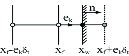
Figure 1: Schematic of lattice node and solid wall boundary.

III Numerical Results and discussions

In this section, we first perform the simulations of some basic three-phase flow problems to validate the proposed LB model coupled with the wetting boundary condition. These typical problems involve partially wettable solid surfaces, which include the spreading of binary drops, the spreading of a compound drop, and the shear of a compound liquid drop. Here we also conduct a detailed comparison between the present numerical results with the analytical solutions or some available results. As an application, at last we use the present method to study the dynamics of a compound drop impact on a solid circular cylinder.

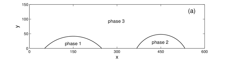
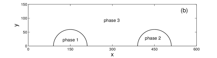
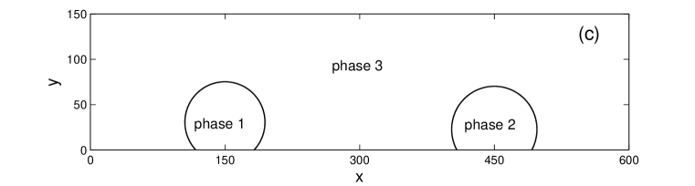
Figure 2: The equilibrium configurations of binary drops on the horizontal substrate with various contact angles, (a) $(\theta_{13},\theta_{23})=(45^{\circ},60^{\circ})$; (b) $(\theta_{13},\theta_{23})=(90^{\circ},90^{\circ})$; (c) $(\theta_{13},\theta_{23})=(135^{\circ},120^{\circ})$.

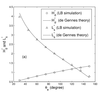
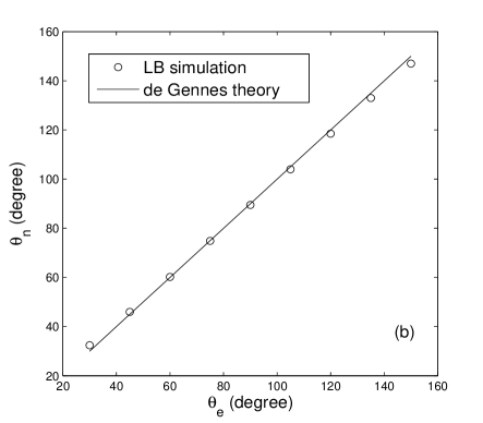
Figure 3: (a) comparison of the equilibrium drop height and spreading length as a function of contact angle between LB simulation and the de Gennes theory Gennes ; (b) the measured contact angle ($\theta_{n}$) versus the theoretical value. The height $H_{d}^{*}$ and length $L_{s}^{*}$ has been normalized by the characteristic scale $R$.

III.1 The spreading of binary drops

We first consider a simple case of the spreading of two liquid drops with different densities on the horizontal substrate, which is a fundamental three-phase flow problem to validate the numerical method Dong . The initial gap between binary drops is assumed to be sufficiently large, such that the interaction between them is very weak, and then can be neglected. In this case, each drop has the equilibrium pattern familiar from the one in two-phase case, which allows us to quantitatively compare the present numerical results with the de Gennes theory Gennes . The physical system considered here is a rectangular domain with a size of $L\times W$, where $L$ and $W$ are the length and width of the domain, and $L/W=4$. Initially, two liquid drops with radius $R=0.1L$ are placed on a partially wetting substrate, and their centers are respectively located at $(x_{1},y_{1})=(0.25L,0)$ and $(x_{2},y_{2})=(0.75L,0)$. In our simulations, the length $L$ is set to be 600 lattice unit, and the order parameters are initialized by

$$\begin{split}c_{1}(x,y)&=0.5+0.5\tanh\frac{2\left[R-(x-x_{1})^{2}-(y-y_{1})^{2}\right]}{D},\\ c_{2}(x,y)&=0.5+0.5\tanh\frac{2\left[R-(x-x_{2})^{2}-(y-y_{2})^{2}\right]}{D},\end{split}$$ (46)

which makes their values to be smooth across the interface. The densities of binary drops are 10 and 5, with an ambient fluid having the density of 1. Some other physical parameters in the simulation are fixed as $D=4$, $\sigma_{12}=\sigma_{13}=\sigma_{23}=0.1$, $\tau_{1}=\tau_{2}=\tau_{g}=0.8$, and $M_{0}=0.01$. The periodic boundary condition is used in the horizontal direction, and we impose the half-way bounce back boundary condition for the bottom and top wall. The wetting boundary condition is also applied at the bottom boundary. When the system is released, it begins to evolve, and eventually reaches its equilibrium state. We mainly focus on the equilibrium configurations of two liquid drops and the contact angle effect.

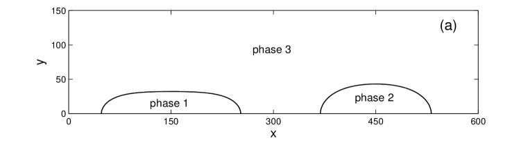
Figure 4: The equilibrium shapes of binary drops at different gravity forces, (a) $g=2\times 10^{-5}$; (b) $g=4\times 10^{-5}$.

Figure 2 depicts the equilibrium shapes of binary liquid drops on the horizontal substrate with three typical groups of contact angles $(\theta_{13},\theta_{23})=(45^{\circ},60^{\circ})$, $(\theta_{13},\theta_{23})=(90^{\circ},90^{\circ})$, and $(\theta_{13},\theta_{23})=(135^{\circ},120^{\circ})$. Note that when $\theta_{13}$ and $\theta_{23}$ have been given, the value of $\theta_{12}$ can be determined from the constraint (39), and here the interface of each drop is marked by the contour levels $c_{i}=0.5$. From Fig. 2, we can observe that each drop intends to adhere the wall, forming a circular cap when the contact angle is less than $90^{\circ}$. And it raises on the wall for the contact angle larger than $90^{\circ}$, while it almost keeps resting on the wall when the contact angle is $90^{\circ}$. The behavior of the drop is in line with the expectation Gennes . In addition, we can see that the equilibrium shape of each drop in the three-phase system is qualitatively consistent with the one that drop alone exists in an ambient fluid. To give a quantitative comparison, we also measure the spreading length ($L_{s}$) between the fluid and substrate and the drop height ($H_{d}$) at the equilibrium state, as illustrated in Fig. 3. According to the de Gennes theory Gennes , the equilibrium spreading length and height can be determined by the following relations,

$$L_{s}=2R\sqrt{\frac{\pi/2}{\theta_{e}-\sin\theta_{e}\cos\theta_{e}}}\sin\theta_{e},~{}~{}H_{d}=R\sqrt{\frac{\pi/2}{\theta_{e}-\sin\theta_{e}\cos\theta_{e}}}(1-\cos\theta_{e}),$$ (47)

where $\theta_{e}$ is the equilibrium contact angle. We plotted the dimensionless equilibrium spreading length and height as a function of the static contact angle in Fig. 3(a), where $L_{s}^{*}$ and $H_{d}^{*}$ have been normalized by the characteristic length $R$. For a comparison, the theoretical results from Eq. (47) are also presented. It is shown that the numerical results are in good agreement with the corresponding analytical solutions. We further measured the numerical contact angle ($\theta_{n}$) based on the geometrical relation $\theta_{n}=2\arctan 2H_{d}/L_{s}$ and presented the results in Fig. 3(b). It is found that the numerical predictions of the contact angles are consistent with the theoretical values.

We now consider the influence of gravity on the equilibrium profile of the above three-phase system. Due to the existing of the gravity, the shape of each drop greatly depends on the relative importance of three force including the gravity force, the surface tension force between fluids, and the adhering force between fluid and solid. For the convenience of discussion, one can introduce a particular length, which is also named as the capillary length denoted by $\gamma^{-1}$. The capillary length is estimated by comparing relative magnitudes of the Laplace pressure and the hydrostatic pressure, and then can be defined by $\gamma^{-1}=\sqrt{\frac{\sigma}{\rho_{l}g}}$ Gennes , where $\sigma$ is the surface tension between two fluids, $\rho_{l}$ is the density of the liquid fluid, and $g$ is the gravitational acceleration. When the drop radius is much smaller than $\gamma^{-1}$, the surface tension force is dominant over the gravity, and then the drop takes on a shape of a circular cap at equilibrium. While when the drop size sufficiently exceeds $\gamma^{-1}$, the gravity force is a crucial force that comes into play in the system, which then results in the formation of a puddle at the equilibrium state Gennes . Based on the de Gennes theory Gennes , the asymptotic thickness ($H$) of a puddle can be analytically expressed as

$$H=2\gamma^{-1}\sin\frac{\theta_{e}}{2}.$$ (48)

We have simulated the spreading of binary drops the horizontal substrate in the presence of the gravity force. In our simulation, the gravity force $\mathbf{G}=(0,-\rho g)$ is applied to all three fluids, and the contact angles ${\theta_{13}}$ and $\theta_{23}$ are assumed to be $90^{\circ}$. The other physical parameters are set as those in the previous situations. Figure 4 shows the equilibrium shapes of binary drops at two different gravitational accelerations. The result with the case of zero gravity is presented in Fig. 2(b). As expected, the drop forms a circular shape at zero gravity, and it intends to spread on the substrate when the gravity is imposed. The shape of the drop becomes flatted with the increase of the gravity, and a puddle can be formed when the gravity is sufficiently large. We also quantitatively measured the asymptotic thickness of each drop from its equilibrium profile, and presented the results with different gravity values in Fig. 5. For a comparison, the corresponding theoretical results given in Eq. (48) are also presented. It can be found from Fig. 5 that our numerical results agree well with the theoretical solutions at large gravity values, while they diverge from the theoretical solutions at small gravity values. These obvious discrepancies can be attributed to the fact that theoretical thickness curve, computed based on Eq. (48) is only valid when the gravity is dominant Dong ; Gennes .

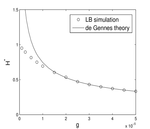
Figure 5: Comparison of the asymptotic thickness as a function of gravity between the LB simulation and the de Gennes theory Gennes . The thickness $H^{*}$ has been normalized by the characteristic length $R$.

III.2 The spreading of a compound drop

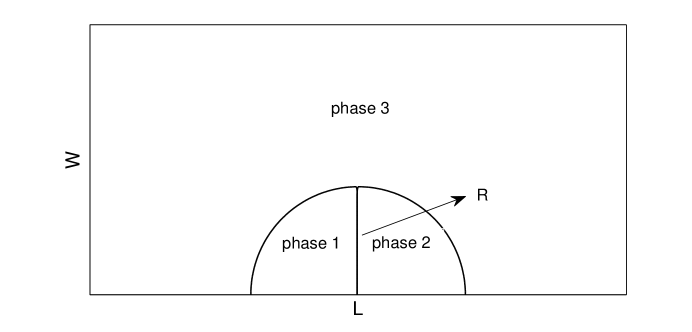
Figure 6: The initial setup of the spreading of a compound drop.

The interaction between two phases in the previous situation is very small. In this subsection, we will consider a case of the spreading of a compound drop on the solid substrate to validate the wetting conditions for ternary fluids, where the interactions among three fluids are very strong, and the equilibrium profile of the system significantly depends on the contact angles among fluids and solid Said ; Ding2 . The initial setup of the physical problem is shown in Fig. 6, in which $L$ and $W$ are the length and width of a rectangle domain, the 1-th and 2-th phase fluids constitute a semi-circle compound drop with the radius $R$ surrounded by the 3-th phase. The boundary conditions are adopted as those of the previous simulation. Some physical parameters in this test are given as $L=2W=300$, $R=60$, and the remaining ones used are set as those of the previous case. Here we focus on the equilibrium shape in a wide range of the contact angles $\theta_{13}$ and $\theta_{23}$ from $30^{\circ}$ to $150^{\circ}$, and the value of the contact angle $\theta_{12}$ can be determined from the relation (39). We first investigated the effect of the contact angle $\theta_{12}$ with a fixed contact angle $\theta_{23}=90^{\circ}$. Figure 7 depicts the equilibrium configurations of a compound liquid drop at various contact angles $\theta_{13}$. We can observe that its equilibrium shape is remarkably affected by the contact angle $\theta_{13}$. For the situation of $\theta_{13}=60^{\circ}$, the 1-th phase intends to spread on the wall, and it also partially moves underneath the 2-th phase, due to the value of $\theta_{13}$ smaller than $90^{\circ}$. With the increase of the $\theta_{13}$, the 1-th phase begins to shrink on the substrate and the region occupied by the phase 1 and the solid is also reduced. As a result, it plumps up with respect to the 2-th phase at equilibrium and the extent increases with the $\theta_{13}$, as can be clearly seen in Figs. 7(b) and (c). When the $\theta_{13}$ is sufficiently large, the 1-th phase intends to migrate away from the solid at equilibrium Dong . In the present numerical experiment, we indeed observe this phenomenon shown in Fig. 7(d), where the 1-th phase moves above the 2-th phase and is no longer in contact with the solid. We also numerically measured the contact angles $\theta_{12}$, $\theta_{13}$ and $\theta_{23}$ between two fluids of the system and the solid, and it is found that all the numerical results are consistent with the initially prescribed values. In addition, we further measured the equilibrium three-phase contact angles $\varphi_{1}$, $\varphi_{2}$, $\varphi_{3}$ at the triple junction, as illustrated in Fig. 7(a). The values of $\varphi_{1}$, $\varphi_{2}$, $\varphi_{3}$ depend on the relative importance of three surface tensions between two fluids of a three-phase system Kim ,

$$\frac{\sin{\varphi_{1}}}{\sigma_{23}}=\frac{\sin{\varphi_{2}}}{\sigma_{13}}=\frac{\sin{\varphi_{3}}}{\sigma_{12}}$$ (49)

and also obviously satisfy the relation $\varphi_{1}+\varphi_{2}+\varphi_{3}=2\pi$. Here the surface tension ratio is fixed to be 1, therefore the analytical solutions for the $\varphi_{1}$, $\varphi_{2}$, $\varphi_{3}$ are all equal to $120^{\circ}$. We also have computed the $\varphi_{1}$, $\varphi_{2}$, $\varphi_{3}$ from the equilibrium profile corresponding to each value of the $\theta_{13}$, and find that all the numerical predictions of the contact angles $\varphi_{i}$ $(i=1,2,3)$ approximate to $120^{\circ}$, which have good agreement with the analytical solutions.

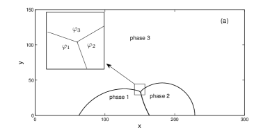
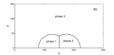
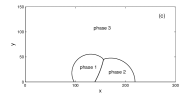
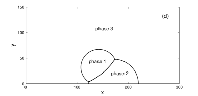
Figure 7: The equilibrium configurations of a compound liquid drop at a fixed contact angle of $\theta_{23}=90^{\circ}$ and various contact angles $\theta_{13}$, (a) $\theta_{13}=60^{\circ}$; (b) $\theta_{13}=90^{\circ}$; (c) $\theta_{13}=120^{\circ}$; (d) $\theta_{13}=150^{\circ}$.

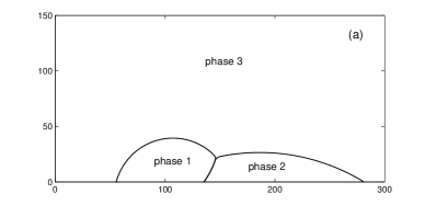
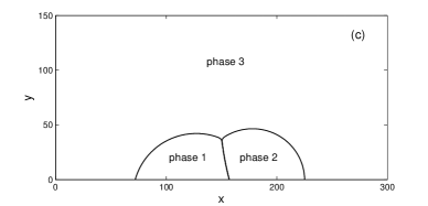
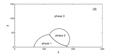
Figure 8: The equilibrium configuration of a compound liquid drop at a fixed contact angle of $\theta_{13}=75^{\circ}$ and various contact angles $\theta_{23}$, (a) $\theta_{23}=30^{\circ}$; (b) $\theta_{23}=60^{\circ}$; (c) $\theta_{23}=90^{\circ}$; (d) $\theta_{23}=135^{\circ}$.

We now focus on the effect of the contact angle $\theta_{23}$ with a fixed value of $\theta_{13}=75^{\circ}$. Figure 8 shows the equilibrium configurations of a compound liquid drop at four typical contact angles $\theta_{23}$. It can be observed that the contact angle $\theta_{23}$ dramatically influences the equilibrium shape of a compound drop. As the $\theta_{23}$ increases, the spreading of the 2-th phase on the wall is reduced, and it becomes more and more plump with respect to the neighbouring phase 1 at the equilibrium. Particularly, when the $\theta_{23}$ is large enough, the 2-th phase would depart from the solid wall and is located on the upside of the 1-th phase fluid. We also quantitatively measured the contact angles $\theta_{ij}$ $(1\leq i<j\leq 3)$ and $\varphi_{i}$ $(1\leq i\leq 3)$, and it is found that the numerical values of the $\theta_{ij}$ are in accordance with the initially given ones, and the values of the $\varphi_{i}$ also conform to Eq. (49).

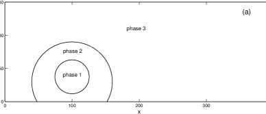
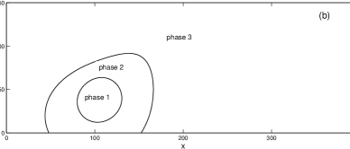
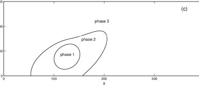
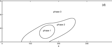
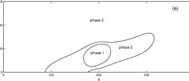
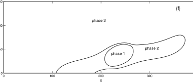
Figure 9: The evolution of interface patterns of a compound liquid drop,(a) t=0; (b) t=10000; (c) t=15000; (d) t=20000; (e) t=25000; (f) t=30000.

III.3 The shear of a compound liquid drop

The shear of a compound drop has extensive applications in the fields of biomedical models of leukocyte Kan and oil-water-gas displacement process Schleizer , and due to the rareness of a suitable numerical approach, very few numerical studies on this subject can be avaiable. In this subsection, we will simulate a compound liquid drop adhering to the wall subject to the shear flow by the three-phase LB model coupled with the present wetting boundary scheme. Initially, a liquid compound drop rests on the substrate of a rectangular domain with the grid $N_{x}\times N_{y}=400\times 150$, and a constant horizontal velocity $U_{0}$ with the value of 0.1 is applied at the upper boundary. The profiles of the order parameters can be initialized by

$$\begin{split}c_{1}(x,y)&=0.5+0.5\tanh\frac{2\left[R_{1}-(x-x_{c1})^{2}+(y-y_{c1})^{2}\right]}{D},\\ c_{2}(x,y)&=0.5+0.5\tanh\frac{2\left[R_{2}-(x-x_{c2})^{2}+(y-y_{c2})^{2}\right]}{D}-c_{1}(x,y),\end{split}$$ (50)

where $R_{1}$ is the radius of the circular drop for the 1-th phase with a value of $25.5$, $(x_{c1},y_{c1})=(37.5,100)$ is its central coordinate, $R_{2}=60$ is the radius of the 2-th phase drop, $(x_{c2},y_{c2})=(30,100)$, and the interface thickness $D$ is 4. The other physical parameters in our simulations are set to be $\rho_{1}=\rho_{2}=\rho_{3}=1$ Yshi , $\sigma_{12}=\sigma_{13}=\sigma_{23}=0.01$, $\tau_{1}=\tau_{2}=\tau_{g}=0.8$, and $M_{0}=0.001$. The problem is periodic in the $x$-direction with the periodic boundary conditions applied for the left and right boundaries. The lower boundary is the solid wall imposed by the no-slip bounce back boundary condition. In addition, to describe the wettability property of the wall material, the present wetting boundary scheme is also applied at the lower boundary. Here three contact angles considered are given as $\theta_{12}=30^{\circ}$, $\theta_{13}=68.53^{\circ}$, and $\theta_{23}=120^{\circ}$. As for the upper boundary, it is velocity boundary which is treat by the nonequilibrium extrapolation scheme proposed by Guo et. al. Guo3 ; Guo4 . The nonequilibrium extrapolation scheme has been successfully applied in single-phase flows Guo1 , and also shows good performance in the study of the two-phase flows Liang2 ; Gong . Here we extend this scheme directly to the three-phase flow situation. The main idea of the scheme is that the distribution function at the boundary is divided into the equilibrium part at the local boundary node and the nonequilibrium part at the neighbouring fluid node Guo3 . Based on this idea Guo3 , the upper boundary condition for three-phase flows can be realized by

$$\begin{split}{f^{i}_{k}}({\mathbf{x}_{u}},t)&=f_{k}^{i,eq}({\bf{x}}_{u},t)+f_{k}^{i,neq}({\bf{x}}_{f},t),~{}~{}i=1,~{}2,\\ {g_{k}}({\mathbf{x}_{u}},t)&=g_{k}^{eq}({\bf{x}}_{u},t)+g_{k}^{neq}({\bf{x}}_{f},t),\end{split}$$ (51)

where ${\mathbf{x}_{u}}$ is the node at the upper boundary, ${\mathbf{x}_{f}}$ is its neighbouring fluid node, the nonequilibrium parts $f_{k}^{i,neq}({\bf{x}}_{f},t)$ and $g_{k}^{neq}({\bf{x}}_{f},t)$ can be given by

$$\begin{split}f_{k}^{i,neq}({\bf{x}}_{f},t)&={{f^{i}_{k}}(\textbf{x}_{f},t)-f_{k}^{i,eq}(\textbf{x}_{f},t)},~{}~{}i=1,~{}2,\\ g_{k}^{neq}({\bf{x}}_{f},t)&={{g_{k}}(\textbf{x}_{f},t)-g_{k}^{eq}(\textbf{x}_{f},t)},\end{split}$$ (52)

that have been known, and the equilibrium parts $f_{k}^{i,eq}({\bf{x}}_{u},t)$ and $g_{k}^{eq}({\bf{x}}_{u},t)$ can be expressed as

$$f_{k}^{i,eq}({\bf{x}}_{u},t)=\left\{\begin{array}[]{ll}c_{i}({\bf{x}}_{u},t)+({\omega_{k}}-1)\eta{\mu_{i}}({\bf{x}}_{u},t),&\textrm{ $k=0$}\\ {\omega_{k}}\eta{\mu_{i}}({\bf{x}}_{u},t)+{\omega_{k}}c_{i}({\bf{x}}_{u},t){{{\textbf{e}_{k}}\cdot{\bf{u}}}({\bf{x}}_{u},t)\over{c_{s}^{2}}},&\textrm{ $k\neq 0$},~{}~{}i=1,~{}2,\end{array}\right.$$ (53a)

$$g_{k}^{eq}({\bf{x}}_{u},t)=\left\{\begin{array}[]{ll}{p({\bf{x}}_{u},t)\over{c_{s}^{2}}}({\omega_{k}}-1)+\rho({\bf{x}}_{u},t){s_{k}}[{\bf{u}}({\bf{x}}_{u},t)],&\textrm{ $k=0$},\\ {p({\bf{x}}_{u},t)\over{c_{s}^{2}}}{\omega_{k}}+\rho({\bf{x}}_{u},t){s_{k}}[{\bf{u}}({\bf{x}}_{u},t)],&\textrm{ $k\neq 0$},\\ \end{array}\right.$$ (53b)

where ${\bf{u}}({\bf{x}}_{u},t)=(U_{0},0)$, and the unknown macroscopic quantities $c_{i}({\bf{x}}_{u},t)$, $\mu({\bf{x}}_{u},t)$, $p({\bf{x}}_{u},t)$, and $\rho({\bf{x}}_{u},t)$ in Eqs. (53a) and (53b) are determined by the interpolation $\chi({\bf{x}}_{u},t)=\chi({\bf{x}}_{f},t)$, where $\chi$ represent the above quantities. Figure 9 depicts the time evolution of interface patterns of a compound liquid drop. It is found that the drop of the 2-th phase has a deformation under the shear force of its surrounding fluid, and becomes more and more elongated with time along the direction of the shear velocity. Obviously, the upper portion of the drop moves much faster than its lower portion. Also, it is found that the inner drop of the 1-th phase undergoes an interfacial deformation, while the extent is obviously reduced due to the small shear interaction. Our present numerical results are qualitatively consistent with those of the previous study Yshi .

III.4 A compound drop impact on a solid circular cylinder

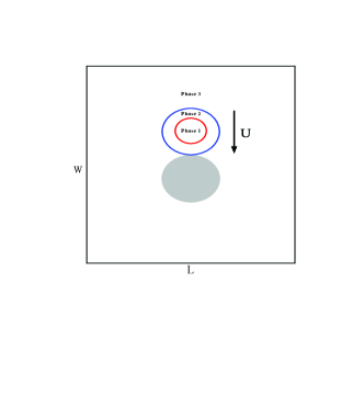
Figure 10: The schematic illustration for a compound drop impact on a solid circular cylinder.

At last, to show the versatility of the present wetting boundary condition in dealing with three-phase fluid-solid systems, we consider a complex problem of a compound drop impact on a solid circular cylinder. Drop impact on a flat or curved substrate has great relevance to many technical applications, such as oil recovery, ink jet printing and and coating Yarin ; Lefebvre . Additionally, it can also serve as an important multiphase benckmark problem, which involves very fascinating interfacial phenomena, including spreading, splashing, bouncing, etc Yarin . Due to its importance, drop impact on a solid target has been investigated extensively using the experimental and numerical approaches Fakhari ; Yarin ; Bakshi ; Ding3 . However, the studies on this subject are almostly limited to the two-phase situation Fakhari ; Bakshi ; Ding3 , and the mechanism of drop impact, especially in the case of a compound drop, has been far from well understood. Actually, to the best of our knowledge, there is no literature avaiable on the numerical study of a compound drop impact on solid. To fill the gap, here we will use the phase-field-based three-phase LB model coupled with the present wetting boundary scheme to numerically investigate the impact of a compound drop onto a solid circular cylinder.

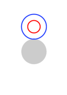
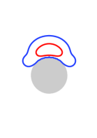
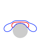
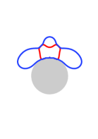
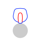
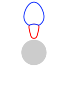
Figure 11: Snapshots of a compound drop impact on a cylindrical solid wall with $We=21.6$ and $\theta_{13}=150^{\circ}$. The dimensionless time instants from the left pattern to the right are 0, 0.5, 2.0, 4.0, 6.0, 9.0.

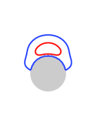
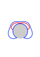
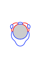
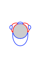
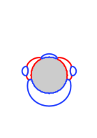
Figure 12: Snapshots of a compound drop impact on a cylindrical solid wall with $We=21.6$ and $\theta_{13}=30^{\circ}$. The dimensionless time instants from the left pattern to the right are 0, 0.5, 2.0, 4.0, 6.0, 10.0.

The schematic of the physical problem is illustrated in Fig. 10, where $L$ and $W$ are the length and width of the rectangular domain, and a solid circular cylinder with the radius of $L/8$ is centered at $(0.5L,0.5L)$. Initially a compound drop consisting of phases 1 and 2, in a shape of circle, is placed on the top of a solid circular cylinder. The initial velocity in the vertical direction with the value of $U$ is imposed for the compound drop without the consideration of the gravity, and then it will impact onto the solid surface. Similar to the two-phase case Fakhari ; Ding3 , this problem can be characterized by the wall wettability in terms of the contact angles and two group of dimensionless parameters: the Reynolds number ($Re$) and the Weber number ($We$), which can be defined respectively as

$$Re=\frac{\xi U}{\bar{\nu}},$$ (54)

and

$$We=\frac{\bar{\rho}\xi U^{2}}{\bar{\sigma}},$$ (55)

where $\xi$ is the diameter of the compound drop given by $L/4$, $\bar{\nu}$, $\bar{\rho}$ are the viscosity and density of the compound drop by averaging those of two fluids, i.e., $\bar{\nu}=0.5(\nu_{1}+\nu_{2})$, $\bar{\rho}=0.5(\rho_{1}+\rho_{2})$, and $\bar{\sigma}$ is the average surface tension computed by $0.5(\sigma_{13}+\sigma_{23})$. Here we choose $\xi$ and $U$ as the characteristic length and velocity, and then the characteristic time is given by $\xi/U$.

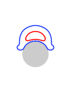
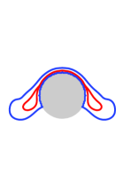
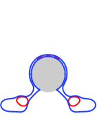
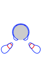
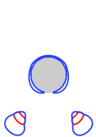
Figure 13: Snapshots of a compound drop impact on a cylindrical solid wall with $We=86.4$ and $\theta_{13}=30^{\circ}$. The dimensionless time instants from the left pattern to the right are 0, 0.5, 2.0, 4.0, 5.0, 7.0.

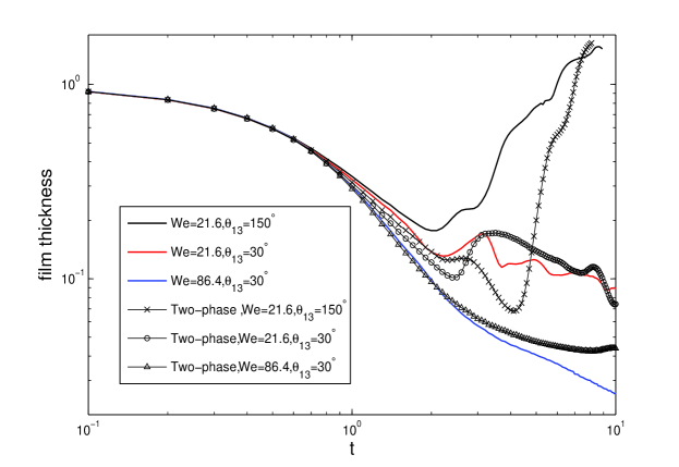
Figure 14: Temporal evolution of the normalized film thickness ($h/\xi$) at different Weber numbers and contact angles.

The simulation was carried out in a uniform mesh of $L\times W=240\times 280$ with periodic boundary conditions at all boundaries. The bounce back no-slip and wetting boundary conditions are applied on the solid surface of the circular cylinder. The profiles of the order parameters can be initialized by

$$\begin{split}c_{1}(x,y)&=0.5+0.5\tanh\frac{2[R_{1}-\sqrt{(x-x_{c})^{2})+(y-y_{c})^{2}}]}{D},\\ c_{2}(x,y)&=0.5+0.5\tanh\frac{2[R_{2}-\sqrt{(x-x_{c})^{2})+(y-y_{c})^{2}}]}{D}-c_{1}(x,y),\end{split}$$ (56)

where $(x_{c},y_{c})=(0.5L,0.75L)$ is the center of the compound drop, $R_{1}$, $R_{2}$ are the radii of the compound drop and the inner drop that are set to be $L/8$ and $L/16$. In the simulations, the physical properties of the fluids are assumed to be $\theta_{13}=\theta_{23}$, $\nu_{1}:\nu_{2}:\nu_{3}=1:1:1$, and $\sigma_{12}:\sigma_{13}:\sigma_{23}=1:1:1$. The contact angle $\theta_{12}$ and the Reynolds number are fixed to be $90^{\circ}$ and 600. Then the remaining physical parameters are given as $U=0.06$, $\rho_{1}=\rho_{2}=10.0$, $\rho_{3}=1.0$, $M_{1}=M_{2}=0.1$, and $\tau_{1}=\tau_{2}=0.8$. Here we mainly focus on the effects of the contact angle $\theta_{13}$, and the Weber number by adjusting the value of the surface tension. Figure 11 depicts snapshots of a compound drop impact dynamics on a superhydrophobic cylinder with $\theta_{13}=150^{\circ}$ and $We=21.6$. It can be observed that, due to the inertia effect, the compound drop firstly spreads on the solid cylinder, while its two-side tails are not in contact with the surface due to the hydrophobicity property. After that, the compound drop retracts with time and the superhydrophobicity becomes to dominate over the inertia effect as the downward velocity is reduced, which results in the eventual rebound of the compound drop and completely detaches from the solid cylinder. The rebound scenario is similar to the two-phase situation that a single drop impacts on a flat or curve hydrophobic surface Ding3 ; Yarin . To examine the effect of the surface wettability, we also simulated the case with the hydrophilic surface $(\theta_{13}=30^{\circ})$ and $We=21.6$, and showed the results in Fig. 12. As can be seen from Fig. 12 that the compound drop takes on a distinctive behaviour. It spreads continuously along the edge of the solid cylinder, and then covers over the whole surface after a certain time of evolution. The compound drop goes on to move downward and portion of it hangs from the cylinder surface. Under the action of the surface tension force, it has mild shrinkage and finally reaches its equilibrium state. From the perspective of each phase, we can observe that the inner drop consisting of the 1-th phase breaks up into two symmetrical daughter drops, while the outer drop consisting of the 2-th phase is stretched into multiple drops, which cannot be found in the above situation. We also consider the effect of the Weber number on the impact dynamics. Figure 13 shows the snapshots of a compound drop impact on a cylindrical solid wall with a large $We$ of 86.4 and $\theta_{13}=30^{\circ}$. Comparatively, the compound drop also spreads along the edge of the solid cylinder at the early time. Due to the larger Weber number, however, the inertia pulling force prevails over the surface tension force. Then, two thick liquid tails are formed at the side, in addition to the liquid film around the solid surface. Finally, the film breaks up, leading to the release of two daughter compound drops. We should also emphasize that the breakup phenomena of the compound drop cannot be observed for a small Weber number.

The film thickness on the top of the solid cylinder is a concerned physical quantity in the study of the drop impact dynamics Fakhari ; Bakshi . Here we also measured the film thickness of the compound drop with different Weber numbers and contact angles, and showed the dimensionless results in Fig. 14. Due to the lack of the research on this subject, we cannot quantitatively compare the present results with the available experimental data or the numerical results. For a comparsion, however, we presented in Fig. 14 the results of a single drop impact on the same cylinder, which are derived from the simulations of the present three-phase LB method by seting $c_{1}=0$. It can be found from Fig. 14 that for all the cases, the film thickness of the compound drop has a uniform curve at the initial stage, which is also in line with that of the two-phase simulation Fakhari . Then the noticeable difference between them can be observed. For the superhydrophobic surface, the film thickness of the compound drop continues to decrease at first and then has a rapid increase with time, which can be attribute to that the rebound phenomenon occurs for the compound drop. While for the hydrophilic surface, the file thickness of the compound drop firstly has a relatively rapid decrease and then undergoes a smooth change with time. As for the hydrophilic surface with a larger We, the film thickness undergoes a rapid decline with time until it reaches a residual value. In addition, the comparison between the film curves of the compound drop and single drop shows that they have qualitatively similar variation tendencies under the same condition, but are quantitatively different.

IV Summary

Multiphase flows involving multiple fluid components and solid boundary are frequently encountered in the engineering applications. To simulate such flows, how to describe the interactions among multiple fluids and solid surface is a crucial problem. In this paper a suitable wetting boundary scheme that describe the fluid-solid interaction in the framework of the lattice Boltzmann method based on the phase-field theory is proposed. Due to the particular choice of the wall free energy, the proposed wetting boundary scheme can preserve the reduction consistency property with the binary one. Coupled with this wetting boundary scheme, a lattice Boltzmann model for three-phase flows that also satisfies algebraical and dynamical consistency properties is used to simulate the ternary fluid flows in contact with solid wall. Numerical examples include the spreading of binary drops on the substrate, the spreading of a compound drop on the substrate, and the shear of a compound drop on the substrate. It is shown that the numerical results of these flows agree well with the theoretical results or some available data for a broad range of contact angles, which provides a good validation of the present wetting boundary scheme. As an application, we further use the lattice Boltzmann tenary fluid model coupled with the wetting boundary condition to study a compound drop impact on the solid cylinder, which has not been considered before in the literature. It is found that the compound drop dynamics can be significantly influenced by the wettability of the cylinder surface and the Weber number, and some interesting interfacial phenomena, including spreading, breakup, rebound, are also observed in the simulation results. Our present discussion focuses on the Cahn-Hilliard phase field model, and actually, the generalized wetting boundary scheme here is appropriate for the Allen-Cahn type phase field model. Finally, we anticipate that our numerical method will be useful to microfluidics, material science, and oil recovery industry.

References

- (1) A. Maghzi, S. Mohammadi, M.H. Ghazanfari, R. Kharrat, M. Masihi, Monitoring wettability alteration by silica nanoparticles during water flooding to heavy oils in five-spot systems: A pore-level investigation, Exp. Therm. Fluid Sci. 40 (2012) 168-176.
- (2) H. Li et. al., A review of water flooding issues in the proton exchange membrane fuel cell, J. Power Sources 178 (2008) 103-117.
- (3) R. Seemann, M. Brinkmann, T. Pfohl and S. Herminghaus, Droplet based microfluidics, Rep. Prog. Phys. 75 (2012) 016601.
- (4) H. K. Zhao, T. Chan, B. Merriman, S. Osher, A variational level set approach to multiphase motion, J. Comput. Phys. 127 (1996) 179-195.
- (5) R.I. Saye and J.A. Sethian, The Voronoi implicit interface method for computing multiphase physics, Pro. Natl. Acad. Sci. 108 (2011) 19498-19503.
- (6) R. Bonhomme, J. Magnaudet, F. Duval and B. Piar, Inertial dynamics of air bubbles crossing a horizontal fluid-fluid interface, J. Fluid Mech. 707 (2012) 405-443.
- (7) N. Tofighi and M. Yildiz, Numerical simulation of single droplet dynamics in three-phase flows using ISPH, Comput. Math. Appl. 66 (2013) 525-536.
- (8) H. Garcke, B. Nestler and B. Stoth, A multiphase field concept: numerical simulations of moving phase boundaries and multiple junctions, SIAM J. Appl. Math. 60 (1999) 295-315.
- (9) F. Boyer, C. Lapuerta, Study of a three component Cahn-Hilliard flow model, ESAIM: Math. Model. Numer. Anal. 40 (2006) 653-687.
- (10) J. Kim, Phase field computations for ternary fluid flows, Comput. Methods Appl. Mech. Engrg. 196 (2007) 4779-4788.
- (11) F. Boyer, C. Lapuerta, S. Minjeaud, B. Piar, and M. Quintard, Cahn-Hilliard/Navier-Stokes model for the simulation of of three-phase flows, Transp. Porous Media 82 (2010) 463-483.
- (12) M. Said, M. Selzer, B. Nestler, D. Braun, C. Greiner and H. Garcke, A phase-field approach for wetting phenomena of multiphase droplets on solid surfaces, Langmuir 30 (2014) 4033-4039.
- (13) S. Dong, Wall-bounded multiphase flows of N immiscible incompressible fluids: Consistency and contact-angle boundary condition, J. Comput. Phys. 338 (2017) 21-67.
- (14) D. M. Anderson, G. B. McFadden, and A. A. Wheeler, Diffuse-interface methods in fluid mechanics, Annu. Rev. Fluid Mech. 30 (1998) 139-165.
- (15) Z. L. Guo, C. Shu, Lattice Boltzmann method and its applications in engineering, World Scientific Singapore, 2013.
- (16) A. K. Gunstensen, D. H. Rothman, S. Zaleski, and G. Zanetti, Lattice Boltzmann model of immiscible fluids, Phys. Rev. A 43 (1991) 4320.
- (17) X. Shan and H. Chen, Simulation of nonideal gases and liquid-gas phase transitions by the lattice Boltzmann equation, Phys. Rev. E 49 (1994) 2941.
- (18) M. Swift, W. Osborn, and J. Yeomans, Lattice Boltzmann simulation of nonideal fluids, Phys. Rev. Lett. 75 (1995) 830.
- (19) X. He, S. Chen, and R. Zhang, A lattice Boltzmann scheme for incompressible multiphase flow and its application in simulation of Rayleigh-Taylor instability, J. Comput. Phys. 152 (1999) 642-663.
- (20) T. Lee and L. Liu, Lattice Boltzmann simulations of micron-scale drop impact on dry surfaces, J. Comput. Phys. 229 (2010) 8045-8063.
- (21) H. Liang, B. C. Shi, Z. L. Guo, Z. H. Chai, Phase-field-based multiple-relaxation-time lattice Boltzmann model for incompressible multiphase flows, Phys. Rev. E 89 (2014) 053320.
- (22) H. Liang, Z. H. Chai, B. C. Shi, Z. L. Guo, and T. Zhang, Phase-field-based lattice Boltzmann model for axisymmetric multiphase flows, Phys. Rev. E 90 (2014) 063311.
- (23) A. Fakhari, D. Bolster, Diffuse interface modeling of three-phase contact line dynamics on curved boundaries: A lattice Boltzmann model for large density and viscosity ratios, J. Comput. Phys. 334 (2017) 620-638.
- (24) H. Liu, Q. J. Kang, C. R. Leonardi et. al., Multiphase lattice Boltzmann simulations for porous media applications, Comput. Geosci. 20 (2016) 777-805
- (25) Q. Li, H. K. Luo, Q. J. Kang, Y. L. He, Q. Chen, Q. Liu, Lattice Boltzmann methods for multiphase flow and phase-change heat transfer, Prog. Energy Combust. Sci. 52 (2016) 62-105.
- (26) A. Lamura, G. Gonnella, J. Yeomans, A lattice Boltzmann model of ternary fluid mixtures, Europhys. Lett. 45 (1999) 314.
- (27) Q. Li, A. J. Wagner, Symmetric free-energy-based multicomponent lattice Boltzmann method, Phys. Rev. E 76 (2007) 036701.
- (28) C. Semprebon, T. Kruger, and H. Kusumaatmaja, Ternary free-energy lattice Boltzmann model with tunable surface tensions and contact angles, Phys. Rev. E 93 (2016) 033305.
- (29) H. Chen, B. M. Boghosian, P. V. Coveney, and M. Nekovee, A ternary lattice Boltzmann model for amphiphilic fluids, Proc. R. Soc. London, Ser. A 456 (2000) 2043-2057.
- (30) M. Nekovee, P. V. Coveney, H. Chen, and B. M. Boghosian, Lattice-Boltzmann model for interacting amphiphilic fluids, Phys. Rev. E 62 (2000) 8282.
- (31) I. Halliday, A.P. Hollis, C.M. Care, Lattice Boltzmann algorithm for continuum multicomponent flow, Phys. Rev. E 76 (2007) 026708.
- (32) T.J. Spencer, I. Halliday, C.M. Care, Lattice Boltzmann equation method for multiple immiscible continuum fluids, Phys. Rev. E 82 (2010) 066701.
- (33) S. Leclaire, M. Reggio, J. Trepanier, Progress and investigation on lattice Boltzmann modeling of multiple immiscible fluids or components with variable density and viscosity ratios, J. Comput. Phys. 246 (2013) 318-342.
- (34) H. Liang, B. C. Shi, and Z. H. Chai, Lattice Boltzmann modeling of three-phase incompressible flows, Phys. Rev. E. 93 (2016) 013308.
- (35) H. Liang, Q. X. Li, B. C. Shi, and Z. H. Chai, Lattice Boltzmann simulation of three-dimensional Rayleigh-Taylor instability, Phys. Rev. E. 93 (2016) 033113.
- (36) Z. L. Guo, C. G. Zheng, and B. C. Shi, Discrete lattice effects on the forcing term in the lattice Boltzmann method, Phys. Rev. E 65 (2002) 046308.
- (37) B. C. Shi and Z. L. Guo, Lattice Boltzmann model for nonlinear convection-diffusion equations, Rev. E 79 (2009) 016701.
- (38) Z. H. Chai, B. C. Shi, Z. L. Guo, A multiple-relaxation-time lattice Boltzmann model for general nonlinear anisotropic convection-diffusion equations, J. Sci. Comput. 69 (2016) 355-390.
- (39) Y. Shi, X. P. Wang, Modeling and simulation of dynamics of three-component flows on solid surface, Japan J. Indust. Appl. Math. 31 (2014) 611-631.
- (40) Q. Zhang, X. P. Wang, Phase field modeling and simulation of three-phase flow on solid surfaces, J. Comput. Phys. 319 (2016) 79-107.
- (41) C. Zhang, H. Ding, P. Gao, Y. Wu, Diffuse interface simulation of ternary fluids in contact with solid, J. Comput. Phys. 309 (2016) 37-51.
- (42) Z. L. Guo, C. G. Zheng, ang B. C. Shi, Non-equilibrium extrapolation method for velocity and pressure boundary conditions in the lattice Boltzmann method, Chin. Phys. 11 (2002) 366-374.
- (43) P.G. de Gennes, F. Brochard-Wyart, D. Quere, Capillarity and Wetting Phenomena, Springer, 2003.
- (44) H. C. Kan, H. S. Udaykumar, W. Shyy, T. Roger, Hydrodynamics of a compound drop with application to leukocyte modeling, Phys. Fluids 10 (1998) 760-774.
- (45) A. D. Schleizer, R. T. Bonnecaze, Displacement of a two-dimensional immiscible droplet adhering to a wall in shear and pressure-driven flows, J. Fluid Mech. 383 (1999) 29-54.
- (46) Z. L. Guo, C. G. Zheng, and B. C. Shi, An extrapolation method for boundary conditions in lattice Boltzmann method, Phys. Fluids 14 (2002) 2007.
- (47) S. Gong, P. Cheng, X. Quan, Lattice Boltzmann simulation of droplet formation in microchannels under an electric field, Int. J. Heat Mass Tran. 53 (2010) 5863-5870.
- (48) A. L. Yarin, Drop impact dynamics: splashing, spreading, receding, bouncing…, Annu. Rev. Fluid Mech. 38 (2006) 159-192.
- (49) A. H. Lefebvre, V. G. McDonell, Atomization and sprays, CRC Press, 2017.
- (50) S. Bakshi, I. Roisman, and C. Tropea, Investigations on the impact of a drop onto a small spherical target, Phys. Fluids 19 (2007) 032102.
- (51) H. R. Liu, H. Ding, A diffuse-interface immersed-boundary method for two-dimensional simulation of flows with moving contact lines on curved substrates, J. Comput. Phys. 294 (2015) 484-502.