Qubit models of weak continuous measurements

Abstract

In this paper we approach the theory of continuous measurements and the associated unconditional and conditional (stochastic) master equations from the perspective of quantum information and quantum computing. We do so by showing how the continuous-time evolution of these master equations arises from discretizing in time the interaction between a system and a probe field and by formulating quantum-circuit diagrams for the discretized evolution. We then reformulate this interaction by replacing the probe field with a bath of qubits, one for each discretized time segment, reproducing all of the standard quantum-optical master equations. This provides an economical formulation of the theory, highlighting its fundamental underlying assumptions.

I Introduction and Motivation

The strength of a projective measurement is made known in weakness. Although we are taught from youth that quantum measurements project the target system onto an eigenstate of the measured observable as an irreducible action, closer inspection reveals a more nuanced reality. Measurements involve coupling quantum systems to macroscopic devices via finite-energy interactions, these devices have finite temporal resolution, and a host of imperfections lead to encounters with the classical world that violate unitarity without conforming to the projective-measurement mold.

Of course, in many scenarios these discrepancies are fleeting and the projective description is all that is needed—and sometimes all that can be observed! Modern experiments, however, show projective measurements for what they are, and if we are to glory in this revelation, we need tools like the theory of quantum trajectories, which generalizes measurement projection to weak, continuous monitoring of a quantum system.

Consider using a transition-edge sensor to detect photons. As a photon is absorbed by the detector, the output current begins to drop. At first it is difficult to tell the difference between a photon and thermal fluctuations, but as the current continues to drop we become more and more confident of the detection prognosis until we have integrated enough current deficiency to announce a detection. The accumulating current deficiency is the result of a continuous sequence of weak measurements (sometimes called gentle or fuzzy), where the name signifies that each measurement outcome (in this case output current integrated over a short time interval) contains little information about the system being measured and consequently only gently disturbs that system. Many repetitions of such weak measurements, however, do have an appreciable effect upon the system, sometimes as dramatic as a projective measurement. Because these measurements are nearly continuous, differential equations are used to track the cumulative effect on the system, and because quantum theory tells us the measurement results are random, these differential equations are stochastic.

The system’s time-dependent state (or some expectation value thereof) conditioned on a continuous measurement record is called a quantum trajectory in the continuous-measurement literature. Physically, this continuous measurement record is written on successive probes that interact weakly with the system. The stochastic differential equations that generate quantum trajectories take a variety of forms, going by names such as stochastic Schrödinger equations, quantum-filtering equations, or in this paper stochastic master equations (SMEs). A great deal of attention has been devoted both to deriving stochastic equations for and to observing trajectories in a variety of physical systems, e.g., cavity QED Hood et al. (1998), circuit QED (superconducting systems) Gambetta et al. (2008); Boissonneault et al. (2008); Murch et al. (2013), fermionic systems Goan and Milburn (2001); Oxtoby et al. (2005, 2008), and mechanical systems Milburn et al. (1994); Hopkins et al. (2003); Ruskov et al. (2005); Jacobs et al. (2007).

The ability to resolve these subprojective effects opens up many possibilities, including feedback protocols and continuous-time parameter estimation. An example of feedback control is continuous-time quantum error correction. Ahn et al. (2002) investigated using continuous-time quantum measurements for this purpose, thus pioneering a fruitful line of research Sarovar et al. (2004); Ahn et al. (2004); Gregoratti and Werner (2004); van Handel and Mabuchi (2005); Chase et al. (2008); Mabuchi (2009); Lidar and Brun (2013); Nguyen et al. (2015); Hsu and Brun (2016). Feedback control additionally allows one to view weak measurements as building blocks for constructing other generalized measurements, as explored by Brun and collaborators Oreshkov and Brun (2005); Varbanov and Brun (2007); Florjanczyk and Brun (2015, 2014). Continuous weak measurements have also been pressed into service for parameter and state estimation Mabuchi (1996); Gambetta and Wiseman (2001); Chase and Geremia (2009); Gammelmark and Mølmer (2013); Kiilerich and Mølmer (2014, 2016); Gong and Cui (2017). One notable example is the single shot tomography of an ensemble of identically prepared qubits Cook et al. (2014).

Error correction, parameter estimation, and state tomography are important subjects in quantum computation and information. Unfortunately, much of the literature on continuous weak measurements, which would otherwise be of interest to this community, suffers from needlessly arcane terminology and interpretations. We take the refiner’s fire to trajectory theory, revealing a foundation of finite-dimensional probe systems, unitary gates between the system and successive probes, and quantum operations to describe the system state after the probe is measured—all three familiar to the quantum information scientist of today. This process also distills the essence of trajectory theory from its origins in field-theoretic probes, yielding insights that can be appreciated even by veterans of the subject. A particularly useful tool that arises naturally within our approach is the quantum circuit diagram, and we take pains throughout our presentation to illustrate relevant principles with this tool.

Of all the prior work on this subject, our paper is most related to—and indeed inspired by—Brun’s elegant work on qubit models of quantum trajectories Brun (2002). In Sections III and V we describe the connection between his work and ours. Looking further back to the origin of this line of research, one might identify an important precedent in the work Scully and Lamb (1967) of the great theorists, Scully and Lamb (Lamb also did experiments), in which they considered systems interacting with a spin bath. The mathematics literature has a related body of work that studies approximating Fock spaces with chains of qubits known as “toy Fock spaces” Meyer (1986); Attal (2002); Gough and Sobolev (2004); Gough (2004); Attal and Pautrat (2005, 2006); Belton (2008); Bouten et al. (2009); Attal and Nechita (2011).

The physics and mathematical-physics communities have a rich history of deriving the stochastic equations of motion for a system subject to a continuous measurement. So rich, in fact, that these equations have been discovered and rediscovered many times. Historically, the theory was developed in the 80’s and early 90’s by a number of authors: Mensky (1979, 1993), Belavkin (1980), Srinivas and Davies (1981), Braginskiĭ and Khalili (1995), Barchielli et al. (1982), Gisin (1984), Diósi (1986, 1988), Caves Caves (1986, 1987), Caves and Milburn Caves and Milburn (1987), Milburn Wiseman and Milburn (1993a), Carmichael (1993a), Dalibard et al. (1992), and Wiseman Wiseman and Milburn (1993a). Most recently Korotkov (1999, 2001) developed a treatment of continuous measurements; this treatment, which Korotkov dubbed ‘quantum Bayesian theory,’ is notable in that it is based on baths and detection processes that are characteristic of condensed systems.

Many other good references on the topic are available for the interested reader. We recommend the following articles: Brun (2002), Jacobs and Steck (2006), Wiseman’s PhD thesis Wiseman (1994a), and for the mathematically inclined reader, Bouten et al. (2009, 2007). Helpful books include Carmichael (1993a), Carmichael (2008), Wiseman and Milburn (2010), and Jacobs (2014).

This paper is structured as follows: Section II lays out our notational conventions. Section III gives a unified description of strong and weak measurements via ancilla-coupled measurements, followed by quantum-circuit depictions of the iterated interactions that limit to continuous quantum measurements and their relation to Markovicity. Section IV develops the continuous-measurement theory in terms of a system undergoing successive weak interactions with a probe field.

Sections V, VI and VII are the heart of the paper: they show how to replace a probe field with probe qubits in constructing quantum trajectories, and they explore the consequences of changing the parameters of the formalism, i.e., using different probe initial states, different interaction unitaries, and different measurements on the probes. Section V contains the first derivation of a SME in our model, focusing on the vacuum SMEs. These arise when probe initial states are vacuum (ground state for probe qubits); the probe undergoes a weak interaction with the system and then experiences one of several kinds of measurements, which lead to different quantum trajectories. The theme of Section V is thus exploring the effect of different kinds of measurements on the probes. Section VI considers the Gaussian SMEs, in which a probe field starts in a Gaussian state, undergoes a weak interaction with the system, and then is subjected to homodyne measurements. The theme of this section is thus exploring the effect of different probe initial states, but the main contribution of this section is a technique to accommodate all the Gaussian field states in probe qubits and to show that, since qubits have too small a Hilbert space to achieve this by only changing the initial state, one must also modify aspects of the weak system/probe interaction unitary. Section VII explores a radical departure that allows interactions between the probe qubits and the system that are strong, but occur randomly.

As an aid to intuition, Sec. VIII presents visualizations of numerical solutions to some of the SMEs derived in the previous sections. Finally, Sec. IX summarizes lessons learned from our approach and suggests promising related approaches.

II Notational Conventions

Confusion can arise when denoting the states of quantum-field modes and two-level systems (qubits) in the same context. In particular, that $a\left|{n}\right\rangle=\sqrt{n}\left|{n-1}\right\rangle$ and thus $a\left|{1}\right\rangle=\left|{0}\right\rangle$, yet $\sigma_{-}\left|{0}\right\rangle=\left|{1}\right\rangle$, can lead to momentary confusion and even persistent perplexity. The standard qubit states are the eigenstates of $\sigma_{z}=\left|{0}\middle\rangle\middle\langle{0}\right|-\left|{1}\middle\rangle\middle\langle{1}\right|=\sum_{a=0,1}(-1)^{a}\left|{a}\middle\rangle\middle\langle{a}\right|$; since the qubit Hamiltonian is often proportional to $\sigma_{z}$—this is why one chooses $\left|{0}\right\rangle$ and $\left|{1}\right\rangle$ to be the standard states—it is natural to regard $\left|{1}\right\rangle$ (eigenvalue $-1$ of $\sigma_{z}$) as the ground state and $\left|{0}\right\rangle$ (eigenvalue $+1$) as the excited state. In doing so, one is allowing the multiplicative label $(-1)^{a}$ to trump the bitwise label $a$, which gives an opposite hint for what should be labeled ground and excited.

To allay this confusion, one good practice would be to label the standard qubit states by the eigenvalue, $(-1)^{a}$, of $\sigma_{z}$, but instead we choose the more physical labeling of $\left|{g}\right\rangle=\left|{1}\right\rangle$ as the “ground state” and $\left|{e}\right\rangle=\left|{0}\right\rangle$ as the “excited state.” In this notation, $\sigma_{-}\left|{e}\right\rangle=\left|{g}\right\rangle$, as expected; this notation plays well with the correspondence we develop between field modes and two-level systems. Our notation is illustrated in Fig. 1. As a further check on confusion, we often label the vacuum state of a field mode as $\left|{\rm vac}\right\rangle$ instead of $\left|{0}\right\rangle$.

Some useful relations between qubit operators are given below:

$$\begin{split}\sigma_{+}&=\left|{e}\middle\rangle\middle\langle{g}\right|=\left|{0}\middle\rangle\middle\langle{1}\right|=\mbox{$\frac{1}{2}$}(\sigma_{x}+i\sigma_{y})\,,\\ \sigma_{-}&=\left|{g}\middle\rangle\middle\langle{e}\right|=\left|{1}\middle\rangle\middle\langle{0}\right|=\mbox{$\frac{1}{2}$}(\sigma_{x}-i\sigma_{y})\,,\\ \sigma_{x}&=\sigma_{+}+\sigma_{-}=\left|{e}\middle\rangle\middle\langle{g}\right|+\left|{g}\middle\rangle\middle\langle{e}\right|\,,\\ \sigma_{y}&=-i\sigma_{+}+i\sigma_{-}=-i\left|{e}\middle\rangle\middle\langle{g}\right|+i\left|{g}\middle\rangle\middle\langle{e}\right|\,,\\ \sigma_{z}&=\left|{e}\middle\rangle\middle\langle{e}\right|-\left|{g}\middle\rangle\middle\langle{g}\right|\,,\\ [\sigma_{-},\sigma_{+}]&=\mbox{$\frac{1}{2}$}i[\sigma_{x},\sigma_{y}]=-\sigma_{z}\,.\end{split}$$ (1)

Figure 1: Bloch-sphere illustration ($z$ the vertical axis, $x$ the horizontal axis, $y$ direction suppressed) of our convention for qubit states (left) and the conventional quantum-information notation (right). In conventional notation, the eigenstates of $\sigma_{x}$ with eigenvalue $\pm 1$ are denoted by $\left|{\pm}\right\rangle=(\left|{0}\right\rangle\pm\left|{1}\right\rangle)/\sqrt{2}$, but in our qubit notation, we use the eigenstates $\left|{\phi_{\pm}}\right\rangle=(\left|{g}\right\rangle\pm\left|{e}\right\rangle)/\sqrt{2}=(\left|{1}\right\rangle\pm\left|{0}\right\rangle)/\sqrt{2}=\pm\left|{\pm}\right\rangle$; i.e., we change the sign of the eigenstate with eigenvalue $-1$.

When writing qubit operators and states in their matrix representations, we order the rows and columns starting from the top and left with $\left|{e}\right\rangle=\left|{0}\right\rangle$ followed by $\left|{g}\right\rangle=\left|{1}\right\rangle$. Thus $\sigma_{-}=\left|{g}\middle\rangle\middle\langle{e}\right|$ has the representation

$$\bordermatrix{~{}&\left\langle{e}\right|&\left\langle{g}\right|\cr\left|{e}\right\rangle&0&0\cr\left|{g}\right\rangle&1&0\cr}\,.$$ (2)

The first place our notation has the potential to confuse is in how we denote the eigenstates of $\sigma_{x}$. These eigenstates are conventionally written as $\left|{\pm}\right\rangle=(\left|{0}\right\rangle\pm\left|{1}\right\rangle)/\sqrt{2}$, but we choose to denote them by

$$\left|{\phi_{\pm}}\right\rangle\mathrel{\mathop{:}}=\frac{1}{\sqrt{2}}\big{(}\left|{g}\right\rangle\pm\left|{e}\right\rangle\big{)}=\frac{1}{\sqrt{2}}\big{(}\left|{1}\right\rangle\pm\left|{0}\right\rangle)=\pm\left|{\pm}\right\rangle\,;$$ (3)

i.e., we change the sign of the eigenstate with eigenvalue $-1$. This notation is illustrated in Fig. 1.

In our circuit diagrams, each wire corresponds to an individual system; a collection of those wires corresponds to a tensor product of the systems. To keep track of the various systems when moving between circuit and algebraic representations, the tensor-product order equates systems left-to-right in equations with the systems bottom-to-top in the circuits. We also reserve the leftmost/bottom position for the system in our discussions, putting the probe systems to the right/above. True to conventional quantum-circuit practice, single wires carry quantum information (i.e., systems in quantum states), whereas double wires carry classical information (typically measurement outcomes).

We use the notation $\mathbb{E}\left[\Delta A\right]$ to denote the expectation value of a classical random variable $\Delta A$, which need not correspond to a Hermitian observable. Typically $\Delta A$ can be thought of as a map from measurement outcomes to numbers, in which case sampling from $\Delta A$ involves performing said measurement and mapping the outcome to the appropriate value. For a measurement defined by a POVM $\{E_{j}\}$ (see Sec. III.3) and corresponding random-variable values denoted by $\Delta A_{j}$, the expectation value evaluates to

$$\mathbb{E}\left[\Delta A\right] =\sum_{j}\Delta A_{j}\operatorname{Tr}\left[{{\rho E_{j}}}\right]\,.$$ (4)

The implicit dependence on quantum state $\rho$ and measurement POVM $\{E_{j}\}$ should be clear from context.

III Measurements and the quantum-circuit depiction

III.1 Indirect and weak measurements

The instantaneous direct measurement of quantum systems, still the staple of many textbook discussions of quantum measurement, is only a convenient fiction. As discussed in the Introduction, one typically makes a measurement by coupling the system of interest to an ancillary quantum system prepared in a known state and then measuring the ancilla. This is called an indirect or ancilla-coupled measurement. For brevity we refer to the system of interest as the system. Although the ancillary system goes by a variety of names in the literature, we refer to such systems here as probes to evoke the way they approach the system to interrogate it and depart to report their findings. When additional clarity is helpful, we use subscripts to identify states with various systems, so $\left|{\psi}\right\rangle_{\text{sys}}$ and $\rho_{\text{sys}}$ designate system states and $\left|{\phi}\right\rangle_{\text{pr}}$ and $\sigma_{\text{pr}}$ designate probe states.

Ancilla-coupled measurements can be used to effect any generalized measurement, including the direct measurements of textbook lore. Suppose one wants to measure $\sigma_{z}$ on a qubit system. This can be accomplished by preparing a probe qubit in the state $\left|{e}\right\rangle$, performing a controlled-NOT (CNOT) gate from the system to the probe, and finally measuring $\sigma_{z}$ directly on the probe. The CNOT gate is defined algebraically as

$$\begin{split}\mathrm{CNOT}&\mathrel{\mathop{:}}=\left|{e}\middle\rangle\middle\langle{e}\right|\otimes\mathds{1}+\left|{g}\middle\rangle\middle\langle{g}\right|\otimes\sigma_{x}\\ &=\left|{0}\middle\rangle\middle\langle{0}\right|\otimes\mathds{1}+\left|{1}\middle\rangle\middle\langle{1}\right|\otimes\sigma_{x}\,.\end{split}$$ (5)

Doing nothing when the probe is in the excited state might feel strange, but this convention is chosen to harmonize with the quantum-information notation that is shown in the second form of Eq. (5), in which the NOT gate ($\sigma_{x}$) is applied to the probe when the system is in the state $\left|{1}\right\rangle=\left|{g}\right\rangle$; this is called control on $\left|{1}\right\rangle$ or, in this context, control on $\left|{g}\right\rangle$. Figure 2 depicts in quantum circuits the equivalence between a direct measurement of $\sigma_{z}$ and the ancilla-coupled measurement.

Figure 2: Equivalence between a direct (left) and ancilla-coupled (right) measurement of $\sigma_{z}$. Note that for the CNOT gate in the ancilla-coupled measurement, the application of the NOT gate to the probe is controlled on $\left|{g}\right\rangle=\left|{1}\right\rangle$, as shown algebraically in Eq. (5). The single wires carry systems in quantum states, while the double wires carry classical information. In both the direct and the ancilla-coupled measurement, the double wire emerging from the measurement apparatus carries the result of the measurement, either $e$ (0) or $g$ (1). After the measurement, the system is left in the corresponding state, $\left|{e}\right\rangle$ ($\left|{0}\right\rangle$) or $\left|{g}\right\rangle$ ($\left|{1}\right\rangle$); this state is carried by the system wire emerging from the right of the measurement apparatus in the direct measurement and by the system wire proceeding to the right in the ancilla-coupled version.

For an arbitrary initial system state

$$\left|{\psi}\right\rangle_{\text{sys}}\mathrel{\mathop{:}}=\alpha\left|{g}\right\rangle_{\text{sys}}+\beta\left|{e}\right\rangle_{\text{sys}}\,,$$ (6)

the joint state of the system and probe after the interaction is

$$\begin{split}\left|{\Psi}\right\rangle&\mathrel{\mathop{:}}=\mathrm{CNOT}\left|{\psi}\right\rangle_{\text{sys}}\otimes\left|{e}\right\rangle_{\text{pr}}\\ &=\alpha\left|{gg}\right\rangle+\beta\left|{ee}\right\rangle\,.\end{split}$$ (7)

Local $\sigma_{z}$ measurements on the probe are described by the projectors $\Pi^{(\text{pr})}_{g}\mathrel{\mathop{:}}=\mathds{1}\otimes\left|{g}\middle\rangle\middle\langle{g}\right|$ and $\Pi^{(\text{pr})}_{e}\mathrel{\mathop{:}}=\mathds{1}\otimes\left|{e}\middle\rangle\middle\langle{e}\right|$ (the superscript indicates projection only on the probe). These measurements give the following probabilities and post-measurement system states:

$$\Pr(g) =\langle{\Psi}|{\Pi^{(\text{pr})}_{g}}|{\Psi}\rangle=\left|\alpha\right|^{2}\;, \frac{\operatorname{Tr}_{\textrm{pr}}\left[{{\Pi^{(\text{pr})}_{g}\left|{\Psi}\right\rangle\!\left\langle{\Psi}\right|\Pi^{(\text{pr})}_{g}}}\right]}{\Pr(g)} =\left|{g}\right\rangle_{\text{sys}}\!\left\langle{g}\right|\,,$$ (8)

$$\Pr(e) =\langle{\Psi}|{\Pi^{(\text{pr})}_{e}}|{\Psi}\rangle=\left|\beta\right|^{2}\;, \frac{\operatorname{Tr}_{\textrm{pr}}\left[{{\Pi^{(\text{pr})}_{e}\left|{\Psi}\right\rangle\!\left\langle{\Psi}\right|\Pi^{(\text{pr})}_{e}}}\right]}{\Pr(e)} =\left|{e}\right\rangle_{\text{sys}}\!\left\langle{e}\right|\,.$$ (9)

These are the same probabilities and post-measurement system states as for a direct measurement of $\sigma_{z}$ on the system. This equivalence comes about because the CNOT gate produces perfect correlation in the standard qubit basis.

More general interactions between the system and probe do not produce perfect correlation. A specific example of an imperfectly correlating interaction,

$$\begin{split}U_{\text{CNOT}}(\theta)&\mathrel{\mathop{:}}=\exp\left(-i\theta\,\mathrm{CNOT}\right)\\ &=\cos\theta\,\mathds{1}\otimes\mathds{1}-i\sin\theta\,\mathrm{CNOT}\,,\end{split}$$ (10)

was presented by Brun Brun (2002); $\theta=0$ gives the identity, i.e., no correlation between system and probe, and $\theta=\pi/2$ gives (up to the global phase $-i$) CNOT, i.e., perfect correlation between system and probe. For $0<\theta<\pi/2$ the probe becomes partially correlated with the system. This kind of partial CNOT can be constructed because the CNOT gate is Hermitian as well as unitary, and therefore generates unitary transformations. The joint state of the system/probe after the interaction is

$$\begin{split}\left|{\Psi_{\theta}}\right\rangle&\mathrel{\mathop{:}}=U_{\text{CNOT}}(\theta)\left|{\psi}\right\rangle_{\text{sys}}\otimes\left|{e}\right\rangle_{\text{pr}}\\ &=\cos\theta\left|{\psi}\right\rangle_{\text{sys}}\otimes\left|{e}\right\rangle_{\text{pr}}-i\sin\theta\left|{\Psi}\right\rangle\\ &=\beta e^{-i\theta}\left|{ee}\right\rangle+\alpha\cos\theta\left|{ge}\right\rangle-i\alpha\sin\theta\left|{gg}\right\rangle\,.\end{split}$$ (11)

A projective measurement on the probe after the interaction gives only partial information about the system and thus only partially projects the system state. As explained in the Introduction, such measurements have been called weak, fuzzy, or gentle. These measurements should not be equated with weak values Aharonov et al. (1988); Duck et al. (1989), a derivative concept utilizing weak measurements but with no additional relation to the continuous-measurement schemes we consider. The outcome probabilities and post-measurement system states are

$$\Pr(g) =\langle{\Psi_{\theta}}|{\Pi^{(\text{pr})}_{g}}|{\Psi_{\theta}}\rangle=\left|\alpha\right|^{2}\sin^{2}\!\theta\;, \frac{\operatorname{Tr}_{\textrm{pr}}\left[{{\Pi^{(\text{pr})}_{g}\left|{\Psi_{\theta}}\right\rangle\!\left\langle{\Psi_{\theta}}\right|\Pi^{(\text{pr})}_{g}}}\right]}{\Pr(g)} =\left|{g}\right\rangle_{\text{sys}}\!\left\langle{g}\right|\,,$$ (12)

$$\Pr(e) =\langle{\Psi_{\theta}}|{\Pi^{(\text{pr})}_{e}}|{\Psi_{\theta}}\rangle=\left|\beta\right|^{2}+\left|\alpha\right|^{2}\cos^{2}\!\theta\;, \frac{\operatorname{Tr}_{\textrm{pr}}\left[{{\Pi^{(\text{pr})}_{e}\left|{\Psi_{\theta}}\right\rangle\!\left\langle{\Psi_{\theta}}\right|\Pi^{(\text{pr})}_{e}}}\right]}{\Pr(e)} =\left|{\chi}\right\rangle_{\text{sys}}\!\left\langle{\chi}\right|\,,$$ (13)

where

$$\left|{\chi}\right\rangle_{\text{sys}} =\frac{\alpha\cos\theta\left|{g}\right\rangle_{\text{sys}}+\beta e^{-i\theta}\left|{e}\right\rangle_{\text{sys}}}{\sqrt{\left|\alpha\right|^{2}\cos^{2}\!\theta+\left|\beta\right|^{2}}}\,.$$ (14)

For $\theta\ll 1$, we can expand these results to second order in $\theta$ to see more clearly what is going on in the case of a weak measurement. The outcome $e$ is very likely, occurring with probability $\Pr(e)\simeq 1-\left|\alpha\right|^{2}\theta^{2}$, and when this outcome is observed, the post-measurement state of the system is almost unchanged from the initial state

$$\left|{\chi}\right\rangle_{\text{sys}}\simeq\alpha\big{(}1-\mbox{$\frac{1}{2}$}\left|\beta\right|^{2}\theta^{2}\big{)}\left|{g}\right\rangle_{\text{sys}}+\beta\big{(}1-i\theta-\mbox{$\frac{1}{2}$}\left|\beta\right|^{2}\theta^{2}\big{)}\left|{e}\right\rangle_{\text{sys}}\,.$$ (15)

In contrast, the outcome $g$ is very unlikely, occurring with probability $\Pr(g)\simeq\left|\alpha\right|^{2}\theta^{2}$, and when this outcome is observed, the system is projected into the state $\left|{g}\right\rangle_{\text{sys}}$, which can be very different from the initial state. This kind of weak measurement can be thought of as usually providing very little information about the system, but occasionally determining that the system is in the ground state Zoller et al. (1987).

((a))

((b))

((c))

((d))

Figure 3: General ancilla-coupled measurement. System in initial state $\rho$ and probe in initial state $\sigma$ are subjected to an interaction unitary $U$. (a) Probe is measured in the eigenbasis of an observable $O$; (b) equivalently, by including a basis-changing unitary $V$ in the circuit, the measurement of $O$ is replaced by a measurement in the eigenbasis of a standard observable $O^{\prime}$ related to the original observable by $O=V^{\dagger}O^{\prime}V$; (c) same as (a), except that the post-measurement state of the probe is discarded, there being no further use for the probe; (d) same as (b), except that the post-measurement state of the probe is discarded.

III.2 Quantum-circuit description of measurements

In the most general ancilla-coupled-measurement scheme, the system is initially in a (possibly mixed) state $\rho$ and the probe begins in the (possibly mixed) state $\sigma$. System and probe interact via an interaction unitary $U$ and then the probe is measured in the eigenbasis of an observable $O$. We illustrate and elaborate on this scheme in Fig. 3.

Because a weak measurement extracts partial information and thus only partially projects the system onto an observed eigenstate, we can learn more about the system by performing repeated weak measurements (contrast this with a projective measurement, where one gains no new information by immediately repeating the measurement). One method of extracting all the available information about the system is to repeat a weak measurement many times. Such iterated weak measurements are explored in more detail in Sec. IV.

We introduce a circuit convention in Fig. 4 that makes it easy to depict iterated measurements. The naïve depiction, Fig. 4(a), is clumsy and distracts from the repetitive character of the probe interactions. For the remainder of the paper, we employ a cleaner convention by reserving one probe wire (usually the one nearest to the system) for all interactions with the system. We then use SWAP gates to bring probes into and out of contact with the system as necessary. Thus the circuit in Fig. 4(a) transforms to Fig. 4(b). Generally, the SWAP trick leads to circuit diagrams like Fig. 4(c). The SWAPs in all cases are purely formal and used only for convenience.

The SWAP trick works because our system is distinct from the probes in an important way. We are assuming that the system is persistent and not directly accessible—i.e., we cannot directly measure or swap the state of the system—while the probes are transient, interacting with the system once and then flying away to be measured. In Fig. 4 we have included subscripts to individuate the probes, although we often omit these designations since the circuit wire already contains this information—e.g., in a circuit diagram, we can drop the probe designation $n$ from $\sigma_{n}$ since the diagram tells us which probe this density operator describes.

Under the repetitive measurements depicted in Fig. 4(c), the system undergoes a conditional dynamics, where the conditioning is on the results of the measurements on the probes. Discarding the results of the measurements on the probe is equivalent to not doing any measurements on the probe, and then the system dynamics are the unconditional open-system dynamics that come from tracing out the probes after they interact with the system.

((a))

((b))

((c))

Figure 4: Circuit representations of repeated measurements. (a) This straightforward representation quickly becomes unwieldy as more probes are added to the diagram. (b) The straightforward depiction is cleaned up by using a SWAP gate to move the probe destined to interact next with the system onto the wire closest to the system for the interaction and then, after the probe’s interaction, another SWAP gate to move it onto the wire just above its initial wire, ready to be measured. (c) Use of the SWAP-gate trick allows one easily to depict the repetitive interaction of $N$ probes with the system. Readers familiar with circuit diagrams might find this usage confusing at first, but with a little practice, will come to appreciate both its convenience and its manifestly iterative depiction of the initial probe states, of the probes’ interactions with the system, and of the measurements on the probes. Indeed, (c) depicts clearly the essential elements of Markovian system evolution: the separate probe states on the left, the separate probe interactions on the bottom two wires, and the separate probe measurements on the right.

The circuit diagram in Fig. 4(c) can be thought of as depicting probes that successively and separately scatter off the system and then are measured to extract the information picked up from the system in the scattering event. Indeed, the diagrams highlight the essential assumptions behind the Markovian system evolution that comes with this sort of scattering. Each probe, in its own state, uncorrelated with the other probes, scatters off the system and then flies away, never to encounter the system again; this happens, for example, when a vacuum or thermal field scatters off the system and propagates away to infinity. The result is Markovian unconditional evolution; to get Markovian conditional evolution, one requires in addition that the probes be measured independently. Markovian evolution is usually thought of in the context of continuous time evolution, in which the interaction unitaries $U$ correspond to repetitive Hamiltonian evolution for infinitesimal time intervals and thus are necessarily weak interactions that give rise to weak, continuous measurements on the system. Despite the importance of continuous time evolution and continuous measurements, which are the focus of this paper, the circuit diagram in Fig. 4(c) allows one to see clearly what is involved in Markovian evolution even for finite-time interaction events: the separate probe states on the left, the separate probe interactions on the bottom two wires, and the separate probe measurements on the right. The circuit diagrams for infinitesimal-time interactions are the foundation for the Markovian input-output theory of quantum optics, which we consider in Sec. VI.1.

((a))

((b))

Figure 5: Two different scenarios that produce non-Markovian system dynamics by changing the probe-system interactions away from the Markovian pattern in Fig. 4(c): (a) A finite environment (here consisting of three probes) forces the probes to return and interact repeatedly with the system. (b) Successive probes simultaneously interact with the system, making it impossible to separate the environment into disjoint modes that individually interact with the system.

Various modifications to the circuit diagram of Fig. 4 give non-Markovian evolution. One modification is to initialize the probes in a correlated state, either via classical correlations or via the quantum correlations of entanglement. A second kind of modification, depicted in Fig. 5, is to allow the system to interact with each probe multiple times, by having a probe return and interact yet again after other probes have interacted with the system, as in Fig. 5(a), or to have a time window in which multiple probes interact with the system, as in Fig. 5(b). The first of these is the general situation when a finite environment interacts with the system; environment “modes” acting as probes never exit cleanly, so a mode can interact with the system more than once. We note that the methods developed in Caves (1986, 1987) allow probes to overlap in the same time window and thus might provide an avenue to describing non-Markovian dynamics. Finally, conditional evolution can be non-Markovian when one makes joint measurements, instead of independent measurements, on the probes after they depart from the system. This occurs when modeling finite detector bandwidth as discussed in (Wiseman and Milburn, 2010, Sec. 4.8.4).

III.3 Conditional evolution and Kraus operators

Suppose that, as is depicted in Fig. 4(c), we cause the system, initially in pure state $\rho=\left|{\psi}\middle\rangle\middle\langle{\psi}\right|$, to interact sequentially with $N$ probes, initially in the product state $\sigma_{1}\otimes\cdots\otimes\sigma_{N}$, where we assume, for the moment, that the initial probe states are pure, i.e., $\sigma_{n}=\left|{\phi}\right\rangle_{n}\!\left\langle{\phi}\right|$. The interaction of the $n$th probe with the system is described by the unitary operator $U^{(n)}$, and after the interaction, we measure the observable $O$ on each probe, obtaining outcomes $o_{j_{1}},\ldots,o_{j_{N}}$. We want to calculate probabilities for obtaining different sequences of measurement outcomes, as well as the conditional quantum state of the system after observing a particular sequence of outcomes. These probabilities can be derived in a variety of ways, some of which were explored in Caves (1986, 1987), producing the following expressions Caves and Milburn (1987): the probability for the outcome sequence is

$$\Pr(o_{j_{1}},\ldots,o_{j_{N}}|\psi)=\left\langle{\tilde{\psi}_{N}}\middle|{\tilde{\psi}_{N}}\right\rangle\,,$$ (16)

where

$$\left|{\tilde{\psi}_{N}}\right\rangle=\left\langle{o_{j_{1}}}\right|_{1}\otimes\cdots\otimes\left\langle{o_{j_{N}}}\right|_{N}U^{(N)}\cdots U^{(1)}\left|{\psi}\right\rangle\otimes\left|{\phi}\right\rangle_{1}\otimes\cdots\otimes\left|{\phi}\right\rangle_{N}$$ (17)

is the unnormalized system state at the end of the entire process and

$$\left|{\psi_{N}}\right\rangle=\left|{\tilde{\psi}_{N}}\right\rangle\Big{/}\sqrt{\left\langle{\tilde{\psi}_{N}}\middle|{\tilde{\psi}_{N}}\right\rangle}$$ (18)

is the corresponding normalized state after the process. As the number of probes increases, these expressions become pointlessly unwieldy, since in the Markovian situation of Fig. 4(c) we should be able to deal with the probes one at a time. The most efficient way to write the results is to use the system-only formalisms of positive-operator-valued measures (POVMs) and quantum operations, which were historically introduced as effects and operations.

The ingredient common to both POVMs and quantum operations that gives us this system-only description is the Kraus operator, which we define in the standard way using partial inner products:

$$K_{j}\mathrel{\mathop{:}}=\left\langle{o_{j}}\middle|{U}\middle|{\phi}\right\rangle\,.$$ (19)

As usual, these Kraus operators give rise to POVM elements,

$$E_{j} \mathrel{\mathop{:}}=K_{j}^{\dagger}K_{j}\,,$$ (20)

and the POVM elements resolve the identity,

$$\sum_{j}E_{j}=\mathds{1}\,.$$ (21)

The POVM elements specify the quantum statistics of a generalized measurement on the system. The conditional (unnormalized) state of the quantum system after observing a single outcome $o_{j}$ is

$$\tilde{\rho}=\left\langle{o_{j}}\middle|{U(\rho\otimes\left|{\phi}\middle\rangle\middle\langle{\phi}\right|)U^{\dagger}}\middle|{o_{j}}\right\rangle=\left\langle{o_{j}}\middle|{U}\middle|{\phi}\right\rangle\rho\left\langle{\phi}\middle|{U^{\dagger}}\middle|{o_{j}}\right\rangle$$ (22)

and is thus described by a quantum operation constructed from the single Kraus operator $K_{j}$,

$$\tilde{\rho}=K_{j}\rho K_{j}^{\dagger}\,.$$ (23)

One can easily see that the unnormalized system state (17) after observing a particular outcome sequence is

$$\left|{\tilde{\psi}_{N}}\right\rangle=K_{j_{N}}\cdots K_{j_{1}}\left|{\psi}\right\rangle\;.$$ (24)

Writing this in terms of the system’s initial density operator—allowing us to accommodate mixed initial system states—we get the unnormalized final system state

$$\tilde{\rho}_{N}=K_{j_{N}}\cdots K_{j_{1}}\rho K_{j_{1}}^{\dagger}\cdots K_{j_{N}}^{\dagger}\,,$$ (25)

the probability of the outcome sequence

$$\Pr(o_{j_{1}},\ldots,o_{j_{N}}|\rho)=\operatorname{Tr}\left[{{\tilde{\rho}_{N}}}\right]=\operatorname{Tr}\left[{{K_{j_{N}}\cdots K_{j_{1}}\rho K_{j_{1}}^{\dagger}\cdots K_{j_{N}}^{\dagger}}}\right]\,,$$ (26)

and the normalized final state of the system,

$$\rho_{N}=\frac{K_{j_{N}}\cdots K_{j_{1}}\rho K_{j_{1}}^{\dagger}\cdots K_{j_{N}}^{\dagger}}{\operatorname{Tr}\left[{{K_{j_{N}}\cdots K_{j_{1}}\rho K_{j_{1}}^{\dagger}\cdots K_{j_{N}}^{\dagger}}}\right]}\,.$$ (27)

The Markov nature of the model manifests itself algebraically as the decomposition of the collective Kraus operator for all $N$ measurements into a product of separate Kraus operators for each probe. Indeed, the Kraus operators for the $n$th probe, $K_{j_{n}}=\left\langle{o_{j_{n}}}\middle|{U^{(n)}}\middle|{\phi_{n}}\right\rangle$, neatly display the elements of Markovian evolution: each probe has its own initial state, its own interaction with the system, and its own measurement. As a consequence, the results for a sequence of measurements can be dealt with one probe at a time; in particular, the system state after $n+1$ measurements is

$$\begin{split}\rho_{n+1}&=\frac{K_{j_{n+1}}\cdots K_{j_{1}}\rho K_{j_{1}}^{\dagger}\cdots K_{j_{n+1}}^{\dagger}}{\Pr(o_{j_{1}},\ldots,o_{j_{n+1}}|\rho)}\\ &=K_{j_{n+1}}\rho_{n}K_{j_{n+1}}^{\dagger}\frac{\Pr(o_{j_{1}},\ldots,o_{j_{n}}|\rho)}{\Pr(o_{j_{1}},\ldots,o_{j_{n+1}}|\rho)}\\ &=\frac{K_{j_{n+1}}\rho_{n}K_{j_{n+1}}^{\dagger}}{\Pr(o_{j_{n+1}}|o_{j_{1}},\ldots,o_{j_{n}},\rho)}\,;\end{split}$$ (28)

the final denominator here is the conditional probability for the $(n+1)$th outcome, given the previous outcomes, which can be written as

$$\begin{split}\Pr(o_{j_{n+1}}|o_{j_{1}},\ldots,o_{j_{n}},\rho)&=\operatorname{Tr}\left[{{\rho_{n}E_{j_{n+1}}}}\right]\,.\end{split}$$ (29)

Notice that for consistency, we should denote the initial state as $\rho=\rho_{0}$.

Quantum trajectories are usually formulated as difference equations,

$$\Delta\rho_{n|j} \mathrel{\mathop{:}}=\rho_{n+1|j}-\rho_{n}\,,$$ (30)

or, in the continuous-time limit, as the corresponding differential equation. Here we have explicitly denoted the $(n+1)$th measurement outcome by $j$ and left all prior measurement results implicit in the density operator $\rho_{n}$. The object of this paper is to derive Eq. 30 for different choices of the elements that go into the Kraus operator (19), i.e., the measurement outcomes $\left\langle{o_{j}}\right|$, the interaction unitary $U$, and the initial state $\left|{\phi}\right\rangle$.

A final point that we need later on is how to find the Kraus operators when the probes begin in a mixed state. For a mixed probe initial state,

$$\sigma=\sum_{k}\lambda_{k}\left|{k}\middle\rangle\middle\langle{k}\right|\,,$$ (31)

the unnormalized post-measurement system state (22) becomes

$$\begin{split}\tilde{\rho}&=\left\langle{o_{j}}\middle|{U\rho\otimes\sigma U^{\dagger}}\middle|{o_{j}}\right\rangle\\ &=\sum_{k}\sqrt{\lambda_{k}}\left\langle{o_{j}}\middle|{U}\middle|{k}\right\rangle\rho\left\langle{k}\middle|{U^{\dagger}}\middle|{o_{j}}\right\rangle\sqrt{\lambda_{k}}\\ &=\sum_{k}K_{jk}\rho K^{\dagger}_{jk}\,,\end{split}$$ (32)

where the Kraus operators, defined by

$$K_{jk}\mathrel{\mathop{:}}=\sqrt{\lambda_{k}}\left\langle{o_{j}}\middle|{U}\middle|{k}\right\rangle\,,$$ (33)

act together to make up a quantum operation.

Armed with this language of Kraus operators, we can put forward alternative descriptions of projective and weak measurements. A projective measurement is one whose Kraus operators are one-dimensional projectors, and weakness (or gentleness or fuzziness) is measured by the extent to which this is not the case, by having Kraus operators that are either subunity multiples of one-dimensional projectors or operators higher than rank one. Typically, what is meant by a weak measurement is a measurement whose Kraus operators are mostly “close” to some multiple of the identity operator, corresponding to outcomes that don’t disturb the system much, although there might also be some which are very “small,” corresponding to outcomes that might significantly disturb the system, but that occur infrequently.

III.4 Open-system dynamics

We finally note that every conditional dynamics gives rise to an unconditional, open-system dynamics that corresponds to throwing away information about measurement outcomes. In the Markovian scenarios we are considering, throwing away the probe information at timestep $n+1$ gives evolution described by a quantum operation $\mathcal{A}$:

$$\mathcal{A}[\rho] \mathrel{\mathop{:}}=\sum_{j}K_{j}\rho K^{\dagger}_{j}\,,$$ (34)

$$\rho_{n+1} =\mathcal{A}[\rho_{n}]\,.$$ (35)

Notice that for a mixed-state probe, the Kraus operators $K_{jk}$ of Eq. (33) go together in Eq. (32) to make an outcome-dependent quantum operator $\mathcal{A}_{j}[\rho]\mathrel{\mathop{:}}=\sum_{k}K_{jk}\rho K_{jk}^{\dagger}$ that can be thought of as coming from throwing away the information about the probe’s initial state.

The differential equation corresponding to the evolution (35) is known as the master equation. As is well-known Nielsen and Chuang (2010), the Kraus decomposition (34) for the quantum operation $\mathcal{A}$ is not unique. Different Kraus decompositions correspond to performing different measurements on the probes and result in different system dynamics. In the trajectory literature, these alternative stochastic dynamics are known by Carmichael’s terminology of unravelings Carmichael (1993a). The relationship of the master equation to Eq. 30 is

$$\Delta\rho_{n}\mathrel{\mathop{:}}=\sum_{j}\Pr(j|\rho_{n})\rho_{n+1|j}-\rho_{n}=\mathbb{E}\left[\Delta\rho_{n+1|j}\right]\,.$$ (36)

IV Continuous measurements with probe fields

We have now presented circuit-model and algebraic representations of the conditional evolution of a quantum system subjected to a sequence of weak measurements. In this section we formally describe sequences of weak interactions between a system and a probe field and discuss how the approximations made in quantum input-output theory allow us to use the circuit of Fig. 4(c) to describe the quantum trajectories arising from continuous measurement of the probe field. The probe field—and the probe qubits we use in lieu of a field—are often referred to as a reservoir or a bath.

We begin by writing the combined Hamiltonian for the system coupled to the field as

$$H =H_{\text{sys}}+H_{\text{field}}+H_{\text{interaction}}\,.$$ (37)

For simplicity, we assume that the interaction Hamiltonian is linear in the one-dimensional probe field $a$,

$$H_{\text{interaction}}=i\sqrt{\gamma}\,\big{(}c\otimes a^{\dagger}-c^{\dagger}\otimes a\big{)}\,,$$ (38)

where $c$ is a system operator. An example discussed in the literature is $c=x$ Doherty and Jacobs (1999). Writing the interaction Hamiltonian in this form uses the rotating-wave approximation (RWA) to keep only the energy-conserving terms in the interaction. Typical interaction terms involve the product of a Hermitian system operator and a Hermitian field operator. Writing these Hermitian operators as sums of positive- and negative-frequency parts leads to four terms in the interaction Hamiltonian, only two of which conserve energy when averaged over times much longer than the system’s characteristic dynamical time. The RWA retains these two energy-conserving, co-rotating terms and discards the two counter-rotating terms, leaving the interaction Hamiltonian (38). Making the RWA requires averaging over times much longer than the system’s dynamical time. We say more about the RWA below.

It is useful to work in the interaction picture, where the free time evolution of the system and field (generated by $H_{0}\mathrel{\mathop{:}}=H_{\text{sys}}+H_{\text{field}}$) is transformed into the operators, leaving a time-dependent interaction Hamiltonian,

$$\begin{split}H_{I}(t)\mathrel{\mathop{:}}=e^{iH_{0}t}H_{\text{interaction}}e^{-iH_{0}t}=i\sqrt{\gamma}\,\big{[}c(t)\otimes a^{\dagger}(t)-c^{\dagger}(t)\otimes a(t)\big{]}\,.\end{split}$$ (39)

In the interaction picture, the system operator $c$ acquires a free time dependence; we assume now that the system has a single transition (characteristic) frequency $\Omega$, so that $c(t)=c\,e^{-i\Omega t}$. The field operators also acquire a time dependence; each frequency mode of the field oscillates at its angular frequency $\omega$, i.e., as $e^{-i\omega t}$. Indeed, the positive-frequency part of the field appearing in Eqs. (38) and (39) is constructed from the frequency-mode annihilation operators $a(\omega)$ and is given by

$$a(t)=\int_{0}^{\infty}\frac{d\omega}{2\pi}\,a(\omega)e^{-i\omega t}\,.$$ (40)

The field in Eq. 40 is written in photon-number units, by which we mean it is the Fourier transform of the frequency-domain annihilation operators, which obey the canonical commutation relations

$$[a(\omega),a^{\dagger}(\omega^{\prime})]=2\pi\delta(\omega-\omega^{\prime})\,.$$ (41)

Writing the field in these units omits frequency-dependent factors in the Fourier transform, and this omission is called the quasimonochromatic approximation, which assumes that the coupling of the field to the system is weak enough, i.e., $\gamma\ll\Omega$, that only field frequencies near the system transition frequency $\Omega$, i.e., those within a few linewidths $\gamma$ of $\Omega$, are important. This allows us to choose the averaging time required by the RWA much longer than the system’s characteristic time $1/\Omega$, but much shorter than the inverse linewidth $1/\gamma$; i.e., the averaging time is long enough to average away the counter-rotating, energy-nonconserving parts of the interaction Hamiltonian, but short enough that not much happens to the system during the averaging time.

It is convenient to introduce a new field operator,

$$b(t)=e^{i\Omega t}a(t)=\int_{-\Omega}^{\infty}\frac{d\epsilon}{2\pi}\,a(\Omega+\epsilon)e^{-i\epsilon t}\,,$$ (42)

which has its zero of frequencies shifted to the transition frequency $\Omega$. Within the quasimonochromatic approximation, we can extend the integral over $\epsilon$ to $-\infty$; introducing phantom modes at negative $\omega=\Omega+\epsilon$ doesn’t make any difference because they don’t participate in the narrow-bandwidth coupling to the system. This gives us

$$b(t)=\int_{-\infty}^{\infty}\frac{d\epsilon}{2\pi}\,a(\Omega+\epsilon)e^{-i\epsilon t}\,.$$ (43)

The advantage of extending the integral to $-\infty$ is that the field operators $b(t)$ become instantaneous temporal annihilation operators, obeying the canonical commutation relations,

$$[b(t),b^{\dagger}(t^{\prime})]=\delta(t-t^{\prime})\,.$$ (44)

These operators are often called “white-noise operators” because of their delta commutator, which permits them to be delta-correlated in time like classical white noise. The interaction Hamiltonian now assumes the following continuous-time form:

$$H_{I}(t)=i\sqrt{\gamma}\,\big{[}c\otimes b^{\dagger}(t)-c^{\dagger}\otimes b(t)\big{]}\,.$$ (45)

The essence of the quasimonochromatic approximation is the use of the photon-units field operator (43). The notion of creating instantaneous photons at the characteristic frequency $\Omega$ clearly requires a bit of cognitive dissonance: it is valid only if “instantaneous” is understood to mean temporal windows that are broad compared to $1/\Omega$, corresponding to a narrow bandwidth of frequencies near $\Omega$.

The discrete interactions in Fig. 4 arise from the continuous-time interaction Hamiltonian (45) by dividing the field into probe segments, starting at times $t_{n}=n\Delta t$, $n=-\infty,\ldots,\infty$, all of duration $t_{n+1}-t_{n}\mathrel{\mathop{:}}=\Delta t$. We assume, first, that $\Delta t\gg\Omega^{-1}$ so that within each segment $\Delta t$, the interaction with the probe field is averaged over many characteristic times of the system, as required by the RWA, and, second, that $\Delta t\ll\gamma^{-1}$ so that the probe/system interaction over the time $\Delta t$ is weak. Instead of using the frequency modes $a(\Omega+\epsilon)$ or the instantaneous temporal modes $b(t)$, we now resolve the field into discrete temporal modes $b_{n,k}$ as

$$b(t)=\sum_{n=-\infty}^{\infty}\sum_{k=-\infty}^{\infty}\frac{1}{\sqrt{\Delta t}}\,b_{n,k}\Theta(t-t_{n})e^{-i2\pi kt/\Delta t}\;,$$ (46)

where $\Theta(u)$ is the step function that is equal to 1 during the interval $0<u<\Delta t$ and is 0 otherwise. The discrete temporal modes are given by

$$\begin{split}b_{n,k}&\mathrel{\mathop{:}}=\frac{1}{\sqrt{\!\Delta t}}\int_{t_{n}}^{t_{n+1}}dt\,e^{i2\pi kt/\Delta t}b(t)\\ &=\sqrt{\!\Delta t}\int_{-\infty}^{\infty}\frac{d\epsilon}{2\pi}\,a(\Omega+\epsilon)\exp\bigg{[}\!-i\bigg{(}\epsilon-\frac{2\pi k}{\Delta t}\bigg{)}\bigg{(}\frac{t_{n}+t_{n-1}}{2}\bigg{)}\bigg{]}\frac{\sin(\epsilon\Delta t-2\pi k)/2}{\epsilon\Delta t-2\pi k}\,.\end{split}$$ (47)

These modes obey discrete canonical commutation relations,

$$[b_{n,k},b_{m,l}^{\dagger}]=\delta_{nm}\delta_{kl}\,;$$ (48)

this is the discrete-time analogue of continuous-time white noise of Eq. 44. We now recall that the interaction is weak enough, i.e., $\gamma\ll\Omega$, that only frequencies within a few $\gamma$ of $\Omega$ need to be considered; given our assumption that $1/\Delta t\gg\gamma$, this allows us to neglect all the discrete temporal modes with $k\neq 0$, reducing the probe field to

$$b(t)=\sum_{n=-\infty}^{\infty}\frac{1}{\sqrt{\Delta t}}\,b_{n}\Theta(t-t_{n})\;,$$ (49)

where

$$b_{n}\mathrel{\mathop{:}}=b_{n,0}=\frac{1}{\sqrt{\!\Delta t}}\int_{t_{n}}^{t_{n+1}}dt\,b(t)\,.$$ (50)

The neglect of all the sideband modes is illustrated schematically in Fig. 6. Plugging this expression for the probe field into the Eq. (45) puts the interaction Hamiltonian in its final form,

$$H_{I}(t)=\sum_{n=-\infty}^{\infty}H_{I}^{(n)}\Theta(t-t_{n})\,,$$ (51)

where

$$H_{I}^{(n)} \mathrel{\mathop{:}}=i\sqrt{\frac{\gamma}{\Delta t}}\left(c\otimes b_{n}^{\dagger}-c^{\dagger}\otimes b_{n}\right)=i\left(\sqrt{\gamma}\,c\otimes\frac{b_{n}^{\dagger}}{\sqrt{\Delta t}}-\sqrt{\gamma}\,c^{\dagger}\otimes\frac{b_{n}}{\sqrt{\Delta t}}\right)$$ (52)

is the interaction Hamiltonian during the $n$th probe segment. It is this Hamiltonian that is used to generate the discrete unitaries in Fig. 4.

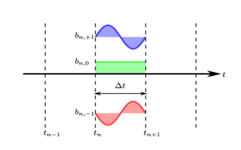
((a))

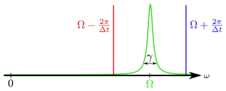
((b))

Figure 6: (a) On-resonance and first two sideband discrete temporal modes, represented in the interaction picture, where the on-resonance mode has frequency $\omega_{0}=\Omega$ ($\epsilon=0$) and the first two sideband modes have frequencies $\omega_{\pm}=\Omega\pm 2\pi/\Delta t$ ($\epsilon=\pm 2\pi/\Delta t$). (b) Illustration of the case where the interaction is sufficiently weak that the first two sideband discrete modes—and, hence, all the other sidebands—are sufficiently off resonance to ignore; it is thus also true that sensitivity to low frequencies is small enough that we can introduce the phantom negative-frequency field modes of Eq. 43, with frequencies $\omega=\Omega+\epsilon<0$, without altering the physics. This diagram illustrates the essential assumptions for the RWA and the quasimonochromatic approximation: $\gamma\ll 1/\Delta t\ll\Omega$.

Before exploring the interaction unitary, however, it is good to pause to review, expand, and formalize the assumptions necessary to get to the discrete Hamiltonian (52) that applies to each time segment or, more generally, to get to the Markovian quantum circuit of Fig. 4. The restriction of the system-probe interaction to be a sequence of joint unitaries between the system and a single probe segment is often referred to as the first Markov approximation. This approximation is valid when the spatial extent $\Delta x$ of the system is small with respect to the spatial extent $c\Delta t$ of the discretized probes. For many typical scenarios (e.g., atomic systems), the time interval $\Delta t$ can be made quite small, often even smaller than the characteristic evolution time $\Omega^{-1}$, before the spatial extent of the probes becomes comparable to the spatial extent of the system, which would force us to use a non-Markovian description like Fig. 5(b). The reason we did not encounter this assumption in the analysis above is that it is already incorporated in our starting point, the interaction Hamiltonian (38). A typical interaction Hamiltonian involves a spatial integral over the extent of the system. In writing the interaction Hamiltonian (38), we have already assumed that the system is small enough that the spatial integral can be replaced by a point interaction.

The initial product state of the probes is often referred to as the second Markov approximation. This approximation is valid when the correlation time $\tau_{c}$ in the bath is much shorter than the duration $\Delta t$ of the discrete probe segments. This is often an excellent approximation, as baths with even very low temperatures have very small correlation times. For example, the thermal correlation time $\tau_{c}=\hbar/2\pi kT\simeq 10\,{\rm ps}/T$ given by Eq. (3.3.20) in Gardiner and Zoller (2004) is approximately $10\,\mathrm{ns}$ for a temperature of $1\,\mathrm{mK}$. On the other hand, the vacuum correlation time $\tau_{c}\simeq 1/2\pi\Omega$ at the characteristic frequency means that if vacuum noise dominates, then the second Markov approximation requires that the probe segments be much longer than the system’s dynamical time, i.e., $\Delta t\gg 1/\Omega$. For a treatment of the nonzero correlation time of the vacuum in an exactly solvable model, see Unruh and Zurek (1989).

The product measurements at the output of the circuit in Fig. 4(c) do not affect open-system dynamics, for which the bath is not monitored, but they do enter into a Markovian description of dynamics conditioned on measurement of the bath. The product measurements are a good approximation when the bandwidth of the detectors is sufficiently wide to give temporal resolution much finer than the duration of the probe segments we used to discretize the bath.

The remaining pair of closely related approximations, as we discussed previously, are the RWA, which has to do with simplifying the form of the interaction Hamiltonian, and the quasimonochromatic approximation, which has to do with simplifying the description of the field so that each $\Delta t$ probe segment has only one relevant probe mode. The three important parameters in these two approximations are the characteristic system frequency $\Omega$, the linewidth $\gamma$, and the duration of the time segments, $\Delta t$, and the approximations require that $\gamma\ll 1/\Delta t\ll\Omega$.

The approximations we make are summarized below:

$$\Delta x\ll c\Delta t$$ First Markov, (53)

$$\tau_{c}\ll\Delta t$$ Second Markov, (54)

$$\Omega^{-1}\ll\Delta t\ll\gamma^{-1}$$ RWA and quasimonochromatic. (55)

We note that it is possible to model systems with several different, well-separated transition frequencies by introducing separate probe fields for each transition frequency, as long as it is possible to choose discrete probe time segments in such a way that the above approximations are valid for all fields introduced. The several probe fields can actually be parts of a single probe field, with each part consisting of the probe frequencies that are close to resonance with a particular transition frequency.

The approximations now well in hand, we return to the Hamiltonian (52) for the $n$th probe segment. The associated interaction unitary between the system and the $n$th probe segment is given by

$$U^{(n)}_{I}=e^{-iH^{(n)}_{I}\Delta t}=\mathds{1}\otimes\mathds{1}+\sqrt{\Delta\tau}\left(c\otimes b^{\dagger}_{n}-c^{\dagger}\otimes b_{n}\right)+\frac{1}{2}\Delta\tau\left(c\otimes b^{\dagger}_{n}-c^{\dagger}\otimes b_{n}\right)^{2}+\mathcal{O}\big{(}(\Delta\tau)^{3/2}\big{)}\,,$$ (56)

where we define a dimensionless time interval,

$$\Delta\tau \mathrel{\mathop{:}}=\gamma\Delta t\ll 1\,,$$ (57)

suitable for series expansions. We only need to expand the unitary to second order because we are only interested in terms up to order $\Delta\tau$ for writing first-order differential equations. A comprehensive and related presentation of the issues discussed above can be found in the recent paper of Fischer et al. (2017).

Notice that we can account for an external Hamiltonian $H_{\text{ext}}$ applied to the system, provided it changes slowly on the characteristic dynamical time scale $1/\Omega$ of the system and leads to slow evolution of the system on the characteristic time scale (if such a Hamiltonian is not slow, it should be included in the free system Hamiltonian $H_{\text{sys}}$). In the interaction picture, the external Hamiltonian acquires a time dependence and becomes part of the interaction Hamiltonian; since it is essentially constant in each time segment, its effect in each time segment can be captured by expanding its effect to linear order in $\Delta t$. It is easy to see that the interaction unitary (56) is then supplemented by an additional term $-i\Delta t\,H_{\text{ext}}$; when we convert to the final differential equation, this term introduces the standard commutator $-i\,dt\,[H_{\text{ext}},\rho]$ for an external Hamiltonian.

V Quantum trajectories for vacuum field and qubit probes

We are now prepared to discuss the quantum trajectories arising from the continuous measurement of a probe field coupled to a system as described in the previous section. In this context we often drop the explicit reference to which probe segment we are dealing with, since the Markovicity of Fig. 4(c) means we can consider each probe segment separately. Unconditional open-system evolution follows from averaging over the quantum trajectories or, equivalently, tracing out the probes.

Probe fields initially in the vacuum state are our concern in this section. Because the interaction between individual probes and the system is weak, the one-photon amplitude of the post-interaction probe segment is $\mathcal{O}(\sqrt{\!\Delta\tau}\,)$, the two-photon amplitude is $\mathcal{O}(\Delta\tau)$, and so on. Since these amplitudes are squared in probability calculations, the probability of detecting a probe with more than one photon is $\mathcal{O}(\Delta\tau^{2})$ and can be ignored. This suggests that it is sufficient to model the probe segments with qubits, with $\left|{g}\right\rangle$ corresponding to the vacuum state of the field and $\left|{e}\right\rangle$ corresponding to the single-photon state. We replace the discrete-field-mode annihilation operator $b_{n}$ in Eq. (56) with the qubit lowering operator $\sigma_{-}$ and $b_{n}^{\dagger}$ with $\sigma_{+}$:

$$U_{I} =\mathds{1}\otimes\mathds{1}+\sqrt{\!\Delta\tau}\,\left(c\otimes\sigma_{+}-c^{\dagger}\otimes\sigma_{-}\right)+\frac{1}{2}\Delta\tau\left(c\otimes\sigma_{+}-c^{\dagger}\otimes\sigma_{-}\right)^{2}$$ (58a)

$$=\mathds{1}\otimes\mathds{1}+\sqrt{\!\Delta\tau}\,\left(c\otimes\sigma_{+}-c^{\dagger}\otimes\sigma_{-}\right)-\frac{1}{2}\Delta\tau\left(c\,c^{\dagger}\otimes\left|{e}\middle\rangle\middle\langle{e}\right|+c^{\dagger}c\otimes\left|{g}\middle\rangle\middle\langle{g}\right|\right)\,.$$ (58b)

With this replacement, the neglect of two-photon transitions in the probe-field segments is made exact by the fact that $\sigma_{+}^{2}=\sigma_{-}^{2}=0$; these squared terms thus do not appear in Eq. (58b).

In Secs. V.1–V.4 we establish the correspondence between this qubit model and vacuum SMEs, where vacuum refers to the state of the probe field. In particular, we present qubit analogues of three typical measurements performed on probe fields: photon counting, homodyne measurement, and heterodyne measurement.

We transcend the vacuum probe fields in Sec. VI to Gaussian probe fields and find that formulating a qubit model requires additional tricks beyond just noting that weak interactions with the probe do not lead to significant two-photon transitions. Nevertheless, we are able to find qubit models that yield all the essential features of these Gaussian stochastic evolutions.

While the qubit model we develop is meant to capture the behavior of a “true” field-theoretic model, it is important to note that there are scenarios where qubits are the natural description. For example, in Haroche-style experiments Sayrin et al. (2011) a cavity interacts with a beam of atoms, accurately described as a sequence of finite-dimensional quantum probes. Such scenarios have been analyzed for their non-Markovian behavior (Scully and Zubairy, 1997, Sec. 9.2), and similar models are increasingly studied in the thermodynamics literature Horowitz (2012); Strasberg et al. (2017) and collisional models Giovannetti and Palma (2012); Rybár et al. (2012); Ciccarello (2017).

V.1 Z basis measurement: Photon counting or direct detection

As a first example, we consider performing photon-counting measurements on the probe field after its interaction with the system. We calculate the quantum trajectory by first constructing the Kraus operators given by Eq. 19. For probes initially in the vacuum state we have $\left|{\phi}\right\rangle=\left|{g}\right\rangle$, and our interaction unitary is given by Eqs. (58). What remains is to identify the measurement outcomes $\left\langle{o_{j}}\right|$. The qubit version of the number operator $b^{\dagger}b$ is $\sigma_{+}\sigma_{-}=\left|{e}\middle\rangle\middle\langle{e}\right|=\mbox{$\frac{1}{2}$}(\mathds{1}+\sigma_{z})$. Measuring this observable, as depicted in Fig. 7, is equivalent to measuring $\sigma_{z}$. The measurement outcomes are then $\left\langle{g}\right|$ and $\left\langle{e}\right|$ and give the Kraus operators

$$K_{g} =\left\langle{g}\middle|{U_{I}}\middle|{g}\right\rangle=\mathds{1}-\mbox{$\frac{1}{2}$}\Delta\tau\,c^{\dagger}c\,,$$ (59a)

$$K_{e} =\left\langle{e}\middle|{U_{I}}\middle|{g}\right\rangle=\sqrt{\!\Delta\tau}\,c\,.$$ (59b)

The corresponding POVM elements (to linear order in $\Delta\tau$) are

$$E_{g} =K_{g}^{\dagger}K_{g}=\mathds{1}-\Delta\tau\,c^{\dagger}c\,,$$ (60a)

$$E_{e} =K_{e}^{\dagger}K_{e}=\Delta\tau\,c^{\dagger}c\,,$$ (60b)

which trivially satisfy $E_{g}+E_{e}=\mathds{1}$. We call the Kraus operators (59) the photon-counting Kraus operators. These operators are identical to those derived for photon counting with continuous field modes (Wiseman and Milburn, 2010, Eqs. 4.5 and 4.7), as we expected from the vanishing multi-photon probability discussed earlier.

Figure 7: Circuit depicting the system interacting with a vacuum probe (probe initially in the ground state) which is subsequently subjected to measurement of the qubit number operator $\sigma_{+}\sigma_{-}$, the qubit analogue of a photon-counting measurement. The eigenvectors of $\sigma_{+}\sigma_{-}=\left|{e}\middle\rangle\middle\langle{e}\right|=\mbox{$\frac{1}{2}$}(\mathds{1}+\sigma_{z})$ are identical to those of $\sigma_{z}$, thus allowing us to think instead of a measurement of the Pauli observable $\sigma_{z}$.

To calculate a quantum trajectory we need to describe the evolution of the system conditioned on the outcomes of repeated measurements of this kind. The state of the system after making a measurement and getting the result $g$ during the $(n+1)$th time interval, i.e., between $t_{n}$ and $t_{n+1}$, is

$$\rho_{n+1|g}\mathrel{\mathop{:}}=\frac{K_{g}\rho_{n}K_{g}^{\dagger}}{\operatorname{Tr}\left[{{\rho_{n}E_{g}}}\right]}=\frac{\rho_{n}-\mbox{$\frac{1}{2}$}\Delta\tau\,\left(c^{\dagger}c\rho_{n}+\rho_{n}c^{\dagger}c\right)}{1-\Delta\tau\,\operatorname{Tr}\left[{{\rho_{n}c^{\dagger}c}}\right]}\,.$$ (61)

The subscript $n+1$ on $\rho_{n+1|g}$ indicates, as in Eq. (28), that this is the state at the end of this probe segment, after the measurement; the subscript $g$ indicates that this is the state conditioned on the measurement outcome $g$. The state $\rho_{n+1}$ is conditioned on all previous measurement outcomes as well, but we omit all of that conditioning, letting it be implicit in $\rho_{n}$. Expanding the denominator to first order in $\Delta\tau$ using the standard expansion $(1+x\Delta\tau)^{-1}=1-x\Delta\tau+\mathcal{O}(\Delta\tau^{2})$ allows us to calculate the difference equation (30) when the measurement result is $g$:

$$\begin{split}\Delta\rho_{n|g}&\mathrel{\mathop{:}}=\rho_{n+1|g}-\rho_{n}\\ &=-\mbox{$\frac{1}{2}$}\Delta\tau\,\Bigl{(}c^{\dagger}c\rho_{n}+\rho_{n}c^{\dagger}c-2\rho_{n}\operatorname{Tr}\left[{{\rho_{n}c^{\dagger}c}}\right]\Bigr{)}+\mathcal{O}(\Delta\tau^{2})\\ &=-\mbox{$\frac{1}{2}$}\Delta\tau\,\mathcal{H}\left[{c^{\dagger}c}\right]\rho_{n}\,,\end{split}$$ (62)

where we employ the shorthand

$$\mathcal{H}\left[{X}\right]\rho\mathrel{\mathop{:}}=X\rho+\rho X^{\dagger}-\rho\operatorname{Tr}\left[{{\rho(X+X^{\dagger})}}\right]\,.$$ (63)

Repeating the analysis for the case when the measurement result is $e$ gives

$$\rho_{n+1|e}\mathrel{\mathop{:}}=\frac{K_{e}\rho_{n}K_{e}^{\dagger}}{\operatorname{Tr}\left[{{\rho_{n}E_{e}}}\right]}=\frac{c\rho_{n}c^{\dagger}}{\operatorname{Tr}\left[{{\rho_{n}c^{\dagger}c}}\right]}\,.$$ (64)

The difference between the pre- and post-measurement system states when the measurement result is $e$ is thus

$$\Delta\rho_{n|e}\mathrel{\mathop{:}}=\rho_{n+1|e}-\rho_{n}=\frac{c\rho_{n}c^{\dagger}}{\operatorname{Tr}\left[{{\rho_{n}c^{\dagger}c}}\right]}-\rho_{n}=\mathcal{G}\left[{c}\right]\rho_{n}\,,$$ (65)

where we define

$$\mathcal{G}[X]\rho\mathrel{\mathop{:}}=\frac{X\rho X^{\dagger}}{\operatorname{Tr}\left[{{\rho X^{\dagger}X}}\right]}-\rho\,.$$ (66)

Having separate equations for the two measurement outcomes is not at all convenient. Fortunately, we can combine the equations by introducing a random variable $\Delta N$ that represents the outcome of the measurement:

$$\Delta N :g\mapsto 0\;,e\mapsto 1\,.$$ (67)

Since this random variable is a bit (i.e., a Bernoulli random variable) its statistics are completely specified by its mean:

$$\mathbb{E}\left[\Delta N\right]=0\cdot\operatorname{Tr}\left[{{\rho E_{g}}}\right]+1\cdot\operatorname{Tr}\left[{{\rho E_{e}}}\right]=\Delta\tau\,\operatorname{Tr}\left[{{\rho c^{\dagger}c}}\right].$$ (68)

We now combine the difference equations into a single stochastic equation using the random variable $\Delta N$:

$$\begin{split}\Delta\rho_{n|\Delta N}&\mathrel{\mathop{:}}=\rho_{n+1|\Delta N}-\rho_{n}\\ &=\Delta N\left(\frac{c\rho_{n}c^{\dagger}}{\operatorname{Tr}\left[{{\rho_{n}c^{\dagger}c}}\right]}-\rho_{n}\right)-(1-\Delta N)\mbox{$\frac{1}{2}$}\Delta\tau\,\Bigl{(}c^{\dagger}c\rho_{n}+\rho_{n}c^{\dagger}c-2\rho_{n}\operatorname{Tr}\left[{{\rho_{n}c^{\dagger}c}}\right]\Bigr{)}\\ &=\Delta N\mathcal{G}\left[{c}\right]\rho_{n}-(1-\Delta N)\mbox{$\frac{1}{2}$}\Delta\tau\,\mathcal{H}\left[{c^{\dagger}c}\right]\rho_{n}\,.\end{split}$$ (69)

It quickly becomes unnecessarily tedious to keep time-step indices around explicitly, since everything in our equations now refers to the same time step, so we drop those indices now. Discarding $\Delta N\Delta\tau$, since it is second-order in $\Delta\tau$ (see Eq. (68) and (Wiseman and Milburn, 2010, Chap. 4)), we simplify Eq. (69) to

$$\begin{split}\Delta\rho_{\Delta N}&=\Delta N\left(\frac{c\rho c^{\dagger}}{\operatorname{Tr}\left[{{\rho c^{\dagger}c}}\right]}-\rho\right)-\mbox{$\frac{1}{2}$}\Delta\tau\,\Bigl{(}c^{\dagger}c\rho+\rho c^{\dagger}c-2\rho\operatorname{Tr}\left[{{\rho c^{\dagger}c}}\right]\Bigr{)}\\ &=\Delta\tau\,\mathcal{D}[c]\rho+\Delta\mathcal{I}_{D}\mathcal{G}\left[{c}\right]\rho\,,\end{split}$$ (70)

where we introduce the standard diffusion superoperator,

$$\mathcal{D}[X]\rho\mathrel{\mathop{:}}=X\rho X^{\dagger}-\mbox{$\frac{1}{2}$}(X^{\dagger}X\rho+\rho X^{\dagger}X)\,,$$ (71)

and the photon-counting innovation,

$$\Delta\mathcal{I}_{D}\mathrel{\mathop{:}}=\Delta N-\mathbb{E}\left[\Delta N\right]\,,$$ (72)

which is the difference between the measurement result and the mean result (i.e., it can be thought of as what is learned from the measurement). The subscript $D$ here plays off the fact that photon counting is often called direct detection and is used in place of $N$ because $N$ has too many other uses in this paper.

By taking the limit $\Delta\tau\to\gamma dt$ we obtain a stochastic differential equation,

$$\begin{split}d\rho_{D}&=dN\left(\frac{c\rho c^{\dagger}}{\operatorname{Tr}\left[{{\rho c^{\dagger}c}}\right]}-\rho\right)-\mbox{$\frac{1}{2}$}\gamma dt\,\Bigl{(}c^{\dagger}c\rho+\rho c^{\dagger}c-2\rho\operatorname{Tr}\left[{{\rho c^{\dagger}c}}\right]\Bigr{)}\\ &=dt\,\mathcal{D}[\sqrt{\gamma}\,c]\rho+d\mathcal{I}_{D}\mathcal{G}\left[{c}\right]\rho\,,\end{split}$$ (73)

where $dN$ is a bit-valued random process, termed a point process, with mean $\mathbb{E}\left[dN\right]=\gamma dt\,\operatorname{Tr}\left[{{\rho c^{\dagger}c}}\right]$ and the innovation is given by $d\mathcal{I}_{D}=dN-\mathbb{E}\left[dN\right]$. This equation is called the vacuum stochastic master equation (SME) for photon counting; i.e., it is the stochastic differential equation that describes the conditional evolution of a system that interacts with vacuum probes that are subjected to photon-counting measurements.

Equation 73 has no explicit system-Hamiltonian term. Although this differs from other presentations our readers might be familiar with, it is merely an aesthetic distinction. Recall from the discussion at the end of Section IV that well-behaved system Hamiltonians can be introduced by including an additional commutator term in our differential equations. In this case, the modification yields

$$\begin{split}d\rho_{D}&=-i\,dt\,[H_{\text{ext}},\rho]+dt\,\mathcal{D}[\sqrt{\gamma}\,c]\rho+d\mathcal{I}_{D}\mathcal{G}\left[{c}\right]\rho\,.\end{split}$$ (74)

It is important to stress that in practice, for numerical integration of these equations, one uses the difference equation (70), not the differential equation (73); i.e., what one uses in practice is the difference equation that corresponds to the discrete-time quantum circuit in Fig. 4(c). One assigns to the system a prior state $\rho_{0}$ that combines with the initial probe states to make an initial product state on the full system/probe arrangement. This prior state describes the system at the moment coupling to the probes is turned on and measurements begin. Each time a new measurement result is sampled, Eq. 70 is used to update the description of the system. If we describe our system by $\rho_{n}$ after collecting $n$ samples from our measurement device, observing $\Delta N$ for sample $n+1$ leads to the updated state $\rho_{n+1}=\rho_{n}+\Delta\rho_{\Delta N}$.

Another application of the difference equation is state/parameter inference. In the case of state inference, one has uncertainty regarding what initial state $\rho_{0}$ to assign to the system. General choices for $\rho_{0}$ will be incorrect, invalidating some of the properties described above. In particular, the innovation will deviate from a zero-mean random variable, and these deviations observed for a variety of guesses for $\rho_{0}$ will yield likelihood ratios that can be used to estimate the state, as was done in Cook et al. (2014). One can also keep track of the trace of the unnormalized state (23), which encodes the relative likelihood of the trajectory given the evolution parameters, allowing one to judge different parameter values against one another, as was implemented in Chase and Geremia (2009).

The differential equation that describes the unconditional evolution corresponding to Eq. (73) is called the master equation. To obtain the master equation, we simply average over measurement results in Eq. 73. The only term that depends on the results is $d\mathcal{I}_{D}$, and its mean is zero, so the master equation is

$$d\rho=\mathbb{E}\left[d\rho_{D}\right]=dt\,\mathcal{D}\left[{\sqrt{\gamma}\,c}\right]\rho\,.$$ (75)

Just as was the case for the SME (73), Eq. 75 has no explicit system-Hamiltonian term. The same reasoning that allowed us to add such a term and arrive at Eq. 74 allows us to add the same term to Eq. 75:

$$d\rho=\mathbb{E}\left[d\rho_{D}\right]=-i\,dt\,[H_{\text{ext}},\rho]+dt\,\mathcal{D}\left[{\sqrt{\gamma}\,c}\right]\rho\,.$$ (76)

For the remainder of our presentation, such system-Hamiltonian terms are generally left implicit.

V.2 X basis measurement: Homodyne detection

We can produce, as in Brun’s model Brun (2002), a different system evolution simply by measuring the probes in a different basis. To be concrete, let us consider measuring the $x$-quadrature of the field, $b^{\dagger}+b$. In the qubit-probe approach, this means measuring $\sigma_{+}+\sigma_{-}=\sigma_{x}$ as shown in Fig. 8.

Figure 8: Circuit depicting the system interacting with a vacuum probe (probe initially in the ground state) which is subsequently subjected to measurement of the qubit quadrature operator $\sigma_{+}+\sigma_{-}=\sigma_{x}$, the qubit analogue of a homodyne measurement. Just as for photon counting, the qubit measurement corresponds to a Pauli observable.

This measurement projects onto the eigenstates

$$\left|{\phi_{\pm}}\right\rangle\mathrel{\mathop{:}}=(\left|{g}\right\rangle\pm\left|{e}\right\rangle)/\sqrt{2}$$ (77)

of $\sigma_{x}$. The Kraus operators are linear combinations of the photon-counting Kraus operators,

$$K_{\pm} =\left\langle{\phi_{\pm}}\middle|{U_{I}}\middle|{g}\right\rangle=\frac{1}{\sqrt{2}}\left(K_{g}\pm K_{e}\right)=\frac{1}{\sqrt{2}}\left(\mathds{1}\pm\sqrt{\!\Delta\tau}\,c-\mbox{$\frac{1}{2}$}\Delta\tau\,c^{\dagger}c\right)\,,$$ (78)

and the corresponding POVM elements (to linear order in $\Delta\tau$) are

$$E_{\pm}=K^{\dagger}_{\pm}K_{\pm}=\frac{1}{2}\Big{(}\mathds{1}\pm\sqrt{\!\Delta\tau}\,(c+c^{\dagger})\Big{)}\,,$$ (79)

which clearly satisfy $E_{+}+E_{-}=\mathds{1}$. We write the difference equation as before, keeping terms up to order $\Delta\tau$,

$$\begin{split}\Delta\rho_{\pm}&\mathrel{\mathop{:}}=\frac{K_{\pm}\rho K_{\pm}^{\dagger}}{\operatorname{Tr}\left[{{\rho E_{\pm}}}\right]}-\rho\\ &=\frac{\rho\pm\sqrt{\!\Delta\tau}\,(c\rho+\rho c^{\dagger})+\Delta\tau\,\mathcal{D}\left[{c}\right]\rho}{1\pm\sqrt{\!\Delta\tau}\,\operatorname{Tr}\left[{{\rho(c+c^{\dagger})}}\right])}-\rho\\ &=\left(\pm\sqrt{\!\Delta\tau}\,-\Delta\tau\,\operatorname{Tr}\left[{{(c+c^{\dagger})\rho}}\right]\right)\mathcal{H}\left[{c}\right]\rho+\Delta\tau\,\mathcal{D}\left[{c}\right]\rho\,,\end{split}$$ (80)

where we have again expanded the denominator using a standard series,

$$\frac{1}{1+x\sqrt{\!\Delta\tau}\,} =1-x\sqrt{\!\Delta\tau}\,+x^{2}\Delta\tau+\mathcal{O}(\Delta\tau^{3/2})\,.$$ (81)

The dependence on the measurement result $\pm$ is reduced now to the coefficient $\pm\sqrt{\!\Delta\tau}\,$ in Eq. 80. We rewrite this stochastic coefficient as a random variable, $\Delta R$, again dependent on the measurement outcome such that ${\Delta R:\pm\mapsto\pm\sqrt{\!\Delta\tau}\,}$. The average of this random variable to order $\Delta\tau$ is

$$\mathbb{E}\left[\Delta R\right]=\sqrt{\!\Delta\tau}\,\operatorname{Tr}\left[{{\rho E_{+}}}\right]-\sqrt{\!\Delta\tau}\,\operatorname{Tr}\left[{{\rho E_{-}}}\right]=\Delta\tau\,\operatorname{Tr}\left[{{(c+c^{\dagger})\rho}}\right]\,.$$ (82)

This is exactly the term subtracted from $\Delta R$ in the coefficient of $\mathcal{H}\left[{c}\right]\rho$ in Eq. 80; thus, defining the homodyne version of the innovation as

$$\Delta\mathcal{I}_{H}\mathrel{\mathop{:}}=\Delta R-\mathbb{E}\left[\Delta R\right]\,,$$ (83)

we bring the homodyne difference equation into the form,

$$\Delta\rho_{\pm}=\Delta\tau\,\mathcal{D}\left[{c}\right]\rho+\Delta\mathcal{I}_{H}\mathcal{H}\left[{c}\right]\rho\,,$$ (84)

which is the difference equation one uses for numerical integration in the presence of homodyne measurements.

Another simple calculation shows the second moment of $\Delta R$ to be

$$\mathbb{E}\left[(\Delta R)^{2}\right]=\Delta\tau\,\operatorname{Tr}\left[{{E_{+}\rho}}\right]+\Delta\tau\,\operatorname{Tr}\left[{{E_{-}\rho}}\right]=\Delta\tau\,.$$ (85)

By definition the innovation has zero mean, and its second moment is the variance of $\Delta R$,

$$\mathbb{E}\left[(\Delta\mathcal{I}_{H})^{2}\right]=\mathbb{E}\left[(\Delta R)^{2}\right]-(\mathbb{E}\left[\Delta R\right])^{2}=\Delta\tau\,,$$ (86)

where again we work to linear order in $\Delta\tau$. It is now trivial to write the continuous-time stochastic differential equation that goes with the difference equation (84):

$$d\rho_{H} =dt\,\mathcal{D}\left[{\sqrt{\gamma}\,c}\right]\rho+dW\,\mathcal{H}\left[{\sqrt{\gamma}\,c}\right]\rho\,.$$ (87)

In the continuous limit, the innovation $\Delta\mathcal{I}_{H}$ becomes $\sqrt{\gamma}\,dW$, where $dW$ is the Weiner process, satisfying $\mathbb{E}\left[dW\right]=0$ and $\mathbb{E}\left[dW^{2}\right]=dt$.

Changing the measurement performed on the probes does not alter the unconditional evolution of the system, so averaging over the homodyne measurement results gives again the master equation (75):

$$d\rho=\mathbb{E}\left[d\rho_{H}\right]=dt\,\mathcal{D}\left[{\sqrt{\gamma}\,c}\right]\rho=\mathbb{E}\left[d\rho_{D}\right]\,.$$ (88)

The results so far in this subsection are for homodyne detection of the probe quadrature component $X=\sigma_{+}+\sigma_{-}=\sigma_{x}$, i.e., measurement in the basis (77). It is easy to generalize to measurement of an arbitrary field quadrature $e^{i\varphi}b+e^{-i\varphi}b^{\dagger}$, which for a qubit probe becomes a measurement of the spin component

$$X(\varphi)\mathrel{\mathop{:}}=e^{i\varphi}\sigma_{-}+e^{-i\varphi}\sigma_{+}=\sigma_{x}\cos\varphi+\sigma_{y}\sin\varphi\,.$$ (89)

This means measurement in the probe basis [eigenstates of $X(\varphi)$],

$$\left|{\phi_{\pm}(\varphi)}\right\rangle\mathrel{\mathop{:}}=\frac{1}{\sqrt{2}}\big{(}\left|{g}\right\rangle\pm e^{-i\varphi}\left|{e}\right\rangle\big{)}\,,$$ (90)

where we can also write

$$\begin{split}\left|{\phi_{+}(\varphi)}\right\rangle&=e^{-i\varphi/2}\big{[}\cos(\varphi/2)\left|{\phi_{+}}\right\rangle+i\sin(\varphi/2)\left|{\phi_{-}}\right\rangle\big{]}\,,\\ \left|{\phi_{-}(\varphi)}\right\rangle&=e^{-i\varphi/2}\big{[}i\sin(\varphi/2)\left|{\phi_{+}}\right\rangle+\cos(\varphi/2)\left|{\phi_{-}}\right\rangle\big{]}\,.\end{split}$$ (91)

The resulting Kraus operators are

$$\begin{split}K_{\pm}(\varphi)&=\left\langle{\phi_{\pm}(\varphi)}\middle|{U_{I}}\middle|{g}\right\rangle\\ &=\frac{1}{\sqrt{2}}\big{(}K_{g}\pm e^{i\varphi}K_{e}\big{)}\\ &=\frac{1}{\sqrt{2}}\Big{(}\mathds{1}\pm\sqrt{\!\Delta\tau}\,e^{i\varphi}c-\mbox{$\frac{1}{2}$}\Delta\tau\,c^{\dagger}c\Big{)}\,,\end{split}$$ (92)

with corresponding POVM elements

$$E_{\pm}(\varphi)=K_{\pm}^{\dagger}(\varphi)K_{\pm}(\varphi)=\frac{1}{2}\Big{(}\mathds{1}\pm\sqrt{\!\Delta\tau}\,(e^{i\varphi}c+e^{-i\varphi}c^{\dagger})\Big{)}\,.$$ (93)

We see that the results for measuring $X$ can be converted to those for measuring $X(\varphi)$ by replacing $c$ with $c\,e^{i\varphi}$. Thus the conditional difference equation is

$$\Delta\rho_{\pm}=\Delta\tau\,\mathcal{D}\left[{c}\right]\rho+\Delta\mathcal{I}_{H}\mathcal{H}\left[{c\,e^{i\varphi}}\right]\rho\,,$$ (94)

and the vacuum SME becomes

$$d\rho_{H} =dt\,\mathcal{D}\left[{\sqrt{\gamma}\,c}\right]\rho+dW\,\mathcal{H}\left[{\sqrt{\gamma}\,c\,e^{i\varphi}}\right]\rho\,.$$ (95)

V.3 Generalized measurement of X and Y: Heterodyne detection

Heterodyne measurement can be thought of as simultaneous measurement of two orthogonal field quadrature components, e.g., $b+b^{\dagger}$ and $-i(b-b^{\dagger})$. In our qubit model, this corresponds to simultaneously measuring along two orthogonal axes in the $x$-$y$ plane of the Bloch sphere, e.g., $\sigma_{-}+\sigma_{+}=\sigma_{x}=X$ and $i(\sigma_{-}-\sigma_{+})=\sigma_{y}=Y=X(\pi/2)$. Obviously, it is not possible to measure these two qubit observables simultaneously and perfectly, since they do not commute, but we can borrow a strategy employed in optical experiments to measure two quadrature components simultaneously. The optical strategy makes two “copies” of the field mode to be measured, by combining the field mode with vacuum at a 50-50 beamsplitter; this is followed by orthogonal homodyne measurements on the two copies. This strategy works equally well for our qubit probes, once we define an appropriate beamsplitter unitary for two qubits,

$$\begin{split}\mathrm{BS}(\eta)&\mathrel{\mathop{:}}=\exp\Big{[}i\big{(}\eta\sigma_{-}\otimes\sigma_{+}+\eta^{*}\sigma_{+}\otimes\sigma_{-}\big{)}\Big{]}\\ &=\left|{gg}\middle\rangle\middle\langle{gg}\right|+\left|{ee}\middle\rangle\middle\langle{ee}\right|+\cos|\eta|\,\big{(}\left|{ge}\middle\rangle\middle\langle{ge}\right|+\left|{eg}\middle\rangle\middle\langle{eg}\right|\big{)}+i\sin|\eta|\,\big{(}e^{i\delta}\left|{ge}\middle\rangle\middle\langle{eg}\right|+e^{-i\delta}\left|{eg}\middle\rangle\middle\langle{ge}\right|\big{)}\,,\end{split}$$ (96)

where $\eta=|\eta|e^{i\delta}$. Specializing to $\eta=-i\pi/4$ yields

$$\mathrm{BS}\mathrel{\mathop{:}}=\mathrm{BS}(-i\pi/4)=\left|{gg}\middle\rangle\middle\langle{gg}\right|+\left|{ee}\middle\rangle\middle\langle{ee}\right|+\frac{1}{\sqrt{2}}\big{(}\left|{ge}\middle\rangle\middle\langle{ge}\right|+\left|{eg}\middle\rangle\middle\langle{eg}\right|+\left|{ge}\middle\rangle\middle\langle{eg}\right|-\left|{eg}\middle\rangle\middle\langle{ge}\right|\big{)}\,.$$ (97)

This “beamsplitter” behaves rather strangely when excitations are fed to both input ports, but this isn’t an issue since the second (top) port of the beamsplitter is fed the ground state, as illustrated in Fig. 9.

Figure 9: Beamsplitter implementation of heterodyne measurement of $x$ and $y$ spin components of a qubit probe.

It is useful to note here, for use a bit further on, that the beamsplitter unitary, when written in terms of Pauli operators, factors into two commuting unitaries,

$$\mathrm{BS}=\exp\bigg{(}i\frac{\pi}{8}\sigma_{x}\otimes\sigma_{y}\bigg{)}\exp\bigg{(}\!-i\frac{\pi}{8}\sigma_{y}\otimes\sigma_{x}\bigg{)}\,.$$ (98)

This factored form is easy to work with and leads to

$$\begin{split}\mathrm{BS}&=\Big{[}\mathds{1}\otimes\mathds{1}\cos(\pi/8)+i\sigma_{x}\otimes\sigma_{y}\sin(\pi/8)\Big{]}\Big{[}\mathds{1}\otimes\mathds{1}\cos(\pi/8)-i\sigma_{y}\otimes\sigma_{x}\sin(\pi/8)\Big{]}\\ &=\frac{1}{2}\big{(}\mathds{1}\otimes\mathds{1}+\sigma_{z}\otimes\sigma_{z}\big{)}+\frac{1}{2\sqrt{2}}\big{(}\mathds{1}\otimes\mathds{1}-\sigma_{z}\otimes\sigma_{z}+i\sigma_{x}\otimes\sigma_{y}-i\sigma_{y}\otimes\sigma_{x}\big{)}\,,\end{split}$$ (99)

which immediately confirms Eq. 97.

To calculate the Kraus operators for heterodyne measurement, we project the first probe qubit onto the eigenstates of the spin component $X=\sigma_{x}$ and second probe qubit onto the eigenstates of the spin component $Y=\sigma_{y}$. Before proceeding to that, we deal with a notational point for the eigenstates of $\sigma_{y}=Y=X(\pi/2)$, analogous to the notational convention for $\sigma_{x}$ that is summarized in Fig. 1. The conventional quantum-information notation for the $\pm 1$ eigenstates of $\sigma_{y}$ is $\left|{\pm i}\right\rangle=(\left|{0}\right\rangle\pm i\left|{1}\right\rangle)/\sqrt{2}$, whereas as we introduced in Eq. (90), we are using eigenstates that differ by a phase factor of $\mp i$:

$$\left|{\phi_{\pm i}}\right\rangle\mathrel{\mathop{:}}=\left|{\phi_{\pm}(\pi/2)}\right\rangle=\frac{1}{\sqrt{2}}\big{(}\left|{g}\right\rangle\mp i\left|{e}\right\rangle\big{)}=\mp i\frac{1}{\sqrt{2}}\big{(}\left|{0}\right\rangle\pm i\left|{1}\right\rangle\big{)}=\mp i\left|{\pm i}\right\rangle\,.$$ (100)

When all this is accounted for, the Kraus operators come out to be

$$\begin{split}K_{\pm,\mathbin{\widetilde{\pm}}}&=(\left\langle{\phi_{\pm}}\right|\otimes\left\langle{\phi_{\,\mathbin{\widetilde{\pm}}\,i}}\right|)(\mathds{1}\otimes\mathrm{BS})(U_{I}\otimes\mathds{1})\left|{gg}\right\rangle\\ &=\frac{1}{\sqrt{2}}\big{\langle}\phi_{\pm}(\pm\mathbin{\widetilde{\pm}}\pi/4)\big{|}U_{I}\big{|}g\big{\rangle}\\ &=\frac{1}{2}\big{(}K_{g}\pm e^{\pm\mathbin{\widetilde{\pm}}i\pi/4}K_{e}\big{)}\\ &=\frac{1}{2}\left(\mathds{1}\pm e^{\pm\mathbin{\widetilde{\pm}}i\pi/4}\sqrt{\Delta\tau}c-\frac{1}{2}\Delta\tau\,c^{\dagger}c\right)\,,\end{split}$$ (101)

where we have introduced two binary variables, $\pm$ and $\tilde{\pm}$, to account for the four measurement outcomes. The juxtaposition of these two variables, $\pm\mathbin{\widetilde{\pm}}$, denotes their product, i.e., the parity of the two bits. We see this notation at work in

$$\pm e^{\pm\mathbin{\widetilde{\pm}}i\pi/4}=\pm\frac{1}{\sqrt{2}}(1\,{\pm\mathbin{\widetilde{\pm}}}\,i)=\frac{1}{\sqrt{2}}(\pm 1\mathbin{\widetilde{\pm}}i)\,.$$ (102)

The POVM elements that correspond to the Kraus operators (101) are

$$E_{\pm,\mathbin{\widetilde{\pm}}} =\frac{1}{4}\left(\mathds{1}\pm\sqrt{\!\Delta\tau}\,\big{(}e^{\mp\mathbin{\widetilde{\pm}}i\pi/4}c^{\dagger}+e^{\pm\mathbin{\widetilde{\pm}}i\pi/4}c\big{)}\right)$$ (103)

$$=\frac{1}{4}\left[\mathds{1}+\sqrt{\!\Delta\tau}\,\left(\pm\frac{c+c^{\dagger}}{\sqrt{2}}\mathbin{\widetilde{\pm}}\frac{i(c-c^{\dagger})}{\sqrt{2}}\right)\right]\,.$$ (104)

The second form of the Kraus operators in Eq. 101 is equivalent to finding the Kraus operators of the primary probe qubit for the heterodyne measurement model on the left side of Fig. 9. One sees from this second form that the $\sigma_{x}$ and $\sigma_{y}$ measurements on the two probe qubits are equivalent to projecting the primary probe qubit onto one of the following four states:

$$\left|{\phi_{\pm,\mathbin{\widetilde{\pm}}}}\right\rangle\mathrel{\mathop{:}}=\left|{\phi_{\pm}(\pm\mathbin{\widetilde{\pm}}\pi/4)}\right\rangle=\frac{1}{\sqrt{2}}\left(\left|{g}\right\rangle\pm e^{\mp\mathbin{\widetilde{\pm}}i\pi/4}\left|{e}\right\rangle\right)=\frac{1}{\sqrt{2}}\left(\left|{g}\right\rangle+\frac{1}{\sqrt{2}}(\pm 1\mathbin{\widetilde{\mp}}i)\left|{e}\right\rangle\right)\,.$$ (105)

These four states are depicted in Fig. 10; they carry two bits of information, which are the results of the $\sigma_{x}$ and $\sigma_{y}$ measurements in the beamsplitter measurement model. The four states not being orthogonal, they must be subnormalized by the factor of $\sqrt{2}$ that appears in Eq. 101 to obtain legitimate Kraus operators.

Figure 10: The four states, $\left|{\phi_{\pm,\mathbin{\widetilde{\pm}}}}\right\rangle=\left|{\phi_{\pm}(\pm\mathbin{\widetilde{\pm}}\pi/4)}\right\rangle$, whose scaled projectors on the primary probe qubit make up the heterodyne POVM, as viewed in the $x$-$y$ plane of the Bloch sphere, shown relative to the positive and negative eigenstates of $\sigma_{x}=X$ and $\sigma_{y}=Y$.

We conclude that as far as the primary probe qubit is concerned, the heterodyne measurement can be regarded as flipping a fair coin to determine whether one measures $X(\pi/4)=(\sigma_{x}+\sigma_{y})/\sqrt{2}$ or $X(-\pi/4)=(\sigma_{x}-\sigma_{y})/\sqrt{2}$. The $\pm 1$ eigenstates of $X(\pi/4)$ are $\left|{\phi_{\pm}(\pi/4)}\right\rangle$; $\left|{\phi_{+}(\pi/4)}\right\rangle=\left|{\phi_{+\widetilde{+}}}\right\rangle$ has eigenvalue $+1$, and $\left|{\phi_{-}(\pi/4)}\right\rangle=\left|{\phi_{-\widetilde{-}}}\right\rangle$ has eigenvalue $-1$. The $\pm 1$ eigenstates of $X(-\pi/4)$ are $\left|{\phi_{\pm}(-\pi/4)}\right\rangle$; $\left|{\phi_{+}(-\pi/4)}\right\rangle=\left|{\phi_{+\widetilde{-}}}\right\rangle$ has eigenvalue $+1$, and $\left|{\phi_{-}(-\pi/4)}\right\rangle=\left|{\phi_{-\widetilde{+}}}\right\rangle$ has eigenvalue $-1$. Notice that the fair coin that decides between these two measurements is the parity of the measurements of $\sigma_{x}$ and $\sigma_{y}$ in the heterodyne circuit of Fig. 9. Figure 11 goes through the circuit identities that convert the heterodyne circuit involving measurements on two probe qubits to one that is a coin flip that chooses between the two measurement bases on the primary probe qubit.

Figure 11: Circuit-identity conversion of the original heterodyne measurement circuit of Fig. 9, which involves a beamsplitter on two probe qubits followed by $\sigma_{x}$ and $\sigma_{y}$ measurements on the two qubits, to a fair-coin flip, mediated by the ancillary (top) probe qubit, that chooses between measurements of $X(\varphi/4)$ and $X(-\varphi/4)$ on the primary (bottom) probe qubit. The first step writes the beamsplitter unitary $\mathrm{BS}$ as a product of the two commuting unitaries in Eq. 98. The second step makes major changes. It first discards the second piece of the beamsplitter unitary because that piece commutes with the measurements and thus has no effect on outcome probabilities. It then changes the initial state of the ancillary probe qubit to $\left|{e}\right\rangle$ by including a bit flip $\sigma_{x}$; surrounds the beamsplitter unitary on the top wire with $\pi/2$ rotations about $z$ at the expense of changing the top-wire $\sigma_{x}$ in the beamsplitter unitary to $-\sigma_{y}$, i.e., $\sigma_{x}=-R_{z}(\pi/2)\sigma_{y}R_{z}^{\dagger}(\pi/2)$; and finally, surrounds the beamsplitter unitary with Hadamard gates, $H=(\sigma_{x}+\sigma_{z})/\sqrt{2}$, on both wires, without changing the beamsplitter unitary because $H\sigma_{y}H=-\sigma_{y}$. The third step discards the first $z$ rotation on the top wire because it only introduces an irrelevant phase change; pushes the $\sigma_{x}$ on the top wire to the end of the circuit, with the sign of the second $\sigma_{y}$ in the beamsplitter unitary changing along the way and with the gate ultimately being discarded because it becomes a $\sigma_{y}$ gate preceding the $\sigma_{y}$ measurement; converts the measurements to $\sigma_{z}$ measurements by using $\sigma_{z}=H\sigma_{x}H=HR_{z}^{\dagger}(\pi/2)\sigma_{y}R_{z}(\pi/2)H$; and finally introduces an initial CNOT gate, which does nothing since it acts on the initial state $\left|{e}\right\rangle$ on the top wire. The fourth step pushes the CNOT through to the end of the circuit: the two Hadamards reverse the direction of the CNOT, putting the control on the bottom wire and the target on the top wire; pushing this CNOT through the beamsplitter unitary transforms the $\sigma_{y}\otimes\sigma_{y}$ to $-\sigma_{x}\otimes\sigma_{z}$. After this move, the bottom Hadamard is pushed through the beamsplitter unitary, further converting the $\sigma_{x}\otimes\sigma_{z}$ to $\sigma_{z}\otimes\sigma_{z}$. The fifth step converts the beamsplitter unitary to a rotation and a controlled rotation using $e^{i\sigma_{z}\otimes\sigma_{z}\pi/8}=\exp[-i\sigma_{z}\otimes\frac{1}{2}(\mathds{1}-\sigma_{z})\pi/4]e^{i\sigma_{z}\otimes\mathds{1}\pi/8}$; pushes the CNOT through the $\sigma_{z}$ measurements to become a classical controlled operation that does nothing if the outcome of the bottom measurement is the eigenvalue $+1$ ($\left|{e}\right\rangle$) and multiplies the result of the top measurement by $-1$ if the outcome of the bottom measurement is the eigenvalue $-1$ ($\left|{g}\right\rangle$); and finally pushes the Hadamard on the bottom wire through the measurement, converting it to a measurement of $\sigma_{x}$. The sixth step converts the controlled rotation into a classically controlled rotation of the bottom qubit, controlled on the outcome of the $\sigma_{z}$ measurement on the top qubit; this final circuit embodies the fair-coin flip version of the heterodyne measurement. The apparently irrelevant CNOT introduced in the third step is actually crucial. When pushed to the end of the circuit, it makes the outcome of the coin flip the parity of the original measurements of $\sigma_{x}$ and $\sigma_{y}$; the parity thus chooses between the measurement of $X(\pi/4)$ and $X(-\pi/4)$ on the primary probe qubit. The classical version of this CNOT at the end of the circuit is there to get strict equivalence to the original circuit; it returns the classical bit carried by the top wire to the outcome of the $\sigma_{y}$ measurement in the original circuit.

We now turn to deriving the explicit form of the conditional heterodyne difference equation,

$$\Delta\rho_{\pm,\mathbin{\widetilde{\pm}}} \mathrel{\mathop{:}}=\frac{K_{\pm,\mathbin{\widetilde{\pm}}}\,\rho\,K_{\pm,\mathbin{\widetilde{\pm}}}^{\dagger}}{\operatorname{Tr}\left[{{\rho E_{\pm,\mathbin{\widetilde{\pm}}}}}\right]}-\rho\,.$$ (106)

This time we need two binary random variables to account for the dependence on measurement outcome:

$$\Delta R_{x}:(\pm,\mathbin{\widetilde{\pm}})\mapsto\pm\sqrt{\!\Delta\tau}\,\,,$$ (107)

$$\Delta R_{y}:(\pm,\mathbin{\widetilde{\pm}})\mapsto\mathbin{\widetilde{\pm}}\sqrt{\!\Delta\tau}\,\,.$$ (108)

We want to write the equation in terms of innovations again, so we need the probability distribution of measurement outcomes in order to calculate $\mathbb{E}\left[\Delta R_{x}\right]$ and $\mathbb{E}\left[\Delta R_{y}\right]$:

$$\Pr(\pm,\mathbin{\widetilde{\pm}})=\operatorname{Tr}\left[{{\rho E_{\pm,\mathbin{\widetilde{\pm}}}}}\right]=\frac{1}{4}\Bigg{(}1\pm\sqrt{\!\Delta\tau}\,\operatorname{Tr}\left[{{\rho\frac{c+c^{\dagger}}{\sqrt{2}}}}\right]\mathbin{\widetilde{\pm}}\sqrt{\!\Delta\tau}\,\operatorname{Tr}\left[{{\rho\frac{ic+(ic)^{\dagger}}{\sqrt{2}}}}\right]\Bigg{)}\,.$$ (109)

The marginal probabilities, given by

$$\Pr(\pm) =\sum_{\mathbin{\widetilde{\pm}}}\Pr(\pm,\mathbin{\widetilde{\pm}})=\frac{1}{2}\Bigg{(}1\pm\sqrt{\!\Delta\tau}\,\operatorname{Tr}\left[{{\rho\frac{c+c^{\dagger}}{\sqrt{2}}}}\right]\Bigg{)}\,,$$ (110)

$$\Pr(\mathbin{\widetilde{\pm}}) =\sum_{\pm}\Pr(\pm,\mathbin{\widetilde{\pm}})=\frac{1}{2}\Bigg{(}1\mathbin{\widetilde{\pm}}\sqrt{\!\Delta\tau}\,\operatorname{Tr}\left[{{\rho\frac{ic+(ic)^{\dagger}}{\sqrt{2}}}}\right]\Bigg{)}\,,$$ (111)

allow us to calculate expectation values,

$$\mathbb{E}\left[\Delta R_{x}\right] =\sum_{\pm}\pm\sqrt{\!\Delta\tau}\,\Pr(\pm)=\Delta\tau\operatorname{Tr}\left[{{\rho\frac{c+c^{\dagger}}{\sqrt{2}}}}\right]\,,$$ (112)

$$\mathbb{E}\left[\Delta R_{y}\right] =\sum_{\mathbin{\widetilde{\pm}}}\mathbin{\widetilde{\pm}}\sqrt{\!\Delta\tau}\,\Pr(\mathbin{\widetilde{\pm}})=\Delta\tau\operatorname{Tr}\left[{{\rho\frac{ic+(ic)^{\dagger}}{\sqrt{2}}}}\right]\,.$$ (113)

We can also find the correlation matrix,

$$\mathbb{E}\left[(\Delta R_{x})^{2}\right] =\sum_{\pm}\Delta\tau\Pr(\pm)=\Delta\tau\,,$$ (114)

$$\mathbb{E}\left[(\Delta R_{y})^{2}\right] =\sum_{\mathbin{\widetilde{\pm}}}\Delta\tau\Pr(\mathbin{\widetilde{\pm}})=\Delta\tau\,,$$ (115)

$$\mathbb{E}\left[\Delta R_{x}\Delta R_{y}\right] =\sum_{\pm,\mathbin{\widetilde{\pm}}}\pm\mathbin{\widetilde{\pm}}\Delta\tau\Pr(\pm,\mathbin{\widetilde{\pm}})=0\,.$$ (116)

The first nonvanishing cross-moment of $\Delta R_{x}$ and $\Delta R_{y}$ is $\mathbb{E}\left[(\Delta R_{x})^{2}(\Delta R_{y})^{2}\right]=\Delta\tau^{2}$. This means that we should think of $\Delta R_{x}\Delta R_{y}=\pm\mathbin{\widetilde{\pm}}\Delta\tau$ as a stochastic term of order $\Delta\tau$, and this is too small to survive the limit $\Delta\tau\rightarrow 0$ (only stochastic terms of order $\sqrt{\Delta\tau}$ survive this limit).

Returning now to the difference equation (106), we find, to linear order in $\Delta\tau$,

$$\begin{split}\Delta\rho_{\pm,\mathbin{\widetilde{\pm}}}&=\Delta\tau\,\mathcal{D}\left[{c}\right]\rho+\frac{1}{\sqrt{2}}\big{(}\Delta\mathcal{I}_{x}\mathcal{H}\left[{c}\right]\rho+\Delta\mathcal{I}_{y}\mathcal{H}\left[{ic}\right]\rho\big{)}\\ &\quad-\frac{1}{2}\Delta R_{x}\Delta R_{y}\Big{(}\operatorname{Tr}\left[{{\rho\big{(}ic+(ic)^{\dagger}\big{)}}}\right]\mathcal{H}\left[{c}\right]\rho+\operatorname{Tr}\left[{{\rho(c+c^{\dagger})}}\right]\mathcal{H}\left[{ic}\right]\rho\Big{)}\,,\end{split}$$ (117)

where we introduce the innovations for the two random processes,

$$\Delta\mathcal{I}_{x} \mathrel{\mathop{:}}=\Delta R_{x}-\mathbb{E}\left[\Delta R_{x}\right]\,,$$ (118)

$$\Delta\mathcal{I}_{y} \mathrel{\mathop{:}}=\Delta R_{y}-\mathbb{E}\left[\Delta R_{y}\right]\,.$$ (119)

The innovations are zero-mean random processes, with variance $\mathbb{E}\left[(\Delta\mathcal{I}_{x})^{2}\right]=\mathbb{E}\left[(\Delta\mathcal{I}_{x})^{2}\right]=\Delta\tau$. Since, as we discussed above, the term proportional to $\Delta R_{x}\Delta R_{y}$ is a zero-mean stochastic term of order $\Delta\tau$ (and thus vanishes in the continuous-time limit), we drop it, leaving us with the difference equation

$$\Delta\rho_{\pm,\mathbin{\widetilde{\pm}}}=\Delta\tau\,\mathcal{D}\left[{c}\right]\rho+\frac{1}{\sqrt{2}}\Big{(}\Delta\mathcal{I}_{x}\mathcal{H}\left[{c}\right]\rho+\Delta\mathcal{I}_{y}\mathcal{H}\left[{ic}\right]\rho\Big{)}\,.$$ (120)

When we take the continuous-time limit, the innovations $\Delta\mathcal{I}_{x,y}$ become $\sqrt{\gamma}\,dW_{x,y}$, where $dW_{x,y}$ are independent Weiner processes, i.e., $\mathbb{E}\left[dW_{x,y}\right]=0$ and $\mathbb{E}\left[dW_{j}dW_{k}\right]=dt\,\delta_{jk}$. The resulting SME is

$$d\rho_{\mathrm{Het}}=dt\,\mathcal{D}\left[{\sqrt{\gamma}\,c}\right]\rho+\frac{1}{\sqrt{2}}\Big{(}dW_{x}\,\mathcal{H}\left[{\sqrt{\gamma}\,c}\right]\rho+dW_{y}\,\mathcal{H}\left[{i\sqrt{\gamma}\,c}\right]\rho\Big{)}\,.$$ (121)

The unconditional master equation, obtained by averaging over the Weiner processes, is, of course, the vacuum master equation (75).

Notice that the heterodyne SME (121) has the same form as homodyne SME (87), except that the former has two Weiner processes acting independently in the place where the latter has just one. This is a consequence of the heterodyne measurement’s having provided information about two quadrature components of the system, $c+c^{\dagger}$ and $i(c-c^{\dagger})$. The relationship between heterodyne and homodyne SMEs has been discussed previously in the literature Gisin and Percival (1992); Wiseman and Milburn (1993b).

V.4 Summary of qubit-probe measurement schemes

Initial state	Measurement basis	Kraus operators	SME
$\left|{g}\right\rangle$	$\left|{e}\right\rangle,\left|{g}\right\rangle$	$K_{e}=\sqrt{\!\Delta\tau}\,c,\,K_{g}=\mathds{1}-\mbox{$\frac{1}{2}$}\Delta\tau\,c^{\dagger}c$	Jump
$\left|{g}\right\rangle$	$\left|{\phi_{\pm}}\right\rangle=\frac{1}{\sqrt{2}}(\left|{g}\right\rangle\pm\left|{e}\right\rangle$	$K_{\pm}=\frac{1}{\sqrt{2}}(\mathds{1}\pm\sqrt{\!\Delta\tau}\,c-\mbox{$\frac{1}{2}$}\Delta\tau\,c^{\dagger}c)$	Homodyne $X$
$\left|{g}\right\rangle$	$\left|{\phi_{\pm}(\varphi)}\right\rangle=\frac{1}{\sqrt{2}}(\left|{g}\right\rangle\pm e^{-i\varphi}\left|{e}\right\rangle)$	$K_{\pm}(\varphi)=\frac{1}{\sqrt{2}}(\mathds{1}\pm\sqrt{\!\Delta\tau}\,e^{i\varphi}c-\mbox{$\frac{1}{2}$}\Delta\tau\,c^{\dagger}c)$	Homodyne $X(\varphi)$
$\left|{g}\right\rangle$	$\left|{\phi_{\pm,\mathbin{\widetilde{\pm}}}}\right\rangle=\frac{1}{\sqrt{2}}\left(\left|{g}\right\rangle+\frac{1}{\sqrt{2}}(\pm 1\mathbin{\widetilde{\mp}}i)\left|{e}\right\rangle\right)$	$K_{\pm,\mathbin{\widetilde{\pm}}}=\frac{1}{2}\left(\mathds{1}+\sqrt{\!\Delta\tau}\,\frac{1}{\sqrt{2}}(\pm 1\mathbin{\widetilde{\pm}}i)c-\mbox{$\frac{1}{2}$}\Delta\tau\,c^{\dagger}c\right)$	Heterodyne

Table 1: Input state, measurement basis, Kraus operators, and type of resulting stochastic master equation (SME); $X(\varphi)$ is the arbitrary probe quadrature defined in Eq. 89.

To end this section, we briefly summarize the results. Throughout this section, we kept the probe initial state fixed as the ground state $\left|{g}\right\rangle$, and we kept the interaction unitary fixed as that in Eq. 58. What changed from one subsection to the next was the kind of measurement on the probe qubits. Section V.1 analyzed measurements of the probe qubits in $Z$ basis, which is analogous to photon-counting measurements for probe fields; this resulted in a SME that is identical to the photon-counting SME. Section V.2 considered measurement of the probes in the $X$ basis, which is analogous to homodyne measurements on probe fields; this resulted in a stochastic master equation that is identical to the homodyne SME. Section V.3 derived the stochastic master equation for a generalized measurement on the probe qubits that is analogous to heterodyne measurement on a probe field; the SME is identical to the heterodyne SME. The results for vacuum photon-counting, homodyne, and heterodyne measurements are summarized in Table 1, as well as the comparable information for homodyne measurement of an arbitrary quadrature.

VI Quantum trajectories for Gaussian probe-qubit states

In this section, we generalize the results of the previous section by addressing the following question: Can we extend our qubit bath model, so successful in capturing the behavior of vacuum stochastic dynamics, to describe more general Gaussian stochastic dynamics? By Gaussian we mean that the probe field is in a state with a Gaussian Wigner function. Gaussian baths are capable of describing combinations of mean fields (probe field in a coherent state), thermal fluctuations (probe field in a thermal state), and quadrature correlation/anticorrelation (probe field in a squeezed state). These baths have been thoroughly studied in the literature. Wiseman and Milburn, who did much of the primary work in Wiseman and Milburn (1993a, b); Wiseman (1994b), summarize the results in Wiseman’s thesis Wiseman (1994a) and in their joint book Wiseman and Milburn (2010). Important related work exists on simulation methods Gardiner et al. (1992); Dum et al. (1992) and the mathematical formalism behind these descriptions Gough (2003); Nechita and Pellegrini (2009); Attal and Pellegrini (2010); Hellmich et al. (2002).

To handle the case of a vacuum probe field in terms of qubit probes, it is sufficient, we found, to have a fixed initial probe state $\left|{g}\right\rangle$ and the fixed interaction unitary (58). To handle the general Gaussian case in terms of qubit probes, we must allow a variety of initial probe states, including mixed states, as one does with fields, but we also find it necessary to allow modifications to the interaction unitary (58). The reason is that a qubit has nowhere near as much freedom in states as even the Gaussian states of a field mode; thus, for example, to handle a squeezed bath in terms of qubits, we have to modify the interaction unitary to handle the quadrature-dependent noise that for a field bath comes from putting the field in a squeezed state.

To guide our generalization procedure, we recall in Section VI.1 some facts about the standard field-mode analysis; we also review how standard input-output formalism of quantum optics emerges from this analysis. We then proceed in Section VI.2 to the translation to probe qubits. Throughout these discussions, we label field operators with the letters $b$ and $B$, and we label the analogous operators for probe qubits with $a$ and $A$.

VI.1 Gaussian problem for probe fields and input-output formalism

For a probe field divided up into the discrete temporal modes of Section IV, we can introduce the quantum noise increment,

$$\Delta B_{n} \mathrel{\mathop{:}}=\sqrt{\!\Delta\tau}\,b_{n}=\sqrt{\gamma}\int_{t_{n}}^{t_{n+1}}ds\,b(s)\,.$$ (122)

Gaussian bath statistics of the field are captured by the first and second moments of these increments:

$$\left\langle{\Delta B_{n}}\right\rangle =\left\langle{b_{n}}\right\rangle\sqrt{\!\Delta\tau}\,=\alpha_{n}\Delta\tau\,,\quad\beta_{n}=\sqrt{\gamma}\,\alpha_{n}\,,$$ (123a)

$$\left\langle{\Delta B_{n}^{\dagger}\Delta B_{n}}\right\rangle =\left\langle{b_{n}^{\dagger}b_{n}}\right\rangle\Delta\tau=N\Delta\tau\,,$$ (123b)

$$\left\langle{\Delta B_{n}^{2}}\right\rangle =\left\langle{b_{n}^{2}}\right\rangle\Delta\tau=M\Delta\tau\,,$$ (123c)

$$\left\langle{[\Delta B_{n},\Delta B_{n}^{\dagger}]}\right\rangle =\left\langle{[b_{n},b_{n}^{\dagger}]}\right\rangle\Delta\tau=\Delta\tau\,,$$ (123d)

where $\beta_{n}$ is the mean probe field, $N$ is related to the mean number of thermal photons, and $M$ is related to the amount of squeezing. These interpretations are made more precise in Secs. VI.3–VI.5. The parameters $N$ and $M$ satisfy the inequality

$$\left|M\right|^{2} \leq N(N+1)\,,$$ (124)

which ensures that the field state is a valid Gaussian quantum state. Noise increments for different time segments are uncorrelated, in accordance with the Markovian nature of Gaussian noise.

Much of the quantum-optics literature works directly with the quantum Weiner process or infinitesimal quantum noise increment, $dB(t)$, which is defined as an appropriate limit of $\Delta B_{n}$,

$$dB(t) \mathrel{\mathop{:}}=\int_{t}^{t+dt}b(s)\,ds=\lim_{\Delta t\to dt}\sqrt{\Delta t}\,b_{n}=\lim_{\Delta t\to dt}\Delta B_{n}/\sqrt{\gamma}\,,$$ (125)

where the limiting form assumes $t=t_{n}$. Equation (125) is analogous to the relationship between classical white noise $\xi(s)$ and the Weiner process $dW_{t}\mathrel{\mathop{:}}=\int_{t}^{t+dt}\xi(s)\,ds$. The Gaussian bath statistics of an instantaneous field mode are described by the first and second moments of $dB(t)$,

$$\left\langle{dB(t)}\right\rangle =\beta(t)\,dt\,,\quad\beta(t)=\sqrt{\gamma}\,\alpha(t)\,,$$ (126a)

$$\left\langle{dB^{\dagger}(t)dB(t)}\right\rangle =N\,dt\,,$$ (126b)

$$\left\langle{dB(t)^{2}}\right\rangle =M\,dt\,,$$ (126c)

$$\left\langle{[dB(t),dB^{\dagger}(t)]}\right\rangle =dt\,.$$ (126d)

As a first step in our generalization to qubits below, we consider the unconditional master equation for general Gaussian baths in the continuous limit (taken from Eq. 4.254 of Wiseman and Milburn (2010)):

$$\begin{split}d\rho=dt\,\Big{(}&\big{[}\beta^{*}(t)\sqrt{\gamma}\,c-\beta(t)\sqrt{\gamma}\,c^{\dagger},\rho\big{]}+(N+1)\mathcal{D}\left[{\sqrt{\gamma}\,c}\right]\rho+N\mathcal{D}\left[{\sqrt{\gamma}\,c^{\dagger}}\right]\rho\\ &+\mbox{$\frac{1}{2}$}M^{*}[\sqrt{\gamma}\,c,[\sqrt{\gamma}\,c,\rho]]+\mbox{$\frac{1}{2}$}M[\sqrt{\gamma}\,c^{\dagger},[\sqrt{\gamma}\,c^{\dagger},\rho]]\Big{)}\,.\end{split}$$ (127)

Notice that, as is well known, the terms linear in $c$, i.e., those proportional to $\beta$, are a commutator that corresponds to Hamiltonian evolution; indeed, this Hamiltonian is the system evolution one gets if one replaces the bath by its mean field, neglecting quantum effects entirely. Just as we discussed for an external Hamiltonian in Sec. IV, these mean fields must vary much slower than $1/\Omega$. In comparing Eq. 127 and other results between our paper and Wiseman and Milburn (2010), it is important to be aware of the distinction between our definitions of the $c$ operators. We choose $c$ to be a dimensionless system operator, whereas in Wiseman and Milburn, it contains an implicit factor of $\sqrt{\gamma}$, which is pointed out in the paragraph below their Eq. (3.155).

Stochastic master equations for a general Gaussian bath, conditioned on the sorts of measurements considered in Sec. V, are significantly more complicated than the unconditional master equation (127) and are the subject of Secs. VI.3–VI.5.

Before getting to the qubit-probe model, however, we pause to review how this is related to the input-output formalism of quantum optics. From the interaction unitary (56), we can calculate how the probe-field operators for each time segment change in the Heisenberg picture. To make the distinction clear, we now label all the Heisenberg probe operators before the interaction as $\Delta B_{n}^{\rm in}$. The output operators are obtained by unitarily evolving the input operators

$$\Delta B_{n}^{\rm out}=\sqrt{\!\Delta\tau}\,b_{n}^{\rm out}={U_{I}^{(n){\dagger}}}\Delta B_{n}^{\rm in}\,U_{I}^{(n)}=\Big{(}\mathds{1}-\frac{1}{2}\Delta\tau[c,c^{\dagger}]\Big{)}\otimes\sqrt{\!\Delta\tau}\,b_{n}^{\rm in}+c\,\Delta\tau+\mathcal{O}(\Delta\tau^{2})=\Delta B_{n}^{\rm in}+c\,\Delta\tau+\mathcal{O}(\Delta\tau^{3/2})\,,$$ (128)

which shows that the output field is the scattered input field plus radiation from the system. We can calculate the number of quanta in the output probe field,

$$\Delta N^{\text{out}}=\frac{\Delta B_{n}^{\text{out}{\dagger}}\Delta B_{n}^{\text{out}}}{\Delta\tau}=b_{n}^{{\rm out}{\dagger}}b_{n}^{\rm out}=\Big{(}\mathds{1}-\Delta\tau[c,c^{\dagger}]\Big{)}\otimes{b_{n}^{\rm in}}^{\dagger}b_{n}^{\rm in}+\Big{(}c\otimes\Delta B_{n}^{{\rm in}{\dagger}}+c^{\dagger}\otimes\Delta B_{n}^{\rm in}\Big{)}+c^{\dagger}c\,\Delta\tau+\mathcal{O}(\Delta\tau^{3/2})\,.$$ (129)

In the literature these are known as input-output relations. Analyses using input-output relations were first used in quantum optics to analyze the noise added as a bosonic mode is amplified Haus and Mullen (1962); Caves (1982) and, most importantly, in the pioneering description of linear damping by Yurke and Denker Yurke and Denker (1984). The input-output relations display clearly how the probe field is changed by scattering off the system. Although we work in the interaction picture in this paper, one can see the input-output relations at work indirectly in our results. Specifically, the conditional expectation of the measurement result at the current time step [see, e.g., Eqs. (68) and (82) and similar equations below] is the trace of the relevant output operator with the initial field state and a conditional system state.

Experienced practitioners of input-output theory might express concern about the term proportional to $[c,c^{\dagger}]$ in Eq. 129, but not to worry. When one takes the expectation of this equation in vacuum or a coherent state, the commutator term becomes too high an order in $\Delta\tau$ and thus can be ignored. For thermal and squeezed baths, Eq. 129 is irrelevant since we can’t sensibly perform photon counting on such fields due to the field’s infinite photon flux (which can be identified in our model as the finite photon-detection probability in each infinitesimal time interval).

VI.2 Gaussian problem for probe qubits

To make the correspondence to our qubit-probe model, we define a qubit quantum-noise increment analogous to the probe-field quantum noise increment (122):

$$\Delta A_{n} \mathrel{\mathop{:}}=\sqrt{\!\Delta\tau}\,a_{n}\,.$$ (130)

In Sec. V, we consistently chose $a_{n}$ to be the qubit lowering operator, but in this section, we find it useful to allow more general possibilities. We remind the reader that in the picture of time increments $\Delta t$, we work with the dimensionless time interval $\Delta\tau=\gamma\Delta t$, not with $\Delta t$ itself. The main way this might cause confusion is that if we introduce a continuous-time noise increment $dA=\sqrt{dt}\,a_{n}$ for a qubit probe—or use the continuous-time field increment $dB(t)=\sqrt{dt}\,b_{n}$—we have to remember the factor of $\sqrt{\gamma}$ in $\Delta A_{n}=\sqrt{\gamma}\sqrt{\Delta t}\,a_{n}$.

For probe qubits prepared in the (possibly mixed) state $\sigma$ (distinguished from the similarly notated Pauli operators by subscripts or lack thereof), we write the qubit bath statistics as

$$\left\langle{\Delta A_{n}}\right\rangle_{\sigma} =\alpha_{n}\Delta\tau\,,\quad\beta_{n}=\sqrt{\gamma}\,\alpha_{n}\,,$$ (131a)

$$\left\langle{\Delta A_{n}^{\dagger}\Delta A_{n}}\right\rangle_{\sigma} =N\Delta\tau\,,$$ (131b)

$$\left\langle{\Delta A_{n}^{2}}\right\rangle_{\sigma} =M\Delta\tau\,,$$ (131c)

$$\left\langle{[\Delta A_{n},\Delta A_{n}^{\dagger}]}\right\rangle_{\sigma} =\Delta\tau\,.$$ (131d)

For the choice $a_{n}\mathrel{\mathop{:}}=\sigma_{-}^{(n)}$ that we used in Sec. V, with vacuum probe state $\sigma=\left|{g}\middle\rangle\middle\langle{g}\right|$, these relations are satisfied with $\alpha=N=M=0$. Notice that with a slight abuse of notation, which we have already used and which can be excused because we only want to get the scaling with $\gamma$ right, we have $\beta\,dt=\left\langle{dA}\right\rangle=\left\langle{\Delta A}\right\rangle/\sqrt{\gamma}=\alpha\Delta\tau/\sqrt{\gamma}=\sqrt{\gamma}\,\alpha dt$, which implies that $\beta_{n}=\sqrt{\gamma}\,\alpha_{n}$, as displayed above.

Replacing the explicit $\sigma_{-}$ in the interaction unitary (58a) with the more general qubit operator $a$ (and thus $\sigma_{+}$ with $a^{\dagger}$), we get a new interaction unitary,

$$\begin{split}U_{I}&=\mathds{1}\otimes\mathds{1}+\sqrt{\!\Delta\tau}\,\left(c\otimes a_{n}^{\dagger}-c^{\dagger}\otimes a_{n}\right)+\frac{1}{2}\Delta\tau\left(c\otimes a_{n}^{\dagger}-c^{\dagger}\otimes a_{n}\right)^{2}\\ &=\mathds{1}\otimes\mathds{1}+\left(c\otimes\Delta A_{n}^{\dagger}-c^{\dagger}\otimes\Delta A_{n}\right)+\frac{1}{2}\left(c\otimes\Delta A_{n}^{\dagger}-c^{\dagger}\otimes\Delta A_{n}\right)^{2}\,,\end{split}$$ (132)

which we use throughout the remainder of this section, specifying the operator $a_{n}$ appropriately for each case we consider. Using this new interaction unitary, we find that the expectation values (131) are the only properties of the bath that influence the unconditional master equation,

$$\begin{split}\Delta\rho_{n}&\mathrel{\mathop{:}}=\operatorname{Tr}_{\text{pr}}\big{[}U_{I}(\rho_{n}\otimes\sigma_{n})U_{I}^{\dagger}\big{]}-\rho_{n}\\ &=\big{[}\left\langle{\Delta A_{n}}\right\rangle_{\sigma}^{*}c-\left\langle{\Delta A_{n}}\right\rangle_{\sigma}c^{\dagger},\rho_{n}\big{]}+\Big{(}\left\langle{\Delta A_{n}^{\dagger}\Delta A_{n}}\right\rangle_{\sigma}+\left\langle{[\Delta A_{n},\Delta A_{n}^{\dagger}]}\right\rangle_{\sigma}\Big{)}\mathcal{D}\left[{c}\right]\rho_{n}+\left\langle{\Delta A_{n}^{\dagger}\Delta A_{n}}\right\rangle_{\sigma}\mathcal{D}\left[{c^{\dagger}}\right]\rho_{n}\\ &\qquad\quad+\mbox{$\frac{1}{2}$}\left\langle{\Delta A_{n}^{2}}\right\rangle_{\sigma}^{*}[c,[c,\rho_{n}]]+\mbox{$\frac{1}{2}$}\left\langle{\Delta A_{n}^{2}}\right\rangle_{\sigma}[c^{\dagger},[c^{\dagger},\rho_{n}]]\,.\end{split}$$ (133)

Here $\operatorname{Tr}_{\text{pr}}$ denotes a trace over the $n$th probe qubit; in the interaction unitary and the master equation, we only keep terms to linear order in $\Delta\tau$ or, equivalently, quadratic order in $\Delta A_{n}$. This tells us that satisfying Eqs. (131) is a necessary and sufficient condition for reproducing the Gaussian master equation with our qubit model. Since a SME implies a master equation, Eq. 131 is also a necessary condition for reproducing the corresponding conditional evolution, i.e., the Gaussian SMEs, with our qubit model. This serves as a guiding principle for exploring nonvacuum probes in the qubit model.

Notice that we could develop an input-output formalism for probe qubits, analogous to that for fields in Eqs. (128) and (129). Since $a_{n}$ and $a_{n}^{\dagger}$ do not satisfy the canonical bosonic commutation relations, however, the qubit input-output relation will not have the same form as the field relations (128) and (129). Another complication in the qubit input-output formalism is the dependence of $a_{n}$ on the Gaussian field state we want to model, which results in a state-dependent input-output relation. This complication shows up in the field input-output relations as well, and so isn’t unique to our qubit model. Everything would work out right once we included the probe initial state and the appropriate measurement, but these complications mean that the qubit input-output formalism does not have the simple interpretation we can attach to the vacuum field version, so we do not develop it here.

VI.3 Coherent states and mean-field stochastic master equation

One way to extend the qubit model presented so far is to to generalize to nonvacuum Gaussian pure states, the simplest of which is a coherent state. For a field probe, we create a coherent state with a wave-packet mean field $\beta(t)$ by applying to the vacuum the continuous-time displacement operator Blow et al. (1990),

$$D[\beta(t)]\mathrel{\mathop{:}}=\exp\!\left(\int dt\,[\beta(t)b^{\dagger}(t)-\beta^{*}(t)b(t)]\right)\,.$$ (134)

To use this continuous-time displacement operator, it is often convenient to write it as a product of displacement operators for the field modes $b_{n}$ of the time increments, during each of which the mean field is assumed to be essentially constant, yielding

$$D[\beta(t)]=\prod_{n}D(\alpha_{n})\,,$$ (135)

where

$$D(\alpha_{n})\mathrel{\mathop{:}}=e^{\sqrt{\Delta t}(\beta_{n}b^{\dagger}_{n}-\beta^{*}_{n}b_{n})}=e^{\sqrt{\!\Delta\tau}\,(\alpha_{n}b^{\dagger}_{n}-\alpha^{*}_{n}b_{n})}=e^{\alpha_{n}\Delta B^{\dagger}_{n}-\alpha^{*}_{n}\Delta B_{n}}\,,$$ (136)

is the displacement operator for the $n$th field mode $b_{n}$ and $\beta_{n}=\beta(t_{n})=\sqrt{\gamma}\,\alpha_{n}$. Applying this displacement operator to vacuum creates a product coherent state, in which the field mode $b_{n}$ for the $n$th time increment is a coherent state with mean number of photons $|\beta_{n}|^{2}\Delta t=\gamma\,|\alpha_{n}|^{2}\Delta\tau$. Thus, in the continuous-time limit, the mean rate at which photons encounter the system is $|\beta(t)|^{2}=\gamma\,|\alpha(t)|^{2}$.

Up till this point in this section, we have retained the subscript $n$ that labels each time increment, but from here on, as in Sec. V, we omit this label because it is just a nuisance when dealing with the time increments one at a time. We only note that the omitted $n$ dependence is necessary to describe a time-changing mean field $\alpha(t)=\beta(t)/\sqrt{\gamma}$.

To translate from field modes to qubits, we let $a=\sigma_{-}$, as in Sec. V, and we introduce a qubit analogue of a displacement operator for a probe qubit,

$$D(\alpha)\mathrel{\mathop{:}}=e^{\sqrt{\!\Delta\tau}\,(\alpha\sigma_{+}-\alpha^{*}\sigma_{-})}=e^{\alpha\Delta A^{\dagger}-\alpha^{*}\Delta A}\,.$$ (137)

This operator doesn’t act much like the field displacement operator for large displacements, but because we are working with small time increments, we can assume that $\alpha\sqrt{\!\Delta\tau}\,$ is small and expand the displacement operator as

$$\begin{split}D(\alpha)&=\mathds{1}+\alpha\Delta A^{\dagger}-\alpha^{*}\Delta A+\mbox{$\frac{1}{2}$}\big{(}\alpha\Delta A^{\dagger}-\alpha^{*}\Delta A\big{)}^{2}+\mathcal{O}(\Delta\tau^{3/2})\\ &=\mathds{1}+\alpha\Delta A^{\dagger}-\alpha^{*}\Delta A-\mbox{$\frac{1}{2}$}|\alpha|^{2}\big{(}\Delta A\Delta A^{\dagger}+\Delta A^{\dagger}\Delta A\big{)}+\mathcal{O}(\Delta\tau^{3/2})\,,\end{split}$$ (138)

where the final form uses $\Delta A^{2}=0=(\Delta A^{\dagger})^{2}$ since $a=\sigma_{-}$. Throughout we work to linear order in $\Delta\tau$, without bothering to indicate explicitly that the next-order terms are $\mathcal{O}(\Delta\tau^{3/2})$. The aficionado might notice Eq. 138 is related to the quantum stochastic differential equation for the displacement (or “Weyl”) operator; see Eq. (4.11) of Bouten et al. (2007).

Applying the displacement operator to the ground state $\left|{g}\right\rangle$ gives the normalized probe coherent states,

$$\begin{split}\left|{\alpha}\right\rangle&\mathrel{\mathop{:}}=D(\alpha)\left|{g}\right\rangle\\ &=(1-\mbox{$\frac{1}{2}$}|\alpha|^{2}\Delta\tau)\left|{g}\right\rangle+\alpha\sqrt{\!\Delta\tau}\,\left|{e}\right\rangle\\ &=(1-\mbox{$\frac{1}{2}$}|\alpha|^{2}\Delta\tau)\big{(}\left|{g}\right\rangle+\alpha\sqrt{\!\Delta\tau}\,\left|{e}\right\rangle\big{)}\,.\end{split}$$ (139)

The state (139) is analogous to a field-mode coherent state because it reproduces the mean-field bath statistics (and therefore the unconditional master equation):

$$\left\langle{\Delta A}\right\rangle_{\alpha} =\alpha\,\Delta\tau\,,$$ (140a)

$$\left\langle{\Delta A^{\dagger}\Delta A}\right\rangle_{\alpha} =0\,,$$ (140b)

$$\left\langle{\Delta A^{2}}\right\rangle_{\alpha} =0\,,$$ (140c)

$$\left\langle{[\Delta A,\Delta A^{\dagger}]}\right\rangle_{\alpha} =\Delta\tau\,.$$ (140d)

In calculating the difference equation for any kind of measurement on the probe qubits, we necessarily use normalized post-measurement system states. Since we normalize the post-measurement state we can work with an unnormalized probe initial state, because the magnitude of the probe initial state cancels out when the post-measurement state is normalized. In particular, it is convenient to work here with an unnormalized version of the coherent states,

$$\left|{\alpha}\right\rangle=\left|{g}\right\rangle+\alpha\sqrt{\!\Delta\tau}\,\left|{e}\right\rangle\,,$$ (141)

keeping in mind that the resulting Kraus operators are off by a factor of $1-\mbox{$\frac{1}{2}$}|\alpha|^{2}\Delta\tau$ and POVM elements and probabilities of measurement outcomes are off by a factor of $1-|\alpha|^{2}\Delta\tau$.

We focus now on the case of performing photon counting on the probes, i.e., a measurement in the basis $\{\left|{g}\right\rangle,\left|{e}\right\rangle\}$. This results in Kraus operators,

$$K_{g} =\left\langle{g}\middle|{U_{I}}\middle|{\alpha}\right\rangle=\mathds{1}-\Delta\tau(\alpha c^{\dagger}+\mbox{$\frac{1}{2}$}c^{\dagger}c)\,,$$ (142a)

$$K_{e} =\left\langle{e}\middle|{U_{I}}\middle|{\alpha}\right\rangle=\sqrt{\!\Delta\tau}\,(\alpha\mathds{1}+c)\,,$$ (142b)

which are analogous to Eqs. 4.53 and 4.55 in Wiseman and Milburn (2010) (in comparing, recall that a Hamiltonian term can be added in trivially). As we observed for the vacuum case in Eqs. (78) and (101), both the homodyne and heterodyne Kraus operators are linear combinations of the photon-counting Kraus operators.

Following our treatment of the vacuum case for photon counting in Sec. V.1, we now find a difference equation

$$\begin{split}\Delta\rho_{\Delta N}&=\Delta N\,\mathcal{G}[\alpha\mathds{1}+c]\rho-\Delta\tau\,\mathcal{H}\left[{\alpha c^{\dagger}+\mbox{$\frac{1}{2}$}c^{\dagger}c}\right]\rho\\ &=\Delta\tau\big{(}[\alpha^{*}c-\alpha c^{\dagger},\rho]+\mathcal{D}[c]\rho\big{)}+\Delta\mathcal{I}_{D}\mathcal{G}\left[{\alpha\mathds{1}+c}\right]\rho\,,\end{split}$$ (143)

where $\Delta N$ is the bit-valued random variable introduced in Sec. V.1, i.e., $\Delta N=0$ for outcome $g$ and $\Delta N=1$ for outcome $e$, and $\Delta\mathcal{I}_{D}=\Delta N-\mathbb{E}\left[\Delta N\right]$ is the photon-counting innovation (72). Taking the continuous-time limit gives the Gaussian SME with a mean field for the case of direct detection,

$$\begin{split}d\rho_{D}&=dN\,\mathcal{G}[\beta\mathds{1}+\sqrt{\gamma}\,c]\rho-dt\,\mathcal{H}\left[{\beta\sqrt{\gamma}\,c^{\dagger}+\mbox{$\frac{1}{2}$}\gamma c^{\dagger}c}\right]\rho\\ &=dt\,\Big{(}\big{[}\beta^{*}\sqrt{\gamma}\,c-\beta\sqrt{\gamma}\,c^{\dagger},\rho\big{]}+\mathcal{D}[\sqrt{\gamma}\,c]\rho\Big{)}+d\mathcal{I}_{D}\mathcal{G}[\beta\mathds{1}+\sqrt{\gamma}\,c]\rho\,,\end{split}$$ (144)

where $\beta=\sqrt{\gamma}\,\alpha$; this result is also found in Wiseman and Milburn (2010). The driving terms due to the mean field are those of a Hamiltonian $i\sqrt{\gamma}\,(\beta^{*}c-\beta c^{\dagger})$, as we would get if we replaced the probe operators with their mean values. The unconditional master equation for a mean-field probe follows from retaining only the deterministic part of Eq. 144 and agrees with Eq. 127 when we set $N=M=0$.

An equivalent method for dealing with a bath with a mean field, more attuned to the approach we use later in this section, is discussed at the end of Sec. VI.5 and is sketched in Fig. 15.

VI.4 Thermal states

Having dealt with a pure state that carries a mean field, we turn now to Gaussian states that have more noise than vacuum, i.e., thermal baths. A thermal state at temperature $T$ is defined by

$$\sigma_{\text{th}}\mathrel{\mathop{:}}=\frac{e^{-H/k_{B}T}}{\operatorname{Tr}\left[{{e^{-H/k_{B}T}}}\right]}\;,$$ (145)

For a field mode at frequency $\Omega$, the Hamiltonian is $H=\hbar\omega(a^{\dagger}a+\mbox{$\frac{1}{2}$})$, and the corresponding thermal state is given by

$$\sigma_{\text{th}}=\frac{1}{N+1}\sum_{m=0}^{\infty}\left(\frac{N}{N+1}\right)^{m}\left|{m}\middle\rangle\middle\langle{m}\right|\,,$$ (146)

where

$$N\mathrel{\mathop{:}}=\frac{1}{e^{\hbar\omega/k_{B}T}-1}$$ (147)

is the mean number of photons.

The thermal state for a qubit probe is diagonal in the basis $\{\left|{g}\right\rangle,\left|{e}\right\rangle\}$ with the ratio of excited-state population to ground-state population being $N/(N+1)$:

$$\sigma_{\text{th}}=\frac{N+1}{2N+1}\left|{g}\middle\rangle\middle\langle{g}\right|+\frac{N}{2N+1}\left|{e}\middle\rangle\middle\langle{e}\right|\,.$$ (148)

This state has an obvious problem, however, since if we choose $a=\sigma_{-}$ ($\Delta A=\sqrt{\!\Delta\tau}\,\sigma_{-}$), we find that $\left\langle{\Delta A^{\dagger}\Delta A}\right\rangle_{\text{th}}/\Delta\tau=\sigma_{+}\sigma_{-}=\left\langle{e}\middle|{\sigma_{\text{th}}}\middle|{e}\right\rangle=N/(2N+1)$. Indeed, no qubit state has more than one excitation in it, and the thermal state (148) has at most half an excitation. It is easy to deal with this problem, however, by introducing an effective qubit field operator,

$$a_{\text{th}}=\sqrt{2N+1}\,\sigma_{-}\,,$$ (149)

which goes into the qubit increment $\Delta A=\sqrt{\!\Delta\tau}\,a_{\text{th}}$. This increases the strength of the coupling of the qubit probes to the system in a way that yields the desired bath statistics,

$$\left\langle{\Delta A}\right\rangle_{\text{th}} =0\,,$$ (150a)

$$\left\langle{\Delta A^{\dagger}\Delta A}\right\rangle_{\text{th}} =N\,\Delta\tau\,,$$ (150b)

$$\left\langle{\Delta A^{2}}\right\rangle_{\text{th}} =0\,,$$ (150c)

$$\left\langle{[\Delta A,\Delta A^{\dagger}]}\right\rangle_{\text{th}} =\Delta\tau\,.$$ (150d)

A glance at the interaction unitary (132) shows that the rescaled coupling strength is $\gamma_{N}=(2N+1)\gamma$, i.e.,

$$U_{\text{th},I}=\mathds{1}\otimes\mathds{1}+\sqrt{2N+1}\sqrt{\!\Delta\tau}\,\left(c\otimes\sigma_{+}-c^{\dagger}\otimes\sigma_{-}\right)+\frac{1}{2}(2N+1)\Delta\tau\left(c\otimes\sigma_{+}-c^{\dagger}\otimes\sigma_{-}\right)^{2}\,.$$ (151)

The power delivered by this idealized broadband thermal bath is infinite, so photon counting yields nonsensical results. Instead, we consider homodyne detection on the bath, i.e., measurement in the basis (77), which avoids the infinite-power problem. Because the probe state is a mixture of two pure states, $\left|{g}\middle\rangle\middle\langle{g}\right|$ and $\left|{e}\middle\rangle\middle\langle{e}\right|$, we need Kraus operators corresponding to each combination of probe pure state and measurement outcome in order to calculate the unnormalized updated state [see Eq. 33]:

$$K_{\pm g} =\sqrt{\frac{N+1}{2N+1}}\left\langle{\phi_{\pm}}\middle|{U_{\text{th},I}}\middle|{g}\right\rangle=\frac{1}{\sqrt{2}}\sqrt{\frac{N+1}{2N+1}}\!\left(\mathds{1}\pm\sqrt{\!\Delta\tau}\,\sqrt{2N+1}\,c-\frac{1}{2}\Delta\tau(2N+1)c^{\dagger}c\right)\,,$$ (152)

$$K_{\pm e} =\sqrt{\frac{N}{2N+1}}\left\langle{\phi_{\pm}}\middle|{U_{\text{th},I}}\middle|{e}\right\rangle=\pm\frac{1}{\sqrt{2}}\sqrt{\frac{N}{2N+1}}\!\left(\mathds{1}\mp\sqrt{\!\Delta\tau}\,\sqrt{2N+1}\,c^{\dagger}-\frac{1}{2}\Delta\tau(2N+1)cc^{\dagger}\right)\,.$$ (153)

The $\pm$ at the head of the expression for $K_{\pm e}$ can be ignored, since Kraus operators always appear in a quadratic combination involving the Kraus operator and its adjoint. We are interested in the state after a measurement that yields the result $\pm$, and this means summing over the two possibilities for the initial state of the probe,

$$\rho_{\pm}=\frac{K_{\pm g}\rho K^{\dagger}_{\pm g}+K_{\pm e}\rho K^{\dagger}_{\pm e}}{\operatorname{Tr}\left[{{\rho E_{\pm}}}\right]}\,,$$ (154)

where

$$E_{\pm}\mathrel{\mathop{:}}=K^{\dagger}_{\pm g}K_{\pm g}+K^{\dagger}_{\pm e}K_{\pm e}=\frac{1}{2}\bigg{(}\mathds{1}\pm\sqrt{\!\Delta\tau}\,\frac{c+c^{\dagger}}{\sqrt{2N+1}}\bigg{)}\,.$$ (155)

is the POVM element for the outcome $\pm$.

The resulting difference equation for the system state is

$$\begin{split}\Delta\rho_{\pm}&=\left(\pm\sqrt{\!\Delta\tau}\,-\Delta\tau\frac{\operatorname{Tr}\left[{{\rho(c+c^{\dagger})}}\right]}{\sqrt{2N+1}}\right)\left((N+1)\frac{\mathcal{H}[c]\rho}{\sqrt{2N+1}}-N\frac{\mathcal{H}[c^{\dagger}]\rho}{\sqrt{2N+1}}\right)\\ &\qquad+\Delta\tau(N+1)\mathcal{D}\left[{c}\right]\rho+\Delta\tau N\mathcal{D}\left[{c^{\dagger}}\right]\rho\vphantom{\bigg{(}}\\ &=\Delta\tau\Big{(}(N+1)\mathcal{D}\left[{c}\right]\rho+N\mathcal{D}[c^{\dagger}]\rho\Big{)}+\frac{\Delta\mathcal{I}_{H}}{\sqrt{2N+1}}\mathcal{H}\big{[}(N+1)c-Nc^{\dagger}\big{]}\rho\,,\end{split}$$ (156)

where we use the same random process $\Delta R=\pm\sqrt{\!\Delta\tau}\,$ and innovation $\Delta\mathcal{I}_{H}=\Delta R-\mathbb{E}\left[\Delta R\right]$ as for the vacuum SME for homodyning. In the continuous-time limit, the difference equation becomes

$$d\rho=dt\,\Big{(}(N+1)\mathcal{D}\left[{\sqrt{\gamma}\,c}\right]\rho+N\mathcal{D}[\sqrt{\gamma}\,c^{\dagger}]\rho\Big{)}+\frac{dW}{\sqrt{2N+1}}\mathcal{H}\left[{(N+1)\sqrt{\gamma}\,c-N\sqrt{\gamma}\,c^{\dagger}}\right]\rho\,,$$ (157)

where $dW$ is the Weiner process that is the limit of the innovation. This result agrees with Eqs. 4.253 and 4.254 of Wiseman and Milburn (2010) when we set $M=0$ in those equations. The unconditional thermal master equation retains only the deterministic part of Eq. 157 and agrees with Eq. 127 when we set $\beta=0$ and $M=0$.

The strategy of increasing the coupling strength clearly allows us to handle the thermal-state SME, but it is worth spelling out in a little more detail how that works, i.e., how we are able to mimic a field mode that has all energy levels occupied in a thermal state with a qubit that has only two levels. Because the thermal state for a field mode is diagonal in the number basis, the terms from $U_{I}(\rho\otimes\sigma_{\text{th}})U_{I}^{\dagger}$ that survive tracing out the probe field are those balanced in $b_{m}$ and $b_{m}^{\dagger}$:

$$-\mbox{$\frac{1}{2}$}\Delta t\,c^{\dagger}c\,\gamma\operatorname{Tr}\left[{{\sigma_{\text{th}}b^{\dagger}_{n}b_{n}}}\right]-\mbox{$\frac{1}{2}$}\Delta t\,cc^{\dagger}\,\gamma\operatorname{Tr}\left[{{\sigma_{\text{th}}b_{n}b^{\dagger}_{n}}}\right]\,.$$ (158)

The normally ordered expression with $b_{n}^{\dagger}b_{n}$ corresponds to the system absorbing an excitation from the bath, while the antinormally ordered expression with $b_{n}b_{n}^{\dagger}$ corresponds to the system emitting an excitation into the bath.

Focusing just on the coupling strength for these two processes, the relevant expressions are

$$\begin{split}\gamma\operatorname{Tr}\left[{{\sigma_{\text{th}}b_{n}^{\dagger}b_{n}}}\right]&=\gamma\sum_{m=0}^{\infty}\Pr\left(m\middle|N\right)m\\ &=\frac{N}{2N+1}\sum_{m=0}^{\infty}\Pr\left(m\middle|N\right)\frac{\gamma(2N+1)m}{N}\\ &=\frac{N}{2N+1}\gamma_{N}\,,\end{split}$$ (159)

$$\begin{split}\gamma\operatorname{Tr}\left[{{\sigma_{\text{th}}b_{n}b_{n}^{\dagger}}}\right]&=\gamma\sum_{m=0}^{\infty}\Pr\left(m\middle|N\right)(m+1)\\ &=\frac{N+1}{2N+1}\sum_{m=0}^{\infty}\Pr\left(m\middle|N\right)\frac{\gamma(2N+1)(m+1)}{N+1}\\ &=\frac{N+1}{2N+1}\gamma_{N}\,,\end{split}$$ (160)

where

$$\Pr\left(m\middle|N\right)=\frac{1}{N+1}\left(\frac{N}{N+1}\right)^{m}$$ (161)

is the thermal probability for $m$ photons given mean number $N$ and

$$\gamma_{N} \mathrel{\mathop{:}}=(2N+1)\gamma$$ (162)

is a rescaled interaction strength. The terms have been written so as to suggest the following: absorption occurs with overall probability $N/(2N+1)$ and effective interaction strength $\gamma(2N+1)m/N$, which depends on the number of photons $m$ in the field mode, and emission occurs with probability $(N+1)/(2N+1)$ and effective interaction strength $\gamma(2N+1)(m+1)/(N+1)$. The absorption and emission probabilities are, respectively, proportional to the absorption and total (spontaneous plus stimulated) emission rates given by the Einstein $A$ and $B$ coefficients for a collection of two-level atoms in thermal equilibrium with an optical cavity at temperature $T$ (Chiao and Garrison, 2008, Sec. 1.2.2). Since $\left\langle{m}\right\rangle=N$, both of the effective interaction strengths average to the rescaled interaction strength $\gamma_{N}$. This is what allows us to replace the effective interaction strengths by their average and pretend that only two bath levels undergo absorption and emission.

It is worth noting here what happens if we measure the rotated quadrature component $X(\varphi)$ of Eq. 89 instead of $X=\sigma_{x}$, i.e., if we measure in the basis of Eq. 90. The Kraus operators become

$$K_{\pm g} =\sqrt{\frac{N+1}{2N+1}}\left\langle{\phi_{\pm}(\varphi)}\middle|{U_{\text{th},I}}\middle|{g}\right\rangle=\frac{1}{\sqrt{2}}\sqrt{\frac{N+1}{2N+1}}\!\left(\mathds{1}\pm\sqrt{\!\Delta\tau}\,\sqrt{2N+1}\,e^{i\varphi}c-\frac{1}{2}\Delta\tau(2N+1)c^{\dagger}c\right)\,,$$ (163)

$$K_{\pm e} =\sqrt{\frac{N}{2N+1}}\left\langle{\phi_{\pm}(\varphi)}\middle|{U_{\text{th},I}}\middle|{e}\right\rangle=\pm\frac{e^{i\varphi}}{\sqrt{2}}\sqrt{\frac{N}{2N+1}}\!\left(\mathds{1}\mp\sqrt{\!\Delta\tau}\,\sqrt{2N+1}\,e^{-i\varphi}c^{\dagger}-\frac{1}{2}\Delta\tau(2N+1)cc^{\dagger}\right)\,.$$ (164)

The $\pm e^{i\varphi}$ at the head of the expression for $K_{\pm e}$ can be ignored, since a Kraus operator always appears in combination with its adjoint. Thus all the results for homodyne measurement of $X(\varphi)$ follow from those for homodyne measurement of $\sigma_{x}$ by replacing $c$ by $e^{i\varphi}c$. In particular, the difference equation and the limiting SME are given by

$$\Delta\rho_{\pm} =\Delta\tau\Big{(}(N+1)\mathcal{D}\left[{c}\right]\rho+N\mathcal{D}[c^{\dagger}]\rho\Big{)}+\frac{\Delta\mathcal{I}_{H}}{\sqrt{2N+1}}\mathcal{H}\big{[}(N+1)e^{i\varphi}c-Ne^{-i\varphi}c^{\dagger}\big{]}\rho\,,$$ (165)

$$d\rho =dt\,\Big{(}(N+1)\mathcal{D}\left[{\sqrt{\gamma}\,c}\right]\rho+N\mathcal{D}[\sqrt{\gamma}\,c^{\dagger}]\rho\Big{)}+\frac{dW}{\sqrt{2N+1}}\mathcal{H}\left[{(N+1)\sqrt{\gamma}\,e^{i\varphi}c-N\sqrt{\gamma}\,e^{-i\varphi}c^{\dagger}}\right]\rho\,.$$ (166)

VI.5 Pure and thermal squeezed states

When we turn our attention to squeezed baths, the use of qubit probes immediately presents a new challenge. This comes from the obvious fact that if we choose $a\propto\sigma_{-}$, as in all previous work in this paper, the second moment that quantifies squeezing, $\left\langle{\Delta A_{n}^{2}}\right\rangle_{\text{sq}}=M\Delta\tau$, cannot be nonzero for any choice of qubit probe state since $\sigma_{-}^{2}=0$. To surmount this obstacle, it is clear that we should make a different choice for $a$; fortunately, once one has formulated the problem properly, the right choice becomes obvious, although it has not been considered previously.

To see how to proceed, consider first the case of field modes in pure squeezed vacuum,

$$\left|{\phi_{\text{sq}}}\right\rangle\mathrel{\mathop{:}}=S(r,\mu)\left|{\text{vac}}\right\rangle\,,$$ (167)

which is generated from vacuum by the squeeze operator,

$$S(r,\mu)\mathrel{\mathop{:}}=\exp\Big{[}\mbox{$\frac{1}{2}$}r\big{(}e^{-2i\mu}b^{2}-e^{2i\mu}{b^{\dagger}}^{2}\big{)}\Big{]}\,.$$ (168)

The squeeze operator conjugates the field annihilation operator $b$ according to

$$S^{\dagger}(r,\mu)\,b\,S(r,\mu)=b\cosh r-e^{2i\mu}b^{\dagger}\sinh r=\mathrel{\mathop{:}}b_{\text{sq}}\,,$$ (169)

yielding new field operators $b_{\text{sq}}$. Using this transformation, it is easy to see that $\left\langle{b}\right\rangle_{\text{sq}}=\left\langle{b_{\text{sq}}}\right\rangle_{\text{vac}}=0$ and

$$N =\left\langle{b^{\dagger}b}\right\rangle_{\text{sq}}=\left\langle{b^{\dagger}_{\text{sq}}b_{\text{sq}}}\right\rangle_{\text{vac}}=\sinh^{2}\!r\,,$$ (170)

$$M =\left\langle{b^{2}}\right\rangle_{\text{sq}}=\left\langle{b^{2}_{\text{sq}}}\right\rangle_{\text{vac}}=-e^{2i\mu}\sinh r\cosh r\,.$$ (171)

We stress that for all our results on a pure squeezed bath, Eqs. (170) and (171) are the expressions we use to relate the squeezing parameters $r$ and $\mu$ to the bath parameters $N$ and $M$ of Eq. 126. Notice that for this case of pure squeezed bath, the inequality (124) is saturated. In this subsection, we find it useful to let $M_{R}=(M+M^{*})/2$ and $M_{I}=-i(M-M^{*})/2$ denote the real and imaginary parts of $M$.

Figure 12: The top row shows the transformation of the field-mode squeezed-bath circuit into a form where the squeezed noise, instead of being described by an initial squeezed state of a field mode, is described by squeezed field operators in the interaction unitary and in the measured observable. In the left-most circuit, the field mode starts in the squeezed vacuum (167); it interacts with the system via the joint unitary $U_{I}$ of Eq. 56; finally, it is subjected to a (homodyne) measurement of the observable $b+b^{\dagger}$. The middle circuit introduces squeeze operators so that the field mode starts in vacuum, and the joint unitary and the measurement are ready to be transformed. The third circuit shows the result of the transformation: the field mode starts in vacuum; it interacts with the system via the joint unitary $U_{\text{sq},I}$, in which the field-mode creation and annihilation operators in Eq. 56 are replaced by the transformed operators $b_{\text{sq}}$ and $b^{\dagger}_{\text{sq}}$ of Eq. 169; finally, the observable $b_{\text{sq}}+b^{\dagger}_{\text{sq}}$ is measured on the field mode. The bottom row shows the corresponding squeezed-bath circuit for a qubit probe; this is a direct translation of the rightmost field-mode circuit to a qubit probe in the manner we are accustomed to. The middle and leftmost circuits are not available to qubits, because the two-dimensional Hilbert space of the probe qubit cannot accommodate squeezed vacuum or a squeeze operator. The qubit model involves a probe that starts in the ground state $\left|{g}\right\rangle$; interaction of the system and the probe qubit is described by the interaction unitary $U_{\text{sq},I}$ of Eq. 173, which is obtained by substituting $a_{\text{sq}}$ of Eq. 172 for $a$ in the interaction unitary (132); and finally, a measurement of the observable $a_{\text{sq}}+a^{\dagger}_{\text{sq}}$ on the qubit.

The transformation (169) is the key to translating from field modes to qubits. What the transformation allows us to do is to model squeezed noise in terms of vacuum noise that has a quadrature-dependent coupling to the system. In this section, we again focus on homodyne measurements of the probe; just as for thermal states, this is because of the infinite photon intensity of the infinitely broadband squeezed states we are considering. As part of the overall transformation, the homodyne measurement is also transformed to measurement of another observable. The transformation and the translation from field modes to qubits are depicted and described in detail in terms of circuits in Fig. 12.

The conclusion is that we can model squeezed noise in terms of qubits by starting the probe in the ground state $\left|{g}\right\rangle$ and having it interact with the system via an interaction unitary obtained from Eq. 132 by substituting

$$\begin{split}a_{\text{sq}}&\mathrel{\mathop{:}}=\sigma_{-}\cosh r-e^{2i\mu}\sigma_{+}\sinh r\\ &=\frac{\cosh r-e^{2i\mu}\sinh r}{2}\sigma_{x}-i\frac{\cosh r+e^{2i\mu}\sinh r}{2}\sigma_{y}\end{split}$$ (172)

in place of $a$. The resulting interaction unitary is

$$\begin{split}U_{\text{sq},I}&=\mathds{1}\otimes\mathds{1}+\sqrt{\!\Delta\tau}\,\left(c\otimes a^{\dagger}_{\text{sq}}-c^{\dagger}\otimes a_{\text{sq}}\right)+\frac{1}{2}\Delta\tau\left(c\otimes a^{\dagger}_{\text{sq}}-c^{\dagger}\otimes a_{\text{sq}}\right)^{2}\\ &=\mathds{1}\otimes\mathds{1}+\sqrt{\!\Delta\tau}\,\left(c_{\text{sq}}\otimes\sigma_{+}-c^{\dagger}_{\text{sq}}\otimes\sigma_{-}\right)+\frac{1}{2}\Delta\tau\left(c_{\text{sq}}\otimes\sigma_{+}-c^{\dagger}_{\text{sq}}\otimes\sigma_{-}\right)^{2}\,,\end{split}$$ (173)

where

$$c_{\text{sq}}\mathrel{\mathop{:}}=c\cosh r+e^{2i\mu}c^{\dagger}\sinh r$$ (174)

is a species of squeezed system operator.

The qubit operators reproduce the general pure-state, but zero-mean-field Gaussian bath statistics for $\Delta A_{\text{sq}}=\sqrt{\!\Delta\tau}\,a_{\text{sq}}$:

$$\left\langle{\Delta A_{\text{sq}}}\right\rangle_{g} =0\,,$$ (175a)

$$\left\langle{\Delta A^{\dagger}_{\text{sq}}\Delta A_{\text{sq}}}\right\rangle_{g} =\sinh^{2}\!r\,\Delta\tau=N\,\Delta\tau\,,$$ (175b)

$$\left\langle{\Delta A_{\text{sq}}^{2}}\right\rangle_{g} =-e^{2i\mu}\sinh r\cosh r\,\Delta\tau=M\,\Delta\tau\,,$$ (175c)

$$\left\langle{[\Delta A_{\text{sq}},\Delta A^{\dagger}_{\text{sq}}]}\right\rangle_{g} =\Delta\tau\,.$$ (175d)

Thus we know that the qubit model generates the desired unconditional system evolution.

A helpful way to think about this transformation is as a modification of the coupling of the system to the bath. Just as for thermal states, where we were able to make up for a limited number of excitations in the bath by increasing the interaction strength, here we compensate for the limitation that the qubit ground state has equal uncertainties in $\sigma_{x}$ and $\sigma_{y}$ by modifying the originally symmetric coupling to $a=\sigma_{-}=(\sigma_{x}-i\sigma_{y})/2$ to the asymmetric “squeezed” coupling embodied in the operator $a_{\text{sq}}$ of Eq. 172. One sees the effect of the coupling strengths most plainly when $\mu=0$, in which case $a_{\text{sq}}=(\sigma_{x}e^{-r}-i\sigma_{y}e^{r})/2$; i.e., the coupling of $\sigma_{x}$ to the system is reduced by the squeeze factor $e^{-r}$, and the coupling of $\sigma_{y}$ is increased by the same factor. The change in coupling strengths isn’t the only twist, however. The Pauli operators $\sigma_{x}=X$ and $\sigma_{y}=Y$ are transformed under the squeezing transformation into

$$X_{\text{sq}} \mathrel{\mathop{:}}=a_{\text{sq}}+a^{\dagger}_{\text{sq}}=\sigma_{x}(\cosh r-\cos 2\mu\sinh r)+\sigma_{y}\sin 2\mu\sinh r\,,$$ (176)

$$Y_{\text{sq}} \mathrel{\mathop{:}}=ia_{\text{sq}}-ia^{\dagger}_{\text{sq}}=\sigma_{x}\sin 2\mu\sinh r\,\sigma_{x}+\sigma_{y}(\cosh r+\cos 2\mu\sinh r)\,.$$ (177)

These operators have the same commutator as $\sigma_{x}$ and $\sigma_{y}$, i.e., $[X_{\text{sq}},Y_{\text{sq}}]=[\sigma_{x},\sigma_{y}]=2i\sigma_{z}$, but unlike $\sigma_{x}$ and $\sigma_{y}$, they are correlated in vacuum when $\sin 2\mu\neq 0$:

$$\left\langle{\mbox{$\frac{1}{2}$}(X_{\text{sq}}Y_{\text{sq}}+Y_{\text{sq}}X_{\text{sq}})}\right\rangle_{\text{vac}}=2\sin 2\mu\,\sinh r\cosh r=-2M_{I}\,.$$ (178)

This vacuum correlation is how our qubit model captures the correlation between quadrature components in the squeezed state of a field mode.

Figure 13: Final qubit circuit for pure squeezed noise and a homodyne measurement of $\sigma_{x}$. In our model of this situation, the probe, initially in the ground state $\left|{g}\right\rangle$, interacts with the system via the unitary $U_{\text{sq},I}$ of Eq. 173 and then is subjected to a measurement of the spin component $X(\varphi_{\text{sq}})$. This model is identical to that of Fig. 12 except that the measurement of $a_{\text{sq}}+a^{\dagger}_{\text{sq}}=\sqrt{L}X(\varphi_{\text{sq}})$ is replaced by the equivalent measurement of $X(\varphi_{\text{sq}})$.

As mentioned above, we focus on homodyne detection, which in our transformed and translated scheme, corresponds to measuring the observable $X_{\text{sq}}$ of Eq. 176, but $X_{\text{sq}}$ is not a normalized spin component. We can, however, write $X_{\text{sq}}$ as

$$X_{\text{sq}}=\sqrt{L}X(\varphi_{\text{sq}})\,,$$ (179)

where

$$L\mathrel{\mathop{:}}=1+2\sinh^{2}\!r-2\cos 2\mu\,\sinh r\cosh r$$ (180)

and $X(\varphi_{\text{sq}})$ is the normalized spin component of Eq. 89, with the phase angle defined by

$$e^{i\varphi_{\text{sq}}}\mathrel{\mathop{:}}=\frac{\cosh r-e^{-2i\mu}\sinh r}{\sqrt{L}}\,.$$ (181)

Since the factor $\sqrt{L}$ in $X_{\text{sq}}$ changes only the eigenvalues, not the eigenvectors of the measured observable, we can say that we are measuring the spin component $X(\varphi_{\text{sq}})$, instead of $a_{\text{sq}}+a^{\dagger}_{\text{sq}}$; either way, we are measuring in the basis $\left|{\phi_{\pm}(\varphi_{\text{sq}})}\right\rangle$. Making this change brings our qubit model for homodyne measurement on pure squeezed noise into its final form, depicted in Fig. 13.

The qubit model is now identical to the vacuum qubit model for measurement of an arbitrary spin component, so we can obtain the results for the present case by appropriating the results for vacuum homodyning, replacing $c$ with $c_{\text{sq}}$ of Eq. 174 and choosing the homodyne angle to be $\varphi_{\text{sq}}$ of Eq. 181. Formulas helpful in making this replacement are given in App. A. The resulting Kraus operators are

$$\begin{split}K_{\pm}&=\left\langle{\phi_{\pm}(\varphi_{\text{sq}})}\middle|{U_{\text{sq},I}}\middle|{g}\right\rangle\\ &=\frac{1}{\sqrt{2}}\Big{(}\mathds{1}\pm\sqrt{\!\Delta\tau}\,e^{i\varphi_{\text{sq}}}c_{\text{sq}}-\mbox{$\frac{1}{2}$}\Delta\tau\,c^{\dagger}_{\text{sq}}c_{\text{sq}}\Big{)}\\ &=\frac{1}{\sqrt{2}}\left(\mathds{1}\pm\frac{\sqrt{\!\Delta\tau}\,}{\sqrt{L}}\Big{(}(N+M^{*}+1)c-(N+M)c^{\dagger}\Big{)}-\frac{1}{2}\Delta\tau\,\Big{(}(N+1)c^{\dagger}c+Ncc^{\dagger}-M^{*}c^{2}-Mc^{\dagger\,2}\Big{)}\right)\,,\end{split}$$ (182)

with corresponding POVM elements

$$E_{\pm}=K_{\pm}^{\dagger}K_{\pm}=\frac{1}{2}\!\left(\mathds{1}\pm\frac{\sqrt{\!\Delta\tau}\,}{\sqrt{L}}(c+c^{\dagger})\right)\,.$$ (183)

Likewise, the conditional difference equation is

$$\begin{split}\Delta\rho_{\pm}&=\Delta\tau\,\mathcal{D}\left[{c_{\text{sq}}}\right]\rho+\Delta\mathcal{I}_{H}\mathcal{H}\left[{e^{i\varphi_{\text{sq}}}c_{\text{sq}}}\right]\rho\\ &=\Delta\tau\left((N+1)\mathcal{D}\left[{c}\right]\rho+N\mathcal{D}[c^{\dagger}]\rho+\frac{1}{2}M^{*}\left[c,\left[c,\rho\right]\right]+\frac{1}{2}M[c^{\dagger},[c^{\dagger},\rho]\right)+\frac{\Delta\mathcal{I}_{H}}{\sqrt{L}}\mathcal{H}\left[{(N+M^{*}+1)c-(N+M)c^{\dagger}}\right]\rho\,,\end{split}$$ (184)

and the SME is

$$d\rho=dt\,\mathcal{D}\left[{\sqrt{\gamma}\,c_{\text{sq}}}\right]\rho+dW\,\mathcal{H}\left[{\sqrt{\gamma}\,c_{\text{sq}}\,e^{i\varphi_{\text{sq}}}}\right]\rho\,,$$ (185)

which becomes

$$\begin{split}d\rho&=dt\left((N+1)\mathcal{D}\left[{\sqrt{\gamma}\,c}\right]\rho+N\mathcal{D}[\sqrt{\gamma}\,c^{\dagger}]\rho+\frac{1}{2}M^{*}\left[\sqrt{\gamma}\,c,\left[\sqrt{\gamma}\,c,\rho\right]\right]+\frac{1}{2}M[\sqrt{\gamma}\,c^{\dagger},[\sqrt{\gamma}\,c^{\dagger},\rho]\right)\\ &\quad+\frac{dW}{\sqrt{L}}\mathcal{H}\left[{\left(N+M^{*}+1\right)\sqrt{\gamma}\,c-(N+M)\sqrt{\gamma}\,c^{\dagger}}\right]\rho\,.\end{split}$$ (186)

This SME is presented as Eqs 4.253 and 4.254 in Wiseman and Milburn (2010); see also Sec. 4.4.1 of Wiseman’s thesis Wiseman (1994a).

Generalizing to a squeezed thermal bath for a field mode, for which the inequality (124) is not saturated, proceeds by representing a squeezed thermal bath as a thermal state (146) to which the squeeze operator (168) has been applied:

$$\sigma_{\text{th},\text{sq}} =S(r,\mu)\sigma_{\text{th}}S^{\dagger}(r,\mu)\,.$$ (187)

For this squeezed thermal state, the bath parameters $N$ and $M$ are functions both of the squeezing parameters $r$ and $\mu$ and of the “thermal excitation number” $N_{\text{th}}$:

$$N_{\text{th}} \mathrel{\mathop{:}}=\left\langle{b_{n}^{\dagger}b_{n}}\right\rangle_{\text{th}}\,,$$ (188a)

$$N =\left\langle{b^{\dagger}b}\right\rangle_{\text{th,sq}}=\left\langle{b^{\dagger}_{\text{sq}}b_{\text{sq}}}\right\rangle_{\text{th}}=(2N_{\text{th}}+1)\sinh^{2}\!r+N_{\text{th}}\,,$$ (188b)

$$M =\left\langle{b^{2}}\right\rangle_{\text{th,sq}}=\left\langle{b^{2}_{\text{sq}}}\right\rangle_{\text{th}}=-(2N_{\text{th}}+1)e^{2i\mu}\sinh r\cosh r\,.$$ (188c)

Making this squeezed thermal state the initial state of the field mode gives the circuit for a squeezed thermal bath. Transforming the squeezing to appear not in the initial state, but in the interaction unitary and the homodyne measurement, is the same as for a squeezed-vacuum input and is depicted in Fig. 14(a). We emphasize that for the case of squeezed thermal bath, Eqs. (188) are the expressions we use to derive the bath parameters $N$ and $M$ from the thermal parameter $N_{\text{th}}$ and squeezing parameters $r$ and $\mu$.

((a))

((b))

Figure 14: (a) Field-mode circuits for a squeezed thermal bath. The circuit on the left, in which the field mode begins in squeezed thermal state $\sigma_{\text{th,sq}}$, is transformed so that the effect of the squeezing appears not in the initial field-mode state, but in the interaction unitary and in the observable that is measured on the field mode. In the circuit on the right, the interaction unitary $U_{\text{sq},I}$ is obtained by replacing the field-mode creation and annihilation operators in Eq. 56 with the transformed operators $b_{\text{sq}}$ and $b^{\dagger}_{\text{sq}}$ of Eq. 169; the measured observable is obtained from the same replacement. (b) Qubit model for squeezed thermal bath. The unitary $U_{\text{th,sq},I}$ is understood to be derived from the interaction unitary (132) by substituting $a_{\text{th,sq}}$ of Eq. 190 in place of $a$ or, equivalently, from the thermal interaction unitary (151) by substituting in place of $\sigma_{-}$ the squeezed operator $a_{\text{sq}}$ of Eq. 172. The homodyne measurement is a measurement of $X_{\text{sq}}=a_{\text{sq}}+a^{\dagger}_{\text{sq}}$, but rescaled to be a measurement of the normalized spin component $X(\varphi_{\text{sq}})$, with the homodyne angle $\varphi_{\text{sq}}$ determined by Eq. 181.

We need only to combine our work on thermal baths and pure squeezed baths to translate the rightmost circuit in Fig. 14(a) to a qubit probe. The result of the translation is depicted in Fig. 14(b). The initial state of the probe qubit is the thermal state (148), now written as

$$\sigma_{\text{th}}=\frac{N_{\text{th}}+1}{2N_{\text{th}}+1}\left|{g}\middle\rangle\middle\langle{g}\right|+\frac{N_{\text{th}}}{2N_{\text{th}}+1}\left|{e}\middle\rangle\middle\langle{e}\right|\,.$$ (189)

The interaction unitary $U_{I}$ is translated by letting $a$ in Eq. 132 be the squeezed annihilation operator (172), further modified by being rescaled by the thermal coupling factor $\sqrt{2N_{\text{th}}+1}$, i.e., $\Delta A_{\text{th,sq}}=\sqrt{\!\Delta\tau}\,a_{\text{th,sq}}$, where

$$a_{\text{th},\text{sq}}\mathrel{\mathop{:}}=\sqrt{2N_{\text{th}}+1}\,a_{\text{sq}}=\sqrt{2N_{\text{th}}+1}\,\big{(}\sigma_{-}\cosh r-e^{2i\mu}\sigma_{+}\sinh r\big{)}\,.$$ (190)

The resulting interaction unitary is

$$\begin{split}U_{\text{th,sq},I}&=\mathds{1}\otimes\mathds{1}+\sqrt{2N_{\text{th}}+1}\sqrt{\!\Delta\tau}\,\left(c\otimes a^{\dagger}_{\text{sq}}-c^{\dagger}\otimes a_{\text{sq}}\right)+\frac{1}{2}(2N_{\text{th}}+1)\Delta\tau\left(c\otimes a^{\dagger}_{\text{sq}}-c^{\dagger}\otimes a_{\text{sq}}\right)^{2}\\ &=\mathds{1}\otimes\mathds{1}+\sqrt{2N_{\text{th}}+1}\sqrt{\!\Delta\tau}\,\left(c_{\text{sq}}\otimes\sigma_{+}-c^{\dagger}_{\text{sq}}\otimes\sigma_{-}\right)+\frac{1}{2}(2N_{\text{th}}+1)\Delta\tau\left(c_{\text{sq}}\otimes\sigma_{+}-c^{\dagger}_{\text{sq}}\otimes\sigma_{-}\right)^{2}\,,\end{split}$$ (191)

where $c_{\text{sq}}$ is the squeezed system operator of Eq. 174. The homodyne measurement of $\sigma_{x}$ is transformed to a measurement of $a_{\text{sq}}+a^{\dagger}_{\text{sq}}=\sqrt{L}X(\varphi_{\text{sq}})$; as we discussed previously for a pure squeezed bath, we can regard this as a measurement of the normalized spin component $X(\varphi_{\text{sq}})$, with the phase angle defined by Eq. 181.

The qubit operators $\Delta A_{\text{th,sq}}=\sqrt{\!\Delta\tau}\,a_{\text{th,sq}}$ reproduce the general, but zero-mean-field Gaussian bath statistics:

$$\left\langle{\Delta A_{\text{th,sq}}}\right\rangle_{\text{th}} =0\,,$$ (192a)

$$\left\langle{\Delta A^{\dagger}_{\text{th,sq}}\Delta A_{\text{th,sq}}}\right\rangle_{\text{th}} =\big{[}(2N_{\text{th}}+1)\sinh^{2}\!r+N_{\text{th}}\big{]}\Delta\tau=N\,\Delta\tau\,,$$ (192b)

$$\left\langle{\Delta A_{\text{sq}}^{2}}\right\rangle_{\text{th}} =-(2N_{\text{th}}+1)e^{2i\mu}\sinh r\cosh r\,\Delta\tau=M\,\Delta\tau\,,$$ (192c)

$$\left\langle{[\Delta A_{\text{sq}},\Delta A^{\dagger}_{\text{sq}}]}\right\rangle_{\text{th}} =\Delta\tau\,.$$ (192d)

For the conditional evolution we note that the circuit in Fig. 14(b) is the same as that for a thermal probe with no squeezing, subjected to a homodyne measurement specified by the angle $\varphi_{\text{sq}}$ of Eq. 181, and with the system operator $c$ replaced by the squeezed system operator $c_{\text{sq}}$ of Eq. 174. In particular, just as the thermal bath with no squeezing has the two pairs of Kraus operators in Eq. 163, the squeezed thermal bath gives the two pairs of Kraus operators,

$$\begin{split}K_{\pm g}&=\sqrt{\frac{N_{\text{th}}+1}{2N_{\text{th}}+1}}\left\langle{\phi_{\pm}(\varphi_{\text{sq}})}\middle|{U_{\text{th,sq},I}}\middle|{g}\right\rangle\\ &=\frac{1}{\sqrt{2}}\sqrt{\frac{N_{\text{th}}+1}{2N_{\text{th}}+1}}\!\left(\mathds{1}\pm\sqrt{\!\Delta\tau}\,\sqrt{2N_{\text{th}}+1}\,e^{i\varphi_{\text{sq}}}c_{\text{sq}}-\frac{1}{2}\Delta\tau(2N_{\text{th}}+1)c_{\text{sq}}^{\dagger}c_{\text{sq}}\right)\\ &=\frac{1}{\sqrt{2}}\sqrt{\frac{N_{\text{th}}+1}{2N_{\text{th}}+1}}\bigg{(}\mathds{1}\pm\frac{\sqrt{\!\Delta\tau}\,}{\sqrt{L^{\prime}}}\Big{(}(N+N_{\text{th}}+M^{*}+1)c-(N-N_{\text{th}}+M)c^{\dagger}\Big{)}\\ &\phantom{\frac{1}{\sqrt{2}}\sqrt{\frac{N_{\text{th}}+1}{2N_{\text{th}}+1}}}\qquad-\frac{1}{2}\Delta\tau\Big{(}(N+N_{\text{th}}+1)c^{\dagger}c+(N-N_{\text{th}})cc^{\dagger}-M^{*}c^{2}-M{c^{\dagger}}^{2}\Big{)}\bigg{)}\,,\end{split}$$ (193)

$$\begin{split}K_{\pm e}&=\sqrt{\frac{N_{\text{th}}}{2N_{\text{th}}+1}}\left\langle{\phi_{\pm}(\varphi_{\text{sq}})}\middle|{U_{\text{th,sq},I}}\middle|{e}\right\rangle\\ &=\pm\frac{e^{i\varphi_{\text{sq}}}}{\sqrt{2}}\sqrt{\frac{N_{\text{th}}}{2N_{\text{th}}+1}}\!\left(\mathds{1}\mp\sqrt{\!\Delta\tau}\,\sqrt{2N_{\text{th}}+1}\,e^{-i\varphi_{\text{sq}}}c_{\text{sq}}^{\dagger}-\frac{1}{2}\Delta\tau(2N_{\text{th}}+1)c_{\text{sq}}c_{\text{sq}}^{\dagger}\right)\\ &=\pm\frac{e^{i\varphi_{\text{sq}}}}{\sqrt{2}}\sqrt{\frac{N_{\text{th}}}{2N_{\text{th}}+1}}\bigg{(}\mathds{1}\pm\frac{\sqrt{\!\Delta\tau}\,}{\sqrt{L^{\prime}}}\Big{(}(N-N_{\text{th}}+M^{*})c-(N+N_{\text{th}}+M+1)c^{\dagger}\Big{)}\\ &\phantom{\pm\frac{e^{i\varphi_{\text{sq}}}}{\sqrt{2}}\sqrt{\frac{N_{\text{th}}}{2N_{\text{th}}+1}}}\qquad-\frac{1}{2}\Delta\tau\Big{(}(N+N_{\text{th}}+1)cc^{\dagger}+(N-N_{\text{th}})c^{\dagger}c-M^{*}c^{2}-M{c^{\dagger}}^{2}\Big{)}\bigg{)}\,.\end{split}$$ (194)

The corresponding POVM elements for the measurement outcomes $\pm$ are

$$E_{\pm}\mathrel{\mathop{:}}=K^{\dagger}_{\pm g}K_{\pm g}+K^{\dagger}_{\pm e}K_{\pm e}=\frac{1}{2}\bigg{(}\mathds{1}\pm\frac{\sqrt{\!\Delta\tau}\,}{\sqrt{L^{\prime}}}(c+c^{\dagger})\bigg{)}\,.$$ (195)

In these results we introduce

$$L^{\prime}\mathrel{\mathop{:}}=(2N_{\text{th}}+1)L=(2N_{\text{th}}+1)(1+2\sinh^{2}\!r-2\cos 2\mu\,\sinh r\cosh r)=2N+2M_{R}+1$$ (196)

[see Eqs. (219) and (220)].

Updating the system state to find the conditional difference equation is done using Eq. 154, with the result

$$\begin{split}\Delta\rho_{\pm}&=\Delta\tau\Big{(}\big{(}N_{\text{th}}+1\big{)}\mathcal{D}\left[{c_{\text{sq}}}\right]\rho+N_{\text{th}}\mathcal{D}[c_{\text{sq}}^{\dagger}]\rho\Big{)}+\frac{\Delta\mathcal{I}_{H}}{\sqrt{2N_{\text{th}}+1}}\mathcal{H}\big{[}(N_{\text{th}}+1)e^{i\varphi_{\text{sq}}}c_{\text{sq}}-N_{\text{th}}e^{-i\varphi_{\text{sq}}}c^{\dagger}_{\text{sq}}\big{]}\rho\\ &=\Delta\tau\!\left((N+1)\mathcal{D}[c]\rho+N\mathcal{D}[c^{\dagger}]\rho+\frac{1}{2}M^{*}[c,[c,\rho]]+\frac{1}{2}M[c^{\dagger},[c^{\dagger},\rho]]\right)+\frac{\Delta\mathcal{I}_{H}}{\sqrt{L^{\prime}}}\mathcal{H}\left[{(N+M^{*}+1)c-(N+M)c^{\dagger}}\right]\rho\,.\end{split}$$ (197)

The final result is identical to that given in LABEL:{eq:diffeq-pure-squeezed} for the case of a pure squeezed bath (since $L^{\prime}=2N+M_{R}+1$, which is what $L$ is in the case of pure squeezed bath), except that now $N$ and $M$ need only satisfy the inequality (124), rather than saturating it. This means that the corresponding SME has the form of Eq. 186, but with $L$ replaced by $L^{\prime}$. Notice that in the final form of the difference equation and the SME, all explicit reference to $N_{\text{th}}$ disappears, whereas the Kraus operators do depend explicitly on $N_{\text{th}}$; this is because the Kraus operators involve projections onto the two possible initial states, $\left|{g}\right\rangle$ and $\left|{e}\right\rangle$, of the probe qubit, whereas the difference equation and the SME only involve appropriate averages over these two possibilities.

((a))

((b))

Figure 15: (a) Field-mode circuits for a squeezed thermal bath with a mean field. The field-mode displacement operator $D(\alpha)$ is defined in Eq. 136. The first circuit, in which the field mode begins in squeezed thermal state $\sigma_{\text{th,sq}}$, which is then displaced, is transformed so that the effect of the squeezing and the displacement appears in the interaction unitary and in the observable that is measured on the field mode. In the last circuit, the interaction unitary $U_{\text{sq},\alpha,I}$ is obtained from the joint unitary (56) by replacing $b$ with $b_{\text{sq}}+\alpha\sqrt{\!\Delta\tau}\,$, where $b_{\text{sq}}$ is the squeezed annihilation operator of Eq. 169; the measured observable is obtained from the same replacement, except that the displacement can be ignored on the grounds that it does not change the measured basis, only the eigenvalues in that basis. (b) Qubit model for squeezed thermal bath with a mean field. The interaction unitary $U_{\text{th,sq},\alpha,I}$ is understood to be derived from the interaction unitary (132) by substituting $a_{\text{th,sq},\alpha}$ of Eq. 198 in place of $a$. The homodyne measurement is a measurement of $X_{\text{sq}}=a_{\text{sq}}+a^{\dagger}_{\text{sq}}$, but rescaled to be a measurement of the normalized spin component $X(\varphi_{\text{sq}})$, with the homodyne angle $\varphi_{\text{sq}}$ determined by Eq. 181.

The case of a squeezed thermal bath is nearly the most general case of a Gaussian bath, with pure-squeezed and unsqueezed-thermal baths emerging as special cases. The only thing unaccounted for in the squeezed-thermal case is a mean field. It is easy to add a mean field to the current paradigm; the procedure for doing so is sketched in Fig. 15. The key point is to modify the interaction unitary (132) by replacing $a$ with the operator

$$a_{\text{th,sq},\alpha} \mathrel{\mathop{:}}=a_{\text{th,sq}}+\alpha\sqrt{\!\Delta\tau}\,\,\mathds{1}=\sqrt{2N_{\text{th}}+1}\,\big{(}\sigma_{-}\cosh r-e^{2i\mu}\sigma_{+}\sinh r\big{)}+\alpha\sqrt{\!\Delta\tau}\,\,\mathds{1}\,.$$ (198)

The effect of this is to add to the interaction unitary (191) the additional term $\Delta\tau(\alpha^{*}c-\alpha c^{\dagger})$. When this interaction unitary evolves a density operator $\rho$, the additional term leads to a commutator, $\Delta\tau[\alpha^{*}c-\alpha c^{\dagger},\rho]$, which is, of course, just the commutator that describes the mean-field evolution in the difference equation; it becomes the mean-field commutator $dt\,[\beta^{*}\sqrt{\gamma}\,c-\beta\sqrt{\gamma}\,c^{\dagger},\rho]$ in the SME. The mean-field terms appear only in the deterministic part of the SME and do not affect the conditional evolution.

Perhaps as interesting as the success of the qubit technique we develop here is the failure of a variety of other techniques, which generally are unable to capture the conditional SME correctly. A sampling of these other techniques, which typically involve either more than one probe qubit in each time segment or probes with more than two levels, is discussed in App. B.

VII Strong interactions at random times

In this section, we consider a different variety of continuous measurement. Instead of probing the system with a continuous stream of weakly interacting probes, we take inspiration from Milburn (2014) and send a sequence of strongly interacting probes distributed randomly in time. We show that this technique for “diluting” sequential interactions, i.e., by making the interactions occur less frequently as opposed to more weakly, bears some resemblance to the cases discussed before, but ultimately yields an inequivalent trajectory picture. A slight variation on the dilution scheme is seen, however, to provide an interpretation of inefficient detection equivalent to the commonly employed model of attenuating the field incident on a photodetector with a beamsplitter.

Probe dilution generalizes Sec. V by considering a qualitatively different interaction, while fixing an initial probe state, and thus complements the generalization carried out in Sec. VI, where the focus was on varying the initial probe state. The probabilistic interaction of a single qubit probe during a time interval $\Delta t$ can be modeled as a joint unitary interaction (not necessarily weak) between the system and the probe that is controlled off an ancilla qubit; this interaction is followed by strong measurements of the primary probe and the ancilla, as illustrated in Fig. 16. Measurement of the ancilla determines if the interaction between the system and the probe occurred or not; thus, depending on the result of the ancilla measurement, the probe measurement might or might not reveal information about the system. By choosing the state of the ancilla so that the probability of the interaction occurring is $\lambda\Delta t$, the continuous limit can be thought of as a long sequence of single-shot measurements occurring at Poisson-distributed times with constant rate $\lambda$.

The probe/system interaction we consider is generated by an interaction Hamiltonian of the form (52), except that we convert to qubit probes by making the standard replacement $b_{n}\rightarrow\sigma_{-}$. To achieve strong interactions, we now allow $\Delta t$ to be as large as or even larger than $1/\gamma$. A glance at the derivation of the interaction Hamiltonian (52) in Sec. IV shows that for such strong interactions, we cannot neglect the sideband modes in each time segment. Thus we cannot consistently use such a strong interaction in the case of a probe field, but instead should think of the interaction as coming directly from the interaction with a sequence of qubit probes, perhaps two-level atoms. That said, the interaction Hamiltonian we assume for each probe time segment is

$$H \mathrel{\mathop{:}}=i\sqrt{\frac{\gamma}{\Delta t}}\left(c\otimes\sigma_{+}-c^{\dagger}\otimes\sigma_{-}\right)\,,$$ (199)

with corresponding joint unitary for the time segment,

$$V(\theta)=e^{-iH\Delta t}=\exp\big{[}\mbox{$\frac{1}{2}$}\theta\big{(}c\otimes\sigma_{+}-c^{\dagger}\otimes\sigma_{-}\big{)}\big{]}\,,$$ (200)

where we define $\theta\mathrel{\mathop{:}}=2\sqrt{\gamma\Delta t}$. To ensure a strong interaction, we hold $\theta$ constant in the limit $\Delta t\rightarrow 0$.

When dealing with these strongly interacting probes, we are not justified in truncating the Taylor expansion of the exponential. This makes it difficult to draw general conclusions for all kinds of systems and all coupling operators $c$, so we retreat to investigating a particular example to illustrate what happens. We assume the system is a qubit that is coupled to the probe through the operator $c=\sigma_{z}$. Thus the strong probe/system interaction and subsequent measurement on the probe yield a measurement of $\sigma_{z}$ on the system. The interaction unitary (200) becomes

$$\begin{split}V(\theta)&=e^{\sigma_{z}\otimes(\sigma_{+}-\sigma_{-})\theta/2}\\ &=e^{i\sigma_{z}\otimes\sigma_{y}\theta/2}\\ &=\mathds{1}\otimes\mathds{1}\cos(\theta/2)+i\sigma_{z}\otimes\sigma_{y}\sin(\theta/2)\\ &=\left|{e}\middle\rangle\middle\langle{e}\right|\otimes R_{y}(-\theta)+\left|{g}\middle\rangle\middle\langle{g}\right|\otimes R_{y}(\theta)\,,\end{split}$$ (201)

where $R_{y}(\theta)\mathrel{\mathop{:}}=e^{-i\sigma_{y}\theta/2}$ is a rotation of the probe qubit by angle $\theta$ about the $y$ axis of the Bloch sphere. This interaction is conveniently thought of as a controlled operation, with the system qubit as control and the probe qubit as target. If the system is in the excited state $\left|{e}\right\rangle$, the probe qubit is rotated by $-\theta$ about $y$; if the system is in the ground state state $\left|{g}\right\rangle$, the probe qubit is rotated by $\theta$ about $y$.

We assume that the probe starts in the ground state and that after the interaction with the system, it is subjected to a measurement of $\sigma_{x}$, i.e., a measurement in the basis $\left|{\phi_{\pm}}\right\rangle$ of Eq. 77. Under these circumstances, it is easy to see that the measurement on the probe yields information about the $z$ component of the system’s spin. Indeed, it becomes an ideal measurement of $\sigma_{z}$ if we choose $\theta=\pi/2$, so that the interaction unitary is

$$V\mathrel{\mathop{:}}=V(\pi/2)=\frac{1}{\sqrt{2}}\big{(}\mathds{1}\otimes\mathds{1}+i\sigma_{z}\otimes\sigma_{y}\big{)}=\left|{e}\middle\rangle\middle\langle{e}\right|\otimes R_{y}(-\pi/2)+\left|{g}\middle\rangle\middle\langle{g}\right|\otimes R_{y}(\pi/2)\,.$$ (202)

This leaves us in the good-measurement limit defined by Milburn (2014). One sees the perfect correlation between system and probe after the interaction in

$$V\big{(}\alpha\left|{g}\right\rangle+\beta\left|{e}\right\rangle\big{)}\otimes\left|{g}\right\rangle =\frac{1}{\sqrt{2}}\big{(}\alpha\left|{g}\right\rangle\otimes\left|{\phi_{-}}\right\rangle+\beta\left|{e}\right\rangle\otimes\left|{\phi_{+}}\right\rangle\big{)}\,.$$ (203)

To make the strong measurement events correspond to a Poisson process, we control the unitary $V$ off an additional ancillary probe qubit that is initialized in the state

$$\left|{\chi}\right\rangle=\sqrt{1-\lambda\Delta t}\left|{e}\right\rangle+\sqrt{\lambda\Delta t}\left|{g}\right\rangle\,.$$ (204)

The controlled unitary is defined in the same way as the previously encountered CNOT as

$$\mathrm{C}V\mathrel{\mathop{:}}=\mathds{1}\otimes\mathds{1}\otimes\left|{e}\middle\rangle\middle\langle{e}\right|+V\otimes\left|{g}\middle\rangle\middle\langle{g}\right|\,.$$ (205)

The ancilla qubit is measured in the eigenbasis of $\sigma_{z}$. The unitary $V$ is applied to the system and the primary probe qubit when the result is $\left|{g}\right\rangle$, which occurs with probability $\lambda\Delta t$. The protocol for a single time segment is summarized in the circuit diagrams of Fig. 16.

Figure 16: Poisson measurement circuit. The interaction between the system qubit and the probe qubit is the controlled unitary $V$ of Eq. 202. Given that primary (lower) probe qubit begins in the ground state $\left|{g}\right\rangle$ and that it is measured in the eigenbasis $\left|{\phi_{\pm}}\right\rangle$ of $\sigma_{x}$, the result is a measurement of $\sigma_{z}$ on the system. The ancilla qubit on the top begins in the state $\left|{\chi}\right\rangle=\sqrt{1-\lambda\Delta t}\left|{e}\right\rangle+\sqrt{\lambda\Delta t}\left|{g}\right\rangle$. In the left circuit, the ancilla qubit is subjected to a measurement of $\sigma_{z}$, the result of which controls classically the application of the joint unitary $V$. The joint unitary is thus applied with probability $\lambda\Delta t$; in the continuous-time limit, this yields a sequence of measurements of $\sigma_{z}$ on the system, which are Poisson-distributed in time with rate $\lambda$. In the right circuit, the classical control is moved through the measurement of $\sigma_{z}$ to become a quantum control, with the measurement of $\sigma_{z}$ telling one whether the joint unitary $V$ was applied to the system and the probe.

The Kraus operators for obtaining result $\pm$ on the probe qubit and result $g$ or $e$ on the ancilla qubit are

$$K_{\pm,e} =\big{(}\left\langle{\phi_{\pm}}\right|\otimes\left\langle{e}\right|\big{)}\mathrm{C}V\big{(}\left|{g}\right\rangle\otimes\left|{\chi}\right\rangle\big{)}=\sqrt{1-\lambda\Delta t}\left\langle{\phi_{\pm}}\middle|{\mathds{1}\otimes\mathds{1}}\middle|{g}\right\rangle=\sqrt{\frac{1-\lambda\Delta t}{2}}\mathds{1}\,,$$ (206a)

$$K_{\pm,g} =\big{(}\left\langle{\phi_{\pm}}\right|\otimes\left\langle{g}\right|\big{)}\mathrm{C}V\big{(}\left|{g}\right\rangle\otimes\left|{\chi}\right\rangle\big{)}=\sqrt{\lambda\Delta t}\left\langle{\phi_{\pm}}\middle|{V}\middle|{g}\right\rangle=\sqrt{\lambda\Delta t}\frac{\mathds{1}\pm\sigma_{z}}{2}\,.$$ (206b)

The ancilla outcome, $g$ or $e$, is not something for which we actually record a measurement outcome, its purpose being merely to mock up a Poisson process, so we coarse-grain over those measurement outcomes to find the unnormalized conditional-state updates:

$$\begin{split}K_{\pm,e}\rho K^{\dagger}_{\pm,e}+K_{\pm,g}\rho K^{\dagger}_{\pm,g}&=\frac{1}{2}(1-\lambda\Delta t)\rho+\lambda\Delta t\frac{\mathds{1}\pm\sigma_{z}}{2}\rho\frac{\mathds{1}\pm\sigma_{z}}{2}\\ &=\frac{1}{2}\Big{(}\rho\pm\mbox{$\frac{1}{2}$}\lambda\Delta t\,\big{(}\rho\sigma_{z}+\sigma_{z}\rho\big{)}+\mbox{$\frac{1}{2}$}\lambda\Delta t\,\big{(}\sigma_{z}\rho\sigma_{z}-\rho\big{)}\Big{)}\,.\end{split}$$ (207)

It is informative to compare this model of occasional strong measurements with our previously discussed model of continuous weak measurements. To do so, notice that if we remove the ancilla qubit from the circuit in Fig. 16 and replace the strong interaction unitary $V$ with the analogous weak interaction unitary $U_{I}$ of Eq. 58, letting $c=\sigma_{z}$, we are left with the homodyne measurement model analyzed in Sec. V.2. The Kraus operators for this model are given by Eq. 78 with $c=\sigma_{z}$, i.e.,

$$K_{\pm}=\frac{1}{\sqrt{2}}\left(\mathds{1}\pm\sqrt{\gamma\Delta t}\,\sigma_{z}-\mbox{$\frac{1}{2}$}\gamma\Delta t\,\mathds{1}\right)\,;$$ (208)

The corresponding unnormalized conditional-state updates are

$$K_{\pm}\rho K_{\pm}^{\dagger}=\frac{1}{2}\left(\rho\pm\sqrt{\gamma\Delta t}\,\big{(}\rho\sigma_{z}+\sigma_{z}\rho\big{)}+\gamma\Delta t\,\big{(}\sigma_{z}\rho\sigma_{z}-\rho\big{)}\right)\,.$$ (209)

The unnormalized conditional state-update rules Eqs. 207 and 209 reveal an important distinction between infrequent strong interactions and constant weak interactions. The $\pm(\rho\sigma_{z}+\sigma_{z}\rho)$ terms correspond to conditional stochastic evolution, while the $\sigma_{z}\rho\sigma_{z}-\rho$ terms correspond to the unconditional average evolution. In the case of infrequent strong interactions, the conditional and unconditional terms have the same scaling with respect to the time interval $\Delta t$, in contrast to the different scalings of these two terms in the case of continuous weak interactions. This means, in particular, that no matter what the Poisson rate $\lambda$ is, the stochastic steps corresponding to the conditional evolution are of order $\Delta t$, not the $\sqrt{\Delta t}$ of a continuous weak interaction, and thus have vanishing effect on the trajectory in the continuum limit. The strong measurements, which project the system onto an eigenstate of $\sigma_{z}$, occur too infrequently to have any effect on the conditional evolution. The $\pm$ measurement outcomes are pure noise, providing no information about the system, and the conditional and unconditional evolutions are identical.

Something more interesting happens when we combine weak interaction strength with measurements that don’t always happen. If we assume that $\theta=2\sqrt{\gamma\Delta t}=2\sqrt{\!\Delta\tau}\,$ is small, then we are back in the domain of weak interactions. If we also define $\eta\mathrel{\mathop{:}}=\lambda\Delta t$ to be a finite number between $0$ and $1$, then we are in a situation where ancilla outcome $g$, which occurs with probability $\eta$, leads to the weak interaction, and ancilla outcome $e$, which occurs with probability $1-\eta$, leads to no interaction. This corresponds to an inefficient weak measurement. It is easy to see that the Kraus operators are

$$K_{\pm,e} =\sqrt{\frac{1-\eta}{2}}\mathds{1}\,,$$ (210a)

$$K_{\pm,g} =\sqrt{\frac{\eta}{2}}\left(\mathds{1}\pm\sqrt{\!\Delta\tau}\,\,\sigma_{z}-\mbox{$\frac{1}{2}$}\Delta\tau\mathds{1}\right)\,.$$ (210b)

For the unnormalized conditional updates, we have

$$\begin{split}K_{\pm,e}\rho K^{\dagger}_{\pm,e}+K_{\pm,g}\rho K^{\dagger}_{\pm,g}=\frac{1}{2}\left(\rho\pm\eta\sqrt{\!\Delta\tau}\,\big{(}\rho\sigma_{z}+\sigma_{z}\rho\big{)}+\eta\Delta\tau\big{(}\sigma_{z}\rho\sigma_{z}-\rho\big{)}\right)\,.\end{split}$$ (211)

Not surprisingly, these are the same as the updates (209), except for the additional factors of $\eta$ in front of both the conditional and unconditional parts of the evolution. This means that we can read the SME directly off the vacuum homodyne SME (87), by incorporating a factor of $\eta$ on the right-hand side:

$$d\rho=dt\,\eta\,\mathcal{D}\left[{\sqrt{\gamma}\sigma_{z}}\right]\rho+dW\,\eta\,\mathcal{H}\left[{\sqrt{\gamma}\sigma_{z}}\right]\rho\,.$$ (212)

By defining a renormalized coupling strength $\bar{\gamma}\mathrel{\mathop{:}}=\eta\gamma$, we can put the SME (212) in the form

$$d\rho=dt\,\mathcal{D}\left[{\sqrt{\bar{\gamma}}\sigma_{z}}\right]\rho+dW\sqrt{\eta}\,\mathcal{H}\left[{\sqrt{\bar{\gamma}}\sigma_{z}}\right]\rho\,.$$ (213)

This equation is in the form of a homodyne measurement using detectors with efficiency $\eta$ (Wiseman and Milburn, 2010, see Eq. 4.238), where the efficiency is the probability of the detector’s recording a count in the presence of an excitation. Relative to the model in Wiseman and Milburn (2010), the additional renormalization of the coupling strength in Eq. 213 is because our model has a probabilistic interaction followed by a perfect measurement instead of a deterministic interaction followed by a measurement with sub-unity efficiency.

VIII Examples: simulation and code

A helpful strategy for gaining intuition about the unconditional master equations and SMEs discussed above is to visualize the kinds of evolution they describe. The authors have published a software package in Python Gross (2017) designed to make such visualizations easy to produce. This package has been used to create many of the visualizations below and includes documentation that walks through formulating the quantum problem in a way that facilitates application of known stochastic-integration techniques Kloeden and Platen (1992).

We begin by considering a photon-counting measurement described by Eq. 73. Our example system is a two-level atom, coupled to some one-dimensional continuum of modes of the electromagnetic field (perhaps a waveguide) that are initially in the vacuum state, with coupling described by the operator $c=\sigma_{-}$. We additionally include a classical field driving Rabi oscillations between the two energy levels of the atom, as described by a system Hamiltonian $H_{\rm ext}=\gamma\sigma_{x}$. The coupling to the waveguide induces decoherence, so we expect the evolution of the system, ignorant of the state of the waveguide, to exhibit damped Rabi oscillations. This unconditional evolution is given by Eq. 75, and when we solve for the evolution, as shown by the smooth blue curve in the foreground of Fig. 17, that is exactly what we see.

If we put a photon detector at the end of the waveguide, we maintain full information about the two-level atom. Therefore, we don’t expect to see decoherence, but rather jumps in the system evolution when we detect photons in the waveguide. When we solve for a particular instance of the stochastic evolution, as highlighted by the discontinuous green curve in Fig. 17, we see the jumps corresponding to photon detection, as well as a deformation of pure Rabi oscillations that arises from the backaction of the “no-photon” result from our photon detector.

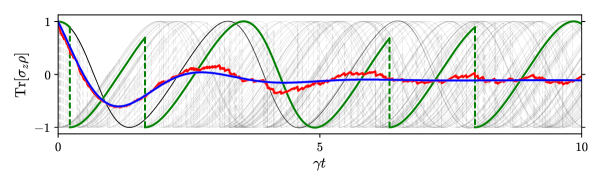
Figure 17: Comparison of photon-counting conditional evolution to unconditional open-system dynamics. The smooth blue curve in the foreground is the unconditional evolution. The jagged red curve that closely follows the unconditional evolution is the ensemble average of 64 photon-counting trajectories, which are also displayed as wispy grayscale traces in the background. A single trajectory from that ensemble is highlighted in green, exhibiting discontinuous evolution at times when photons were detected (represented by dashed vertical lines) connected by smooth, nonlinear modifications to ordinary Rabi oscillations arising from the backaction of the “no photon” measurement result.

If we instead monitor the waveguide with homodyne measurements, the system undergoes qualitatively different evolution. The system state never jumps, but vacuum fluctuations appear as jagged white-noise effects in the trajectory. One instance of a stochastic homodyne trajectory is highlighted in green in the upper-right-hand corner of Fig. 18. The other plots in Fig. 18 provide some intuition regarding what effects the squeezing and thermalization of the bath have on the system.

Figure 18: Comparison of homodyne trajectories and unconditional evolutions for squeezed, vacuum, antisqueezed, and thermal baths. The interpretation of the various curves is analogous to Fig. 17: the smooth blue curves in the foreground are the unconditional dynamics, the jagged red curves that approximate those dynamics are ensemble averages over the 64 trajectories plotted in the background in faint grayscale, and one member of that ensemble is highlighted in green. As one might expect, fluctuations in the homodyne trajectories decrease (increase) for the squeezed (antisqueezed, thermal) bath relative to the vacuum. Astute observers might notice that the conditional expectation values sometimes exceed the range of the observable’s spectrum. While it might be tempting to attribute this to some fundamental property of the interaction, these excesses are in fact artefacts of the finite integration step size and indicate an unphysical density matrix with negative eigenvalues. The unconditional evolutions exhibit less (more) damping for antisqueezed (squeezed, thermal) baths relative to the vacuum. This is due to a combination of how much information from the system is being lost to the environment (more for squeezed, less for antisqueezed) and how much noise from the environment is polluting the system (thermal noise in the case of the thermal bath).

The expression that various SMEs are “unravelings” of the unconditional master equation is meant to communicate that averages of larger and larger ensembles of trajectories converge to the unconditional evolution. These ensemble averages are presented in Figs. 17 and 18 as the jagged red curves closely hugging the smooth, blue curves of the unconditional evolution. For finite ensembles of trajectories, one still sees vestigial qualities of the underlying stochastic evolution, although the average trajectories are visibly converging to the unconditional evolution.

IX Discussion and Conclusion

We have now completed our introduction to trajectory theory, using only a minimal understanding of quantum optics to construct an interaction unitary and iterated quantum circuit. From that starting point, we built up the Gaussian theory using tools from finite-dimensional quantum information and computation. We found quantum circuits to illuminate the variety of conditions required to make the Markov approximations. We also found that all the relevant qualities of Gaussian bath modes can be compressed into the single transition of a qubit probe, capturing the effects of mean fields with infinitesimal rotations, thermal excitations with enhanced coupling, and squeezing with modified correlations between system operators $c$ and $c^{\dagger}$ in the interaction. We also explored an alternative means of producing weak interactions with an environment, noting that stretches of isolation punctuated by strong probe interactions can yield unconditional open-system dynamics similar to that of continuous weak interactions, but the conditional stochastic dynamics remain irreconcilably distinct.

Our program of qubit-izing continuous quantum measurements could be extended in several ways. For instance, one can imagine defining a wavepacket single-photon creation operator for $N$ qubits as

$$B^{\dagger}(\xi)=\sum_{n=1}^{N}\xi_{i}\sigma_{+}^{(n)}\quad\text{where}\quad\sum_{n}|\xi_{n}|^{2}=1\,.$$ (214)

Applying this to the multiqubit “vacuum” yields the single-photon state

$$\left|{1_{\xi}}\right\rangle=B^{\dagger}(\xi)\left|{ggg\ldots g}\right\rangle=\xi_{1}\left|{egg\ldots g}\right\rangle+\xi_{2}\left|{geg\ldots g}\right\rangle+\xi_{3}\left|{gge...g}\right\rangle+\cdots+\xi_{N}\left|{ggg\ldots e}\right\rangle.$$ (215)

Quantum trajectories for the single-photon Gough et al. (2011, 2012) and $N$-photon case Baragiola and Combes (2017) could be derived and studied, just as we did for the Gaussian cases. Da̧browska et al. have done recent work along these lines Da̧browska (2017); Da̧browska et al. (2017).

In addition to investigating different kinds of states, interactions, and measurements, we could also imagine trying to reproduce Carmichael’s Carmichael (1993b) and Gardiner’s Gardiner (1993) cascaded quantum systems formalism (and its generalization Gough and James (2009); Combes et al. (2017)). In the Markov approximation and the limit of zero delay between successive systems, we could imagine using an input-output formalism for probe qubits, of the sort alluded to at the end of Section VI.2, to connect successive systems, or we could work directly in the interaction picture as we have done throughout this paper.

Such extensions hold the promise of identifying parsimonious descriptions of the associated theory, but ultimately, we believe our approach can produce fruit beyond economy of description. The tools we emphasized encourage a particular way of thinking about continuous measurements, trajectories, and feedback that we believe is conducive to the development of improved forms of quantum control.

Acknowledgments: The authors thank Ben Baragiola and Rafael Alexander. JG, JC, and CMC were supported in part by National Science Foundation Grant Nos. PHY-1521016 and PHY-1314763 and by Office of Naval Research Grant No. N00014-11-1-0082. JC was supported in part by the Australian Research Council through a Discovery Early Career Researcher Award (DE160100356) and by the Perimeter Institute for Theoretical Physics. Research at the Perimeter Institute is supported by the Government of Canada through the Department of Innovation, Science and Economic Development Canada and by the Province of Ontario through the Ministry of Research, Innovation and Science. GJM and JC were supported via the Centre of Excellence in Engineered Quantum Systems (EQuS), Project Number CE110001013.

Appendix A Pure and thermal squeezed baths

In this Appendix we list relations that are useful for deriving the results for pure and thermal squeezed baths. The expressions involve the squeezed system operator $c_{\text{sq}}$ of Eq. 174 and the homodyne angle $\varphi_{\text{sq}}$ of Eq. 181. When written in terms of the squeezing parameters, $r$ and $\mu$, the expressions are indifferent to whether the bath is pure or thermal; when written in terms of the bath parameters, $N$, $M$, and $N_{\text{th}}$, the expressions use Eqs. (188b) and (188c), applicable for a squeezed thermal bath, to convert from the squeezing parameters to the bath parameters. To specialize the same expressions to a pure squeezed bath, one sets $N_{\text{th}}=0$.

Now the formulas:

$$\cosh^{2}\!r =\frac{N+N_{\text{th}}+1}{2N_{\text{th}}+1}\,,$$ (216)

$$\sinh^{2}\!r =\frac{N-N_{\text{th}}}{2N_{\text{th}}+1}\,,$$ (217)

$$e^{2i\mu}\sinh r\cosh r =-\frac{M}{2N_{\text{th}}+1}\,,$$ (218)

$$L =1+2\sinh^{2}\!r-2\cos 2\mu\,\sinh r\cosh r=\frac{2N+2M_{R}+1}{2N_{\text{th}}+1}=\frac{L^{\prime}}{2N_{\text{th}}+1}\,,$$ (219)

$$L^{\prime} =(2N_{\text{th}}+1)L=2N+2M_{R}+1\;,$$ (220)

$$\begin{split}e^{i\varphi_{\text{sq}}}c_{\text{sq}}&=\frac{c\,(\cosh^{2}\!r-e^{-2i\mu}\sinh r\cosh r)+c^{\dagger}(e^{2i\mu}\sinh r\cosh r-\sinh^{2}\!r)}{\sqrt{L}}\\ &=\frac{c\,(N+N_{\text{th}}+M^{*}+1)-c^{\dagger}(N-N_{\text{th}}+M)}{\sqrt{2N_{\text{th}}+1}\sqrt{L^{\prime}}}\,,\end{split}$$ (221)

$$\begin{split}c_{\text{sq}}\rho c^{\dagger}_{\text{sq}}&=c\rho c^{\dagger}\cosh^{2}\!r+c^{\dagger}\rho c\,\sinh^{2}\!r+c\rho c\,e^{-2i\mu}\sinh r\cosh r+c^{\dagger}\rho c^{\dagger}e^{2i\mu}\sinh r\cosh r\\ &=\frac{c\rho c^{\dagger}(N+N_{\text{th}}+1)+c^{\dagger}\rho c\,(N-N_{\text{th}})-c\rho c\,M^{*}-c^{\dagger}\rho c^{\dagger}M}{2N_{\text{th}}+1}\,,\end{split}$$ (222)

$$\begin{split}c^{\dagger}_{\text{sq}}c_{\text{sq}}&=c^{\dagger}c\,\cosh^{2}\!r+cc^{\dagger}\sinh^{2}\!r+c^{2}e^{-2i\mu}\sinh r\cosh r+{c^{\dagger}}^{2}e^{2i\mu}\sinh r\cosh r\\ &=\frac{c^{\dagger}c\,(N+N_{\text{th}}+1)+cc^{\dagger}(N-N_{\text{th}})-c^{2}\,M^{*}-{c^{\dagger}}^{2}M}{2N_{\text{th}}+1}\,,\end{split}$$ (223)

$$\mathcal{D}\left[{c_{\text{sq}}}\right]\rho =\frac{1}{2N_{\text{th}}+1}\!\left((N+N_{\text{th}}+1)\mathcal{D}[c]\rho+(N-N_{\text{th}})\mathcal{D}[c^{\dagger}]\rho+\frac{1}{2}M^{*}[c,[c,\rho]]+\frac{1}{2}M[c^{\dagger},[c^{\dagger},\rho]]\right)\,,$$ (224)

$$\begin{split}c^{\dagger}_{\text{sq}}\rho c_{\text{sq}}&=c^{\dagger}\rho c\,\cosh^{2}\!r+c\rho c^{\dagger}\sinh^{2}\!r+c\rho c\,e^{-2i\mu}\sinh r\cosh r+c^{\dagger}\rho c^{\dagger}e^{2i\mu}\sinh r\cosh r\\ &=\frac{c^{\dagger}\rho c\,(N+N_{\text{th}}+1)+c\rho c^{\dagger}(N-N_{\text{th}})-c\rho c\,M^{*}-c^{\dagger}\rho c^{\dagger}M}{2N_{\text{th}}+1}\,,\end{split}$$ (225)

$$\begin{split}c_{\text{sq}}c^{\dagger}_{\text{sq}}&=cc^{\dagger}\cosh^{2}\!r+c^{\dagger}c\,\sinh^{2}\!r+c^{2}\,e^{-2i\mu}\sinh r\cosh r+{c^{\dagger}}^{2}e^{2i\mu}\sinh r\cosh r\\ &=\frac{cc^{\dagger}(N+N_{\text{th}}+1)+c^{\dagger}c\,(N-N_{\text{th}})-c^{2}M^{*}-{c^{\dagger}}^{2}M}{2N_{\text{th}}+1}\,,\end{split}$$ (226)

$$\mathcal{D}\left[{c^{\dagger}_{\text{sq}}}\right]\rho =\frac{1}{2N_{\text{th}}+1}\!\left((N+N_{\text{th}}+1)\mathcal{D}[c^{\dagger}]\rho+(N-N_{\text{th}})\mathcal{D}[c]\rho+\frac{1}{2}M^{*}[c,[c,\rho]]+\frac{1}{2}M[c^{\dagger},[c^{\dagger},\rho]]\right)\,.$$ (227)

Appendix B Mixed squeezed states

To evaluate potential qubit models for mixed squeezed states, it is convenient to derive necessary and sufficient conditions on the combination of bath state $\sigma$, probe operator $a$, and measured observable for reproducing the stochastic evolution for homodyne detection, much as Eqs. (131) provide necessary and sufficient conditions on the bath state and probe operator for reproducing the unconditional evolution. Since the mixed nature of the bath generally introduces mixing into the system even when the bath is monitored, it is necessary to have at least four Kraus operators; this allows for two measurement outcomes and a conditional evolution for each of those outcomes, which is coarse-grained over two different Kraus evolutions corresponding to the other two outcomes. These Kraus operators can arise from a four-level probe in a pure initial state $\left|{\Phi}\right\rangle$ and observable eigenvectors $\left|{\pm\mathbin{\widetilde{\pm}}}\right\rangle$ (where the $\mathbin{\widetilde{\pm}}$ degree of freedom is coarse-grained over to reflect incomplete information) or from a pair of two-level probes in a mixed initial state $\lambda_{\mathbin{\widetilde{+}}}\left|{\psi_{\mathbin{\widetilde{+}}}}\middle\rangle\middle\langle{\psi_{\mathbin{\widetilde{+}}}}\right|+\lambda_{\mathbin{\widetilde{-}}}\left|{\psi_{\mathbin{\widetilde{-}}}}\middle\rangle\middle\langle{\psi_{\mathbin{\widetilde{-}}}}\right|$ and observable eigenvectors $\left|{\pm}\right\rangle$. When we use these arrangements with the interaction unitary

$$U_{I}(a) \mathrel{\mathop{:}}=\exp\left[\sqrt{\!\Delta\tau}\,\left(c\otimes a^{\dagger}-c^{\dagger}\otimes a\right)\right]\,,$$ (228)

where $a$ is a finite-dimensional operator analogous to the field annihilation operator $b$, we parametrize the resulting Kraus operators up to $\mathcal{O}(\Delta\tau)$ as

$$\begin{split}K_{\pm\mathbin{\widetilde{\pm}}}&=\left\langle{U_{I}}\right\rangle_{\pm\mathbin{\widetilde{\pm}}}\\ &=\alpha_{\pm\mathbin{\widetilde{\pm}}}+\sqrt{\!\Delta\tau}\,\!\left(\beta_{0\pm\mathbin{\widetilde{\pm}}}\,c+\beta_{1\pm\mathbin{\widetilde{\pm}}}\,c^{\dagger}\right)+\Delta\tau\!\left(\gamma_{0\pm\mathbin{\widetilde{\pm}}}\,c^{2}+\gamma_{1\pm\mathbin{\widetilde{\pm}}}\,cc^{\dagger}+\gamma_{2\pm\mathbin{\widetilde{\pm}}}\,c^{\dagger}c+\gamma_{3\pm\mathbin{\widetilde{\pm}}}\,{c^{\dagger}}^{2}\right)\,.\end{split}$$ (229)

Here we introduce the notation that for any operator $A$, $\left\langle{A}\right\rangle_{\pm\mathbin{\widetilde{\pm}}}\mathrel{\mathop{:}}=\left\langle{\pm\mathbin{\widetilde{\pm}}}\right|A\left|{\Phi}\right\rangle$ for the case of a pure bath with four measurement outcomes and $\left\langle{A}\right\rangle_{\pm\mathbin{\widetilde{\pm}}}\mathrel{\mathop{:}}=\sqrt{\lambda_{\mathbin{\widetilde{\pm}}}}\left\langle{\pm}\right|A\left|{\psi_{\mathbin{\widetilde{\pm}}}}\right\rangle$ for a mixed bath with two measurement outcomes. With this notation, the various parameters become

$$\alpha_{\pm\mathbin{\widetilde{\pm}}} =\vphantom{\frac{1}{2}}\left\langle{\mathds{1}}\right\rangle_{\pm\mathbin{\widetilde{\pm}}}\,,$$ (230a)

$$\beta_{0\pm\mathbin{\widetilde{\pm}}} =\vphantom{\frac{1}{2}}\big{\langle}a^{\dagger}\big{\rangle}_{\pm\mathbin{\widetilde{\pm}}}\,, \beta_{1\pm\mathbin{\widetilde{\pm}}} =-\big{\langle}a\big{\rangle}_{\pm\mathbin{\widetilde{\pm}}}\,,$$ (230b)

$$\gamma_{1\pm\mathbin{\widetilde{\pm}}} =-\frac{1}{2}\big{\langle}a^{\dagger}a\big{\rangle}_{\pm\mathbin{\widetilde{\pm}}}\,, \gamma_{2\pm\mathbin{\widetilde{\pm}}} =-\frac{1}{2}\big{\langle}aa^{\dagger}\big{\rangle}_{\pm\mathbin{\widetilde{\pm}}}\,,$$ (230c)

$$\gamma_{0\pm\mathbin{\widetilde{\pm}}} =\frac{1}{2}\big{\langle}{a^{\dagger}}^{2}\big{\rangle}_{\pm\mathbin{\widetilde{\pm}}}\,, \gamma_{3\pm\mathbin{\widetilde{\pm}}} =\frac{1}{2}\big{\langle}a^{2}\big{\rangle}_{\pm\mathbin{\widetilde{\pm}}}\,.$$ (230d)

Just like the case of a thermal bath, the updated state is calculated by coarse-graining over one of the two binary variables in the measurement outcome, giving

$$\rho_{\pm}=\frac{K_{\pm\mathbin{\widetilde{+}}}\rho K_{\pm\mathbin{\widetilde{+}}}^{\dagger}+K_{\pm\mathbin{\widetilde{-}}}\rho K_{\pm\mathbin{\widetilde{-}}}^{\dagger}}{\operatorname{Tr}[(E_{\pm}\rho]}\,,$$ (231)

where $E_{\pm}=K_{\pm\mathbin{\widetilde{+}}}^{\dagger}K_{\pm\mathbin{\widetilde{+}}}+K_{\pm\mathbin{\widetilde{-}}}^{\dagger}\rho K_{\pm\mathbin{\widetilde{-}}}$.

If we calculate the conditional difference equation from the parametrized Kraus operators (229), we can match terms to the squeezed-bath conditional difference equation (197) and come up with a set of constraints on the Kraus parameters. For the $\alpha$ parameters, we get

$$\alpha_{\pm\mathbin{\widetilde{+}}} =\frac{1}{\sqrt{2}}\cos\phi_{\pm}\,,$$ (232a)

$$\alpha_{\pm\mathbin{\widetilde{-}}} =\frac{1}{\sqrt{2}}\sin\phi_{\pm}\,,$$ (232b)

where we use the phase freedom inherent in the Kraus operators to make $\alpha_{\pm\mathbin{\widetilde{\pm}}}\geq 0$, i.e., $0\leq\phi_{\pm}\leq\pi/2$. The constraints for the $\beta$ parameters are

$$\left|\beta_{0\pm\mathbin{\widetilde{+}}}\right|^{2}+\left|\beta_{0\pm\mathbin{\widetilde{-}}}\right|^{2} =\frac{N+1}{2}\,,$$ (233a)

$$\left|\beta_{1\pm\mathbin{\widetilde{+}}}\right|^{2}+\left|\beta_{1\pm\mathbin{\widetilde{-}}}\right|^{2} =\frac{N}{2}\,,$$ (233b)

$$\beta_{1\pm\mathbin{\widetilde{+}}}\beta_{0\pm\mathbin{\widetilde{+}}}^{*}+\beta_{1\pm\mathbin{\widetilde{-}}}\beta_{0\pm\mathbin{\widetilde{-}}}^{*} =-\frac{M}{2}\,,$$ (233c)

$$\beta_{0\pm\mathbin{\widetilde{+}}}\cos\phi_{\pm}+\beta_{0\pm\mathbin{\widetilde{-}}}\sin\phi_{\pm} =\pm\frac{N+M^{*}+1}{\sqrt{2L^{\prime}}}\,,$$ (233d)

$$\beta_{1\pm\mathbin{\widetilde{+}}}\cos\phi_{\pm}+\beta_{1\pm\mathbin{\widetilde{-}}}\sin\phi_{\pm} =\mp\frac{N+M}{\sqrt{2L^{\prime}}}\,,$$ (233e)

where $L^{\prime}=2N+M+M^{*}+1$ as in Eq. 196. The nature of the constraints on the $\gamma$ variables always allows appropriate values to be found, given any solution of the above equations:

$$\gamma_{1\pm\mathbin{\widetilde{\pm}}} =-\frac{N}{4\sin(\phi_{\pm}+\pi/4)}\,,$$ (234a)

$$\gamma_{2\pm\mathbin{\widetilde{\pm}}} =-\frac{N+1}{4\sin(\phi_{\pm}+\pi/4)}\,,$$ (234b)

$$\gamma_{3\pm\mathbin{\widetilde{\pm}}} =-\frac{M}{4\sin(\phi_{\pm}+\pi/4)}\,,$$ (234c)

$$\gamma_{0\pm\mathbin{\widetilde{\pm}}} =-\frac{M^{*}}{4\sin(\phi_{\pm}+\pi/4)}\,.$$ (234d)

B.1 Araki-Woods

One technique that presents itself for the squeezed thermal case is the Araki-Woods construction, employed in Gough (2003) to treat general Gaussian states with a vacuum-based technique. This construction transforms the bath statistics from the probe state to the field operator in a slightly different manner than the successful technique and puts the probe into a two-mode vacuum. The form of the updated field operators is

$$b_{\text{AW}} \mathrel{\mathop{:}}=x(\mathds{1}\otimes b)+y(b^{\dagger}\otimes\mathds{1})+z(b\otimes\mathds{1})\,,$$ (235)

corresponding to a qubit model with probe initial state $\left|{gg}\right\rangle$ and updated qubit field operators

$$a_{\text{AW}}\mathrel{\mathop{:}}=x(\mathds{1}\otimes\sigma_{-})+y(\sigma_{+}\otimes\mathds{1})+z(\sigma_{-}\otimes\mathds{1})\,,$$ (236)

where the constants $x$, $y$, and $z$ are defined as

$$x \mathrel{\mathop{:}}=\sqrt{N+1-\left|M\right|^{2}/N}\,,$$ (237a)

$$y \mathrel{\mathop{:}}=\sqrt{N}\,,$$ (237b)

$$z \mathrel{\mathop{:}}=M/\sqrt{N}\,.$$ (237c)

The above definitions are slightly different from those presented in Gough (2003), as we have suppressed the mean field term, it being trivial to include such a term, as is described at the end of Section VI.5, and changed the ordering of the subsystems to reflect our notational conventions.

When the bath is in a pure state, $\left|M\right|^{2}=N(N+1)$ and thus $x=0$. Since the only term in $a_{\text{AW}}$ that involves the second is proportional to $x$, for a pure bath we only need to consider the first field mode. In this case, using $a_{\text{AW}}$ in the interaction unitary and measuring $a_{\text{AW}}+a_{\text{AW}}^{\dagger}$ gives the Kraus operators Eq. 182 and therefore produces the correct stochastic evolution.

Unfortunately, even though the Araki-Woods discrete field operators give the appropriate bath statistics and thus the correct unconditional evolution even for $\left|M\right|^{2}<N(N+1)$, they do not satisfy the constraints given above to produce the correct conditional evolution. In particular, the Araki-Woods Kraus operators give us

$$\cos\phi_{\pm} =\sin\phi_{\pm}=\frac{1}{\sqrt{2}}\,,$$ (238a)

$$\beta_{0\pm\mathbin{\widetilde{+}}}+\beta_{0\pm\mathbin{\widetilde{-}}} =\pm\frac{N+M^{*}+1}{\sqrt{L^{\prime}}}\sqrt{\frac{N+2M_{R}+\left|M\right|^{2}/N}{2N+2M_{R}+1}}\,.$$ (238b)

This only satisfies the SME constraints when $|M|^{2}=N(N+1)$, i.e., when the bath is in a pure state.

One indication that something might break in the mixed case is that the field homodyne observable, $b_{\text{AW}}+b_{\text{AW}}^{\dagger}$, ought to have degeneracy in eigenvalues, since in the field picture the thermalization of the field can be interpreted as entanglement with an auxiliary mode that is not measured (i.e., we measure $(b+b^{\dagger})\otimes\mathds{1}$), leading to degenerate subspaces for each eigenvalue of $b+b^{\dagger}$. In the qubit picture, the homodyne observable $a_{\text{AW}}+a_{\text{AW}}^{\dagger}$ has the spectrum

$$\lambda_{\pm\mathbin{\widetilde{\pm}}} =\mathbin{\widetilde{\pm}}x\pm\left|y+z\right|\,,$$ (239)

which is degenerate only in the case $x=0$, since $\left|z\right|\leq\sqrt{y^{2}+1}\leq y$ from Eq. 124. This condition is met only when the bath is pure.

B.2 Two-qubit setup analogous to two-mode squeezing

To manufacture thermal statistics, we might think to consider the thermal state of a bath mode as the marginal state of a two-mode squeezed state. Then, much as we did in the pure-state case, we could transfer all squeezing from the bath state to the field operators and on to analogous qubit operators. Using the two-mode squeeze operator,

$$S^{(1,2)}(r_{\text{th}}) \mathrel{\mathop{:}}=\exp\left[r_{\text{th}}\left(b\otimes b-b^{\dagger}\!\otimes b^{\dagger}\right)\right]\,,$$ (240)

gives us the squeezed field operator

$$b_{\text{sq}} ={S^{(12)}}^{\dagger}\!(r_{\text{th}})\,{S^{(1)}}^{\dagger}\!(r,\phi)\,(b\otimes\mathds{1})\,S^{(1)}(r,\phi)\,S^{(12)}(r_{\text{th}})$$ (241)

$$=\cosh r\cosh r_{\text{th}}(b\otimes\mathds{1})-e^{2i\phi}\cosh r\sinh r_{\text{th}}(\mathds{1}\otimes b^{\dagger})-e^{2i\phi}\sinh r\cosh r_{\text{th}}(b^{\dagger}\otimes\mathds{1})+\sinh r\sinh r_{\text{th}}(\mathds{1}\otimes b)\,,$$ (242)

which translates to the squeezed qubit operators

$$a_{\text{sq}} =\cosh r\cosh r_{\text{th}}(\sigma_{-}\otimes\mathds{1})-e^{2i\phi}\cosh r\sinh r_{\text{th}}(\mathds{1}\otimes\sigma_{+})-e^{2i\phi}\sinh r\cosh r_{\text{th}}(\sigma_{+}\otimes\mathds{1})+\sinh r\sinh r_{\text{th}}(\mathds{1}\otimes\sigma_{-})\,.$$ (243)

The quadrature operator for homodyne measurement, $a_{\text{sq}}+a_{\text{sq}}^{\dagger}$, has a problem similar to that of the Araki-Woods quadrature operator in that its eigenvalues are nondegenerate:

$$\lambda_{1\pm} =\pm\frac{1}{\sqrt{2}e^{r}}\sqrt{-e^{4r}e^{2r_{\text{th}}}\cos 2\phi+e^{4r}e^{2r_{\text{th}}}+e^{2r_{\text{th}}}\cos 2\phi+e^{2r_{\text{th}}}}\,,$$ (244)

$$\lambda_{2\pm} =\pm\frac{1}{\sqrt{2}e^{r}e^{r_{\text{th}}}}\sqrt{-e^{4r}\cos 2\phi+e^{4r}+1+\cos 2\phi}\,.$$ (245)

This construction fails to satisfy the Kraus-operator constraints on thermal stochastic evolution even in the absence of squeezing ($N>0$, $M=0$), confirming our suspicion based on the nondegeneracy of the observable eigenvalues.

B.3 Two-qubit squeezed-thermal state

Another simple two-qubit setup uses the probe annihilation operator

$$a_{\text{sq}} =\sqrt{\frac{2N+1}{2}}(\mathds{1}\otimes\sigma_{-}+\sigma_{-}\otimes\mathds{1})$$ (246)

in conjunction with the interaction unitary $U(a_{\text{sq}})$ from Eq. 228 and the initial probe state

$$\sigma_{\text{sq}} =\frac{1}{2N+1}\begin{pmatrix}N&0&0&M\\ 0&0&0&0\\ 0&0&0&0\\ M^{*}&0&0&N+1\end{pmatrix}\,,$$ (247)

which we consider as it is a positive state precisely when the parameters $M$ and $N$ satisfy the usual constraint $|M|^{2}\leq(N+1)N$ (obtaining purity only when $|M|^{2}=(N+1)N$). By observation or by calculation, we see that the bath density operator has rank two, i.e., has support only on a qubit subspace.

The consequences of this model are analogous to those of the Araki-Woods construction: unconditional statistics are reproduced, but the stochastic evolution is incorrect when measuring $a_{\text{sq}}+a_{\text{sq}}^{\dagger}$. The difficulty again appears to be a lack of degeneracy in the eigenvalues of the $a_{\text{sq}}+a_{\text{sq}}^{\dagger}$. Specifically, this setup reproduces the correct bath statistics, but the observable $a_{\text{sq}}+a_{\text{sq}}^{\dagger}$ has three distinct eigenvalues (unique positive and negative eigenvalues with a twofold degeneracy corresponding to an eigenvalue of 0) instead of degenerate positive and negative subspaces as we expect from the field case.

Naïvely pairing half of the zero subspace with both the positive and negative outcomes yields a SME in the pure case very close to the correct result, except that the Wiener process $dW$ is divided by $\sqrt{2(2N+1)}$ instead of $\sqrt{L^{\prime}}$; this corresponds to doing homodyne detection on a pure squeezed bath with detectors having subunity efficiency. Likewise, setting $M=0$ for a thermal bath with no squeezing yields a thermal SME with an extra factor of $1/\sqrt{2}$ in the stochastic term, again analogous to subunity detection efficiency.

This inefficiency makes sense given that we naïvely lumped distinguishable measurement outcomes together. Unfortunately, this model doesn’t provide clear alternative recipes with which to construct a SME, so we don’t consider this model any further.

B.4 Qutrit

One can also mock up a bath with three-level probes and field operators that give the correct unconditional evolution. We define the qutrit probe annihilation operator to be

$$a:=\sqrt{2N+1}\big{(}\left|{0}\right\rangle\left\langle{1}\right|+\left|{1}\right\rangle\left\langle{2}\right|\big{)}\,.$$ (248)

The thermal and squeezed qutrit probe state we choose, following the reasoning by which we arrived at Eq. 247, is

$$\sigma_{\text{sq}}:=\frac{1}{2N+1}\begin{pmatrix}N&0&M\\ 0&0&0\\ M^{*}&0&N+1\end{pmatrix}\,.$$ (249)

In our matrix representations we have ordered the rows and columns starting from the top and left with $\left|{2}\right\rangle$ and decreasing to $\left|{0}\right\rangle$ as we move to the bottom and right.

The combination of the above lowering operator and state gives the correct unconditional master equation. Three-level systems present even more difficulty in understanding what to do with the conditional evolution, however, as the restriction to three Kraus operators means only one of the measurement results can be coarse-grained over multiple (two) Kraus operators, leaving the other measurement result only associated with a single Kraus operator and therefore producing no statistical mixing of the system state.

References

• Hood et al. (1998) C. J. Hood, M. S. Chapman, T. W. Lynn,  and H. J. Kimble, “Real-time cavity QED with single atoms,” Phys. Rev. Lett. 80, 4157 (1998).
• Gambetta et al. (2008) J. Gambetta, A. Blais, M. Boissonneault, A. A. Houck, D. I. Schuster,  and S. M. Girvin, “Quantum trajectory approach to circuit QED: Quantum jumps and the Zeno effect,” Phys. Rev. A 77, 012112 (2008).
• Boissonneault et al. (2008) M. Boissonneault, J. M. Gambetta,  and A. Blais, “Nonlinear dispersive regime of cavity QED: The dressed dephasing model,” Phys. Rev. A 77, 060305 (2008).
• Murch et al. (2013) K. W. Murch, S. J. Weber, C. Macklin,  and I. Siddiqi, “Observing single quantum trajectories of a superconducting quantum bit,” Nature 502, 211 (2013).
• Goan and Milburn (2001) H.-S. Goan and G. J. Milburn, “Dynamics of a mesoscopic charge quantum bit under continuous quantum measurement,” Phys. Rev. B 64, 235307 (2001).
• Oxtoby et al. (2005) N. P. Oxtoby, P. Warszawski, H. M. Wiseman, H.-B. Sun,  and R. E. S. Polkinghorne, “Quantum trajectories for the realistic measurement of a solid-state charge qubit,” Phys. Rev. B 71, 165317 (2005).
• Oxtoby et al. (2008) N. P. Oxtoby, J. Gambetta,  and H. M. Wiseman, “Model for monitoring of a charge qubit using a radio-frequency quantum point contact including experimental imperfections,” Phys. Rev. B 77, 125304 (2008).
• Milburn et al. (1994) G. J. Milburn, K. Jacobs,  and D. F. Walls, “Quantum-limited measurements with the atomic force microscope,” Phys. Rev. A 50, 5256 (1994).
• Hopkins et al. (2003) A. Hopkins, K. Jacobs, S. Habib,  and K. Schwab, “Feedback cooling of a nanomechanical resonator,” Phys. Rev. B 68, 235328 (2003).
• Ruskov et al. (2005) R. Ruskov, K. Schwab,  and A. N. Korotkov, “Squeezing of a nanomechanical resonator by quantum nondemolition measurement and feedback,” Phys. Rev. B 71, 235407 (2005).
• Jacobs et al. (2007) K. Jacobs, P. Lougovski,  and M. Blencowe, “Continuous measurement of the energy eigenstates of a nanomechanical resonator without a nondemolition probe,” Phys. Rev. Lett. 98, 147201 (2007).
• Ahn et al. (2002) C. Ahn, A. C. Doherty,  and A. J. Landahl, “Continuous quantum error correction via quantum feedback control,” Phys. Rev. A 65, 042301 (2002).
• Sarovar et al. (2004) M. Sarovar, C. Ahn, K. Jacobs,  and G. J. Milburn, “Practical scheme for error control using feedback,” Phys. Rev. A 69, 052324 (2004).
• Ahn et al. (2004) C. Ahn, H. Wiseman,  and K. Jacobs, “Quantum error correction for continuously detected errors with any number of error channels per qubit,” Phys. Rev. A 70, 024302 (2004).
• Gregoratti and Werner (2004) M. Gregoratti and R. F. Werner, “On quantum error-correction by classical feedback in discrete time,” Journal of Mathematical Physics 45, 2600 (2004).
• van Handel and Mabuchi (2005) R. van Handel and H. Mabuchi, “Optimal error tracking via quantum coding and continuous syndrome measurement,” quant-ph/0511221  (2005).
• Chase et al. (2008) B. A. Chase, A. J. Landahl,  and J. Geremia, “Efficient feedback controllers for continuous-time quantum error correction,” Phys. Rev. A 77, 032304 (2008).
• Mabuchi (2009) H. Mabuchi, “Continuous quantum error correction as classical hybrid control,” New Journal of Physics 11, 105044 (2009).
• Lidar and Brun (2013) D. A. Lidar and T. A. Brun, eds., Quantum Error Correction (Cambridge University Press, 2013).
• Nguyen et al. (2015) T. Nguyen, C. D. Hill, L. C. L. Hollenberg,  and M. R. James, “Surface code continuous quantum error correction using feedback,” in 2015 54th IEEE Conference on Decision and Control (CDC) (2015) pp. 7101–7106.
• Hsu and Brun (2016) K.-C. Hsu and T. A. Brun, “Method for quantum-jump continuous-time quantum error correction,” Phys. Rev. A 93, 022321 (2016).
• Oreshkov and Brun (2005) O. Oreshkov and T. A. Brun, “Weak measurements are universal,” Phys. Rev. Lett. 95, 110409 (2005).
• Varbanov and Brun (2007) M. Varbanov and T. A. Brun, “Decomposing generalized measurements into continuous stochastic processes,” Phys. Rev. A 76, 032104 (2007).
• Florjanczyk and Brun (2015) J. Florjanczyk and T. A. Brun, “Continuous decomposition of quantum measurements via Hamiltonian feedback,” Phys. Rev. A 92, 062113 (2015).
• Florjanczyk and Brun (2014) J. Florjanczyk and T. A. Brun, “Continuous decomposition of quantum measurements via qubit-probe feedback,” Phys. Rev. A 90, 032102 (2014).
• Mabuchi (1996) H. Mabuchi, “Dynamical identification of open quantum systems,” Quantum and Semiclassical Optics 8, 1103 (1996).
• Gambetta and Wiseman (2001) J. Gambetta and H. M. Wiseman, “State and dynamical parameter estimation for open quantum systems,” Phys. Rev. A 64, 042105 (2001).
• Chase and Geremia (2009) B. A. Chase and J. M. Geremia, “Single-shot parameter estimation via continuous quantum measurement,” Phys. Rev. A 79, 022314 (2009).
• Gammelmark and Mølmer (2013) S. Gammelmark and K. Mølmer, “Bayesian parameter inference from continuously monitored quantum systems,” Phys. Rev. A 87, 032115 (2013).
• Kiilerich and Mølmer (2014) A. H. Kiilerich and K. Mølmer, “Estimation of atomic interaction parameters by photon counting,” Phys. Rev. A 89, 052110 (2014).
• Kiilerich and Mølmer (2016) A. H. Kiilerich and K. Mølmer, “Bayesian parameter estimation by continuous homodyne detection,” Phys. Rev. A 94, 032103 (2016).
• Gong and Cui (2017) B. Gong and W. Cui, “On the calculation of Fisher information for quantum parameter estimation based on the stochastic master equation,” arXiv:1702.08089 [quant-ph]  (2017).
• Cook et al. (2014) R. L. Cook, C. A. Riofrío,  and I. H. Deutsch, “Single-shot quantum state estimation via a continuous measurement in the strong backaction regime,” Phys. Rev. A 90, 032113 (2014).
• Brun (2002) T. A. Brun, “A simple model of quantum trajectories,” American Journal of Physics 70, 719 (2002).
• Scully and Lamb (1967) M. O. Scully and W. E. Lamb, “Quantum theory of an optical maser. I. General theory,” Phys. Rev. 159, 208 (1967).
• Meyer (1986) P. Meyer, “A finite approximation to boson Fock space,” in Stochastic Processes in Classical and Quantum Systems (Springer, 1986) pp. 405–410.
• Attal (2002) S. Attal, “Approximating the Fock space with the toy Fock space,” Séminaire de Probabilités de Strasbourg 36, 477 (2002).
• Gough and Sobolev (2004) J. Gough and A. Sobolev, “Stochastic Schrödinger equations as limit of discrete filtering,” Open Systems & Information Dynamics 11, 235 (2004).
• Gough (2004) J. Gough, “Holevo-ordering and the continuous-time limit for open Floquet dynamics,” Letters in Mathematical Physics 67, 207 (2004).
• Attal and Pautrat (2005) S. Attal and Y. Pautrat, “From $(n+1)$-level atom chains to $n$-dimensional noises,” in Annales de l’Institut Henri Poincare (B) Probability and Statistics, Vol. 41 (Elsevier, 2005) pp. 391–407.
• Attal and Pautrat (2006) S. Attal and Y. Pautrat, “From repeated to continuous quantum interactions,” Annales Henri Poincaré 7, 59 (2006).
• Belton (2008) A. C. R. Belton, “Approximation via toy Fock space - the vacuum-adapted viewpoint,” in Quantum Stochastics and Information (World Scientific, 2008) pp. 3–22.
• Bouten et al. (2009) L. Bouten, R. van Handel,  and M. R. James, “A discrete invitation to quantum filtering and feedback control,” SIAM Review 51, 239 (2009).
• Attal and Nechita (2011) S. Attal and I. Nechita, “Discrete approximation of the free Fock space,” in Séminaire de Probabilités XLIII, edited by C. Donati-Martin, A. Lejay,  and A. Rouault (Springer Berlin Heidelberg, Berlin, Heidelberg, 2011) pp. 379–394.
• Mensky (1979) M. B. Mensky, “Quantum restrictions for continuous observation of an oscillator,” Phys. Rev. D 20, 384 (1979).
• Mensky (1993) M. B. Mensky, Continuous Quantum Measurements and Path Integrals (CRC Press, 1993).
• Belavkin (1980) V. P. Belavkin, “Quantum filtering of Markov signals with white quantum noise,” Radiotechnika i Electronika 25, 1445 (1980).
• Srinivas and Davies (1981) M. Srinivas and E. Davies, “Photon counting probabilities in quantum optics,” Optica Acta: International Journal of Optics 28, 981 (1981).
• Braginskiĭ and Khalili (1995) V. B. Braginskiĭ and F. Y. Khalili, Quantum Measurement (Cambridge University Press, 1995).
• Barchielli et al. (1982) A. Barchielli, L. Lanz,  and G. M. Prosperi, “A model for the macroscopic description and continual observations in quantum mechanics,” Il Nuovo Cimento B (1971-1996) 72, 79 (1982).
• Gisin (1984) N. Gisin, “Quantum measurements and stochastic processes,” Phys. Rev. Lett. 52, 1657 (1984).
• Diósi (1986) L. Diósi, “Stochastic pure state representation for open quantum systems,” Physics Letters A 114, 451 (1986).
• Diósi (1988) L. Diósi, “Continuous quantum measurement and Itô formalism,” Physics Letters A 129, 419 (1988).
• Caves (1986) C. M. Caves, “Quantum mechanics of measurements distributed in time. A path-integral formulation,” Phys. Rev. D 33, 1643 (1986).
• Caves (1987) C. M. Caves, “Quantum mechanics of measurements distributed in time. II. Connections among formulations,” Phys. Rev. D 35, 1815 (1987).
• Caves and Milburn (1987) C. M. Caves and G. J. Milburn, “Quantum-mechanical model for continuous position measurements,” Phys. Rev. A 36, 5543 (1987).
• Wiseman and Milburn (1993a) H. M. Wiseman and G. J. Milburn, “Quantum theory of field-quadrature measurements,” Phys. Rev. A 47, 642 (1993a).
• Carmichael (1993a) H. J. Carmichael, An Open Systems Approach to Quantum Optics, Lecture Notes in Physics Monographs, Vol. 18 (Springer-Verlag Berlin Heidelberg, 1993).
• Dalibard et al. (1992) J. Dalibard, Y. Castin,  and K. Mølmer, “Wave-function approach to dissipative processes in quantum optics,” Phys. Rev. Lett. 68, 580 (1992).
• Korotkov (1999) A. N. Korotkov, “Continuous quantum measurement of a double dot,” Phys. Rev. B 60, 5737 (1999).
• Korotkov (2001) A. N. Korotkov, “Selective quantum evolution of a qubit state due to continuous measurement,” Phys. Rev. B 63, 115403 (2001).
• Jacobs and Steck (2006) K. Jacobs and D. A. Steck, “A straightforward introduction to continuous quantum measurement,” Contemporary Physics 47, 279 (2006).
• Wiseman (1994a) H. M. Wiseman, Quantum trajectories and feedbackPh.D. thesis, University of Queensland (1994a).
• Bouten et al. (2007) L. Bouten, R. V. Handel,  and M. R. James, “An introduction to quantum filtering,” SIAM Journal on Control and Optimization 46, 2199 (2007).
• Carmichael (2008) H. J. Carmichael, Statistical Methods in Quantum Optics 2: Non-Classical Fields, Theoretical and Mathematical Physics (Springer-Verlag Berlin Heidelberg, 2008).
• Wiseman and Milburn (2010) H. M. Wiseman and G. J. Milburn, Quantum Measurement and Control (Cambridge University Press, 2010).
• Jacobs (2014) K. Jacobs, Quantum Measurement Theory and Its Applications (Cambridge University Press, 2014).
• Aharonov et al. (1988) Y. Aharonov, D. Z. Albert,  and L. Vaidman, “How the result of a measurement of a component of the spin of a spin-1/2 particle can turn out to be 100,” Phys. Rev. Lett. 60, 1351 (1988).
• Duck et al. (1989) I. M. Duck, P. M. Stevenson,  and E. C. G. Sudarshan, “The sense in which a ‘weak measurement’ of a spin-½ particle’s spin component yields a value 100,” Phys. Rev. D 40, 2112 (1989).
• Zoller et al. (1987) P. Zoller, M. Marte,  and D. F. Walls, “Quantum jumps in atomic systems,” Physical Review A 35, 198 (1987).
• Nielsen and Chuang (2010) M. A. Nielsen and I. L. Chuang, Quantum Computation and Quantum Information (Cambridge University Press, 2010).
• Doherty and Jacobs (1999) A. C. Doherty and K. Jacobs, “Feedback control of quantum systems using continuous state estimation,” Physical Review A 60, 2700 (1999).
• Gardiner and Zoller (2004) C. W. Gardiner and P. Zoller, Quantum Noise (Springer, 2004).
• Unruh and Zurek (1989) W. G. Unruh and W. H. Zurek, “Reduction of a wave packet in quantum Brownian motion,” Phys. Rev. D 40, 1071 (1989).
• Fischer et al. (2017) K. A. Fischer, R. Trivedi, V. Ramasesh, I. Siddiqi,  and J. Vučković, “Scattering of coherent pulses from quantum-optical systems,” arXiv:1710.02875  (2017).
• Sayrin et al. (2011) C. Sayrin, I. Dotsenko, X. Zhou, B. Peaudecerf, T. Rybarczyk, S. Gleyzes, P. Rouchon, M. Mirrahimi, H. Amini, M. Brune, J.-M. Raimond,  and S. Haroche, “Real-time quantum feedback prepares and stabilizes photon number states,” Nature 477, 73 (2011).
• Scully and Zubairy (1997) M. O. Scully and M. S. Zubairy, Quantum Optics (Cambridge University Press, 1997).
• Horowitz (2012) J. M. Horowitz, “Quantum-trajectory approach to the stochastic thermodynamics of a forced harmonic oscillator,” Phys. Rev. E 85, 031110 (2012).
• Strasberg et al. (2017) P. Strasberg, G. Schaller, T. Brandes,  and M. Esposito, “Quantum and information thermodynamics: A unifying framework based on repeated interactions,” Phys. Rev. X 7, 021003 (2017).
• Giovannetti and Palma (2012) V. Giovannetti and G. M. Palma, “Master equations for correlated quantum channels,” Phys. Rev. Lett. 108, 040401 (2012).
• Rybár et al. (2012) T. Rybár, S. N. Filippov, M. Ziman,  and V. Bužek, “Simulation of indivisible qubit channels in collision models,” Journal of Physics B: Atomic, Molecular and Optical Physics 45, 154006 (2012).
• Ciccarello (2017) F. Ciccarello, “Collision models in quantum optics,” arXiv:1712.04994 (To appear in Quantum Measurements and Quantum Metrology)  (2017).
• Gisin and Percival (1992) N. Gisin and I. C. Percival, “Wave-function approach to dissipative processes: Are there quantum jumps?” Physics Letters A 167, 315 (1992).
• Wiseman and Milburn (1993b) H. M. Wiseman and G. J. Milburn, “Interpretation of quantum jump and diffusion processes illustrated on the Bloch sphere,” Phys. Rev. A 47, 1652 (1993b).
• Wiseman (1994b) H. M. Wiseman, “Quantum theory of continuous feedback,” Phys. Rev. A 49, 2133 (1994b).
• Gardiner et al. (1992) C. W. Gardiner, A. S. Parkins,  and P. Zoller, “Wave-function quantum stochastic differential equations and quantum-jump simulation methods,” Phys. Rev. A 46, 4363 (1992).
• Dum et al. (1992) R. Dum, A. S. Parkins, P. Zoller,  and C. W. Gardiner, “Monte Carlo simulation of master equations in quantum optics for vacuum, thermal, and squeezed reservoirs,” Phys. Rev. A 46, 4382 (1992).
• Gough (2003) J. Gough, “Quantum white noises and the master equation for Gaussian reference states,” Russian Journal of Mathematical Physics 10, 142 (2003).
• Nechita and Pellegrini (2009) I. Nechita and C. Pellegrini, “Quantum trajectories in random environment: The statistical model for a heat bath,” Confluentes Mathematici 01, 249 (2009).
• Attal and Pellegrini (2010) S. Attal and C. Pellegrini, “Stochastic master equations in thermal environment,” Open Systems & Information Dynamics 17, 389 (2010).
• Hellmich et al. (2002) J. Hellmich, R. Honegger, C. Köstler, B. Kümmerer,  and A. Rieckers, “Couplings to classical and non-classical squeezed white noise as stationary Markov processes,” Publications of the Research Institute for Mathematical Sciences 38, 1 (2002).
• Haus and Mullen (1962) H. A. Haus and J. A. Mullen, “Quantum noise in linear amplifiers,” Phys. Rev. 128, 2407 (1962).
• Caves (1982) C. M. Caves, “Quantum limits on noise in linear amplifiers,” Phys. Rev. D 26, 1817 (1982).
• Yurke and Denker (1984) B. Yurke and J. S. Denker, “Quantum network theory,” Phys. Rev. A 29, 1419 (1984).
• Blow et al. (1990) K. J. Blow, R. Loudon, S. J. D. Phoenix,  and T. J. Shepherd, “Continuum fields in quantum optics,” Phys. Rev. A 42, 4102 (1990).
• Chiao and Garrison (2008) R. Y. Chiao and J. C. Garrison, Quantum Optics (Oxford University Press, 2008).
• Milburn (2014) G. J. Milburn, “Quantum control based on measurement,” in Quantum Information and Coherence, edited by E. Andersson and P. Öhberg (Springer, Berlin, 2014) pp. 147–158.
• Gross (2017) J. Gross, “Pysme: A package for simulating stochastic master equations in python,” github.com  (2017), DOI: 10.5281/zenodo.1034811.
• Kloeden and Platen (1992) P. E. Kloeden and E. Platen, Numerical Solution of Stochastic Differential Equations (Springer Berlin Heidelberg, Berlin, Heidelberg, 1992).
• Gough et al. (2011) J. E. Gough, M. R. James,  and H. I. Nurdin, “Quantum master equation and filter for systems driven by fields in a single photon state,” in Proceedings of the joint 50th IEEE Conference on Decision and Control and European Control Conference (CDC-ECC) (2011) pp. 5570–5576.
• Gough et al. (2012) J. E. Gough, M. R. James, H. I. Nurdin,  and J. Combes, “Quantum filtering for systems driven by fields in single-photon states or superposition of coherent states,” Phys. Rev. A 86, 043819 (2012).
• Baragiola and Combes (2017) B. Q. Baragiola and J. Combes, “Quantum trajectories for propagating Fock states,” Phys. Rev. A 96, 023819 (2017).
• Da̧browska (2017) A. Da̧browska, “Quantum trajectories for environment in superposition of coherent states,” arXiv:1707.06205  (2017).
• Da̧browska et al. (2017) A. Da̧browska, G. Sarbicki,  and D. Chruściński, “Quantum trajectories for a system interacting with environment in a single-photon state: Counting and diffusive processes,” Phys. Rev. A 96, 053819 (2017).
• Carmichael (1993b) H. J. Carmichael, “Quantum trajectory theory for cascaded open systems,” Phys. Rev. Lett. 70, 2273 (1993b).
• Gardiner (1993) C. W. Gardiner, “Driving a quantum system with the output field from another driven quantum system,” Phys. Rev. Lett. 70, 2269 (1993).
• Gough and James (2009) J. Gough and M. R. James, “The series product and its application to quantum feedforward and feedback networks,” IEEE Trans. Aut. Control 54, 2530 (2009).
• Combes et al. (2017) J. Combes, J. Kerckhoff,  and M. Sarovar, “The SLH framework for modeling quantum input-output networks,” Advances in Physics: X 2, 784 (2017).