Laplacian Prior Variational Automatic Relevance Determination for Transmission Tomography
Abstract
In the classic sparsity-driven problems, the fundamental L-1 penalty method has been shown to have good performance in reconstructing signals for a wide range of problems. However this performance relies on a good choice of penalty weight which is often found from empirical experiments. We propose an algorithm called the Laplacian variational automatic relevance determination (Lap-VARD) that takes this penalty weight as a parameter of a prior Laplace distribution. Optimization of this parameter using an automatic relevance determination framework results in a balance between the sparsity and accuracy of signal reconstruction. Our algorithm is implemented in a transmission tomography model with sparsity constraint in wavelet domain.
Index Terms:
Laplace distribution, automatic relevance determination(ARD), sparsity, LASSO, Transmission Tomography, wavelet, Poisson noise.I Introduction
Transmission tomography is a well-established and efficient method to represent the linear attenuation coefficient inside the image of interest. Among all the modalities, X-ray computed tomography (CT) [1] introduced into clinical use in 1972 is the earliest and also the most widely used one. The pursuit to get high resolution requires a large amount of measurement data; however, limitations of data storage and computation resources force a threshold on the resolution. To overcome these limitations, extra information of the image itself should be taken into consideration. The sparsity of image can be represented not only in the image domain, but also in a transformed domain like the directional gradient domain or wavelet transform domain [2][3].
In sparsity-driven problems, the basic idea is that when we know in advance that the image of interest is sparse or sparse in some basis, then we need fewer observations than the traditional methods to reconstruct the image using the significant components in the image [4]. For these problems, a universal method to seek a best sparse approximation is an L-1 penalty
where is the cost function, and is the data fitting term. This is equivalent to the L-1 regularization problem [5]
The problem to minimize (1.1) is called LASSO [6]. The optimal solution shrinks to 0 as the parameter goes to infinity, which means that the sparsity in the reconstruction is determined by the choice of . A very small yields low sparsity. However, if is too large, it over-penalizes and we have an all-zero image in the limit [7]. To get a balance between sparsity and data fitting, we propose the Lap-VARD algorithm to automatically update iteratively. Because in this algorithm depends on the measurements, it is an adaptive method.
This Lap-VARD is inspired by the fact that if we take in (1.1), and let the prior of be a zero-mean Laplace distribution: ,with and , then
Now, this problem becomes a MAP problem [8]. Instead of maximizing over , we take as hyper-parameter and try to maximize the marginal likelihood
This method is called automatic relevance determination (ARD) [9]. In [10], the AM-ARD method is taken into the Transmission Tomography model with a Gaussian Prior. In the Lap-VARD algorithm, we use the Laplace Prior to promote the sparsity and automatically get the best-fitting hyper-parameter in (1.1) to have a balance between sparsity and data-fitting.
II Proposed Method
In X-ray CT image reconstruction, the data fitting term is the negative log-likelihood of a Poisson distribution [11]
where is the image we try to reconstruct, is the X-ray photon measurement for source-detector pair , and is the mean of a Poisson random variable , is the air scan photon counts for source-detector pair , and is an element in the system matrix that represents the contribution of pixel to source-detector pair [12].
In [13], a wavelet sparsity penalty is introduced and the advantage of a wavelet sparsity penalty is that it does not generate biased reconstructions. The wavelet sparsity penalty is in the following form
where is the negative log-likelihood of a Laplace distribution with mean and variance . is the set of wavelet coefficients of image with the transform pair
and
where and . From (1.1), the overall cost function is
where
Reformulating the cost function in the wavelet coefficient domain only, the reformulated cost function is
| (2.6) |
where
Now, we have a new system matrix The performance of the reconstruction algorithm is controlled by the hyper-parameters . We use the ARD framework to find the optimal .
The marginal log-likelihood is
Then . Here, we rewrite the marginal log-likelihood as
| (2.9) |
where stands for the expected value with respect to , and is the Kullback-Leibler (KL) divergence.
From [14], we take a variational method to solve iteratively. Since the change of does not change the value of , then at iteration we set such that . we just need to maximize the first term in with respect to , which is called free variational energy (FVE). The EM algorithm [14] can be viewed as minimizing the FVE function by alternating between updating and . However, the expression for is complicated. As in VARD, we restrict the form of the posterior distribution. Here, we still use Laplace distributions with and .
Then, the object function can be written as
| (2.10) |
Function is convex with respect to for fixed and convex with respect to for fixed . Though is not convex with respect to , there only exists one stationary point for , and it is easy to show that has a global minimum. We can iteratively update , and .
Optimization of
has an explicit expression
Optimization of
The terms in containing are
| (2.12) |
We decouple every using surrogate function
| (2.13) |
where
Given the convex surrogate function with decoupled parameter , several methods are available. To simply account for the non-continuous term , the sub-gradient method is chosen [15].
Optimization of
The terms in containing are
| (2.14) |
Just like the parameter , the optimal does not have a closed-form solution. We still use Newton’s method to optimize . Since the parameters are coupled, we decouple every from the convex decomposition lemma [16]
The final surrogate function for is
where
Pseudo-code
The algorithm is summarized as:


III Numerical Results
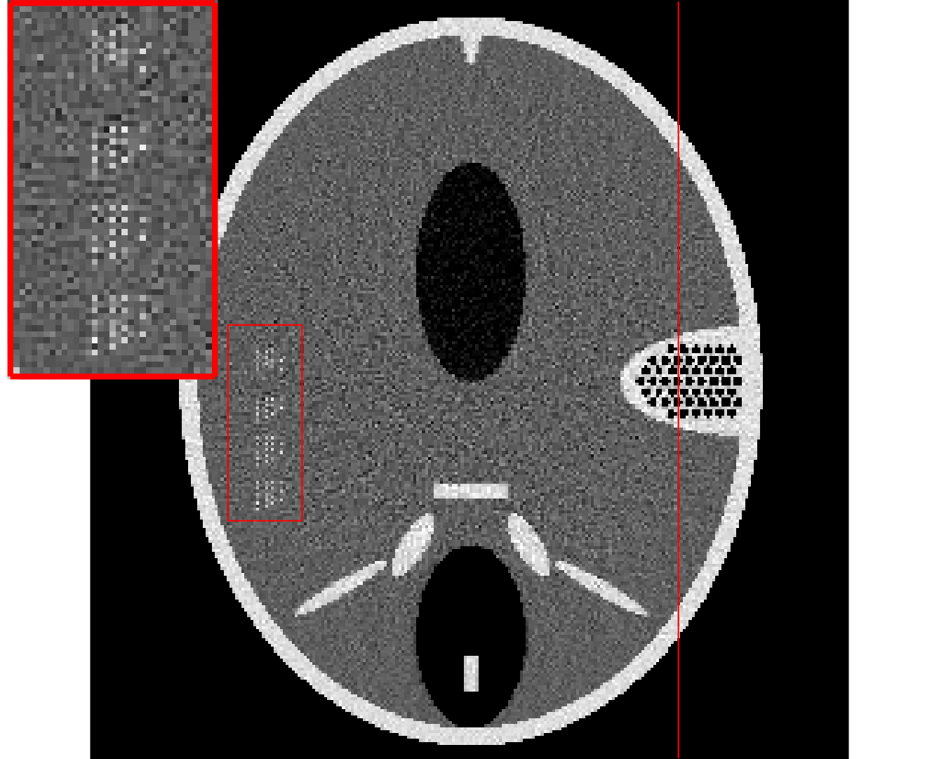
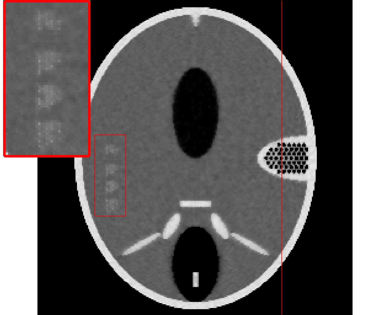
In this section, we show the performance of Lap-VARD by a phantom simulation experiment. We use the FORBILD head phantom with image size [17]. The original system matrix has dimension . The Haar wavelet transform with 3 levels is chosen and the corresponding transform matrix is . So the synthesized system matrix is . In this experiment, the photon intensity . We compare the performance of the Lap-VARD with the AM algorithm [16] and penalized AM algorithm with neighborhood penalty [18] and wavelet sparsity penalty [3]. The reconstructed images are shown in Fig. 1. The detail structures in the red boxes are magnified on the up-left corners.
Fig. 1(a) shows the ground truth of a FORBILD phantom. In (b), we plot the inverse wavelet transform of the posterior mean as the reconstructed image; and this image has both low noise and good resolution. The reconstruction of VARD [10] is shown in (c); while this image has low noise and good resolution, there are isolated salt-and-pepper noise pixels. Fig. (d) is the AM algorithm reconstruction. Because the Haar wavelet is orthogonal, the wavelet AM and the traditional AM are equivalent, and the result shows a high noise level. Fig. (e) and (f) are wavelet penalized AM algorithm reconstructions with penalty weights and . In (e), the penalty choice is too small and we can still see clear noise pixels. In (f), we have a proper choice of penalty weight and we have high smoothness and resolution at the same time. Fig (g) and (h) are neighborhood penalized AM reconstructions with penalty weights and . In (g), we have a proper penalty weight choice with a high resolution and a lower noise level; in (h), the penalty weight is too large and the detail structures are blurred.
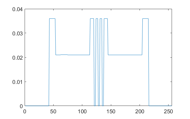
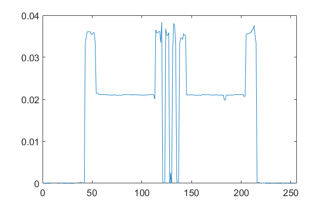
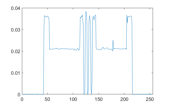
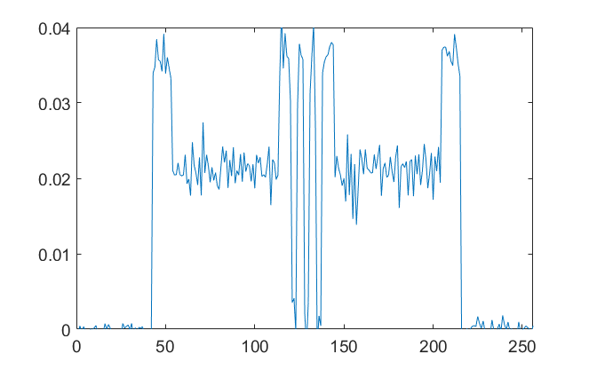
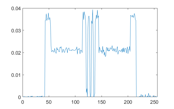
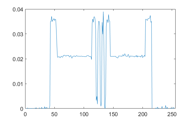
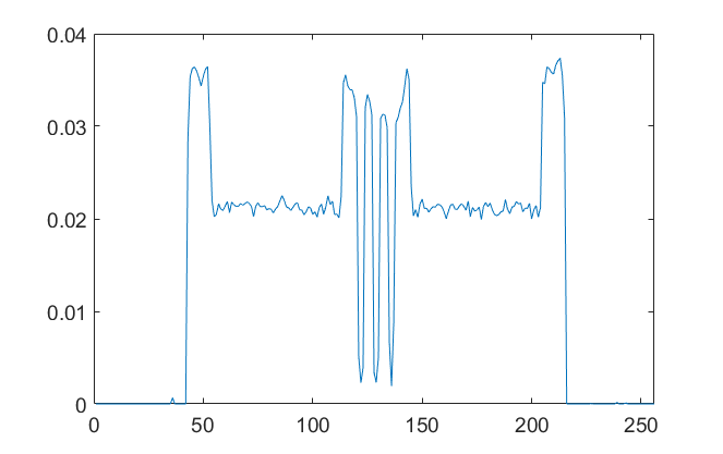
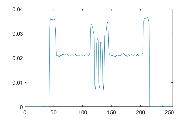
To further compare these algorithms rewording the smoothness and resolution performance, we plot the profiles of the vertical slice No. 199 which are highlighted with red line in Fig. 1. All these profiles are shown in Fig. 2. Fig 2(a) shows the ground truth of the profile. In (b), the reconstruction from the Lap-VARD is shown, we have quantitatively accurate reconstruction in both the flat area and peak-valley contrast. In (c), the profile from the original VARD is plotted, and we see similar performance as the Lap-VARD in smoothness restoration and peak-valley contrast, but we can also see salt-and-pepper noise pixels in VARD. The profile from unpenalized AM is shown in (d), we can see clear noise but the peak and valley contrast is kept. Fig (e) plots the result from wavelet penalized AM algorithm with penalty weight ; it still shows high noise compared with the Lap-VARD result which means the weight is insufficient. In (f), with a proper choice of penalty weight , the wavelet penalized AM result shows that even though it can generate an unbiased result, the noise level is comparatively higher than the Lap-VARD algorithm. Fig (g) is the neighborhood penalized AM result with penalty weight , and compared with the Lap-VARD result the noise level is too high. Another severe disadvantage is that the peak and valley values begin to shrink towards the average value. In an over-smoothed case, as shown in (h), with penalty weight raised to , the peak and valley contrast further shrinks and the result is quantitatively biased.
A quantitative error comparison is summarized in Table 1. The Lap-VARD outperforms all the other algorithms in root mean square error (RMSE) and peak signal-to-noise ratio (PSNR) performances.
| Lap-VARD | VARD | AM | wav-AM () | wav-AM() | AM() | AM() | |
| RMSE | 0.0020 | 0.0012 | 0.0010 | ||||
| PSNR(dB) | 38.37 | 35.42 | 26.74 | 32.70 | 34.93 | 31.79 | 29.88 |
From the simulation experiment above, we find that the Lap-VARD algorithm is able to derive a optional choice of penalty weight without sacrificing the smoothness or the resolution of reconstructed images.
IV conclusion
We introduced the Lap-VARD algorithm and implemented in X-ray computed tomography. The algorithm automatically generates the optimal wavelet penalty weight choice and the reconstructed image. Compared with a wavelet penalty weight which is from empirical experiments, the input data-driven Lap-VARD algorithm outperforms other algorithms in retaining the smoothness and detailed structure resolution. Compared with using a neighborhood penalty which loses resolution and generates biased results in a high peak and valley contrast scenario, the Lap-VARD is able to keep the contrast and generate an unbiased result.
Reference
- [1] W. A. Kalender, “X-ray computed tomography,” Physics in medicine and biology, vol. 51, no. 13, p. R29, 2006.
- [2] E. P. Simoncelli, “Modeling the joint statistics of images in the wavelet domain,” in SPIE’s International Symposium on Optical Science, Engineering, and Instrumentation. International Society for Optics and Photonics, 1999, pp. 188–195.
- [3] Q. Xu, A. Sawatzky, M. A. Anastasio, and C. O. Schirra, “Sparsity-regularized image reconstruction of decomposed k-edge data in spectral ct,” Physics in medicine and biology, vol. 59, no. 10, p. N65, 2014.
- [4] R. Baraniuk, “Compressive sensing [lecture notes],” IEEE Signal Process. Mag., vol. 24, no. 4, pp. 118–121, 2007. [Online]. Available: http://ieeexplore.ieee.org/stamp/stamp.jsp?arnumber=4286571
- [5] E. J. Candes, J. K. Romberg, and T. Tao, “Stable signal recovery from incomplete and inaccurate measurements,” Communications on pure and applied mathematics, vol. 59, no. 8, pp. 1207–1223, 2006.
- [6] R. Tibshirani, “Regression shrinkage and selection via the lasso,” Journal of the Royal Statistical Society. Series B (Methodological), pp. 267–288, 1996.
- [7] H. Zou, “The adaptive lasso and its oracle properties,” Journal of the American statistical association, vol. 101, no. 476, pp. 1418–1429, 2006.
- [8] T. J. Hebert and R. Leahy, “Statistic-based map image-reconstruction from poisson data using gibbs priors,” Signal Processing, IEEE Transactions on, vol. 40, no. 9, pp. 2290–2303, 1992.
- [9] D. P. Wipf and S. S. Nagarajan, “A new view of automatic relevance determination,” in Advances in neural information processing systems, 2008, pp. 1625–1632.
- [10] Y. Kaganovsky, S. Han, S. Degirmenci, D. G. Politte, D. J. Brady, J. A. O’Sullivan, and L. Carin, “Alternating minimization algorithm with automatic relevance determination for transmission tomography under poisson noise,” arXiv preprint arXiv:1412.8464, 2014.
- [11] J. A. Fessler, “Statistical image reconstruction methods for transmission tomography,” Handbook of medical imaging, vol. 2, pp. 1–70, 2000.
- [12] B. De Man, J. Nuyts, P. Dupont, G. Marchal, and P. Suetens, “An iterative maximum-likelihood polychromatic algorithm for ct,” IEEE transactions on medical imaging, vol. 20, no. 10, pp. 999–1008, 2001.
- [13] J. Lu, J. A. O’Sullivan, and D. G. Politte, “Wavelet regularized alternating minimization algorithm for low dose x-ray ct,” in Proceedings of The 14th International Meeting on Fully Three-Dimensional Image Reconstruction in Radiology and Nuclear Medicine, 2017, pp. 726–732.
- [14] R. M. Neal and G. E. Hinton, “A view of the em algorithm that justifies incremental, sparse, and other variants,” in Learning in graphical models. Springer, 1998, pp. 355–368.
- [15] S. Boyd and A. Mutapcic, “Subgradient methods,” Lecture notes of EE364b, Stanford University, Winter Quarter, vol. 2007, 2006.
- [16] J. A. O’Sullivan and J. Benac, “Alternating minimization algorithms for transmission tomography,” Medical Imaging, IEEE Transactions on, vol. 26, no. 3, pp. 283–297, 2007.
- [17] Z. Yu, F. Noo, F. Dennerlein, A. Wunderlich, G. Lauritsch, and J. Hornegger, “Simulation tools for two-dimensional experiments in x-ray computed tomography using the forbild head phantom,” Physics in medicine and biology, vol. 57, no. 13, p. N237, 2012.
- [18] J. D. Evans, D. G. Politte, B. R. Whiting, J. A. O’Sullivan, and J. F. Williamson, “Noise-resolution tradeoffs in x-ray ct imaging: A comparison of penalized alternating minimization and filtered backprojection algorithms,” Medical physics, vol. 38, no. 3, pp. 1444–1458, 2011.