On the Spatially Resolved Star-Formation History in M51 II: X-ray Binary Population Evolution

Abstract

We present a new technique for empirically calibrating how the X-ray luminosity function (XLF) of X-ray binary (XRB) populations evolves following a star-formation event. We first utilize detailed stellar population synthesis modeling of far-UV to far-IR photometry of the nearby face-on spiral galaxy M51 to construct maps of the star-formation histories (SFHs) on subgalactic ($\approx$400 pc) scales. Next, we use the $\approx$850 ks cumulative Chandra exposure of M51 to identify and isolate 2–7 keV detected point sources within the galaxy, and we use our SFH maps to recover the local properties of the stellar populations in which each X-ray source is located. We then divide the galaxy into various subregions based on their SFH properties (e.g., star-formation rate [SFR] per stellar mass [$M_{\star}$] and mass-weighted stellar age) and group the X-ray point sources according to the characteristics of the regions in which they are found. Finally, we construct and fit a parameterized XLF model that quantifies how the XLF shape and normalization evolves as a function of the XRB population age. Our best-fit model indicates the XRB XLF per unit stellar mass declines in normalization, by $\sim$3–3.5 dex, and steepens in slope from $\approx$10 Myr to $\approx$10 Gyr. We find that our technique recovers results from past studies of how XRB XLFs and XRB luminosity scaling relations vary with age and provides a self-consistent picture for how the XRB XLF evolves with age.

1. Introduction

For decades, it has been known that the X-ray luminosity from X-ray binaries (XRBs) in normal galaxies correlates with optical and far-IR luminosity (e.g., Fabbiano et al. 1982). This fact has led to several investigations evaluating the utility of X-ray emission as a probe of galaxy properties like star-formation rate (SFR) and stellar mass ($M_{\star}$) (see, e.g., Fabbiano 2006 for a review; Lehmer et al. 2010; Pereira-Santaella et al. 2011; Mineo et al. 2012a,b; Boroson et al. 2011; Zhang et al. 2012). The emission from the young ($\;\buildrel<\over{\sim}\;$100 Myr) high-mass XRB (HMXB; donor-star masses $\;\buildrel>\over{\sim}\;$2.5 $M_{\odot}$) population is thought to provide a relatively unobscured measure of SFR, a quantity that is difficult to determine well using measurements of the heavily-obscured UV light that is generated by the most massive, short-lived stars (e.g., Kennicutt & Evans 2012). In a complementary way, the emission from low-mass XRBs (LMXBs; donor-star masses $\;\buildrel<\over{\sim}\;$2.5 $M_{\odot}$) may provide an independent tracer of the star-formation history (SFH), or $M_{\star}$, due to LMXBs being associated with the older ($\;\buildrel>\over{\sim}\;$1 Gyr) stellar populations.

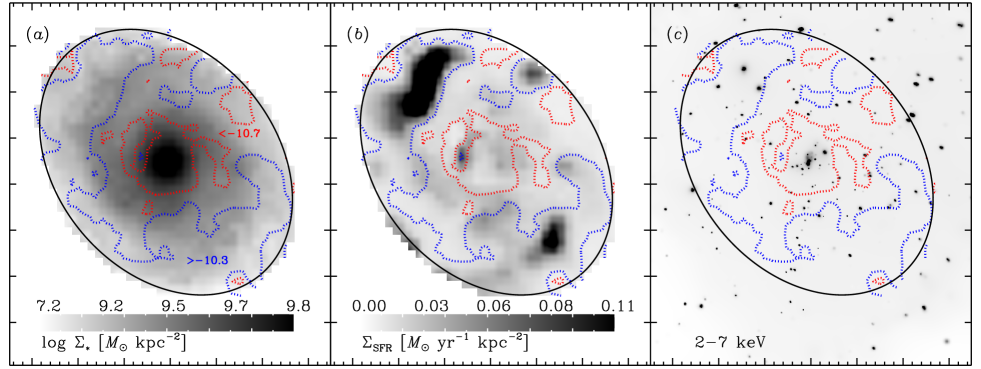
Figure 1.— Stellar mass ($M_{\star}$), star-formation rate (SFR), and adaptively-smoothed 2–7 keV Chandra images of NGC 5194 (M51). The black ellipse denotes the $K$-band galaxy size and orientation as derived by Jarrett et al. (2003), which we adopt throughout this paper. In each panel, we show contours that encircle regions with SFR/$M_{\star}>10^{-10.3}$ yr^-1 (blue dotted contours with “$>$$-10.3$” annotation) and SFR/$M_{\star}<10^{-10.7}$ yr^-1 (red dotted contours with “$<$$-10.7$” annotation). Regions between these two sets of contours have SFR/$M_{\star}=10^{-10.7}$ to $10^{-10.3}$ yr^-1. As expected high-sSFR regions enclose spiral arms, while low-sSFR regions are primarily located between spiral arms and in the galaxy bulge.

There are several obstacles to making XRB emission a well-utilized tracer of galaxy physical properties. For one, galaxies that are spatially unresolved in the X-ray band may suffer from considerable contamination from low-luminosity active galactic nuclei (AGN), which can have spectral properties consistent with XRBs. Furthermore, in nearby galaxies, where spatial resolution is sufficient to resolve the XRB population directly (e.g., Chandra observations of galaxies at $\;\buildrel<\over{\sim}\;$10–50 Mpc), it is currently not possible to separate confidently the HMXB and LMXB populations on a source-by-source basis, due to their similar X-ray spectral shapes and luminosities. Finally, the relatively shallow slope of the SFR-normalized HMXB X-ray luminosity function (XLF) leads to frustratingly large statistical variance in the integrated galaxy-wide X-ray luminosity ($\approx$0.2–0.3 dex; e.g., Gilfanov et al. 2004) making SF estimates highly uncertain.

Due to the above factors, reliable tracers of physical properties based on, e.g., far-UV–to–far-IR spectral energy distributions (SEDs), radio emission, nebular emission lines (e.g., H$\alpha$ and [O II]), and/or stellar absorption features (see, e.g., Madau & Dickinson 2014 for a recent review) are more commonly used than X-ray emission. However, it has recently become clear that there are several good reasons to continue to pursue studying and calibrating the relationships between XRB emission and physical properties, as XRBs can offer key discriminating information when utilized jointly with data from other wavelengths. For instance, XRBs provide a unique probe of the compact object population, which forms from remnants of $\lower 2.15277pt\hbox{$\;\buildrel>\over{\sim}\;$}8$ $M_{\odot}$ stars. As such, the XRB populations are uniquely sensitive to variations in the high-mass end of the initial mass function (IMF; see, e.g., Peacock et al. 2014, 2017; Coulter et al. 2017). Also, recent XRB population synthesis studies predict, and observational constraints appear to confirm, that the $L_{\rm X}$(HMXB)/SFR and $L_{\rm X}$(LMXB)/$M_{\star}$ scaling relations are significantly affected by variations in metallicity and parent stellar population age, respectively (e.g., Fragos et al. 2008, 2013a,b; Kim & Fabbiano 2010; Kaaret et al. 2011; Basu-Zych et al. 2013a, 2016; Brorby et al. 2014, 2016; Lehmer et al. 2014, 2016; Aird et al. 2017). These two quantities (metallicity and age) are similarly difficult to determine from stellar population synthesis and ISM fitting of optical/near-IR spectroscopic data, which are currently the most commonly used methods, and therefore could benefit from complementary and independent constraints from X-ray observations.

To advance the use of X-ray data as a means for constraining galaxy properties requires empirically calibrating how XRBs evolve with age for a variety of stellar birth properties (e.g., metallicity) and environmental conditions (e.g., local stellar densities). In this paper, we take a preliminary step in a long-term effort to develop such an empirical calibration by studying how XRB populations, as characterized by their XLF, vary with stellar age in the nearly face-on spiral galaxy M51. Our focus is to study XLFs of XRB populations that are not affected by extinction and confused by unrelated X-ray-emitting sources (e.g., hot gas and SN remnants). As such, we restrict our analyses to X-ray sources detected in the 2–7 keV bandpass, which encompasses only a fraction of the total number of X-ray sources detected in the full Chandra data set. A more thorough and complete characterization of all the sources detected in the rich M51 data set has been summarized in Kuntz et al. (2016), which we refer to throughout this paper.

In our procedure, we first utilize SED fitting of UV–to–far-IR photometric data to derive SFHs for small subregions of the galaxy. The details of this procedure were presented in part I of this series (Eufrasio et al. 2017), and here we make use of the SFH maps that resulted from this work (see salient features in $\S$2.1) We then construct a stellar-age dependent model of the XLF that describes the observed distribution of X-ray point sources, including estimates of completeness, contributions from potential background AGN, and the XRB populations we are modeling.

Throughout this paper, we assume a distance of 8.58 Mpc to M51 based on measurements of the tip of the red giant branch (McQuinn et al. 2016), which corresponds to an angular scale of 41.6 pc arcsec^-1. All X-ray fluxes are corrected for Galactic absorption, assuming a Galactic column density of $N_{\rm H}=1.5\times 10^{20}$ cm^-2 (Stark et al. 1992). Furthermore, throughout this paper we make estimates of quantities dependent on the initial mass functions (IMF), for which we employ the Kroupa (2001) IMF.

2. Data Analysis

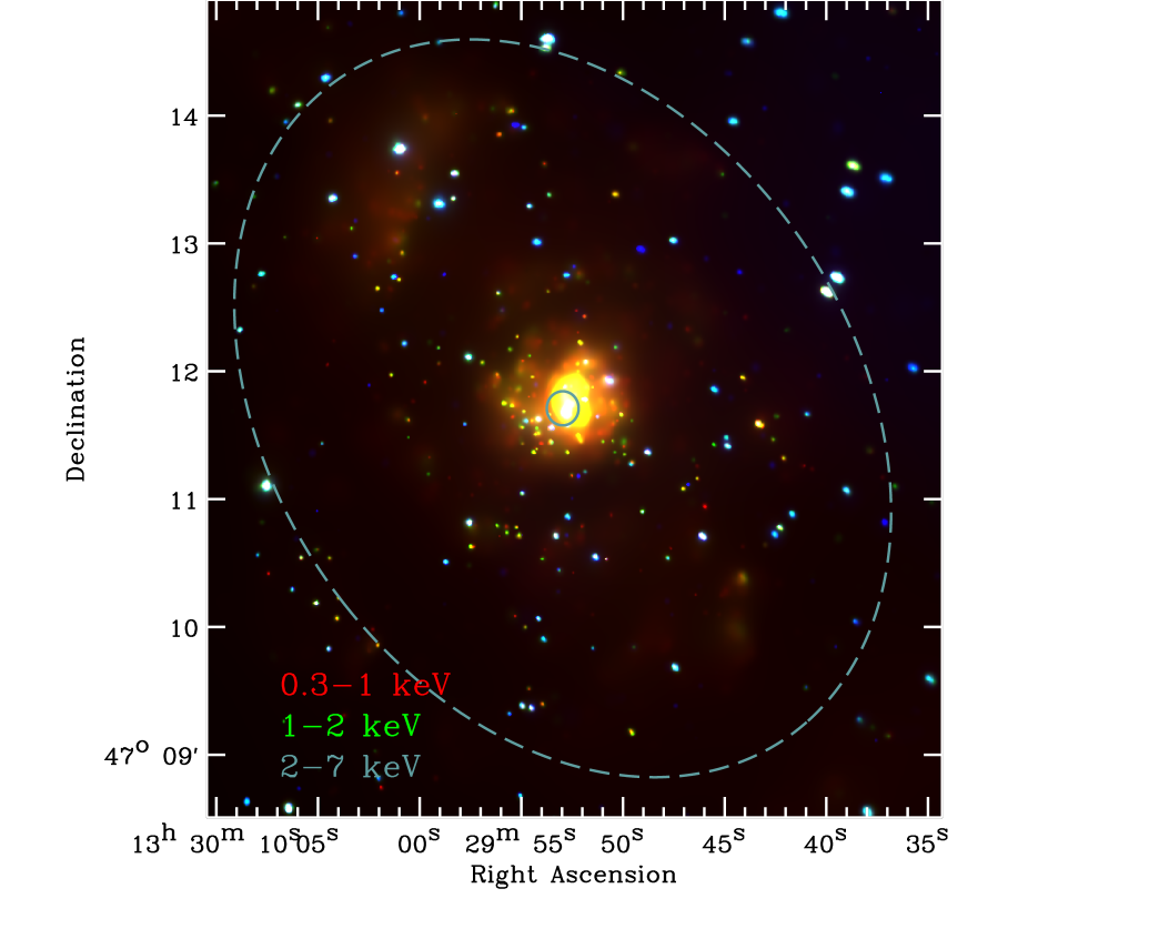
Figure 2.— Three-color Chandra image of M51. The image was constructed from 0.3–1 keV ($red$), 1–2 keV ($green$), and 2–7 keV ($blue$) exposure-corrected adaptively smoothed images. The dashed ellipse represents the total $K$-band galaxy size and orientation as described in $\S$2.1. Clear diffuse emission is evident in the softest band, following the central bulge and spiral arms. In our study of the XRB population, we limited our analyses to sources detected in the 2–7 keV band to avoid confusion with hot gas clumps and other unrelated soft point sources (e.g., SNe and remnants), and we excluded from consideration sources within a central circular region of radius 8 arcsec (blue circle) to avoid the AGN and confused sources.

Table 1Chandra Advanced CCD Imaging Spectrometer (ACIS) Observation Log for M51 (NGC 5194)

	Aim Point		Obs. Start	Exposure Timea	Flaringb	Flaring Timeb
Obs. ID	$\alpha_{\rm J2000}$	$\delta_{\rm J2000}$	(UT)	(ks)	Intervals	(ks)	Obs. Modec
354……………	13 29 49.9	+47 11 28	2000 Jun 20, 08:04	0014.8	…	…	F
1622	13 29 50.1	+47 11 27	2001 Jun 23, 18:47	0026.8	…	…	VF
3932	13 29 57.0	+47 10 39	2003 Aug 07, 14:32	0047.5	1	0.5	VF
12562	13 30 04.9	+47 09 54	2011 Jun 12, 06:52	0009.6	…	…	VF
12668	13 30 05.4	+47 09 53	2011 Jul 03, 10:32	0010.0	…	…	VF
13812	13 30 02.2	+47 10 49	2012 Sep 12, 18:25	0157.5	…	…	F
13813	13 30 02.2	+47 10 49	2012 Sep 09, 17:48	0178.7	1	0.5	F
13814d	13 30 03.8	+47 10 56	2012 Sep 20, 07:23	0189.8	…	…	F
13815	13 30 04.4	+47 11 00	2012 Sep 23, 08:13	0067.2	…	…	F
13816	13 30 04.4	+47 11 00	2012 Sep 26, 05:13	0073.1	…	…	F
15496	13 30 03.8	+47 10 56	2012 Sep 19, 09:21	0041.0	…	…	F
15553	13 30 05.9	+47 11 15	2012 Oct 10, 00:44	0037.6	…	…	F
Mergede	13 30 02.3	+47 10 54	…	853.6	2	1.0	…

Note.—Links to the data sets in this table have been provided in the electronic edition.
^a All observations were continuous. These times have been corrected for removed data that was affected by high background; see $\S$ 2.2.
^b Number of flaring intervals and their combined duration. These intervals were rejected from further analyses.
^c The observing mode (F=Faint mode; VF=Very Faint mode).
^d Indicates Obs. ID by which all other observations are reprojected to for alignment purposes. This Obs. ID was chosen for reprojection as it had the longest initial exposure time, before flaring intervals were removed.
^e Aim point represents exposure-time weighted value.

2.1. Spectral Energy Distribution Fitting and Property Map Creation

We determined subgalactic physical properties (e.g., SFR, $M_{\star}$, and SFH) within M51 following the procedure detailed in Eufrasio et al. (2017), part I of this series. For full details on this procedure and the data sets used, we refer the reader to that paper. Here we describe the salient features of our analyses and the resulting products that were used in this paper.

First, we utilized a large collection of far-UV–to–far-IR imaging data (including 16 total bands from GALEX, SDSS, 2MASS, Spitzer, and Herschel), convolved to a common spatial scale, to construct broad band SED maps. We chose to convolve all images with their respective point spread functions (PSFs) to a 25 arcsec FWHM spatial resolution. This is somewhat more coarse than the FWHM value of the Herschel SPIRE 250 $\mu$m channel, which is the lowest resolution imaging band used in our SED analyses. The data and resulting product maps were projected onto a grid with a pixel scale of 10 arcsec ($\approx$400 pc at our adopted distance).

Next, for each 10^′′ $\times$ 10^′′ pixel, we performed stellar population synthesis model fitting using PÉGASE (Fioc & Rocca-Volmerange 1997) and a SFH model that consisted of five discrete time steps, of constant SFR, at 0–10 Myr, 10–100 Myr, 0.1–1 Gyr, 1–5 Gyr, and 5–13.6 Gyr. The stellar emission from these specific age bins provide comparable bolometric contributions to the SED of a typical late-type galaxy SFH, and contain discriminating features that can be discerned in broad-band SED fitting (see Eufrasio et al. 2017 for details). In our procedure, we fit the SEDs for eight free parameters, including the normalizations (i.e., SFRs) of all five time steps, as well as three extinction values. Two of the extinction parameters describe the more heavily extincted population that is present in the “birth cloud” immediately following a star-formation event over the 0–10 Myr time frame and a single parameter is used to fit a more characteristic “diffuse” component applied to all populations. The resulting fits thus provide estimates for the SFH in each subgalactic pixel, which we used to construct the physical parameter maps. Here we chose to define the value of the SFR as the mean SFR over the last 100 Myr, which we derive using our SFH results. This allows us to make equivalent comparisons with SFR values provided in the literature (e.g., those derived from scaling relations like those in Kennicutt 1998 and Kennicutt & Evans 2012), which are often based on the same assumption.

In Figures 1$a$ and 1$b$, we show the stellar mass and SFR maps derived for M51 with contours of specific SFR (sSFR $\equiv$ SFR/$M_{\star}$) indicated. Throughout this paper, we restrict our analyses to the elliptical region defined by Mentuch-Cooper et al. (2010) for NGC 5194, which is estimated as an ellipse that traces a nearly constant stellar-mass density of 50 $M_{\odot}$ pc^-2. The ellipse has a semi-major axis of 191.5 arcsec, axis ratio of 0.75, and position angle of 50 deg east from north; we display the region as a black ellipse in each panel of Figure 1. As expected, the most intense star formation, as traced by the sSFR (enclosed by blue contours in Fig. 1), and the youngest stellar populations are found in the spiral arms, with less intense star formation and older stellar populations being located in the galactic bulge and in between the spiral arms. Going forward, we make use of these maps, along with the spatial locations of X-ray point source populations, to statistically constrain how XRB populations change with environment and evolve over time.

2.2. Chandra Data Reduction

All Chandra observations (hereafter, ObsIDs) were conducted using the S-array of the Advanced CCD Imaging Spectrometer (ACIS-S; see Table 1 for full observation log). Given the major-axis length of the M51 disk ($\approx$6.4 arcmin), the full galactic extent is covered by the single ACIS-S3 chip in nearly all 12 ObsIDs. For our data reduction, we made use of CIAO v. 4.8 with CALDB v. 4.7.1. We began by reprocessing the pipeline produced events lists, bringing level 1 to level 2 using the script chandra_repro. The chandra_repro script runs a variety of CIAO tools that identify and remove events from bad pixels and columns, and filter the events list to include only good time intervals without significant flares and non-cosmic ray events corresponding to the standard ASCA grade set (ASCA grades 0, 2, 3, 4, 6).

Using the reprocessed level 2 events lists for each ObsID, we generated preliminary 0.5–7 keV images and point-spread function (PSF) maps (using the tool mkpsfmap) with a monochromatic energy of 1.497 keV and an encircled counts fraction (ECF) set to 0.393. For each ObsID, we created preliminary source catalogs by searching 0.5–7 keV images with wavdetect (run including our PSF map), which was set at a false-positive probability threshold of $1\times 10^{-5}$ and run over seven wavelet scales from 1–8 pixels (1, $\sqrt{2}$, 2, 2$\sqrt{2}$, 4, 4$\sqrt{2}$, and 8). To measure sensitively whether any significant flares remained in our observations, we constructed point-source-excluded 0.5–8 keV background light curves for each ObsID with 500 s time bins. We found two 500 s intervals across all ObsIDs with flaring events of $\;\buildrel>\over{\sim}\;$3 $\sigma$ above the nominal background; these intervals were removed from further analyses and the resulting flare-free exposures are presented in Table 1.

For each ObsID, we used the preliminary source catalogs to register each flare-free aspect solution and events list to ObsID:13814, which had the longest exposure time. This process was carried out using CIAO tools reproject_aspect and reproject_events, respectively. The astrometric reprojections resulted in very small linear translations ($<$0.38 pixels; $<$0$\farcs$19), rotations ($<$0.1 deg), and stretches ($<$0.06% of the pixel size) for all ObsIDs. We created a merged events list, as well as a series of images in a variety of bands (including 0.3–1 keV, 1–2 keV, 0.5–2 keV, 2–7 keV, and 0.5–7 keV) and monochromatic exposure maps (at 1.497, 4.51, and 2.53 keV; in units of s cm²), using the CIAO script merge_obs. The merge_obs script properly projects all ObsID events lists and exposure maps to a common reference frame, and generates projected products for each ObsID that correspond to the merged products. We converted the exposure maps of each ObsID into vignetting-corrected exposure-time maps (in units of s) by dividing the exposure maps by the maximum effective area in that ObsID (see Hornschemeier et al. 2001 and Zezas et al. 2006 for additional details). These exposure-time maps were subsequently merged to form a merged vignetting-corrected exposure-time map. We further created 90% enclosed count-fraction PSF maps for each of the ObsIDs for an energy of 4.51 keV. We then created a vignetting-corrected exposure-time weighted merged PSF map, by summing the product of the PSF and exposure-time maps for each ObsID and dividing by the merged exposure-time map.

2.3. Main Catalog Creation and Properties

In Figure 2, we show a three-color (0.3–1 keV, 1–2 keV, and 2–7 keV) adaptively-smoothed image of M51, with the adopted elliptical boundary highlighted (see $\S$2.1 for details). Within the adopted galaxy boundaries, there are 208 significantly detected X-ray point sources (from the Kuntz et al. 2016 catalogs) and clear diffuse emission in the bulge region and along the spiral arms. A variety of X-ray point source types are present, including supernovae and remnants, XRBs, background AGN, and clumps of hot gas. Given that the goal of our study is to characterize the XRB populations, we limit ourselves to point sources detected in the 2–7 keV band (Fig. 1$c$). While this imposed limitation reduces the sensitivity of the Chandra survey to XRBs overall, it has the benefit of providing a cleaner sample of the XRB population by excluding “soft” unrelated sources like supernovae and remnants and hot gas clumps.

We constructed a point source catalog by searching the 2–7 keV image using wavdetect at a false-positive probability threshold of $1\times 10^{-6}$ over the $\sqrt{2}$ sequence (see above). We ran wavdetect using the timing map and 90% enclosed-count fraction PSF map, which resulted in a source catalog with properties (e.g., positions and counts) appropriate for point sources. We inspected all the images and source regions by eye to see if any additional source candidates were missed or confused. In particular, in the crowded nuclear regions of the galactic center, low-flux point sources may not be picked up by wavdetect due to the increased backgrounds. We found that point-source crowding in the central region was prohibitively large to obtain accurate point-source properties. As such, we excluded from further analyses a circular region at the center of the galaxy with an 8 arcsec radius. In total, 86 point sources were detected in the 2–7 keV band that were within the galactic footprint, yet outside the 8 arcsec radius central exclusion area. Hereafter, we exclusively utilize these sources and the adopted wavdetect catalog, which we define as our main catalog.

Given that we made use of the vignetting-corrected timing maps described above when running wavdetect, our main catalog contained measurements of the vignetting-corrected source count rates, which are background subtracted. In order to convert source 2–7 keV count rates to 2–10 keV fluxes, we used the CIAO script specextract to construct an exposure-weighted response matrix file (RMF) and ancillary response file (ARF) appropriate for a hypothetical source located at the exposure-weighted aim point. In xspec v. 12.8.2, we used the fakeit command to create a fake source with a power-law model that has Galactic absorption (see $\S$1) and photon-index $\Gamma=1.7$ and derived the count-rate to flux conversion factor for such a source. We utilized this same count-rate to flux conversion factor for all sources within our main catalog, since the detailed spectral shape of faint sources is uncertain for the majority of the sources in our catalog. Our adopted X-ray spectral model is broadly appropriate for the 2–10 keV emission from X-ray binaries across a variety of X-ray luminosities and describes well the overall spectral shapes of a variety of XRB-dominated nearby galaxies (e.g., Mineo et al. 2012; Lehmer et al. 2014, 2015). For the sources with $>$300 2–7 keV counts, we performed basic spectral fitting and found a mean photon index of $\Gamma=1.69$, albeit with a large scatter of $\sigma_{\Gamma}=0.54$. This translates into an estimated error on the luminosity of $\approx$17% due to the assumed SED, which is only somewhat larger than the $\approx$12% median error on photon statistics for all sources within M51.

The faintest sources in our main catalog have $\approx$6–10 net counts in the 2–7 keV band, which corresponds to a 2–10 keV flux limit of $\approx$(9–19) $\times 10^{-16}$ erg cm^-2 s^-1. At the distance of M51, these sources would have 2–10 keV luminosities of $\approx$(1.1–2.1) $\times 10^{36}$ erg s^-1. Hereafter, unless stated otherwise, we refer to X-ray luminosities $L_{\rm X}$ as pertaining to the 2–10 keV band.

We compared our main catalog sources with those provided in Kuntz et al. (2016). Out of the 86 sources in our catalog, we found matches to all but three sources: J132952.2+471100, J132954.3+471153, and J132943.4+471201. These three sources are faint, but clearly detected with 12–21 net counts in the 2–7 keV band. Kuntz et al. (2016) thoroughly searched multiple bands for source candidates, and eliminated several candidates based on their significance against the background and source extension, as derived by ACIS EXTRACT (Broos et al. 2012). Visual inspection of the lower-energy band images revealed that the three sources unique to our main catalog were located in regions with strong $\;\buildrel<\over{\sim}\;$1 keV emission from hot gas, and were thus likely to be rejected based on the extended emission from the nearby hot gas and the use of ACIS EXTRACT for evaluating source significance. For the remaining 83 sources, we found that 12 had classifications by Kuntz et al. (2016) based on broadband and H$\alpha$ HST imaging. Of these twelve sources, four were background galaxies, four were directly associated with star-forming regions, and six were coincident with H$\alpha$ bubbles. The latter six sources were noted to be a combination of transient and compact sources. Taken together, these classifications suggest that the majority of our sources are consistent with being XRBs. Our modeling techniques, discussed below, account statistically for potential background sources, which we estimate to be $\approx$6–10 over the footprint of M51, which suggests a reasonable fraction of the background sources may be identified by Kuntz et al. (2016). However, given the complex selection function of background sources through a face-on spiral galaxy like M51, we do not attempt to remove the few known background sources in our procedure below.

3. Analysis and Results

The primary goals of this paper are to (1) decompose the relative contributions of HMXBs and LMXBs to the total XRB luminosity by using subgalactic properties and (2) construct a comprehensive model for how the XRB XLF evolves as a function of age that agrees with empirical constraints on the observed XLF and subgalactic SFHs. In the sections below, we describe in detail our procedure for accomplishing these goals.

3.1. Completeness Estimates

To compute XLFs, we made use of the 2–7 keV catalog of 86 sources in the main catalog presented in $\S$2. Spatial variations in X-ray sensitivity, due to local background fluctuations, PSFs, effective exposures (e.g., chip gaps and bad pixels and columns), and source crowding, combined with incompleteness, can have significant effects on the shape of the observed XLF at X-ray luminosities within a factor of $\approx$10 of the detection limits. Therefore, these effects need to be properly characterized to compute the XLF.

In our analyses, we made use of the observed XLFs and models of the intrinsic XRB XLFs convolved with completeness functions that we derived from a Monte Carlo procedure. Our procedure was designed to provide the recovery fraction as a function of net source counts and source position. We began by constructing a series of 3,000 mock images. Each image consisted of our original 2–7 keV image plus 49 fake sources added to the image. Each source location was chosen to lie within the boundaries of a single box, with the fake images containing a grid of $7\times 7$ total boxes (defined in equal intervals of right ascension and declination). For a given image, only one source was placed in each box with a random location within that box. For each simulation, we pre-defined the total number of counts that would actually be registered on the detector, and created 200 mock images for 15 different choices of net counts (spanning 3–260 counts). The source counts were added to the fake images one at a time, with the distribution of photons following the average PSF shape, which we determined using the count distributions from bright sources within the image.

We note that the above procedure for creating fake images is somewhat different from standard procedures available through the marx ray-tracing code. We chose our approach because it very quickly allows us to construct many fake images with fake sources that contain an exact number of net counts that we define. We performed several curve-of-growth tests of the fake sources and verified that the count distributions from our approach are consistent with the PSFs of real sources in the image. Given the relatively small extent of M51, the PSF across the galactic footprint does not have significantly distorted shapes (i.e., non-circular), as is known to be the case for the Chandra PSF at large off-axis angles. As such, we caution that this approach will not likely work for sources with very large off-axis angles and distorted PSFs.

To construct completeness functions, we repeated the source detection procedure described in $\S$2 for all 3,000 mock images and compared mock catalogs with the input catalogs. In Figure 3, we show the fraction of fake sources recovered as a function of counts and angular distance from the M51 galactic center. We find the highest levels of completeness for regions near the center of the galaxy and only a mild decline in completeness in the outer regions of the galaxy $\approx$3 arcmin away from the galactic center. Such variations are expected due primarily to the larger average PSF size with galactocentric distance. In $\S$3.2 below, we describe how we use our completeness functions when measuring XRB XLFs.

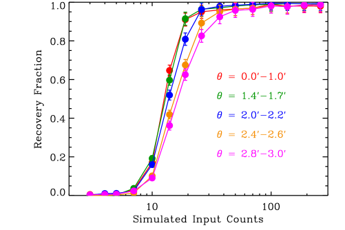
Figure 3.— Fraction of simulated sources recovered as a function of counts for five M51 galactocentric distances (see annotations). These recovery fraction curves show the highest completeness for sources near the center of the galaxy with declining completeness at larger galactocentric distances, where the average PSF is largest.

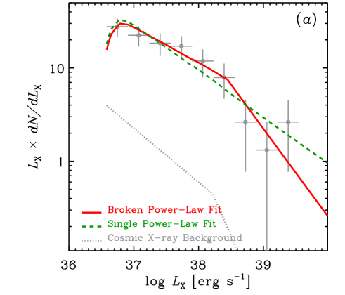
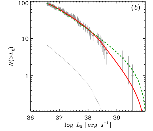
Figure 4.— Galaxy-wide differential ($a$) and cumulative ($b$) XLFs for X-ray point sources in M51 (gray filled circles with 1$\sigma$ Poisson errors). Note that the differential XLF plotted here is for display purposes, and does not show the finer binning used in fitting to the data. Best-fit models that include expected CXB sources plus XRBs, folded in with estimates of incompleteness (as described in $\S$3.2), have been shown for a broken power-law fit (solid red curves) and a single power-law fit (dashed green curves). The data are shown as gray circles with error bars, and have not been corrected for incompleteness and background sources. Incompleteness only affects the faintest source population below 2–10 keV luminosities of $L_{\rm X}\approx 10^{37}$ erg s^-1. Both the broken and single power-law models provide good fits to the data based on cstat.

3.2. Galaxy-Wide XRB XLF of M51

We began our XLF analyses by computing the galaxy-wide 2–10 keV XLF for M51. In Figure 4, we display the galaxy-wide observed XLF for M51 in both differential and cumulative form (gray filled circles with 1$\sigma$ Poisson error bars). These data contain completeness-uncorrected contributions from both XRBs in the disk of M51, as well as background X-ray point sources from the cosmic X-ray background (CXB; e.g., Kim et al. 2007; Georgakakis et al. 2008). In principle, there may also be X-ray point sources associated with foreground Galactic stars; however, inspection of optical counterparts to the X-ray sources, and characterizations provided by Kuntz et al. (2016), do not yield any Galactic stellar candidates.

We fit the observed galaxy-wide XLF following a forward-fitting approach, in which we include contributions from the XRBs and CXB sources, with incompleteness folded into our models. For the intrinsic XRB XLF, we attempted both single and broken power-law models of the respective forms:

$$\frac{dN}{dL_{\rm X,38}}=K_{s}\;f(L_{\rm X}),$$

$$\begin{split}f(L_{\rm X})\equiv\left\{\begin{array}[]{lr}L_{\rm X,38}^{-\gamma}&\;\;\;\;\;\;\;\;(L_{\rm X,38}<L_{c})\\ 0,&(L_{\rm X,38}\geq L_{c})\\ \end{array}\right.\end{split}$$ (1)

$$\frac{dN}{dL_{\rm X,38}}=K_{b}\;g(L_{\rm X}),$$

$$\begin{split}g(L_{\rm X})\equiv\left\{\begin{array}[]{lr}L_{\rm X,38}^{-\alpha_{1}}&(L_{\rm X,38}\leq L_{\rm b})\\ L_{\rm b}^{\alpha_{2}-\alpha_{1}}L_{\rm X,38}^{-\alpha_{2}},&\;\;\;\;(L_{\rm b}<L_{\rm X,38}<L_{c})\\ 0,&(L_{\rm X,38}\geq L_{c})\\ \end{array}\right.\end{split}$$ (2)

where $L_{\rm X,38}$ is the 2–10 keV X-ray luminosity in units of $10^{38}$ erg s^-1, $K_{s}$ and $K_{b}$ are normalization terms at $L_{\rm X,38}=1$ ($L_{\rm X}=10^{38}$ erg s^-1), $\gamma$ is the single power-law slope, and for the broken power-law, $\alpha_{1}$ is the faint-end slope, $L_{\rm b}$ is the break luminosity (in units of $10^{38}$ erg s^-1), and $\alpha_{2}$ is the bright-end slope. Both functions were terminated at a cut-off luminosity of $L_{c}=100$, which we adopted based on the literature (e.g., Mineo et al. 2012). In Equations (1) and (2) we also defined the functions $f(L_{\rm X})$ and $g(L_{\rm X})$ as short-hand for the $L_{\rm X}$-dependent portions of the single and broken power-laws, respectively.

For the CXB contribution, we utilized a fixed form from the number-counts estimates provided by Kim et al. (2007). The Kim et al. (2007) extragalactic number counts provide estimates of the number of sources per unit area versus 2–8 keV flux. The best-fit functions follow a broken power-law distribution with parameters derived from the combined Chandra Multiwavelength Project (ChaMP) and Chandra Deep Field-South (CDF-S) extragalactic survey data sets (see Table 4 of Kim et al. 2007). The number counts were converted to observed 2–10 keV XLF contributions by (1) multiplying the number counts by the areal extent of M51 as defined in $\S$2.1 (24.0 arcmin²); (2) converting CXB model fluxes to X-ray luminosities, given the distance to M51; and (3) multiplying the luminosities by a small correction factor to bring the 2–8 keV band luminosities to our adopted 2–10 keV band. The fixed CXB contribution is shown in Figure 4 as dotted curves; however, we note that these curves are not corrected for completeness (see below).

A complete model of the observed XLF, $dN/dL_{\rm X}({\rm obs})$, consists of the XRB intrinsic XLF component, $dN/dL_{\rm X}({\rm XRB})$, from Equation (1) or (2), plus the fixed CXB curve, $dN/dL_{\rm X}({\rm CXB})$, convolved with a galaxy-wide weighted completeness correction, $\xi(L_{\rm X})$, which was constructed using the radial-dependent completeness estimates calculated in $\S$3.1. $\xi(L_{\rm X})$ was thus calculated by statistically weighting the contributions from the model XLF at each annulus according to the observed distributions of X-ray point sources. Formally, we computed $\xi(L_{\rm X})$ using the following relation:

$$\xi(L_{\rm X})=\sum_{i}f_{\rm recov,i}(L_{\rm X})\times w_{i},$$ (3)

where $f_{\rm recov,i}(L_{\rm X})$ is the recovery-fraction curve for the $i$th annular bin (see Fig. 3) and $w_{i}$ is the fraction of total number of galaxy-wide sources within the $i$th annuluar bin based on the observed point-source distributions.

We thus modeled the observed XLF using a multiplicative model

$$dN/dL_{\rm X}({\rm obs})=\xi(L_{\rm X})[dN/dL_{\rm X}({\rm XRB})+dN/dL_{\rm X}({\rm CXB})].$$ (4)

In practice, we constructed the observed $dN/dL_{\rm X}({\rm obs})$ using a small constant bin of $\delta\log L_{\rm X}=0.036$ dex spanning the minimum luminosity of the subsample ($L_{\rm X}=2.8\times 10^{36}$ erg s^-1) to a maximum $L_{\rm X}=10^{40}$ erg s^-1. Therefore the majority of bins contained zero sources up to a maximum of three sources per bin. We evaluated the goodness of fit for our double power-law models using the Cash statistic (cstat; Cash 1979). Our single and broken power-law models contained two ($K_{s}$ and $\gamma$) and four ($K_{b}$, $\alpha_{1}$, $L_{b}$, and $\alpha_{2}$) free parameters, respectively (see Eqn. (1) and (2)). For the broken power-law model, we chose to constrain the break luminosity to the $L_{b}=$ 2–5 range to avoid confusion between solutions that place the break luminosity near either end of the luminosity range of the X-ray sources. This choice was based on visual inspection of the left panel of Figure 4 and is further motivated by observations in the literature of a break near the luminosity (see below).

Best-fit parameters for our models were determined by minimizing cstat. In this procedure, we found best fit solutions using custom software, which implemented a Monte Carlo chain of perturbing the variables randomly 10,000 times around successive best-fit solutions until convergence. We tested the convergence of this procedure by using very different combinations of initial parameter guesses, but found robust convergence in all tests. Once a best-fit solution was isolated, we constructed multi-dimensional grids of parameter values around the best-fit solutions and calculated the probability-density spaces in the vicinity of the best solutions. In Figure 4, we show the best-fitting observed galaxy-wide XLF models for the single (green curves) and broken (red curves) power-law fits in both the differential and cumulative form. The best-fit parameters, and their 1$\sigma$ confidence errors, are tabulated in Table 2.

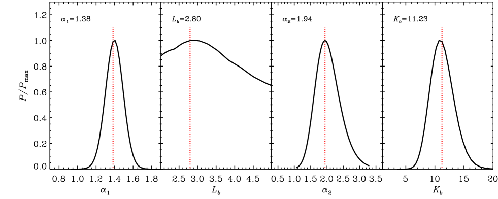
Figure 5.— Marginalized probability distribution functions for the broken power-law parameters that were fit to the galaxy-wide XLFs. The parameters include the faint-end power-law slope $\alpha_{1}$ ($a$), break luminosity $L_{b}$ ($b$), bright-end power-law slope $\alpha_{2}$ ($c$), and normalization to the XLF $K_{b}$ ($d$) (see Eqn. (2)). For reference, the best-fit values are highlighted with vertical red dotted lines.

We assessed the goodness of fit for our models by performing simulations. We constructed 50,000 simulated XLFs that are taken to be statistical “draws” from the best-fit XLF. For example, for the case of a single power-law, one of our simulated XLFs will be constructed by (1) perturbing the total number of X-ray point sources predicted from the model in a Poisson manner, and (2) assigning $L_{\rm X}$ values to the sources probabilistically following the best-fit XLF solution given in Table 2. For this set of simulated data, we then calculated the cstat value assuming the input model. The distribution of cstat values provides a measure of the probability of obtaining a given cstat value and allows us to assess whether a given data set is consistent with being drawn from the model. We find that both the single and broken power-law models provide good fits to the data, with the probability of obtaining the measured cstat values, or larger, being $P(\geq$cstat$)=$ 0.75 and 0.66, respectively. As such, a power-law break in the XLF is not formally required in the overall X-ray point-source population in M51.

In Figure 5, we show the marginalized probability density distribution functions for the broken power-law fit parameters $\alpha_{1}$, $L_{b}$, $\alpha_{2}$, and $K_{b}$ with the best-fit value annotated. All parameters, with the exception of $L_{b}$, are well constrained. $L_{b}$ itself shows a distinct maximum likelihood around $L_{b}\sim 2$ within the range of values explored. This value is consistent with high-luminosity breaks reported in the past (see, e.g., Sarazin et al. 2000; Gilfanov 2004; Kim & Fabbiano 2004; Zhang et al. 2012), and is often explained as being associated with a transition to almost exclusively black hole accretors, since the Eddington luminosity of a neutron star is near this limit. We did find that another peak of comparable, but somewhat lower probability around $L_{b}\sim 0.2$ when allowing $L_{b}$ to vary outside of this range, and this solution likely represents an additional real break, which has been reported in past studies as well (e.g., Gilfanov 2004; Voss & Gilfanov 2006; Voss et al. 2009; Zhang et al. 2012). The nature of this break is more mysterious, but may be associated with a reduction in XRBs with main sequence donor stars at lower luminosities and the onset of XRBs with red-giant donors at higher luminosities (e.g., Fragos et al. 2008).

3.3. LMXB and HMXB XLF Decomposition

As with most spiral galaxies, the stellar populations within M51 span a wide range of stellar ages due to a sustained SFH spanning several Gyr. In the case of M51, the most active episodes of star formation occurred more than 100 Myr ago, with the most active growth occuring over the 0.1–5 Gyr time frame (see, e.g., Eufrasio et al. 2017 and references therein). Inevitably, the XRB population within M51, and late-type galaxies in general, will contain both LMXB and HMXB populations. Although there have been several investigations of the stellar-mass scaling of LMXB XLFs using elliptical galaxies (e.g., Gilfanov 2004; Zhang et al. 2012; Lehmer et al. 2014; Peacock et al. 2014, 2017) and the SFR scaling of HMXB XLFs based on spirals (e.g., Grimm et al. 2002; Mineo et al. 2012), these studies assume that either LMXBs or HMXBs dominate the observed XRB populations. However, there are reasons to believe that such assumptions are unlikely to be fully correct. For example, XRB population synthesis models predict that the LMXB XLF normalization declines significantly with increasing stellar population age (e.g., Fragos et al. 2008), suggesting that stellar-mass scaled LMXBs based on elliptical galaxies alone are likely to underpredict the LMXB XLF in young galaxies. Some evidence for this has already been apparent in the LMXB populations of ellipticals with varying mean stellar ages (see Kim et al. 2009; Lehmer et al. 2014), and there is some suggestion that the younger mean stellar population within M51 itself may be influencing the LMXB XLF (see Kuntz et al. 2016 and below).

In this section, we make use of the $M_{\star}$ and SFR maps presented in Figure 1 (see Eufrasio et al. 2017 for details) as a means for probabilistically separating, respectively, LMXB and HMXB contributions to the XLF. Our strategy assumes that the normalizations (not the shapes) of the LMXB and HMXB XLFs scale with $M_{\star}$ and SFR, respectively, on scales down to $\sim$1–2 kpc. Such an assumption may not be fully accurate, in particular, due to the influence of XRB natal kicks, in which SNe that precede the formation of the compact object within the XRB can lead to a strong peculiar velocity ($\sim$100–200 km s^-1) of the binary system relative to its birth population (e.g., Brandt & Podsiadlowski 1995). Thus far, empirical studies indeed show that these natal kicks are likely to have some influence on the distribution and velocities of LMXBs in the Milky Way relative to their parent stellar populations (e.g., Podsiadlowski et al. 2005; Repetto et al. 2012, 2017; Maccarone et al. 2014). However, such kicks are estimated to scatter only a fractionally small number of systems relative to their parent stellar population on the subgalactic scales that we probe here (typically $\sim$2 kpc), as evidenced by only a small excess of sources found outside of elliptical galaxies and the observation that scaling relations appear to hold on local scales (e.g., Kundu et al. 2007; Zhang et al. 2013; Mineo et al. 2014). For young HMXBs, the typical center-of-mass velocity of $\;\buildrel<\over{\sim}\;$30 km s^-1 is not enough to significantly displace these objects from their parent population over the binary lifetimes (see Antoniou & Zezas 2016). For LMXBs, the spatial distribution of the stellar populations from which they are born are smoothed out by the galaxy velocity field, in the same way as the LMXBs themselves. Therefore, the LMXBs are sampling the same average old stellar populations. To this extent, we expect that XRBs found in areas with the highest sSFR will have the largest likelihood of being HMXBs, while those in the lowest sSFR will have the highest likelihood of being LMXBs. The probability of the X-ray source being a background X-ray source from the CXB is estimated following the number counts and the areas enclosed by a given sSFR range (see $\S$3.2 for details).

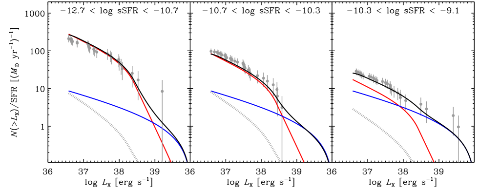
Figure 6.— SFR-normalized XLFs for three subregions of M51 that have been separated by sSFR (see annotations at the tops of each panel). As per Fig. 4, gray filled circles with error bars are the measured XLFs without corrections and the dotted curves represent the estimated CXB contributions. There is clear evidence that the observed XLF both declines in normalization and flattens in shape going from low-sSFR to high-sSFR. Our best-fit decomposition model, which is based on a stellar-mass scaled LMXB XLF (red curves) and a SFR scaled HMXB XLF (blue curves), is plotted in each panel. We note that since the y-axis is normalized by SFR, the HMXB model is the same in each of the three panels.

We therefore constructed a decomposition XLF model that contained all of the above elements. For each of the X-ray point sources, we identified local estimates of the $M_{\star}$ and SFR from our maps, and computed the sSFR associated with that X-ray source location (i.e., the sSFR within a $\approx$400 pc region around the X-ray source). We then sorted the X-ray point source catalog by local sSFR and broke up the sample into 28 sSFR bins (three X-ray sources per sSFR bin) that progressed from lowest to highest sSFR. For each of the sSFR bins, we computed the total areal extent across M51 that contained sSFR values within the range defined by the bin, and estimated the number of CXB sources expected over this area (see $\S$3.2). Following Equation (2), we computed the X-ray point source completeness function, $\xi({\rm sSFR}_{i},L_{\rm X})$, for each of the 28 sSFR bins ($i\equiv$ $1\ldots 28$).

To construct a decomposition XLF model, we used the past results from Zhang et al. (2012) and Mineo et al. (2012) as guidance on the basic forms of the LMXB and HMXB XLFs, respectively. From Zhang et al. (2012), the LMXB XLF within massive ellipticals exhibits two breaks located at $\approx$$2\times 10^{37}$ erg s^-1 and $\approx$$2.5\times 10^{38}$ erg s^-1 in the 2–10 keV band adopted here. These breaks are consistent with our findings for the galaxy-wide XLF studied in $\S$3.2 above (see also Fig 4). We therefore modeled the LMXB XLF as a power-law with two breaks fixed at these values, but with a normalization that scales with stellar mass. The two-break power law model has the form:

$$\begin{split}h(L_{\rm X})\equiv\left\{\begin{array}[]{lr}L_{\rm X,38}^{-\alpha_{1}}&(L_{\rm X,38}\leq L_{\rm b,1})\\ L_{\rm b,1}^{\alpha_{2}-\alpha_{1}}L_{\rm X,38}^{-\alpha_{2}},&\;\;\;\;(L_{\rm b,1}<L_{\rm X,38}\leq L_{b,2})\\ L_{\rm b,1}^{\alpha_{2}-\alpha_{1}}L_{\rm b,2}^{\alpha_{3}-\alpha_{2}}L_{\rm X,38}^{-\alpha_{3}},&\;\;\;\;(L_{\rm b,2}<L_{\rm X,38}\leq L_{c})\\ 0.&(L_{\rm X,38}>L_{c})\\ \end{array}\right.\end{split}$$ (5)

From Mineo et al. (2012), galaxies with sSFR $\lower 2.15277pt\hbox{$\;\buildrel>\over{\sim}\;$}10^{-10}$ yr^-1 (i.e., for the inferred HMXB population) have XLFs that are more consistent with a single power-law going out to $L_{\rm X}\approx$ (1–10) $\times 10^{40}$ erg s^-1. Thus, we chose to model the XLF as a single power-law (i.e., $f(L_{\rm X})$ defined in Eqn. (1)), with a normalization that scales with SFR and a cut-off at $10^{40}$ erg s^-1.

In relation to the 28 sSFR bins defined above, we expect that the XLF shape should go from looking more like a broken power law at low-sSFR to more like a single power law at high-sSFR. Since we have constructed each sSFR bin to include only three X-ray sources, and expect at least some of these sources to be background sources, it is not easy to visually see such an effect. However, a broader binning of the data into three sSFR bins clearly reveals such a trend. In Figure 6, we show the total observed XLFs for three sSFR bins, normalized by the SFR appropriate for each bin (i.e., the total SFR across the galactic extent from regions within a given sSFR bin). As expected, we indeed see the most obvious indication of a break in the lowest-sSFR bin, a trend that has been indirectly observed since early Chandra XLF studies of various nearby galaxies and subgalactic regions (e.g., bulges, spiral arms, and interarm regions; e.g., Kilgard et al. 2002, 2005; Trudolyubov et al. 2002; Kong et al. 2003; Soria & Wu 2003). We also see that the SFR-normalized XLF reaches the largest number of X-ray sources per SFR in the lowest-sSFR bin. If all X-ray sources throughout the galaxy were HMXBs, we would expect the SFR-normalized XLF to be roughly the same in each panel. The increased normalization towards low-sSFR is a direct indication of a corresponding increase in the number of LMXBs per unit SFR for low sSFR.

Table 2Summary of Fits to X-ray Luminosity Functions

Model Description	Parameter	Param Value	Units
Galaxy-Wide Power-law Models
single power law	$K_{s}$	9.3${}^{+1.2}_{-1.4}$
	$\gamma$	1.49${}^{+0.06}_{-0.08}$
	cstat	194.0
	$P(\geq$cstat$)$	0.75
broken power law …………	$K_{b}$	11.2${}^{+1.4}_{-2.4}$
	$\alpha_{1}$	1.38${}^{+0.09}_{-0.10}$
	$\alpha_{2}$	1.94${}^{+0.38}_{-0.34}$
	$L_{b}$	2.80${}^{+1.59}_{-0.39}$	$10^{38}$ erg s-1
	cstat	191.5
	$P(\geq$cstat$)$	0.66
LMXB and HMXB Decomposition Model
LMXB component	$K_{\rm LMXB}$	27.89${}^{+67.33}_{-10.04}$	($10^{11}$ $M_{\odot}$)-1
	$\alpha_{1}$	1.44${}^{+0.03}_{-0.62}$
	$L_{b,1}$	0.2†	$10^{38}$ erg s-1
	$\alpha_{2}$	1.32${}^{+0.28}_{-0.14}$
	$L_{b,2}$	2.5†	$10^{38}$ erg s-1
	$\alpha_{3}$	3.0†
HMXB component	$K_{\rm HMXB}$	1.10${}^{+0.83}_{-0.71}$	($M_{\odot}$ yr-1)-1
	$\gamma$	1.24${}^{+0.25}_{-0.23}$
	$C_{\rm global}$	710.3
	$P(\geq C_{\rm global}$)	0.13
Star-Formation History Model
	$K_{0}$	52${}^{+24}_{-15}$	($10^{11}$ $M_{\odot}$)-1
	$\kappa$	0.51${}^{+0.42}_{-0.27}$
	$\alpha_{1}$	1.42${}^{+0.06}_{-0.21}$
	$L_{b,1}$	0.2†	$10^{38}$ erg s-1
	$\alpha_{2}({\rm 10~{}Gyr})$	1.37${}^{+2.20}_{-0.46}$
	$L_{b,2}$	2.5†	$10^{38}$ erg s-1
	$\alpha_{3}({\rm 10~{}Gyr})$	3.0†
	$C_{\rm global}$	748.5
	$P(\geq C_{\rm global}$)	0.10

^†Indicates parameter was fixed in fitting procedure (see text for details).

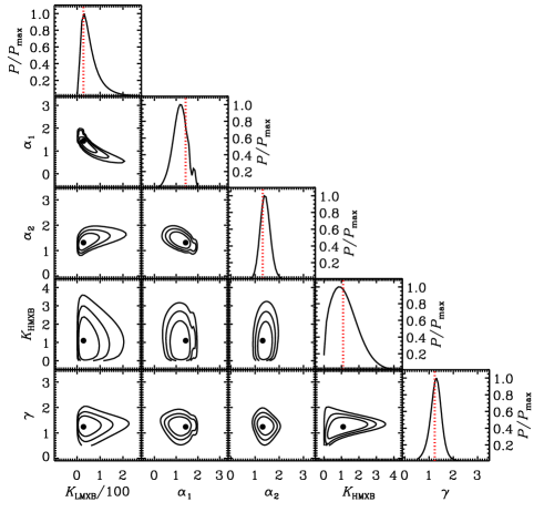
Figure 7.— Marginalized best-fit parameter estimate contours for pairs of parameters (contour plots with 68%, 87%, and 95% confidence contours drawn) and probability density distributions for single parameters (continous curves), pertaining to the decomposition model described in $\S$3.3. The global best-fit parameter values are indicated in each of the contour plots with a single black filled circle and vertical red dotted lines in the probability density distribution diagrams. All parameters in our model are well constrained, albeit with large fractional uncertainties for some parameters.

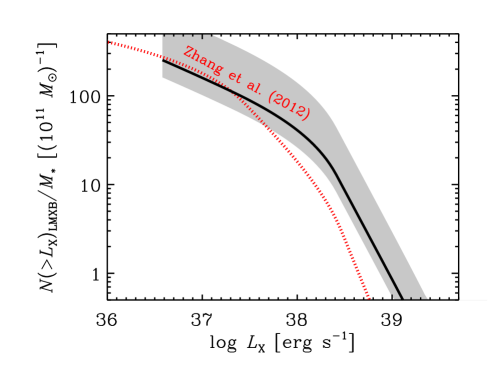
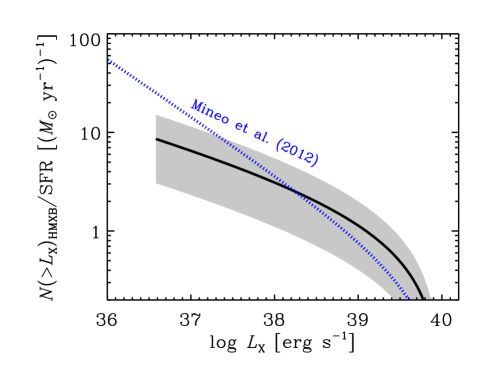
Figure 8.— Our best-fit stellar-mass normalized LMXB XLF model ($a$) and SFR normalized HMXB XLF model ($b$) (solid black curves). For comparison, we have overlayed, with dotted curves, the elliptical-galaxy based LMXB XLF derived by Zhang et al. (2012) and the high-sSFR late-type galaxy based HMXB XLF derived by Mineo et al. (2012). Our recovered LMXB and HMXB XLFs for M51 appear broadly consistent with those from the literature with some key differences, likely due to differences in GC populations, SFHs, metallicities, and assumptions between analyses (see detailed discussion in $\S$3.3).

Using the full set of 28 sSFR bins, for the $i$th bin we constructed the following scaled model for the overall observed XLF:

$$\begin{split}dN/dL_{\rm X}({\rm sSFR}_{i})=\xi({\rm sSFR}_{i},L_{\rm X})[{\rm SFR}_{i}K_{\rm HMXB}f(L_{\rm X})+\\ M_{\star,i}K_{\rm LMXB}h(L_{\rm X})+dN/dL_{\rm X}({\rm sSFR}_{i},{\rm CXB})],\end{split}$$ (6)

where $f(L_{\rm X})$ and $h(L_{\rm X})$ are the un-normalized single and double-break broken power-law functions (see Eqn. (1) and (5)) and $K_{\rm LMXB}$ and $K_{\rm HMXB}$ are the corresponding $M_{\star}$ and SFR scaled XLF normalizations, respectively. This model contains five parameters: $K_{\rm HMXB}$ and $\gamma$ for the SFR-scaled HMXB XLF and $K_{\rm LMXB}$, $\alpha_{1}$, and $\alpha_{2}$ for the $M_{\star}$-scaled LMXB XLF. Since $\alpha_{3}$ describes the $L_{\rm X}\lower 2.15277pt\hbox{$\;\buildrel>\over{\sim}\;$}2.5\times 10^{38}$ erg s^-1 slope, and few sources are present, we could not constrain its value. We chose to fix its value at $\alpha_{3}=3.0$, a value consistent with field LMXBs in elliptical galaxies (see extended discussion in $\S$3.3 and Peacock et al. 2017 for motivation).

To determine best-fit parameters, we made use of a summed cstat value to obtain a global statistic, $C_{\rm global}$, following

$$C_{\rm global}=\sum_{i=1}^{28}C({\rm sSFR}_{i}),$$ (7)

where $C({\rm sSFR}_{i})$ is the cstat value for the $i^{\rm th}$ sSFR bin. Our model was thus fit by minimizing $C_{\rm global}$ following the procedure that we developed in $\S$3.2. The best fit parameters for our LMXB and HMXB decomposition model are summarized in Table 2.

In Figure 6, we show the SFR-normalized best-fit model XLFs (in cumulative form) for the three sSFR bins discussed above with HMXB (blue curves) and LMXB (red curves) contributions indicated. By construction, our SFR-normalized HMXB XLF model is the same in each of the panels of Figure 6; however, the contribution from the LMXB XLF model grows with decreasing sSFR. This simple model provides a reasonable characterization of the basic scaling of the XLFs in all three panels. We re-iterate that our model is a single model that contains an HMXB XLF with normalization $K_{\rm HMXB}$ that scaled linearly with SFR and an LMXB component with normalization $K_{\rm LMXB}$ that scales linearly with $M_{\star}$. Only SFR and $M_{\star}$ vary between each of the three panels in Figure 6.

We performed goodness-of-fit simulations, as described in $\S$3.2, and found $P(\geq C_{\rm global})=0.13$, suggesting that the data are marginally consistent with the adopted model. In Figure 7, we show the marginalized probability density functions and contours for parameter pairs. All parameters in the model are constrained by the data, albeit with large fractional uncertainties for some of the parameters. For example, the normalization terms are not well constrained, primarily due to the correlation between the LMXB normalization, $K_{\rm LMXB}$, and its slopes, $\alpha_{1}$ and $\alpha_{2}$.

In Figure 8, we show the decomposed LMXB and HMXB XLFs normalized by $M_{\star}$ and SFR, respectively, and display the best models derived by Zhang et al. (2012; LMXBs) and Mineo et al. (2012; HMXBs), for comparison. We find reasonable agreement between our derived LMXB and HXMB XLFs in M51 and those found for large populations of galaxies, with some differences. The equivalent elliptical galaxy LMXB XLF slopes from Zhang et al. (2012) are $\alpha_{1}=1.02^{+0.07}_{-0.08}$, $\alpha_{2}=2.06^{+0.06}_{-0.05}$, and $\alpha_{3}=3.63^{+0.67}_{-0.49}$. Our LMXB XLF shows a somewhat shallower value of $\alpha_{2}=1.32^{+0.28}_{-0.14}$, but is otherwise consistent with the slopes from Zhang et al. (2012). For the HMXBs, we find a marginally shallower XLF slope of $\gamma=1.24^{+0.25}_{-0.23}$ compared with the $\gamma=1.58\pm 0.02$ value obtained by Mineo et al. (2012) for high-sSFR galaxies; however, the HMXB XLFs appear to be consistent at least for $L_{\rm X}\lower 2.15277pt\hbox{$\;\buildrel>\over{\sim}\;$}3\times 10^{37}$ erg s^-1, where the constraints are best.

The near consistency between our recovered LMXB and HMXB XLFs with those in the literature is encouraging, and there are a number of factors that could explain any residual differences. For example, the LMXB XLF derived by Zhang et al. (2012) was based primarily on massive elliptical galaxies, which have a larger number of globular clusters (GCs) per unit stellar mass than late-type galaxies like M51. Due to their high stellar densities and enhanced stellar interaction rates over stellar systems in the galactic field, GCs contain significant numbers of LMXBs that form via dynamical interactions (see, e.g., Benacquista & Downing 2013 for a review). As such, we would expect there to be more GC LMXBs per unit galactic stellar mass for ellipticals over M51, and thus an elevated LMXB XLF from the Zhang et al. (2012) study. However, there are also indications that the stellar-mass normalized field LMXB XLF is larger for younger stellar populations (e.g., Kim et al. 2010; Lehmer et al. 2014), which would presumably favor an enhanced stellar-mass normalized field LMXB XLF in M51 over that of typical ellipticals, which have older SFHs. It is possible that the combination of these effects has led to similar LMXB XLFs for M51 and typical ellipticals.

Figure 9.— Galaxy-wide cumulative XLF for M51 (gray circles with error bars; same as Fig. 4$b$), with our best LMXB (red curve) and HMXB (blue curve) decomposition model overlayed. As per Fig. 4, the dotted curve represents the estimated CXB contribution. The decomposition model was constructed by multiplying the galaxy-wide stellar mass and SFR by the respective LMXB and HMXB model terms provided in equation (6). We infer that HMXBs dominate the cumulative XLF for M51 above $L_{\rm X}\approx$ (3–5) $\times 10^{38}$ erg s^-1, with LMXBs dominating at lower luminosities. The integrated XLFs suggest that LMXBs and HMXBs provide similar contributions to the overall integrated X-ray power output of the galaxy.

The HMXB XLF from Mineo et al. (2012) was constructed for a sample of galaxies with sSFR $\lower 2.15277pt\hbox{$\;\buildrel>\over{\sim}\;$}10^{-10}$ yr^-1 and in some galaxies, like M51, the bulge regions were excluded in an effort to isolate the HMXB population. In their analyses, however, they assumed that the LMXB contributions in the disk regions was negligible and did not make any corrections for this population. In our analysis, we found that our best models predict at least some contribution from LMXBs even in the highest-sSFR regions. In the far-right panel of Figure 6, we show the decomposed XLF for the highest sSFR regions in M51. Our best model suggests that the steeper LMXB component of that model is comparable to the HMXBs at $L_{\rm X}\lower 2.15277pt\hbox{$\;\buildrel<\over{\sim}\;$}10^{38}$ erg s^-1, and taken together, the LMXB plus HMXB XLF takes on a steeper slope that is more consistent with the Mineo et al. (2012) XLF. It is therefore plausible that the true HMXB XLF is flatter than previously reported (as seen in the right panel of Fig. 8), and past investigations may not be accounting for an important LMXB contribution at low $L_{\rm X}$. However, further studies of additional galaxies would be needed to verify this claim. M51 has a unique SFH and history of abundance enrichment that may not be representative of galaxies as a whole. These properties (i.e., SFH and metallicity) are known to influence the formation of XRBs (see, e.g., Fragos et al. 2013).

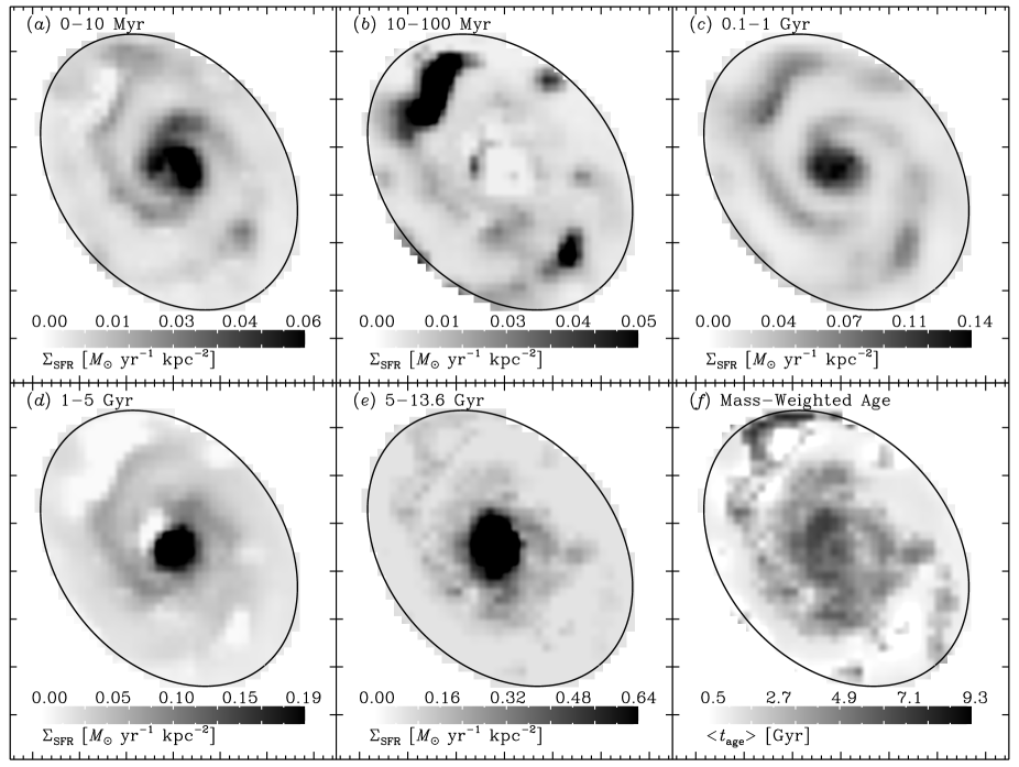
Figure 10.— SFH maps of M51 in five stellar-age bins: 0–10 Myr, 10–100 Myr, 0.1–1 Gyr, 1–5 Gyr, and 5–13.6 Gyr (see annotations). The scales of these images are linear and vary between frames to highlight the spatial distributions of the star-formation activity within each stellar-age range. The bottom-right frame shows the spatial distribution of the mass-weighted mean stellar age, $\langle t_{\rm age}\rangle$, a quantity we use to separate regions of different SFHs (see $\S$3.4 for details).

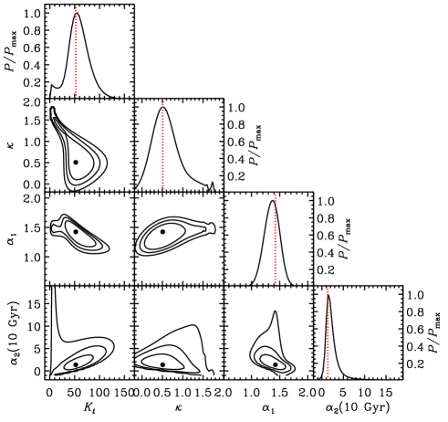
Figure 11.— Same as Figure 7, but for parameters involved in the SFH XLF decomposition model described in $\S$3.4.

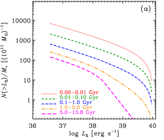
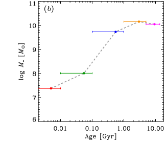
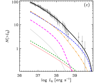
Figure 12.— ($a$) Best-fit SFH XLF decomposition model showing how the XRB XLF evolves with stellar age. Each curve shows the XLF for a population of XRBs within the designated age range, normalized by the stellar mass of that same age range. Our model indicates that the stellar-mass normalized XRB XLF declines in normalization by $\sim$3–3.5 orders of magnitude and the overall XLF slopes steepen significantly between $\sim$0–10 Myr and $\sim$5–13.6 Gyr. ($b$) Integrated galaxy-wide SFH for M51, expressed in terms of the current stellar mass contributions from the five stellar age bins. The bins have been color coded to match those defined in panel $a$. The majority of the stellar mass in M51 is attributed to the 1–5 Gyr population. ($c$) Galaxy-wide cumulative XLF for M51 (gray circles with error bars; same as Fig. 4$b$). As per Fig. 4, the dotted curve represents the estimated CXB contribution. Our SFH XLF model (panel $a$), folded in with the SFH of M51 (panel $b$), is shown as a black curve with contributions from each of the five stellar age bins indicated with colored curves, which have the same meaning as they did in panel $a$. Our SFH model provides an excellent characterization of the galaxy-wide XLF of M51 and contains the same number of fitting parameters as the broken power-law model.

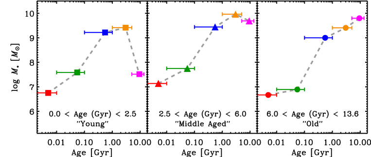
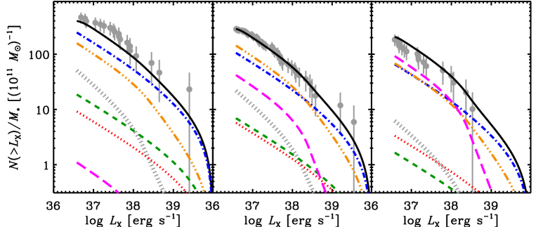
Figure 13.— (Top Panels) Five-step SFHs for three subgalactic regions that were selected by mass-weighted mean stellar ages, with the ranges annotated in the lower portion of each panel. Here we divided M51 into “young” ($\langle t_{\rm age}\rangle=$ 0–2.5 Gyr; left panel), “middle aged” ($\langle t_{\rm age}\rangle=$ 2.5–6 Gyr; middle panel), and “old” ($\langle t_{\rm age}\rangle=$ 6–13.6 Gyr; right panel) populations. (Bottom Panels) Observed stellar-mass normalized XLFs for the three subgalactic regions (gray points with error bars). Similar to Figure 4, the expected CXB contributions have been shown as gray dotted curves. The five stellar-age contributions, estimated from our best XRB evolution model, have been shown with colored curves. The color of each curve in the bottom panel provides the estimated contribution to the XLF from populations within the stellar age bin of the same color displayed in the top panel. These include populations from 0–10 Myr (red), 10–100 Myr (green), 0.1–1 Gyr (blue), 1–5 Gyr (orange), and 5–13.6 Gyr (magenta). The total predicted XLF for each subgalactic region is displayed as a solid black curve.

In Figure 9, we show the XLF for the entire galaxy-wide X-ray detected point-source population and the resulting best-fit decomposition model appropriate for our estimates of SFR = 2.0 $M_{\odot}$ yr^-1 and $M_{\star}$ = $3.0\times 10^{10}$ $M_{\odot}$. The best-fit decomposition model provides a very good characterization of the galaxy-wide XLF.

3.4. The Star-Formation History XLF Decomposition

The above decomposition of the point-source XLF of M51 into its LMXB and HMXB contributions provides a first-order assessment of how the XLF of XRB populations changes as stellar populations age. To first order, the XRB XLF within young stellar populations can be characterized as having a constant shallow power-law slope, extending to high X-ray luminosities, while the XRB XLF for old stellar populations has a steeper overall slope with two well-documented breaks. To date, there have been very few empirical studies quantifying how the XRB XLF shape transitions with XRB popuation age from the relatively flat HMXB XLF to the steeper LMXB XLF. There has been some evidence that over the 2–10 Gyr timescale, the XLF of field LMXBs in elliptical galaxies does indeed become steeper with increasing age (see, e.g., Kim & Fabbiano 2010; Lehmer et al. 2014) and theoretical XRB population synthesis models find similar behaviors (e.g., Belczynski et al. 2004; Fragos et al. 2008; Tzanavaris et al. 2013); however, the details of how the XLF shape changes throughout the transition remain highly uncertain. In this section, we apply a new empirical method for estimating how the XRB XLF evolves with time based on M51 data alone.

Similar to our LMXB and HMXB XLF decomposition procedure, discussed in $\S$3.3, we can decompose the general XRB XLF into contributions from stellar populations that span the full SFH of the galaxy. In Eufrasio et al. (2017), we constructed spatially-resolved SFH maps of M51, which contain five maps where each pixel contains the contributions to the stellar mass 0–10 Myr, 10–100 Myr, 0.1–1 Gyr, 1–5 Gyr, and 5–13.6 Gyr old populations; these maps are displayed in Figure 10. In order to distinguish between regions that have strong contributions from “young” stellar populations versus “old” populations, we made use of the mass-weighted stellar age, which is calculated for the $i$th pixel following

$$\langle t_{{\rm age},i}\rangle=\frac{\sum_{j=1}^{5}m_{\star,i,j}t_{j}}{M_{\star,i}}$$ (8)

where $m_{\star,i,j}$ and $t_{j}$ are the stellar mass contributions and bin-central stellar ages (i.e., $\{t\}=$ 5 Myr, 55 Myr, 550 Myr, 3 Gyr, and 9.3 Gyr) for the $i$th pixel and $j$th SFH bin, and $M_{i,\star}$ is the total stellar mass in the $i$th pixel. In the bottom-right panel of Figure 10, we provide a spatial map of $\langle t_{\rm age}\rangle$.

Following a similar approach to that in $\S$3.3, we determined the value of $\langle t_{\rm age}\rangle$ associated with populations in the vicinity of each X-ray point source, sorted our X-ray point source catalog by $\langle t_{\rm age}\rangle$, and binned the X-ray point source sample into 28 bins of $\langle t_{\rm age}\rangle$ with three X-ray sources per bin. For each $\langle t_{\rm age}\rangle$ bin, we calculated the area, CXB contributions ($dN/dL_{\rm X}(\langle t_{\rm age}\rangle,{\rm CXB})$), and X-ray source completeness functions ($\xi(\langle t_{\rm age}\rangle,L_{\rm X})$).

Next, we constructed an XRB XLF model that evolves with age. Given our constraints on HMXB and LMXB XLFs, as well as those in the literature, we expect that the generalized XRB XLF shape evolves from a single power-law shape at timescales around $\sim$10–100 Myr (i.e., for HMXBs) to a broken power-law shape on $\sim$1–10 Gyr timescales. Over these broad timescales, the XLF normalization (i.e., number of XRBs per unit stellar mass) is also expected to decline (see, e.g., Mineo et al. 2012). We incorporate these basic behaviors into a generalized model of the XRB XLF evolution with age. The XLF model for the $i$th $\langle t_{\rm age}\rangle$ bin is defined as follows:

$$\begin{split}dN/dL_{\rm X}(\langle t_{{\rm age},i}\rangle)=\xi(\langle t_{{\rm age},i}\rangle,L_{\rm X})\times\\ \left\{\left[\sum_{j=1}^{5}m_{\star,i,j}h(L_{\rm X},t_{j})\right]+dN/dL_{\rm X}(\langle t_{{\rm age},i}\rangle,{\rm CXB})\right\},\end{split}$$ (9)

where the $j$-term summation is a summation over contributions from the five stellar-age bins defined above. As such, $m_{\star,i,j}$ is the stellar mass of the $i$th $\langle t_{\rm age}\rangle$ bin and $j$th stellar-age bin in the SFH. The term $h(L_{\rm X},t_{j})$ provides the XRB XLF model contribution from the $j$th stellar age bin, which is an evolving broken power-law model defined as:

$$\begin{split}h(L_{\rm X},t)\equiv K(t)\left\{\begin{array}[]{lr}L_{\rm X,38}^{-\alpha_{1}}&(L_{\rm X,38}\leq L_{\rm b,1})\\ L_{\rm b,1}^{\alpha_{2}(t)-\alpha_{1}}L_{\rm X,38}^{-\alpha_{2}(t)},&\;(L_{\rm b,1}<L_{\rm X,38}\leq L_{b,2})\\ L_{\rm b,1}^{\alpha_{2}(t)-\alpha_{1}}L_{\rm b,2}^{\alpha_{3}(t)-\alpha_{2}(t)}L_{\rm X,38}^{-\alpha_{3}(t)},&\;(L_{\rm b,2}<L_{\rm X,38}\leq L_{c})\\ 0,&(L_{\rm X,38}>L_{c})\\ \end{array}\right.\end{split}$$ (10)

$$K(t)=K_{0}\left(\frac{t}{\rm 1~{}Gyr}\right)^{-\kappa},$$ (11)

$$\alpha_{2}(t)=\alpha_{1}\left[1+(\alpha_{2}({\rm 10~{}Gyr})/\alpha_{1}-1)\left(\frac{t}{{\rm 10~{}Gyr}}\right)\right],$$ (12)

and

$$\alpha_{3}(t)=\alpha_{1}\left[1+(\alpha_{3}({\rm 10~{}Gyr})/\alpha_{1}-1)\left(\frac{t}{{\rm 10~{}Gyr}}\right)\right].$$ (13)

The above model is a broken power-law, of the same form as that given in equation (5), but contains age-variable normalization and slopes. The parameterizations of the time-variable components $K(t)$, $\alpha_{2}(t)$, and $\alpha_{3}(t)$ were chosen to mimic a transition from an HMXB-like XLF at $t=0$ and a LMXB-like XLF observed for elliptical galaxies with $t\approx 10$ Gyr. By construction, the model starts off as a single power-law sloped XLF at $t=0$ and allows the shape to transition to a broken power-law form (if needed by the data) at 10 Gyr with breaks located at the well-known breaks $L_{b,1}=0.2$ and $L_{b,2}=2.0$, values that we fix in our model. We performed fitting to obtain values for four of the parameters: $K_{0}$, $\kappa$, $\alpha_{1}$, and $\alpha_{2}({\rm 10~{}Gyr})$, which collectively constrain how the normalization and shape of the XRB XLF varies as a function of age.

In principle, the bright-end XLF slope at 10 Gyr, $\alpha_{3}({\rm 10~{}Gyr})$, could have also been used in the fitting process; however, we find that our data provide only a very weak constraints of $\alpha_{3}({\rm 10~{}Gyr})\lower 2.15277pt\hbox{$\;\buildrel>\over{\sim}\;$}2$. Furthermore, we have several constraints on $\alpha_{3}({\rm 10~{}Gyr})$ already from studies of elliptical galaxies. For example, Zhang et al. (2012) determined $\alpha_{3}({\rm 6~{}Gyr})=3.63^{+0.67}_{-0.49}$ based on the collective XLF of 20 massive nearby elliptical galaxies, which is consistent with $\alpha_{3}({\rm 10~{}Gyr})\approx 5$ based on our best model value of $\alpha_{1}\approx 1.4$ (see below). Lehmer et al. (2014) find $\alpha_{3}({\rm 9~{}Gyr})=3.3\pm 1.1$ for the field LMXB population in the galaxy NGC 3379, putting $\alpha_{3}({\rm 10~{}Gyr})$ in the range of $\approx$2.5–5. For the elliptical galaxy NGC 3115 ($t_{\rm age}\approx 9$ Gyr) Lin et al. (2015) estimate $\alpha_{3}({\rm 9~{}Gyr})\lower 2.15277pt\hbox{$\;\buildrel>\over{\sim}\;$}7$ ($\alpha_{3}({\rm 10~{}Gyr})\lower 2.15277pt\hbox{$\;\buildrel>\over{\sim}\;$}7.7$). We note, however, that small number statistics can dramatically affect the measurements of $\alpha_{3}({\rm 10~{}Gyr})$ for individual galaxies. Recently, Peacock et al. (2017) utilized HST and Chandra observations of nine nearby galaxies with ages spanning $\approx$9–11.5 Gyr to study the XLFs of field LMXBs (see also Peacock & Zepf 2016). They found a value of $\alpha_{3}({\rm 10~{}Gyr})\approx 3$ describes well the ensemble field LMXB XLF above $L_{b,2}$. As such, we chose to adopt $\alpha_{3}({\rm 10~{}Gyr})=3$, which is broadly consistent with all the observations.

Using the above SFH XLF model, we determined best-fit parameters following the same procedure developed in $\S$3.3, in which we consider the model described in Equation (9) globally, by summing the cstat values of all 28 $\langle t_{\rm age}\rangle$ bins and minimizing this global value (see, e.g., Eqn (7)). Our best-fit model parameters are tabulated in Table 2, and in Figure 11, we show the marginalized probability distributions and probability contours for parameter pairs. We find that this model provides an equivalent fit to the data compared to our LMXB and HMXB decomposition model, presented in $\S$3.3, with a goodness-of-fit statistic $P(\geq C_{\rm global})=0.10$.

In Figure 12$a$, we show the best-fit model as the stellar-mass normalized XRB XLF in each of the five stellar-age bins. It is clear that our best-fit solution confirms the behavior that we initially predicted – i.e., the normalization declines and the high-$L_{\rm X}$ slope steepens with increasing stellar age. We note that this behavior is not required by our choice of model. For example, if $\kappa$ were determined to be negative, then the normalization would increase with age, and if $\alpha_{1}$ were greater than or equal to $\alpha_{3}({\rm 10~{}Gyr})$, then the slopes could be flat or become shallower with increasing age. In Figure 12$b$ we show the galaxy-wide SFH for M51, expressed in terms of the current stellar mass contributions from each stellar-age bin. We can obtain an estimate of the galaxy-wide XLF by taking each of the five components in the XLF model shown in Figure 12$a$, multiplying them by their corresponding stellar mass from Figure 12$b$, and summing all five contributing curves, plus the CXB contribution. Our estimates of the total galaxy-wide XLF, and the individual contributions from each of the five stellar-age bins, are shown in Figure 12$c$. Our best-fit solution predicts that the majority of the XRBs in M51 originate from the $\approx$100 Myr to 1 Gyr population with additional contributions at $L_{\rm X}\lower 2.15277pt\hbox{$\;\buildrel<\over{\sim}\;$}10^{38}$ erg s^-1 from the other populations.

For illustrative purposes, we created Figure 13, which displays the SFHs (in units of stellar mass per stellar-age bin) and stellar-mass normalized XLFs for three bins of $\langle t_{\rm age}\rangle=$ 0–2.5, 2.5–6, and 6–13.6 Gyr, which we hereafter refer to as “young,” “middle-age,” and “old” populations, respectively. We find that the total stellar mass for all three populations is dominated by old populations with $\;\buildrel>\over{\sim}\;$100 Myr. This is not surprising, given the much larger timescales spanned by the older bins (i.e., 0.1–1, 1–5, and 5–13.6 Gyr) compared to the younger bins (i.e., 0–10 Myr and 10–100 Myr). The XLFs progress from a shallow-sloped power-law shape for the young population, due to the stronger $\;\buildrel<\over{\sim}\;$1 Gyr population contribution, to increasingly steeper-sloped broken power-law shapes, and declining normalization, as the population becomes more dominated by the older population and older LMXBs. In Figure 13, We display our best-fit SFH XLFs (black curves) and the contributions from each stellar-age bin (colored-curves), with the colors of each curve corresponding to the colors of the SFH bins shown in the top panels. These curves were constructed by taking each of the five components in the XLF model shown in Figure 12$a$, multiplying them by their corresponding stellar mass from the top panels of Figure 13, and finally dividing these contributions by the total stellar mass integrated over the entire SFH. The sum of all five contributing curves, plus the CXB contribution, provides the total model (black curves in Fig 13; see Eqn. (9) for details).

We note that our model is simple, and other model choices may be more appropriate. We experimented with different functional form choices for $K(t)$ and $\alpha_{2}(t)$ and $\alpha_{3}(t)$, but did not find material differences or improvements in the quality of the fits. Ideally, we would be able to measure the XRB XLF shapes and normalizations for each of the five SFH bins independently, without a functional form involving age explicitly; however, such a model would require at least 10 free parameters, even if we chose to model the XLFs as single-slope power-laws (e.g., normalization and single power-law slopes for each of the five SFH bins). Such a model could certainly fit the data in M51 well, but the parameter values would not be well constrained. In future studies that include additional data from other galaxies, we will re-visit such a procedure (see below for further discussion).

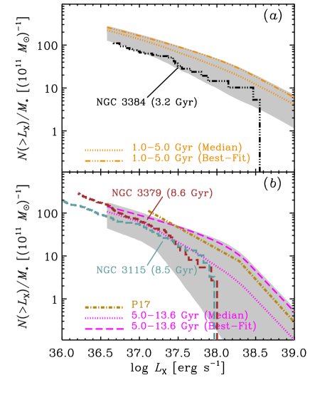
Figure 14.— ($a$) Expanded view of the 1–5 Gyr SFH XLF model. We show both the best-fit model (orange triple-dot-dashed curve), as well as the median model (orange dotted curve) with 1$\sigma$ error envelope (gray shaded region). For comparison, we show the XLF of field LMXBs in NGC 3384 (black triple-dot-dashed curve), an elliptical galaxy with mass-weighted stellar age of $\approx$3.2 Gyr. ($b$) Expanded view of the 5–13.6 Gyr SFH XLF model. Here the best-fit model (dashed magenta curve) lies outside of the 1$\sigma$ error envelope. The XLFs for field LMXBs in NGC 3379 and 3115, which have light-weighted stellar ages of 8.6 and 8.5 Gyr, respectively, have been shown for comparison (Lehmer et al. 2014). Also, the average field LMXB XLF for nine nearby ellipticals with 9–11.5 Gyr old populations is plotted as a dotted gold curve (Peacock & Zepf 2016; Peacock et al. 2017). The comparison field LMXB XLFs appear to show reasonable agreement with the model XLFs derived here from M51, but show some minor differences in the XLF shapes.

4. Discussion

In the previous section ($\S$3.4), we presented a comprehensive model for how the generalized XRB XLF evolves with age, as derived from M51 alone. We note that such a model, by definition, is meant to be applicable to describing how XRB populations form over time in galaxies generally (however, see discussion of caveats below). As such, we can make comparisons between our model estimates and a number of other observations and XRB population synthesis model predictions.

In Figure 14, we show expanded views of our XLF models for 1–5 Gyr and 5–13.6 Gyr ages, and now include the median model (dotted curves) and 1$\sigma$ error envelopes (i.e., the 16–84% confidence range). Note that the best-fit model for the 5–13.6 Gyr age range (i.e., Fig. 14$b$) mainly lies outside of the 1$\sigma$ range around the median. This is driven by the very long tail in the distribution of the $\alpha_{2}({\rm 10~{}Gyr})$ probablity distribution (see Fig. 11), which leads to large uncertainties in the XRB XLF at large ages. For direct comparison, we show the field LMXB XLFs for elliptical galaxies NGC 3384, NGC 3379, and NGC 3115 (based on Lehmer et al. 2014), which have light-weighted stellar ages of $\approx$3.2, 8.6, and 8.5 Gyr, respectively. We also show, in Figure 14$b$, the best-fit average field LMXB XLF from Peacock et al. (2017), which was derived using nine nearby elliptical galaxies with light-weighted stellar ages spanning $\approx$9–11.5 Gyr (Peacock & Zepf 2016). We note that at a very peripheral level, the XLFs of the local ellipticals with $\;\buildrel>\over{\sim}\;$8 Gyr populations played a role in our chosen fixed value of $\alpha_{3}({\rm 10~{}Gyr})$ (see $\S$3.4 for details), but otherwise played no role in the development of our SFH XLF model. Nonetheless, our best-fit models from M51 provide very reasonable descriptions of the XLFs for all three elliptical galaxies and the Peacock et al. (2017) average field LMXB XLF, but with large uncertainties.

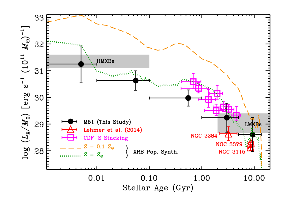
Figure 15.— Constraints on the X-ray power output evolution for XRB populations, normalized by a birth mass of $M_{0}=10^{11}$ $M_{\odot}$. The black filled circles represent the XRB X-ray luminosity evolution as derived from our best-fit SFH XLF model for M51 (see Fig. 10$a$ and Equation (13)). Estimates from HMXB and LMXB scaling relations (gray rectangles), field LMXBs in three elliptical galaxies (red triangles), and results from X-ray stacking analyses in the $\approx$6 Ms CDF-S (magenta squares) have been plotted for comparison (see $\S$4 for details). XRB population synthesis trajectories have been overlayed for XRB populations born with solar ($Z_{\odot}$; green dotted curve) and tenth solar (0.1 $Z_{\odot}$; orange dashed curve) metallicity. We find that our constraints from M51 suggest lower XRB X-ray power output at $\approx$0.6–5 Gyr compared to the CDF-S data; however, this offset may be related to the significantly higher metallicity in M51 ($\approx$2–3 $Z_{\odot}$) versus the CDF-S galaxies ($\approx$0.8–1.2 $Z_{\odot}$).

The direct comparison of our SFH XLF models with observed XLFs from field LMXBs in other elliptical galaxies of varying ages may not be completely appropriate. For instance, stellar ages of elliptical galaxies are inferred from optical spectra, taking advantage of absorption feature strengths and single stellar population synthesis modeling (see, e.g., McDermid et al. 2006; Sánchez-Blázquez et al. 2006; Thomas et al. 2010). As such, the ages are stellar-light weighted, when almost certainly some SFH needs to be accounted for. Also, the XRB population modeling in our work is statistical in nature and does not directly distinguish between LMXB populations in globular clusters (GCs) versus those found in the field. The elliptical galaxy comparison XLFs presented here have GC LMXB populations removed (see Lehmer et al. 2014 for details), since elliptical galaxies are generally much more rich in GC LMXBs than spiral galaxies like M51, which are dominated by field LMXBs. However, M51 may still have a significant GC LMXB population, which we have not accounted for here. Despite these issues, our simple age-dependent SFH XLF model of M51 provides a very similar resemblance to the elliptical galaxy field LMXB XLFs, albeit with large uncertainties.

By integrating Equation (10), we can obtain a direct prediction for how the X-ray power output of the cumulative XRB population evolves over time following a star formation event. Specifically, the X-ray power output per unit birth stellar mass, $M_{0}$, can be obtained following:

$$L_{\rm X}(t)/M_{0}=\left(\frac{M_{\star}(t)}{M_{0}}\right)\int_{L_{\rm lo}}^{L_{c}}L_{\rm X}h(L_{\rm X},t)dL_{\rm X},$$ (14)

where $L_{\rm lo}=0.01$ (i.e., 10³⁶ erg s^-1) is a lower integration limit, below which the XLF is observed to turn over and contribution from XRBs are negligible (see, e.g., studies of the XLF in the MW and Magellanic Clouds from Grimm et al. 2002). The term $M_{\star}(t)/M_{0}$ quantifies the present-day stellar mass to birth mass ratio as a function of age, and is determined by our stellar population synthesis modeling; $\log M_{\star}(t)/M_{0}=$ $-0.02$, $-0.10$, $-0.19$, $-0.27$, and $-0.33$ at 5 Myr, 55 Myr, 550 Myr, 3 Gyr, and 9 Gyr, respectively. In Figure 15, we show $\log L_{\rm X}(t)/M_{0}$ versus age, as derived for the M51 population. Our results suggest that the X-ray power output of XRB populations declines by $\approx$3–4 orders of magnitude from $\approx$10 Myr to $\approx$10 Gyr due to the combined decline in XLF normalization and steepening in slope with increasing age (see Fig. 12$a$).

We can compare the trend observed in Figure 15 with expectations estimated from X-ray scaling relations. For instance, at the young stellar-age end, we can use the $L_{\rm X}$(HMXB)/SFR relation to provide an order-of-magnitude estimate of $L_{\rm X}/M_{0}$ for the $\;\buildrel<\over{\sim}\;$100 Myr population. Typically, SFR values are estimated as the mean SFR over the last 100 Myr, due to the fact that SFR tracers provide emission on those time scales. If the X-ray emission is indeed associated with the $\;\buildrel<\over{\sim}\;$100 Myr old population, then we can make the following estimate:

$$\langle L_{\rm X}(\lower 2.15277pt\hbox{$\;\buildrel<\over{\sim}\;$}{\rm 100~{}Myr})/M_{0}\rangle\approx\left(\frac{L_{\rm X}{\rm(HMXB)}}{\rm SFR}\right)\left(\frac{1}{100\times 10^{6}~{}{\rm yr}}\right).$$

Recent scaling relation studies have estimated $\log L_{\rm X}$(HMXB)/SFR $=$ 39.1–39.6 (Lehmer et al. 2010, 2016; Mineo et al. 2012) or $\log\langle L_{\rm X}(\lower 2.15277pt\hbox{$\;\buildrel<\over{\sim}\;$}{\rm 100~{}Myr})/M_{0}\rangle\approx$ 31.1–31.6. For LMXBs, scaling relations based on both star-forming and elliptical galaxy populations indicate $\log L_{\rm X}{\rm(LMXB)}/M_{\star}$ = 29.0–29.6 (e.g., Lehmer et al. 2010, 2016; Boroson et al. 2011; Zhang et al. 2012). These galaxy samples span effective ages of $\approx$2–15 Gyr, so correcting to their birth stellar mass implies $\log L_{\rm X}{\rm(LMXB)}/M_{0}$ = 28.6–29.4 (i.e., $\log M_{\star}/M_{0}=$ $-0.33$ to $-0.2$). We note that the quoted scaling relations were derived without making any corrections for GC LMXBs, which will enhance the LMXB emission over M51 for the case of the ellipticals. In Figure 15, we indicate the estimated regions for HMXB and LMXB populations based on scaling relations as gray rectangles with annotations. We find good agreement, within the uncertainties, between the HMXB scaling relations and our M51-based predictions for HMXB emission, while the LMXB scaling relations predict $L_{\rm X}/M_{0}$ values that are somewhat higher than our estimates for M51 at $\approx$10 Gyr, albeit still within errors. Such a difference, however, could be due to the disproportionate boost to the scaling relations from the GC LMXB population (see below).

We can make further comparisons using additional observations that constrain the XRB X-ray emission at different ages. For example, in Figure 15, we show $L_{\rm X}/M_{0}$ values for the field LMXBs (red triangles) in NGC 3384, NGC 3379, and NGC 3115. As with the XLF models, the integrated $L_{\rm X}/M_{0}$ values are in good agreement with our M51-based prediction. This provides some indication that M51 has a weak contribution from GC LMXBs; however, direct counterpart studies are required to confirm this.

An additional constraint on $L_{\rm X}/M_{0}$ for various age ranges comes from the stacking analyses of distant galaxy populations from Lehmer et al. (2016), which are based on a $\approx$6 Ms exposure of the Chandra Deep Field-South (CDF-S; Luo et al. 2017) and provide measurements of how the $L_{\rm X}$(HMXB)/SFR and $L_{\rm X}$(LMXB)/$M_{\star}$ scaling relations evolved since $z\approx 2.3$. Here, we utilize the redshift-dependent $L_{\rm X}$(LMXB)/$M_{\star}$ scaling relation constraints from Lehmer et al. (2016), and estimate mass-weighted stellar ages for the redshift bins. These mass-weighted stellar ages were calculated by first extracting synthesized galaxy catalogs from the Millenium II cosmological simulation from Guo et al. (2011) that had the same SFR and $M_{\star}$ selection ranges as those adopted by Lehmer et al. (2016). These galaxy catalogs contain estimates of the mass-weighted stellar ages for each galaxy. The mass-weighted stellar age of the entire galaxy population (catalog) is then estimated using Equation (8), and a standard deviation of the population is calculated to estimate the error. All values are corrected by the single stellar population synthesis derived factor of $M_{\star}(t)/M_{0}$ to convert $L_{\rm X}$(LMXB)/$M_{\star}$ to $L_{\rm X}/M_{0}$.

The magenta squares in Figure 15 show the Lehmer et al. (2016) estimates of $L_{\rm X}/M_{0}$. The ages evaluated by the CDF-S stacking analyses span $\approx$600 Myr to $\approx$5 Gyr, corresponding to the $z\approx 2.3$ and $z\approx 0.4$ stacked populations, respectively. Over this age range, the $\approx$6 Ms CDF-S stacked constraints appear to be somewhat elevated above our M51-based estimates by a factor of $\approx$2. The derived scaling relations for galaxy samples in the CDF-S are expected to be appropriate for representative galaxies (in terms of representing the majority of the stellar mass) in the Universe, which are dominated by star-forming galaxies on the “main sequence” (e.g., Elbaz et al. 2007; Noeske et al. 2007; Karim et al. 2011; Whitaker et al. 2014). These galaxies will contain a broad range of stellar populations, and complex SFHs (like that of M51). Therefore taking the globally averaged X-ray luminosity per unit mass and associating it with a single mean stellar age for the population may not provide an entirely equivalent comparison to our M51 results, which have $L_{\rm X}/M_{0}$ values based on decomposition of all stellar age contributions. We can perform the equivalent operation for M51, however, by computing the galaxy-wide mean stellar age and extracting the LMXB emission per unit mass. Doing so, reveals $\langle t_{\rm age}\rangle\approx 5.2$ Gyr and $L_{\rm X}({\rm LMXB})/M_{0}\approx 29.1$ (based on the LMXB XLF derived in $\S$3.2), which is in nearly perfect agreement with the $L_{\rm X}/M_{0}$ estimates for the 1–5 Gyr age bin. It is therefore unlikely that the CDF-S estimates are systematically elevated from our M51 estimates simply due to differences in how the points were derived.

Alternatively, the apparent discrepancy between our results for M51 and those from the $\approx$6 Ms CDF-S stacking analyses may arise due to the high metallicity of M51 ($Z\approx$ 1.5–2.5 $Z_{\odot}$; e.g., Moustakas et al. 2010) relative to typical galaxies at $z\approx$ 0.3–2.3 ($Z\approx$ 0.8–1.2 $Z_{\odot}$; e.g., Madau & Fragos 2016). Population synthesis predictions have shown, and several studies now seem to confirm, that the XRB power output per stellar mass declines with increasing metallicity (e.g., Fragos et al. 2013; Basu-Zych et al. 2013a,b, 2016; Prestwich et al. 2013; Douna et al. 2015; Brorby et al. 2014, 2016; Lehmer et al. 2016). To clarify the expected level of this metallicity effect, we show in Figure 15 the Fragos et al. (2013) XRB population synthesis model predictions for the $Z_{\odot}$ and 0.1 $Z_{\odot}$ cases. We find that the CDF-S stacked data at $\approx$0.6–5 Gyr are in very good agreement with the $Z_{\odot}$ XRB population synthesis predictions. The 0.1 $Z_{\odot}$ XRB population synthesis model is almost uniformly an order of magnitude above the $Z_{\odot}$ case. Unfortunately, we do not have available XRB population synthesis models appropriate for 1.5–2.5 $Z_{\odot}$; however, if the nearly linear trend of declining $L_{\rm X}/M_{0}$ with metallicity were to continue, we might expect that most of the points in M51 would be factors of $\approx$2–3 times lower (i.e., $\approx$0.3–0.5 dex), and may explain the offset between the M51 and $\approx$6 Ms CDF-S data points at $\approx$0.6–5 Gyr.

5. Summary and Future Direction

We have presented a new technique for determining the XLF evolution of XRB populations in nearby galaxies that have resolved XRB populations (e.g., via Chandra observations) and multiwavelength data sufficient for determining accurate SFHs on subgalactic scales. We have performed SED fitting of far-UV–to–far-IR data to construct $M_{\star}$, SFR, and SFH maps, and we utilize the $\approx$850 ks cumulative Chandra exposure of M51 to constrain the XRB population demographics within the galaxy. We spatially segregate X-ray source populations within regions of varying sSFR and mean mass-weighted stellar age, and then self-consistently model how the XLFs vary accross these regions. Below, we summarize our key findings.

• By dividing the galaxy into regions with varying sSFR, we are able to decompose the XRB XLF into LMXB and HMXB contributions that scale with $M_{\star}$ and SFR, respectively ($\S$3.3). Our results are broadly consistent with past studies of the scaling of XRB XLFs from actively star-forming galaxy samples (e.g., Mineo et al. 2012) and passive ellipticals (e.g., Zhang et al. 2012). However, we find that our inferred LMXB XLF has an excess of $L_{\rm X}\geq 10^{38}$ erg s^-1 sources compared to elliptical galaxies (Fig. 8). This result is potentially due to the LMXB population in M51 being younger than typical ellipticals (i.e., $\approx$5 Gyr for M51 and $\approx$10 Gyr for ellipticals), as was hypothesized in Kuntz et al. (2016).

• When dividing the galaxy into regions based on the local mean stellar age, we were able to self-consistently model the XRB XLFs using an age-dependent model where the XLF shape and normalization evolve with time ($\S$3.4). Our best-fit model indicates that the normalization of the XRB XLF declines by $\sim$3–3.5 orders of magnitude from $\approx$10 Myr to $\approx$10 Gyr, while the overall XLF slope steepens over this time period (Fig. 12).

• Through a statistical comparison of models, we find that our generalized evolving XRB XLF model provides a better fit to the data in all subregions of M51 compared to the LMXB and HMXB decomposition model ($\S$3.4). In principle, this model is robust and applicable to XRB populations in other galaxies, provided the metallicities are similar and the XRBs are associated with the evolution of the underlying stellar populations. We find that our XRB XLF models for the $\approx$3–11.5 Gyr timescale provide good agreement with observed field LMXBs in elliptical galaxies of comparable ages, providing independent support for our model predictions ($\S$4 and Fig. 14).

• By integrating our evolving XRB XLF model with respect to $L_{\rm X}$, we can predict the total XRB X-ray power output evolution with age. These predictions are in good agreement with those provided by XRB population synthesis models, high-redshift stacking results, estimates from scaling relations, and field LMXBs in nearby elliptical galaxies (see $\S$4 and Fig. 15).

The above conclusions provide a step forward in empirically calibrating how XRB XLFs evolve with age, generally. However, we expect that the XRB evolutionary history will also be dependent on the metallicity history, since metallicity is expected to be a major factor in the formation of XRBs relative to the stellar population (see Fig. 15 and discussion in $\S$4). In the near future, we will apply the techniques developed here to a larger suite of $\sim$20 nearly face-on spiral galaxies, for which SFHs can be calculated well. With this larger sample, we will further expand our analyses to include XRB XLF evolution for samples separated into metallicity bins. Our ultimate goal will be to develop a full suite of age and metallicity dependent XRB XLF models that self-consistently describe well observed XRB XLFs in all nearby galaxies, but also X-ray scaling relations and their redshift evolution.

References

- Aird et al. (2017) Aird, J., Coil, A. L., & Georgakakis, A. 2017, MNRAS, 465, 3390
- Antoniou & Zezas (2016) Antoniou, V., & Zezas, A. 2016, MNRAS, 459, 528
- Basu-Zych et al. (2013) Basu-Zych, A. R., Lehmer, B. D., Hornschemeier, A. E., et al. 2013a, ApJ, 774, 152
- Basu-Zych et al. (2013) Basu-Zych, A. R., Lehmer, B. D., Hornschemeier, A. E., et al. 2013b, ApJ, 762, 45
- Basu-Zych et al. (2016) Basu-Zych, A. R., Lehmer, B., Fragos, T., et al. 2016, ApJ, 818, 140
- Belczynski et al. (2004) Belczynski, K., Kalogera, V., Zezas, A., & Fabbiano, G. 2004, ApJL, 601, L147
- Benacquista & Downing (2013) Benacquista, M. J., & Downing, J. M. B. 2013, Living Reviews in Relativity, 16, 4
- Boroson et al. (2011) Boroson, B., Kim, D.-W., & Fabbiano, G. 2011, ApJ, 729, 12
- Brandt & Podsiadlowski (1995) Brandt, N., & Podsiadlowski, P. 1995, MNRAS, 274, 461
- Broos et al. (2010) Broos, P. S., Townsley, L. K., Feigelson, E. D., Getman, K. V., Bauer, F. E., & Garmire, G. P. 2010, ApJ, 714, 1
- Brorby et al. (2014) Brorby, M., Kaaret, P., & Prestwich, A. 2014, MNRAS, 441, 2346
- Brorby et al. (2016) Brorby, M., Kaaret, P., Prestwich, A., & Mirabel, I. F. 2016, MNRAS, 457, 4081
- Cash (1979) Cash, W. 1979, ApJ, 228, 939
- Coulter et al. (2016) Coulter, D. A., Lehmer, B. D., Eufrasio, R. T., et al. 2016, arXiv:1612.05189
- Douna et al. (2015) Douna, V. M., Pellizza, L. J., Mirabel, I. F., & Pedrosa, S. E. 2015, A&A, 579, A44
- Elbaz et al. (2007) Elbaz, D., Daddi, E., Le Borgne, D., et al. 2007, A&A, 468, 33
- Fabbiano et al. (1982) Fabbiano, G., Feigelson, E., & Zamorani, G. 1982, ApJ, 256, 397
- Fabbiano (2006) Fabbiano, G. 2006, ARA&A, 44, 323
- Fioc & Rocca-Volmerange (1997) Fioc, M., & Rocca-Volmerange, B. 1997, A&A, 326, 950
- Fragos et al. (2008) Fragos, T., Kalogera, V., Belczynski, K., et al. 2008, ApJ, 683, 346
- Fragos et al. (2013) Fragos, T., Lehmer, B., Tremmel, M., et al. 2013a, ApJ, 764, 41
- Fragos et al. (2013) Fragos, T., Lehmer, B. D., Naoz, S., Zezas, A., & Basu-Zych, A. 2013b, ApJL, 776, L31
- Freeman et al. (2002) Freeman, P. E., Kashyap, V., Rosner, R., & Lamb, D. Q. 2002, ApJS, 138, 185
- Georgakakis et al. (2008) Georgakakis, A., Nandra, K., Laird, E. S., Aird, J., & Trichas, M. 2008, MNRAS, 388, 1205
- Gilfanov (2004) Gilfanov, M. 2004, MNRAS, 349, 146
- Gilfanov et al. (2004) Gilfanov, M., Grimm, H.-J., & Sunyaev, R. 2004, MNRAS, 351, 1365
- Grimm et al. (2002) Grimm, H.-J., Gilfanov, M., & Sunyaev, R. 2002, A&A, 391, 923
- Guo et al. (2011) Guo, Q., White, S., Boylan-Kolchin, M., De Lucia, G., Kauffmann, G., Lemson, G., Li, C., Springel, V., & Weinmann, S. 2011, MNRAS, 413, 101
- Hornschemeier et al. (2001) Hornschemeier, A. E., Brandt, W. N., Garmire, G. P., et al. 2001, ApJ, 554, 742
- Jarrett et al. (2003) Jarrett, T. H., Chester, T., Cutri, R., Schneider, S. E., & Huchra, J. P. 2003, AJ, 125, 525
- Kaaret et al. (2011) Kaaret, P., Schmitt, J., & Gorski, M. 2011, ApJ, 741, 10
- Karim et al. (2011) Karim, A., Schinnerer, E., Martínez-Sansigre, A., et al. 2011, ApJ, 730, 61
- Kennicutt (1998) Kennicutt, R. C., Jr. 1998, ARA&A, 36, 189
- Kennicutt & Evans (2012) Kennicutt, R. C., & Evans, N. J. 2012, ARA&A, 50, 531
- Kilgard et al. (2002) Kilgard, R. E., Kaaret, P., Krauss, M. I., et al. 2002, ApJ, 573, 138
- Kilgard et al. (2005) Kilgard, R. E., Cowan, J. J., Garcia, M. R., et al. 2005, ApJS, 159, 214
- Kim et al. (2007) Kim, M., Kim, D.-W., Wilkes, B. J., et al. 2007, ApJS, 169, 401
- Kim et al. (2009) Kim, D.-W., Fabbiano, G., Brassington, N. J., et al. 2009, ApJ, 703, 829
- Kim & Fabbiano (2010) Kim, D.-W., & Fabbiano, G. 2010, ApJ, 721, 1523
- Kong et al. (2003) Kong, A. K. H., DiStefano, R., Garcia, M. R., & Greiner, J. 2003, ApJ, 585, 298
- Kroupa (2001) Kroupa, P. 2001, MNRAS, 322, 231
- Kundu et al. (2007) Kundu, A., Maccarone, T. J., & Zepf, S. E. 2007, ApJ, 662, 525
- Kuntz et al. (2016) Kuntz, K. D., Long, K. S., & Kilgard, R. E. 2016, ApJ, 827, 46
- Lehmer et al. (2007) Lehmer, B. D., Brandt, W. N., Alexander, D. M., et al. 2007, ApJ, 657, 681
- Lehmer et al. (2010) Lehmer, B. D., Alexander, D. M., Bauer, F. E., Brandt, W. N., Goulding, A. D., Jenkins, L. P., Ptak, A., & Roberts, T. P. 2010, ApJ, 724, 559
- Lehmer et al. (2014) Lehmer, B. D., Berkeley, M., Zezas, A., et al. 2014, ApJ, 789, 52
- Lehmer et al. (2015) Lehmer, B. D., Tyler, J. B., Hornschemeier, A. E., et al. 2015, ApJ, 806, 126
- Lehmer et al. (2016) Lehmer, B. D., Basu-Zych, A. R., Mineo, S., et al. 2016, ApJ, 825, 7
- Lin et al. (2015) Lin, D., Irwin, J. A., Wong, K.-W., et al. 2015, ApJ, 808, 20
- Luo et al. (2017) Luo, B., Brandt, W. N., Xue, Y. Q., et al. 2017, ApJS, 228, 2
- Maccarone et al. (2014) Maccarone, T. J., Girard, T. M., & Casetti-Dinescu, D. I. 2014, MNRAS, 440, 1626
- Madau & Dickinson (2014) Madau, P., & Dickinson, M. 2014, ARA&A, 52, 415
- McDermid et al. (2006) McDermid, R. M., Emsellem, E., Shapiro, K. L., et al. 2006, MNRAS, 373, 906
- McQuinn et al. (2016) McQuinn, K. B. W., Skillman, E. D., Dolphin, A. E., Berg, D., & Kennicutt, R. 2016, ApJ, 826, 21
- Mineo et al. (2012) Mineo, S., Gilfanov, M., & Sunyaev, R. 2012a, MNRAS, 419, 2095
- Mineo et al. (2012) Mineo, S., Gilfanov, M., & Sunyaev, R. 2012b, MNRAS, 426, 1870
- Mineo et al. (2014) Mineo, S., Fabbiano, G., D’Abrusco, R., et al. 2014, ApJ, 780, 132
- Moustakas et al. (2010) Moustakas, J., Kennicutt, R. C., Jr., Tremonti, C. A., et al. 2010, ApJS, 190, 233-266
- Noeske et al. (2007) Noeske, K. G., Weiner, B. J., Faber, S. M., et al. 2007, ApJL, 660, L43
- Peacock et al. (2014) Peacock, M. B., Zepf, S. E., Maccarone, T. J., et al. 2014, ApJ, 784, 162
- Peacock & Zepf (2016) Peacock, M. B., & Zepf, S. E. 2016, ApJ, 818, 33
- Peacock et al. (2017) Peacock, M. B., Zepf, S. E., Kundu, A., et al. 2017, ApJ, 841, 28
- Pereira-Santaella et al. (2011) Pereira-Santaella, M., Alonso-Herrero, A., Santos-Lleo, M., et al. 2011, A&A, 535, A93
- Podsiadlowski et al. (2005) Podsiadlowski, P., Pfahl, E., & Rappaport, S. 2005, Binary Radio Pulsars, 328, 327
- Prestwich et al. (2013) Prestwich, A. H., Tsantaki, M., Zezas, A., et al. 2013, ApJ, 769, 92
- Repetto et al. (2012) Repetto, S., Davies, M. B., & Sigurdsson, S. 2012, MNRAS, 425, 2799
- Repetto et al. (2017) Repetto, S., Igoshev, A. P., & Nelemans, G. 2017, MNRAS,
- Sánchez-Blázquez et al. (2006) Sánchez-Blázquez, P., et al. 2006, A&A, 457, 809
- Stark et al. (1992) Stark, A. A., Gammie, C. F., Wilson, R. W., Bally, J., Linke, R. A., Heiles, C., & Hurwitz, M. 1992, ApJS, 79, 77
- Sarazin et al. (2000) Sarazin, C. L., Irwin, J. A., & Bregman, J. N. 2000, ApJL, 544, L101
- Soria & Wu (2003) Soria, R., & Wu, K. 2003, A&A, 410, 53
- Thomas et al. (2010) Thomas, D., Maraston, C., Schawinski, K., Sarzi, M., & Silk, J. 2010, MNRAS, 404, 1775
- Trudolyubov et al. (2002) Trudolyubov, S. P., Borozdin, K. N., Priedhorsky, W. C., Mason, K. O., & Cordova, F. A. 2002, ApJL, 571, L17
- Tzanavaris et al. (2013) Tzanavaris, P., Fragos, T., Tremmel, M., et al. 2013, ApJ, 774, 136
- Voss & Gilfanov (2006) Voss, R., & Gilfanov, M. 2006, A&A, 447, 71
- Voss et al. (2009) Voss, R., Gilfanov, M., Sivakoff, G. R., et al. 2009, ApJ, 701, 471
- Whitaker et al. (2014) Whitaker, K. E., Franx, M., Leja, J., et al. 2014, ApJ, 795, 104
- Zezas et al. (2006) Zezas, A., Fabbiano, G., Baldi, A., et al. 2006, ApJS, 166, 211
- Zhang et al. (2012) Zhang, Z., Gilfanov, M., & Bogdán, Á. 2012, A&A, 546, A36
- Zhang et al. (2013) Zhang, Z., Gilfanov, M., & Bogdán, Á. 2013, A&A, 556, A9